Casimir-Polder energy landscape: Unipolarizable atom and ring

Abstract

The Casimir-Polder interaction energy between a unipolarizable point atom and a unipolarizable dielectric ring has been limited, until now, to the case when the atom is confined on the axis of symmetry of the ring. We find the generalized analytical expression for any position of the atom relative to the ring in terms of complete elliptic integrals. This is aided by the construction of a class of integrals of a Jacobian elliptic function as a linear combination of complete elliptic integrals. Our expression for the interaction energy allows us to investigate the instability of the atom even for the equilibrium points which exists off the axis of symmetry.

1 Introduction

The Casimir-Polder interaction is the long-range retarded effect associated with the Casimir effect [7], where it is typically dominated by the zero-frequency (static) mode. The retardation leads to the inverse seventh power law behavior, in contrast to the inverse sixth power law decay of the non-retarded London and van der Waals interaction energy [28, 12, 17, 14], becoming one of the earliest demonstration of an interplay between quantum and relativistic effects in a system. It was also realized early on that these interactions could exhibit repulsive forces between polarizable atoms [3, 22, 9, 8, 4]. More recently, in Ref. [16], it was shown that the interaction energy between an elongated needle-shaped-conductor and a perfectly conducting metal sheet with a circular aperture could also exhibit repulsion. This led to investigations of similar configurations in the non-retarded van der Waals regime in Refs. [11] and [1] and an analytic expression for the retarded Casimir-Polder interaction energy between a unipolarizable atom and a dielectric plate with a circular aperture was derived in Refs. [20] and [25]. Later, in Refs. [19, 18] a closed-form expression for the retarded energy for the case of circular dielectric ring and an atom was derived. A limitation of all of the above investigations is that the position of the atom is restricted to the axis of symmetry of the configuration. Even though this restriction simplifies the problem sufficiently for the interaction energy to have a simple form in terms of rational functions, it doesn’t allow for any stability analysis.

Our results generalize the interaction energy when the atom is off the axis of symmetry of the ring. We show that the Casimir-Polder interaction energies between a unipolarizable atom and a unipolarizable dielectric ring admits exact solutions in terms of elliptic integrals. In particular, we accomplish this for one of the many configurations considered in Ref. [18, 19] when the atom is no more restricted to the axis of symmetry. Even though it was realized early on that in this configuration the unipolarizable atom has radial instability everywhere on the symmetry axis, the analytical expression for the interaction energy we present here allows us to explore the nature of instability concretely in the vicinity of equilibrium points even when these points are off the axis of symmetry.

In the next section (Section 2), we describe our system constituting of a unipolarizable atom and a unipolarizable dielectric ring. We introduce the expression for the Casimir-Polder interaction energy for the configuration as an integral over an azimuth angle. In Section 3, we review and collect the relevant results in Ref. [19] when the unipolarizable atom is confined on the axis of symmetry. In Section 4, we construct a class of integrals of a Jacobian elliptic function $\pi_{n}(k)$ and express them as a linear combination of complete elliptic integrals. A recurrence relation for $\pi_{n}(k)$ is presented [30]. In terms of these elliptic integrals, in Section 5, we derive a generalized expression for the Casimir-Polder interaction energy between a unipolarizable atom and a unipolarizable dielectric ring when the atom is off the axis of the symmetry of the configuration. We reproduce the interaction energy in Ref. [19] when the atom is confined to the axis of symmetry. In Section 6, we investigate the nature of stability of the atom when it is placed on the equilibrium points for a couple of orientations of the polarizability of atom. We present an outlook and conclusion in Section 7.

2 Casimir-Polder energy

The Casimir-Polder interaction energy between a unipolarizable point atom described by its atomic polarizability ${\bm{\alpha}}$ and a unipolarizable dielectric of susceptibility tensor ${\bm{\chi}}$ is given by [18]

$$E({\bm{\alpha}},{\bm{\chi}};{\bf r})=-\frac{\hbar c}{32\pi^{2}}\int\frac{d^{3}r^{\prime}}{|{\bf r}^{\prime}-{\bf r}|^{7}}\Big[13\,\text{tr}({\bm{\alpha}}\cdot{\bm{\chi}})\hskip 42.67912pt$$

$$\hskip 28.45274pt-56(\hat{\bf s}\cdot{\bm{\alpha}}\cdot{\bm{\chi}}\cdot\hat{\bf s})+63(\hat{\bf s}\cdot{\bm{\alpha}}\cdot\hat{\bf s})(\hat{\bf s}\cdot{\bm{\chi}}\cdot\hat{\bf s})\Big],$$ (2.1)

where the unit vector

$$\hat{\bf s}=\frac{{\bf r}^{\prime}-{\bf r}}{|{\bf r}^{\prime}-{\bf r}|}$$ (2.2)

is constructed out of vector

$${\bf s}={\bf r}^{\prime}-{\bf r},$$ (2.3)

which describes the relative position ${\bf r}$ of the atom with respect to a point ${\bf r}^{\prime}$ on the dielectric. Here $\hbar$ is the rationalized Planck constant and $c$ is speed of light in vacuum. For the case of dielectrics with uniform susceptibility the Casimir-Polder interaction energy,

$$E({\bm{\alpha}},{\bm{\chi}};{\bf r}) = -\frac{\hbar c}{32\pi^{2}}\,\text{tr}\Big[13\,({\bm{\alpha}}\cdot{\bm{\chi}})M_{0}-56({\bm{\alpha}}\cdot{\bf M}_{2}\cdot{\bm{\chi}})$$ (2.4)

$$\hskip 45.5244pt+63({\bm{\alpha}}\cdot{\bf M}_{4}\cdot{\bm{\chi}})\Big],$$

can be expressed in terms of a zero-rank tensor, a scalar,

$$M_{0}=\int d^{3}r^{\prime}\,\frac{1}{s^{7}},$$ (2.5)

a second-rank tensor

$${\bf M}_{2}=\int d^{3}r^{\prime}\,\frac{\hat{\bf s}\,\hat{\bf s}}{s^{7}},$$ (2.6)

and a fourth-rank tensor

$${\bf M}_{4}=\int d^{3}r^{\prime}\,\frac{\hat{\bf s}\,\hat{\bf s}\,\hat{\bf s}\,\hat{\bf s}}{s^{7}}.$$ (2.7)

The ‘dot’ operations in $({\bm{\alpha}}\cdot{\bf M}_{4}\cdot{\bm{\chi}})$ comprises of trace operations between second rank tensors (that are suitably represented as dyadics) and a fourth rank tensor,

$$(\hat{\bf s}\cdot{\bm{\alpha}}\cdot\hat{\bf s})(\hat{\bf s}\cdot{\bm{\chi}}\cdot\hat{\bf s}) = \text{tr}\,\big[({\bm{\alpha}}\cdot\hat{\bf s})\,\hat{\bf s}\big]\;\text{tr}\,\big[\hat{\bf s}\,(\hat{\bf s}\cdot{\bm{\chi}})\big]$$ (2.8)

$$= \text{tr}\,({\bm{\alpha}}\cdot{\bf M}_{4}\cdot{\bm{\chi}}),$$

and is merely for typographic brevity.

Figure 1: A unipolarizable point atom with polarizability $\bm{\alpha}=\alpha_{1}\hat{\textbf{n}}\hat{\textbf{n}}$ at position ${\bf r}$ above a dielectric ring of radius $a$ with uniform polarizability $\bm{\sigma}=\sigma_{2}\hat{\textbf{z}}\hat{\textbf{z}}$. The point atom is a distance $\rho$ away from the axis of the ring. The principal axis $\hat{\bf n}$ of the atomic polarizability $\bm{\alpha}$ subtends an angle $\theta_{1}$ with respect to polarizability of the ring and the axis of the symmetry, that is, $\hat{\textbf{n}}\cdot\hat{\textbf{z}}=\cos\theta_{1}$

.

(a) Atom and ring

In this article, for simplicity, we shall confine our attention to the case of a polarizable atom that is polarizable only in a particular direction, say $\hat{\bf n}$, such that, it’s atomic polarizability can be expressed in the form

$${\bm{\alpha}}=\alpha_{1}\hat{\bf n}\hat{\bf n},$$ (2.9)

where $\alpha_{1}$ describes the magnitude of the atomic polarizability of the atom and $\hat{\bf n}$ is the direction of polarizability. We will call such an atom a completely anisotropically polarizable atom, or simply a unipolarizable atom. Similarly, for simplicity, we shall choose the direction of polarization of the dielectric ring to be the $\hat{\bf z}$ axis and the magnitude of polarization to be $\sigma_{2}$. Thus, the ring is described by the susceptibility,

$${\bm{\chi}}=\sigma_{2}\,\hat{\bf z}\hat{\bf z}\,\delta(z^{\prime}-0)\delta(\rho^{\prime}-a),$$ (2.10)

where $a$ is the radius of the ring and coordinates $z^{\prime}$, $\rho^{\prime}$, and $\phi^{\prime}$, represent the vector ${\bf r}^{\prime}$ that are integrated over in the expression for energy in Eq. (2.1). Then, the volume element $d^{3}r^{\prime}$ in the expression for energy is $d^{3}r^{\prime}=ad\rho^{\prime}d\phi^{\prime}dz^{\prime}$ and after completing the integrations in $z^{\prime}$ and $\rho^{\prime}$, we can express the interaction energy between the atom and ring in the form

$$E({\bm{\alpha}},{\bm{\chi}};{\bf r})=-\frac{\hbar c\alpha_{1}\sigma_{2}}{32\pi^{2}}\int_{0}^{2\pi}\frac{ad\phi^{\prime}}{s^{7}}\Big[13\,(\hat{\bf n}\cdot\hat{\bf z})^{2}\hskip 42.67912pt$$

$$-56(\hat{\bf s}\cdot\hat{\bf n})(\hat{\bf n}\cdot\hat{\bf z})(\hat{\bf z}\cdot\hat{\bf s})+63(\hat{\bf n}\cdot\hat{\bf s})^{2}(\hat{\bf z}\cdot\hat{\bf s})^{2}\Big],\hskip 22.76219pt$$ (2.11)

where ${\bf s}$ defined in Eq. (2.3), in the configuration under consideration in FIG. 1 are given in terms of

$${\bf r} = \rho\,\hat{\bm{\rho}}+z\hat{\bf z},$$ (2.12a)

$${\bf r}^{\prime} = a\,\hat{\bm{\rho}}^{\prime},$$ (2.12b)

with

$$\hat{\bm{\rho}} = \cos\phi\,\hat{\bf x}+\sin\phi\,\hat{\bf y},$$ (2.13a)

$$\hat{\bm{\rho}}^{\prime} = \cos\phi^{\prime}\hat{\bf x}+\sin\phi^{\prime}\hat{\bf y}.$$ (2.13b)

Using the completeness relation,

$${\bf 1}=\hat{\bm{\rho}}\hat{\bm{\rho}}+\hat{\bm{\phi}}\hat{\bm{\phi}}+\hat{\bf z}\hat{\bf z},$$ (2.14)

we can write

$$\hat{\bm{\rho}}^{\prime} = \hat{\bm{\rho}}^{\prime}\cdot(\hat{\bm{\rho}}\hat{\bm{\rho}}+\hat{\bm{\phi}}\hat{\bm{\phi}}+\hat{\bf z}\hat{\bf z})$$ (2.15a)

$$= (\hat{\bm{\rho}}^{\prime}\cdot\hat{\bm{\rho}})\hat{\bm{\rho}}+(\hat{\bm{\rho}}^{\prime}\cdot\hat{\bm{\phi}})\hat{\bm{\phi}}+(\hat{\bm{\rho}}^{\prime}\cdot\hat{\bf z})\hat{\bf z}$$ (2.15b)

$$= \cos(\phi^{\prime}-\phi)\hat{\bm{\rho}}+\sin(\phi^{\prime}-\phi)\hat{\bm{\phi}}.$$ (2.15c)

Thus, we can show that the relative position vector ${\bf s}$ in Eq. (2.3) can be written in the form

$${\bf s}=[a\cos(\phi^{\prime}-\phi)-\rho]\,\hat{\bm{\rho}}+a\sin(\phi^{\prime}-\phi)\,\hat{\bm{\phi}}-z\,\hat{\bf z}$$ (2.16)

with magnitude

$$s=\sqrt{a^{2}+z^{2}+\rho^{2}-2a\rho\cos(\phi^{\prime}-\phi)}.$$ (2.17)

Substituting $\phi^{\prime}-\phi\to\phi^{\prime}$, and using the fact that the integral in Eq. (2.11) is fundamentally a sum that is independent of the order of addition, we have

$$E({\bm{\alpha}},{\bm{\chi}};{\bf r})=-\frac{\hbar c\alpha_{1}\sigma_{2}}{32\pi^{2}}\int_{-\pi}^{\pi}\frac{ad\phi^{\prime}}{s^{7}}\Big[13\,(\hat{\bf n}\cdot\hat{\bf z})^{2}\hskip 42.67912pt$$

$$-56(\hat{\bf s}\cdot\hat{\bf n})(\hat{\bf n}\cdot\hat{\bf z})(\hat{\bf z}\cdot\hat{\bf s})+63(\hat{\bf n}\cdot\hat{\bf s})^{2}(\hat{\bf z}\cdot\hat{\bf s})^{2}\Big],\hskip 22.76219pt$$ (2.18)

where we suppressed the dependence on $\phi^{\prime}$ in $\hat{\bf s}(\phi^{\prime})$ and $s(\phi^{\prime})$, that is,

$${\bf s}(\phi^{\prime})=(a\cos\phi^{\prime}-\rho)\,\hat{\bm{\rho}}+a\sin\phi^{\prime}\,\hat{\bm{\phi}}-z\,\hat{\bf z}.$$ (2.19)

We gain some additional insight for the form of the interaction by expressing the energy in the form

$$E({\bm{\alpha}},{\bm{\chi}};{\bf r})=-\frac{\hbar c}{32\pi^{2}}\frac{\alpha_{1}\sigma_{2}}{a^{6}}\Big[13\,(\hat{\bf z}\cdot\hat{\bf n})^{2}M_{0}\hskip 56.9055pt$$

$$-56(\hat{\bf z}\cdot\hat{\bf n})(\hat{\bf n}\cdot{\bf M}_{2}\cdot\hat{\bf z})+63\,\hat{\bf n}\cdot(\hat{\bf n}\cdot{\bf M}_{4}\cdot\hat{\bf z})\cdot\hat{\bf z}\Big],\hskip 19.91692pt$$ (2.20)

where the tensors, now specific to the configuration of atom and ring in FIG. 1,

$$M_{0}=\int_{-\pi}^{\pi}d\phi^{\prime}\,\frac{a^{7}}{s^{7}}$$ (2.21)

is a scalar,

$${\bf M}_{2}=a^{7}\int_{-\pi}^{\pi}d\phi^{\prime}\,\frac{\hat{\bf s}\,\hat{\bf s}}{s^{7}},$$ (2.22)

is a second-rank tensor written as a dyadic, and

$${\bf M}_{4}=a^{7}\int_{-\pi}^{\pi}d\phi^{\prime}\,\frac{\hat{\bf s}\,\hat{\bf s}\,\hat{\bf s}\,\hat{\bf s}}{s^{7}}.$$ (2.23)

is a completely symmetric fourth-rank tensor. The order of vector operations in the construction

$$\hat{\bf n}\cdot(\hat{\bf n}\cdot{\bf M}_{4}\cdot\hat{\bf z})\cdot\hat{\bf z}$$ (2.24)

is unambiguous because of the complete symmetry in the tensor ${\bf M}_{4}$. That is, the dot products contract the adjacent vectors.

Significant simplification is achieved because we confined the polarization of the dielectric ring to be in the $\hat{\bf z}$ direction. This leads to

$$\hat{\bf n}\cdot{\bf M}_{2}\cdot\hat{\bf z}=-za^{7}\int_{-\pi}^{\pi}d\phi^{\prime}\frac{[\hat{\bf n}\cdot{\bf s}(\phi^{\prime})]}{s^{9}}$$ (2.25)

using $\hat{\bf z}\cdot{\bf s}(\phi^{\prime})=-z$ and

$$\hat{\bf n}\cdot(\hat{\bf n}\cdot{\bf M}_{4}\cdot\hat{\bf z})\cdot\hat{\bf z}=z^{2}a^{7}\int_{-\pi}^{\pi}d\phi^{\prime}\frac{[\hat{\bf n}\cdot{\bf s}(\phi^{\prime})]^{2}}{s^{11}}$$ (2.26)

in terms of ${\bf s}(\phi^{\prime})$ that was introduced in Eq. (2.19). The scalar construction appearing in the above expression is

$$\hat{\bf n}\cdot{\bf s}(\phi^{\prime})=(a\cos\phi^{\prime}-\rho)(\hat{\bf n}\cdot\hat{\bm{\rho}})+a\sin\phi^{\prime}(\hat{\bf n}\cdot\hat{\bm{\phi}})-z\,(\hat{\bf n}\cdot\hat{\bf z}),$$ (2.27)

where all the $\phi^{\prime}$ dependence has been presented explicitly. In particular, note that the constructions $(\hat{\bf n}\cdot\hat{\bm{\rho}})$, $(\hat{\bf n}\cdot\hat{\bm{\phi}})$, and $(\hat{\bf n}\cdot\hat{\bf z})$, do not have $\phi^{\prime}$ dependence in them.

3 Atom on the axis of symmetry

When the polarizable atom is positioned on the axis of symmetry of the ring, without its direction of polarizability $\hat{\bf n}$ necessarily along the axis, we have

$$\rho=0$$ (3.1)

and this leads to significant simplification in the expression for the magnitude in Eq. (2.17),

$$s\xrightarrow{\rho\to 0}\sqrt{a^{2}+z^{2}},$$ (3.2)

and in the expression for the vector in Eq. (2.16),

$${\bf s}(\phi^{\prime})\xrightarrow{\rho\to 0}a\cos\phi^{\prime}\hat{\bm{\rho}}+a\sin\phi^{\prime}\hat{\bm{\phi}}-z\,\hat{\bf z}.$$ (3.3)

As a consequence of the above simplifications we have the following exact evaluation of $M_{0}$ in Eq. (2.21)

$$M_{0}\xrightarrow{\rho\to 0} \;\frac{a^{7}}{(a^{2}+z^{2})^{\frac{7}{2}}}\int_{-\pi}^{\pi}d\phi^{\prime}$$

$$= \;2\pi\frac{a^{7}}{(a^{2}+z^{2})^{\frac{7}{2}}},$$ (3.4)

and the integral in Eq. (2.22) reduces to

$$\hat{\bf n}\cdot{\bf M}_{2}\cdot\hat{\bf z}\xrightarrow{\rho\to 0} \;-\frac{za^{7}}{(a^{2}+z^{2})^{\frac{9}{2}}}\int_{-\pi}^{\pi}d\phi^{\prime}[\hat{\bf n}\cdot{\bf s}(\phi^{\prime})]$$

$$= \;2\pi\frac{z^{2}a^{7}(\hat{\bf n}\cdot\hat{\bf z})}{(a^{2}+z^{2})^{\frac{9}{2}}},$$ (3.5)

and the integral in Eq. (2.23) leads to

$$\hat{\bf n}\cdot(\hat{\bf n}\cdot{\bf M}_{4}\cdot\hat{\bf z})\cdot\hat{\bf z}\xrightarrow{\rho\to 0}\frac{z^{2}a^{7}}{(a^{2}+z^{2})^{\frac{11}{2}}}\int_{-\pi}^{\pi}d\phi^{\prime}[\hat{\bf n}\cdot{\bf s}(\phi^{\prime})]^{2}$$

$$=2\pi\frac{z^{2}a^{7}}{(a^{2}+z^{2})^{\frac{11}{2}}}\frac{1}{2}\left[a^{2}+(2z^{2}-a^{2})(\hat{\bf n}\cdot\hat{\bf z})^{2}\right].\hskip 17.07164pt$$ (3.6)

Using the above the interaction energy in Eq. (2.20) takes the form, for ${\bf r}=z\,\hat{\bf z}$ when the atom is on the axis,

$$E({\bm{\alpha}},{\bm{\chi}};{\bf r})\xrightarrow{\rho\to 0}-\frac{\hbar c}{32\pi}\frac{\alpha_{1}\sigma_{2}a}{(a^{2}+z^{2})^{\frac{11}{2}}}\Big[63a^{2}z^{2}\hskip 42.67912pt$$

$$+(\hat{\bf n}\cdot\hat{\bf z})^{2}(26a^{4}-123a^{2}z^{2}+40z^{4})\Big].\hskip 11.38109pt$$ (3.7)

Using the realization of $\hat{\bf n}$ in terms of spherical polar coordinates, see FIG. 1,

$$\hat{\bf n}=\sin\theta_{1}\cos\phi_{1}\hat{\bf x}+\sin\theta_{1}\sin\phi_{1}\hat{\bf y}+\cos\theta_{1}\hat{\bf z},$$ (3.8)

such that

$$(\hat{\bf n}\cdot\hat{\bf z})^{2}=\cos^{2}\theta_{1}=\frac{1+\cos 2\theta_{1}}{2},$$ (3.9)

we can rewrite the interaction energy in Eq. (3.7) in the form

$$E({\bm{\alpha}},{\bm{\chi}};{\bf r})\xrightarrow{\rho\to 0}-\frac{\hbar c}{64\pi}\frac{\alpha_{1}\sigma_{2}a}{(a^{2}+z^{2})^{\frac{11}{2}}}\Big[(26a^{4}+3a^{2}z^{2}+40z^{4})$$

$$+\cos 2\theta_{1}(26a^{4}-123a^{2}z^{2}+40z^{4})\Big],\hskip 28.45274pt$$ (3.10)

which reproduces the result in Ref. [18].

When the atom is exactly at the center of the ring we have,

$$E({\bm{\alpha}},{\bm{\chi}};{\bf r})\xrightarrow[z\to 0]{\rho\to 0}-\frac{13\hbar c}{16\pi}\frac{\alpha_{1}\sigma_{2}}{a^{6}}(\hat{\bf n}\cdot\hat{\bf z})^{2},$$ (3.11)

which is 0 for $\hat{\bf n}\perp\hat{\bf z}$. The observation that energy is zero both when the atom is at the center of the ring and when the atom is at an infinite distance away on the axis of the ring, leads to the argument that the energy must have a minimum value. This non-trivial minimum for the energy is absent for $\hat{\bf n}\parallel\hat{\bf z}$. For the plate this argument led the authors in Ref. [16] to successfully find such a minimum in their configuration.

4 Complete elliptic integrals

The expression for Casimir-Polder energy when the atom is off the axis of symmetry of the ring, that will be derived in Section 5, is aided by the construction of a new set of elliptic integrals. These are known integrals of a Jacobian elliptic function, see 315.00 in Ref. [6], that are not widely encountered in literature. In this section, we define these elliptic integrals, $\pi_{n}(k)$ and introduce the relevant relations and identities for these integrals that are useful for our work.

Complete elliptic integrals of the first and second kind are defined by the integral representations [10]

$$K(k) = \int_{0}^{\frac{\pi}{2}}\frac{d\psi}{\sqrt{1-k^{2}\sin^{2}\psi}},$$ (4.1a)

$$E(k) = \int_{0}^{\frac{\pi}{2}}d\psi\sqrt{1-k^{2}\sin^{2}\psi},$$ (4.1b)

respectively, which are written here in Legendre’s notation [13, 6]. The elliptic modulus or eccentricity $k$ will be restricted to the domain $0\leq k<1$ in this discussion. The complete elliptic integral of the third kind is defined as

$$\pi(k,\alpha)=\int_{0}^{\frac{\pi}{2}}\frac{d\psi}{(1-\alpha^{2}\sin^{2}\psi)\sqrt{1-k^{2}\sin^{2}\psi}}.$$ (4.2)

When the upper limit in the above three integrals do not go up to $\pi/2$ they are called the respective elliptic integrals, dropping the word complete. In general any integral of the form

$$\int dt\,R(t,\sqrt{P(t)})$$ (4.3)

is called an elliptic integral if $P(t)$ is a polynomial of the third or fourth degree and $R$ is a rational function in $t$ and $\sqrt{P(t)}$ [6]. This blanket term is based on the fact that it is always possible to express Eq. (4.3) linearly in terms of elementary functions and elliptic integrals of the first, second, and third kind [6]. As an illustration of this statement, we show that the integrals of a Jacobian elliptic function, see 315.00 in Ref. [6],

$$\pi_{n}(k)=\int_{0}^{\frac{\pi}{2}}\frac{d\phi}{(1-k^{2}\sin^{2}\phi)^{\frac{n}{2}}},$$ (4.4)

(not to be confused with the complete elliptic integral of third kind $\pi(\alpha,k)$,) for $n=-1,1,3,5,\ldots,$ can be expressed as a linear combination of the complete elliptic integrals of the first and second kind, that is,

$$\pi_{n}(k)=r_{n}(k)K(k)+s_{n}(k)E(k),$$ (4.5)

where the coefficients $r_{n}(k)$ and $s_{n}(k)$ are rational functions of $k$.

The generic nature of the statement contained in the sentence containing Eq, (4.3) is the reason for the terminology of elliptic integrals associated to any integral that can be expressed in the form of Eq, (4.3). We will use this idea to express the Casimir-Polder energy in terms of complete elliptic integrals. Complete elliptic integrals of the first and second kind provide solutions to a wide range of problems. For a few selected examples see Refs. [13, 6, 30]. The term elliptic integral originated because an arc length of an ellipse is expressed as an elliptic integral and the perimeter of an ellipse is given in terms of the elliptic integral of the second kind as

$$4aE(k)$$ (4.6)

in terms of the eccentricity $k$ of the ellipse and semi-major axis $a$ of the ellipse.

In terms of the complete elliptic integrals $\pi_{n}(k)$ in Eq. (4.4), when $n=1$ and $n=-1$, we obtain

$$\pi_{-1} = E(k),$$ (4.7a)

$$\pi_{1} = K(k).$$ (4.7b)

Power series expansions for the complete elliptic integrals of the first and second kind,

$$K(k) =\frac{\pi}{2}\sum_{n=0}^{\infty}\Biggl[\frac{(2n)!}{2^{2n}(n!)^{2}}\Biggr]^{2}k^{2n}$$ (4.8a)

$$=\frac{\pi}{2}\Biggl[1+\frac{1}{4}k^{2}+\frac{9}{64}k^{4}+...\Biggr],$$ (4.8b)

$$E(k) =\frac{\pi}{2}\sum_{n=0}^{\infty}\Biggl[\frac{(2n)!}{2^{2n}(n!)^{2}}\Biggr]^{2}\frac{k^{2n}}{(1-2n)}$$ (4.8c)

$$=\frac{\pi}{2}\Biggl[1-\frac{1}{4}k^{2}-\frac{3}{64}k^{4}-...\Biggr],$$ (4.8d)

respectively, serve as independent definitions from the integral representation in Eqs. (4.1).

Taking the derivative of $\pi_{n}(k)$ in Eq. (4.4) with respect to its argument we obtain

$$\frac{d\pi_{n}}{dk}=nk\int_{0}^{\frac{\pi}{2}}d\phi\frac{\sin^{2}\phi}{(1-k^{2}\sin^{2}\phi)^{\frac{n+2}{2}}}$$ (4.9)

and rewrite the equation in the following form

$$\frac{d\pi_{n}}{dk}=-\frac{n}{k}\int_{0}^{\frac{\pi}{2}}d\phi\frac{(-1+1-k^{2}\sin^{2}\phi)}{(1-k^{2}\sin^{2}\phi)^{\frac{n+2}{2}}}.$$ (4.10)

Integration by parts yields

$$\frac{d\pi_{n}}{dk}=\frac{n}{k}\int_{0}^{\frac{\pi}{2}}d\phi \Biggl[\frac{1}{(1-k^{2}\sin^{2}\phi)^{\frac{n+2}{2}}}$$

$$-\frac{1-k^{2}\sin^{2}\phi}{(1-k^{2}\sin^{2}\phi)^{\frac{n+2}{2}}}\Biggl].$$ (4.11)

Using the definition of $\pi_{n}$ in Eq. (4.4) this can be expressed in terms of $\pi_{n}$ and $\pi_{n+2}$ as

$$\frac{d\pi_{n}}{dk}=\frac{n}{k}\big[\pi_{n+2}-\pi_{n}\big].$$ (4.12)

Returning to Eq. (4.9) and using the identity $\sin^{2}\psi d\psi=-\sin\psi d\cos\psi$ we can also express the derivative in the following form

$$\frac{d\pi_{n}}{dk}=-nk\int_{0}^{\frac{\pi}{2}}d\phi\frac{\sin\phi}{(1-k^{2}\sin^{2}\phi)^{\frac{n+2}{2}}}\frac{d\cos\phi}{d\phi}.$$ (4.13)

Again, integrating by parts and observing that the boundary terms vanish we obtain

$$\frac{d\pi_{n}}{dk} = nk\int_{0}^{\frac{\pi}{2}}d\phi\frac{\cos^{2}\phi}{(1-k^{2}\sin^{2}\phi)^{\frac{n+2}{2}}}$$ (4.14)

$$+n(n+2)k^{3}\int_{0}^{\frac{\pi}{2}}d\phi\frac{\sin^{2}\phi\cos^{2}\phi}{(1-k^{2}\sin^{2}\phi)^{\frac{n+4}{2}}}.\hskip 17.07164pt$$

Using $\cos^{2}\phi=1-\sin^{2}\phi$, multiplying and dividing by $(1-k^{2}\sin^{2}\phi)$ in the first integral, and simplifying to combine like terms, we have

$$\frac{d\pi_{n}}{dk} = \int_{0}^{\frac{\pi}{2}}d\phi\Biggl[\frac{nk}{(1-k^{2}\sin^{2}\phi)^{\frac{n+4}{2}}}$$ (4.15)

$$+\frac{[n(n+1)k^{3}-nk]\sin^{2}\phi}{(1-k^{2}\sin^{2}\phi)^{\frac{n+4}{2}}}$$

$$-\frac{n(n+1)k^{3}\sin^{4}\phi}{(1-k^{2}\sin^{2}\phi)^{\frac{n+4}{2}}}\Biggr].$$

We rewrite this in the following form

$$\frac{d\pi_{n}}{dk}=nk\,I_{1}+[n(n+1)k^{3}-nk]\,I_{2}-n(n+1)k^{3}\,I_{3},$$ (4.16)

where

$$I_{1} = \int_{0}^{\frac{\pi}{2}}\frac{d\phi}{(1-k^{2}\sin^{2}\phi)^{\frac{n+4}{2}}},$$ (4.17a)

$$I_{2} = \int_{0}^{\frac{\pi}{2}}\frac{d\phi\,\sin^{2}\phi}{(1-k^{2}\sin^{2}\phi)^{\frac{n+4}{2}}},$$ (4.17b)

$$I_{3} = \int_{0}^{\frac{\pi}{2}}\frac{d\phi\,\sin^{4}\phi}{(1-k^{2}\sin^{2}\phi)^{\frac{n+4}{2}}}.$$ (4.17c)

From the definition of the $\pi_{n}$, $I_{1}$ can be immediately identified as

$$I_{1}=\pi_{n+4}.$$ (4.18)

We rewrite the integral $I_{2}$ in the form

$$I_{2}=-\frac{1}{k^{2}}\int_{0}^{\frac{\pi}{2}}d\phi\frac{(-1+1-k^{2}\sin^{2}\phi)}{{(1-k^{2}\sin^{2}\phi)^{\frac{n+4}{2}}}}$$ (4.19)

and split it into two integrals as

$$I_{2}=\frac{1}{k^{2}}\int_{0}^{\frac{\pi}{2}}d\phi \Biggl[\frac{1}{{(1-k^{2}\sin^{2}\phi)^{\frac{n+4}{2}}}}$$

$$-\frac{1-k^{2}\sin^{2}\phi}{{(1-k^{2}\sin^{2}\phi)^{\frac{n+4}{2}}}}\Biggr].$$ (4.20)

By simplifying the second term of the integrand and using the definition of $\pi_{n}$, $I_{2}$ is expressed as

$$I_{2}=\frac{1}{k^{2}}\big[\pi_{n+4}-\pi_{n+2}\big].$$ (4.21)

Similarly, the numerator of the integrand in $I_{3}$ is written in the following form

$$\sin^{4}\phi=\alpha(1-k^{2}\sin^{2}\phi)^{2}+\beta(1-k^{2}\sin^{2}\phi)+\gamma,$$ (4.22)

where $\alpha$, $\beta$, and $\gamma$, are arbitrary constants. By equating coefficients on both sides of the equation these can be evaluated to be

$$\alpha=\frac{1}{k^{4}},\quad\beta=-\frac{2}{k^{4}},\quad\text{and}\quad\gamma=\frac{1}{k^{4}}.$$ (4.23)

Using Eqs. (4.22) and (4.23) the integrand in Eq. (4.17c) can be written in the form

$$I_{3} = \frac{1}{k^{4}}\int_{0}^{\frac{\pi}{2}}d\phi\Biggl[\frac{(1-k^{2}\sin^{2}\phi)^{2}}{(1-k^{2}\sin^{2}\phi)^{\frac{n+4}{2}}}$$ (4.24)

$$-\frac{2(1-k^{2}\sin^{2}\phi)}{(1-k^{2}\sin^{2}\phi)^{\frac{n+4}{2}}}+\frac{1}{(1-k^{2}\sin^{2}\phi)^{\frac{n+4}{2}}}\Biggr].\hskip 22.76219pt$$

Then, canceling the common factors from the numerator and denominator in the first and second terms of the integrand, and using the definition of $\pi_{n}$, integral $I_{3}$ can be written as

$$I_{3}=\frac{1}{k^{4}}\big[\pi_{n}-2\pi_{n+2}+\pi_{n+4}\big].$$ (4.25)

Using Eqs. (4.18), (4.21), and (4.25) in Eq. (4.16) we have

$$\frac{d\pi_{n}}{dk} = \pi_{n+4}\frac{(n^{2}+2n)(k^{2}-1)}{k}$$ (4.26)

$$-\pi_{n+2}\frac{[n^{2}(k^{2}-2)+n(k^{2}-3)]}{k}$$

$$-\pi_{n}\frac{n(n+1)}{k}.$$

Equating right hand sides of Eqs. (4.26) and (4.12), and solving for $\pi_{n+4}$ we obtain a recurrence relation for the integrals of a Jacobian elliptic function, see 315.06 in Ref. [6],

$$\pi_{n+4}=\frac{(n+1)(k^{2}-2)\pi_{n+2}+n\pi_{n}}{(n+2)(k^{2}-1)}.$$ (4.27)

We can rewrite the above recurrence relation as

$$\pi_{n}=\frac{(n-3)(2-k^{2})\pi_{n-2}-(n-4)\pi_{n-4}}{(n-2)(1-k^{2})},$$ (4.28)

where $n=-1,1,3,5,...$, by replacing $n$ with $n-4$. The recurrence relation in Eq. (4.28) allows us to obtain $\pi_{n}$ in terms of $\pi_{n-2}$ and $\pi_{n-4}$. In this article, we will need $\pi_{n}$ for $n=3,5,7,9,$ and $11$. Thus, from Eq. (4.28) we obtain,

$$\pi_{3}(k) = \frac{\pi_{-1}}{1-k^{2}},$$ (4.29a)

$$\pi_{5}(k) = \frac{2(2-k^{2})\pi_{3}-\pi_{1}}{3(1-k^{2})},$$ (4.29b)

$$\pi_{7}(k) = \frac{4(2-k^{2})\pi_{5}-3\pi_{3}}{5(1-k^{2})},$$ (4.29c)

$$\pi_{9}(k) = \frac{6(2-k^{2})\pi_{7}-5\pi_{5}}{7(1-k^{2})},$$ (4.29d)

$$\pi_{11}(k) = \frac{8(2-k^{2})\pi_{9}-7\pi_{7}}{9(1-k^{2})}.$$ (4.29e)

As proposed in Eq.(4.5), our goal in this Section is to write each expression in Eqs. (4.29) as a linear combination of $K(k)$ and $E(k)$. To this end, first we replace $\pi_{-1}$ with $E(k)$ in Eq. (4.29a) to obtain

$$\pi_{3}(k)=\frac{E(k)}{(1-k^{2})}.$$ (4.30)

Using the resultant $\pi_{3}(k)$ and replacing $\pi_{1}(k)$ with $K(k)$, we rewrite Eq. (4.29b) as

$$\pi_{5}(k)=\frac{2(2-k^{2})}{3(1-k^{2})^{2}}E(k)-\frac{K(k)}{3(1-k^{2})},$$ (4.31)

This process can be continued to rewrite Eqs. (4.29c), (4.29d), and (4.29e) in terms of $K(k)$ and $E(k)$. From these expressions, in terms of factor

$$q=1-k^{2},$$ (4.32)

we can read out the rational functions $r_{n}(k)$ and $s_{n}(k)$,

$$r_{3}(k) = 0,$$ (4.33a)

$$r_{5}(k) = -\frac{1}{3}\frac{1}{q},$$ (4.33b)

$$r_{7}(k) = -\frac{4}{15}\frac{1}{q^{2}}-\frac{4}{15}\frac{1}{q},$$ (4.33c)

$$r_{9}(k) = -\frac{8}{35}\frac{1}{q^{3}}-\frac{23}{105}\frac{1}{q^{2}}-\frac{8}{35}\frac{1}{q},$$ (4.33d)

$$r_{11}(k) = -\frac{64}{315}\frac{1}{q^{4}}-\frac{4}{21}\frac{1}{q^{3}}-\frac{4}{21}\frac{1}{q^{2}}-\frac{64}{315}\frac{1}{q},\hskip 14.22636pt$$ (4.33e)

and

$$s_{3}(k) = \frac{1}{q},$$ (4.34a)

$$s_{5}(k) = \frac{2}{3}\frac{1}{q^{2}}+\frac{2}{3}\frac{1}{q},$$ (4.34b)

$$s_{7}(k) = \frac{8}{15}\frac{1}{q^{3}}+\frac{7}{15}\frac{1}{q^{2}}+\frac{8}{15}\frac{1}{q},$$ (4.34c)

$$s_{9}(k) = \frac{16}{35}\frac{1}{q^{4}}+\frac{8}{21}\frac{1}{q^{3}}+\frac{8}{21}\frac{1}{q^{2}}+\frac{16}{35}\frac{1}{q},$$ (4.34d)

$$s_{11}(k) = \frac{128}{315}\frac{1}{q^{5}}\frac{104}{315}\frac{1}{q^{4}}+\frac{11}{35}\frac{1}{q^{3}}+\frac{104}{315}\frac{1}{q^{2}}+\frac{128}{315}\frac{1}{q}.\hskip 31.29802pt$$ (4.34e)

Thus, we have successfully expressed $\pi_{n}(k)$ as a linear combination of $K(k)$ and $E(k)$ for $n=3,5,7,9,11$.

In addition, using the power series expansions of $E(k)$ and $K(k)$, along with power series expansions of $1/(1-k^{2})^{j}$ for $j=1,2,3,\ldots$, power series expansions for $\pi_{n}(k)$ are obtained. They are,

$$\pi_{3}(k) = \frac{\pi}{2}\biggl[1+\frac{3}{4}k^{2}+\frac{45}{64}k^{4}+...\biggr],$$ (4.35a)

$$\pi_{5}(k) = \frac{\pi}{2}\biggl[1+\frac{5}{4}k^{2}+\frac{105}{64}k^{4}+...\biggr],$$ (4.35b)

$$\pi_{7}(k) = \frac{\pi}{2}\biggl[1+\frac{7}{4}k^{2}+\frac{189}{64}k^{4}+...\biggr],$$ (4.35c)

$$\pi_{9}(k) = \frac{\pi}{2}\biggl[1+\frac{9}{4}k^{2}+\frac{297}{64}k^{4}+...\biggr],$$ (4.35d)

$$\pi_{11}(k) = \frac{\pi}{2}\biggl[1+\frac{11}{4}k^{2}+\frac{429}{64}k^{4}+...\biggr].$$ (4.35e)

These expansions will be useful when we try to match our results on the axis of symmetry, obtained by the approximation $k\ll 1$.

5 Atom off the axis of symmetry

If the atom is not on the axis of symmetry the distance $s(\phi^{\prime})$ in Eq. (2.17) is dependent on the integration variable $\phi^{\prime}$, unlike the simplification in Eq. (3.2), and we have to work with the full $\phi^{\prime}$ dependence in the distance. Nevertheless, we shall show that the interaction energy can be expressed using elliptic integrals.

The scalar $M_{0}$ in Eq. (2.21) involves only the distance $s(\phi^{\prime})$. We go through a sequence of straightforward substitutions that allows us to recognize the integral as a complete elliptic integral. We begin by exploiting the symmetry of the integrand about $\phi^{\prime}=0$ to write

$$M_{0}=2\int_{0}^{\pi}d\phi^{\prime}\frac{a^{7}}{(a^{2}+\rho^{2}+z^{2}-2a\rho\cos\phi^{\prime})^{\frac{7}{2}}}.$$ (5.1)

Then, substituting $\phi^{\prime}\to\pi-\phi^{\prime}$, we have

$$M_{0}=2\int_{0}^{\pi}d\phi^{\prime}\frac{a^{7}}{(a^{2}+\rho^{2}+z^{2}+2a\rho\cos\phi^{\prime})^{\frac{7}{2}}}.$$ (5.2)

Finally, substituting $\phi^{\prime}=2\psi$, and using $\cos 2\psi=1-2\sin^{2}\psi$, we have

$$M_{0}=4\int_{0}^{\frac{\pi}{2}}d\psi\frac{a^{7}}{((a+\rho)^{2}+z^{2}-4a\rho\sin^{2}\psi)^{\frac{7}{2}}}.$$ (5.3)

In terms of

$$k^{2}=\frac{4a\rho}{(a+\rho)^{2}+z^{2}}$$ (5.4)

we can write

$$M_{0}=4\left(\frac{a^{2}k^{2}}{4a\rho}\right)^{\frac{7}{2}}\int_{0}^{\frac{\pi}{2}}d\psi\frac{1}{(1-k^{2}\sin^{2}\psi)^{\frac{7}{2}}}.$$ (5.5)

Thus, we have

$$M_{0} = 4\left(\frac{a^{2}k^{2}}{4a\rho}\right)^{\frac{7}{2}}\pi_{7}(k).$$ (5.6)

Repeating the same sequence of substitutions for the dyadic ${\bf M}_{2}$ in Eq. (2.22) we can show that

$${\bf M}_{2}=2\left(\frac{a^{2}k^{2}}{4a\rho}\right)^{\frac{9}{2}}\frac{1}{a^{2}}\int_{0}^{\frac{\pi}{2}}\frac{d\psi}{(1-k^{2}\sin^{2}\psi)^{\frac{9}{2}}}\hskip 42.67912pt$$

$$\times\Big[{\bf s}(\pi-2\psi){\bf s}(\pi-2\psi){\bf s}(-\pi+2\psi){\bf s}(-\pi+2\psi)\Big].\hskip 14.22636pt$$ (5.7)

Interaction energy involves

$$\hat{\bf n}\cdot{\bf M}_{2}\cdot\hat{\bf z} = -2\left(\frac{a^{2}k^{2}}{4a\rho}\right)^{\frac{9}{2}}\frac{z}{a}\frac{1}{a}\int_{0}^{\frac{\pi}{2}}\frac{d\psi}{(1-k^{2}\sin^{2}\psi)^{\frac{9}{2}}}$$ (5.8)

$$\times\Big[\hat{\bf n}\cdot{\bf s}(\pi-2\psi)+\hat{\bf n}\cdot{\bf s}(-\pi+2\psi)\Big],\hskip 17.07164pt$$

where we used

$$\hat{\bf z}\cdot{\bf s}(\pi-2\psi)=\hat{\bf z}\cdot{\bf s}(-\pi+2\psi)=-z.$$ (5.9)

We evaluate the numerator and suitably express it in the form

$$\frac{\hat{\bf n}\cdot{\bf s}(\pi-2\psi)+\hat{\bf n}\cdot{\bf s}(-\pi+2\psi)}{a}\hskip 71.13188pt$$

$$=-2(\hat{\bf n}\cdot\hat{\bm{\rho}})\left(1+\frac{\rho}{a}-\frac{2}{k^{2}}\right)-2\frac{z}{a}(\hat{\bf n}\cdot\hat{\bf z})$$

$$-\frac{4}{k^{2}}(\hat{\bf n}\cdot\hat{\bm{\rho}})(1-k^{2}\sin^{2}\psi),\hskip 45.5244pt$$ (5.10)

which allows us to write

$$\hat{\bf n}\cdot{\bf M}_{2}\cdot\hat{\bf z}=4\left(\frac{a^{2}k^{2}}{4a\rho}\right)^{\frac{9}{2}}\pi_{9}(k)\frac{z^{2}}{a^{2}}(\hat{\bf n}\cdot\hat{\bf z})+4\left(\frac{a^{2}k^{2}}{4a\rho}\right)^{\frac{9}{2}}\hskip 14.22636pt$$

$$\times\left(\left(1+\frac{\rho}{a}\right)\pi_{9}(k)-\frac{2}{k^{2}}\left\{\pi_{9}(k)-\pi_{7}(k)\right\}\right)\frac{z}{a}(\hat{\bf n}\cdot\hat{\bm{\rho}})\hskip 25.60747pt$$ (5.11)

in terms of elliptic integrals. In the limit $\rho\to 0$ the term with $(\hat{\bf n}\cdot\hat{\bm{\rho}})$ goes to zero using

$$\frac{a^{2}k^{2}}{4a\rho}=\frac{a^{2}}{a^{2}+z^{2}}+{\cal O}\left(\frac{\rho}{a}\right)$$ (5.12)

and

$$\left(\pi_{9}(k)-\frac{2}{k^{2}}\Big\{\pi_{9}(k)-\pi_{7}(k)\Big\}\right)\hskip 56.9055pt$$

$$=\frac{\pi}{2}\left[0-\frac{9}{8}k^{2}-\frac{99}{32}k^{4}+\ldots\right].\hskip 14.22636pt$$ (5.13)

Using these limits in Eq. (5.11) we obtain

$$\hat{\bf n}\cdot{\bf M}_{2}\cdot\hat{\bf z}\xrightarrow{\rho\to 0}2\pi\frac{z^{2}a^{7}(\hat{\bf n}\cdot\hat{\bf z})}{(a^{2}+z^{2})^{\frac{9}{2}}}$$ (5.14)

which reproduces the evaluation in Eq. (3.5).

For the term involving ${\bf M}_{4}$ we can show that

$$\hat{\bf n}\cdot(\hat{\bf n}\cdot{\bf M}_{4}\cdot\hat{\bf z})\cdot\hat{\bf z}=2\left(\frac{a^{2}k^{2}}{4a\rho}\right)^{\frac{11}{2}}\frac{z^{2}}{a^{2}}\frac{1}{a^{2}}\int_{0}^{\frac{\pi}{2}}\frac{d\psi}{(1-k^{2}\sin^{2}\psi)^{\frac{9}{2}}}$$

$$\times\Big[[\hat{\bf n}\cdot{\bf s}(\pi-2\psi)]^{2}+[\hat{\bf n}\cdot{\bf s}(-\pi+2\psi)]^{2}\Big].\hskip 36.98857pt$$ (5.15)

To recognize the associated elliptic integrals, we write

$$\frac{[\hat{\bf n}\cdot{\bf s}(\pi-2\psi)]^{2}+[\hat{\bf n}\cdot{\bf s}(-\pi+2\psi)]^{2}}{a^{2}}$$ (5.16)

$$= 2\left[(\hat{\bf n}\cdot\hat{\bm{\rho}})\left(1+\frac{\rho}{a}-\frac{2}{k^{2}}\right)+\frac{z}{a}(\hat{\bf n}\cdot\hat{\bf z})\right]^{2}$$

$$+\frac{8}{k^{2}}\left(1-\frac{1}{k^{2}}\right)(\hat{\bf n}\cdot\hat{\bm{\phi}})^{2}+\frac{8}{k^{2}}\Bigg[(\hat{\bf n}\cdot\hat{\bm{\rho}})^{2}\left(1+\frac{\rho}{a}-\frac{2}{k^{2}}\right)$$

$$+\frac{z}{a}(\hat{\bf n}\cdot\hat{\bm{\rho}})(\hat{\bf n}\cdot\hat{\bf z})-(\hat{\bf n}\cdot\hat{\bm{\phi}})^{2}\left(1-\frac{2}{k^{2}}\right)\Bigg](1-k^{2}\sin^{2}\psi)$$

$$+\frac{8}{k^{2}}\left[(\hat{\bf n}\cdot\hat{\bm{\rho}})^{2}-(\hat{\bf n}\cdot\hat{\bm{\phi}})^{2}\right](1-k^{2}\sin^{2}\psi)^{2}.$$

This leads to

$$\hat{\bf n}\cdot(\hat{\bf n}\cdot{\bf M}_{4}\cdot\hat{\bf z})\cdot\hat{\bf z}=4\left(\frac{a^{2}k^{2}}{4a\rho}\right)^{\frac{11}{2}}\frac{z^{2}}{a^{2}}$$

$$\times\Bigg[(\hat{\bf n}\cdot\hat{\bm{\rho}})^{2}\Bigg\{\left(1+\frac{\rho}{a}-\frac{2}{k^{2}}\right)^{2}\pi_{11}(k)$$

$$\hskip 56.9055pt+\frac{4}{k^{2}}\left(1+\frac{\rho}{a}-\frac{2}{k^{2}}\right)\pi_{9}(k)+\frac{4}{k^{4}}\pi_{7}(k)\Bigg\}\hskip 14.22636pt$$

$$\hskip 14.22636pt+(\hat{\bf n}\cdot\hat{\bm{\phi}})^{2}\Bigg\{\frac{4}{k^{2}}\left(1-\frac{1}{k^{2}}\right)\pi_{11}(k)\hskip 14.22636pt$$

$$\hskip 56.9055pt-\frac{4}{k^{2}}\left(1-\frac{2}{k^{2}}\right)\pi_{9}(k)-\frac{4}{k^{4}}\pi_{7}(k)\Bigg\}\hskip 14.22636pt$$

$$\hskip 14.22636pt+2(\hat{\bf n}\cdot\hat{\bm{\rho}})(\hat{\bf n}\cdot\hat{\bf z})\frac{z}{a}\left\{\left(1+\frac{\rho}{a}-\frac{2}{k^{2}}\right)\pi_{11}(k)+\frac{2}{k^{2}}\pi_{9}(k)\right\}\hskip 14.22636pt$$

$$\hskip 14.22636pt+(\hat{\bf n}\cdot\hat{\bf z})^{2}\frac{z^{2}}{a^{2}}\pi_{11}(k)\Bigg].$$ (5.17)

Using the series expansions

$$\left(1-\frac{2}{k^{2}}\right)^{2}\pi_{11}(k)+\frac{4}{k^{2}}\left(1-\frac{2}{k^{2}}\right)\pi_{9}(k)+\frac{4}{k^{4}}\pi_{7}(k)\hskip 14.22636pt$$

$$=\frac{\pi}{2}\left[\frac{1}{2}+\frac{11}{8}k^{2}+\frac{1001}{256}k^{4}+\dots\right],\hskip 28.45274pt$$ (5.18a)

and

$$\frac{4}{k^{2}}\left(1-\frac{1}{k^{2}}\right)\pi_{11}(k)-\frac{4}{k^{2}}\left(1-\frac{2}{k^{2}}\right)\pi_{9}(k)-\frac{4}{k^{4}}\pi_{7}(k)$$

$$=\frac{\pi}{2}\left[\frac{1}{2}+\frac{11}{8}k^{2}+\frac{715}{256}k^{4}+\dots\right],\hskip 34.1433pt$$ (5.18b)

and

$$\left(\pi_{11}(k)-\frac{2}{k^{2}}\Big\{\pi_{11}(k)-\pi_{9}(k)\Big\}\right)\hskip 56.9055pt$$

$$=\frac{\pi}{2}\left[0-\frac{11}{8}k^{2}-\frac{143}{32}k^{4}+\ldots\right],\hskip 28.45274pt$$ (5.18c)

we have

$$\hat{\bf n}\cdot(\hat{\bf n}\cdot{\bf M}_{4}\cdot\hat{\bf z})\cdot\hat{\bf z}\xrightarrow{\rho\to 0}4\left(\frac{a^{2}k^{2}}{4a\rho}\right)^{\frac{11}{2}}\frac{z^{2}}{a^{2}}\frac{\pi}{2}\hskip 42.67912pt$$

$$\times\left[(\hat{\bf n}\cdot\hat{\bf z})^{2}\frac{z^{2}}{a^{2}}+(\hat{\bf n}\cdot\hat{\bm{\rho}})^{2}\frac{1}{2}+(\hat{\bf n}\cdot\hat{\bm{\phi}})^{2}\frac{1}{2}\right].\hskip 22.76219pt$$ (5.19)

Then, using

$$(\hat{\bf n}\cdot\hat{\bm{\rho}})^{2}+(\hat{\bf n}\cdot\hat{\bm{\phi}})^{2}+(\hat{\bf n}\cdot\hat{\bf z})^{2}=1$$ (5.20)

we have

$$\hat{\bf n}\cdot(\hat{\bf n}\cdot{\bf M}_{4}\cdot\hat{\bf z})\cdot\hat{\bf z}\xrightarrow{\rho\to 0}4\left(\frac{a^{2}k^{2}}{4a\rho}\right)^{\frac{11}{2}}\frac{z^{2}}{a^{2}}\frac{1}{2}\frac{\pi}{2}\hskip 42.67912pt$$

$$\times\left[1+\left(2\frac{z^{2}}{a^{2}}-1\right)(\hat{\bf n}\cdot\hat{\bf z})^{2}\right],\hskip 22.76219pt$$ (5.21)

which matches the result in Eq. (3.6).

Using Eq. (5.6), Eq. (5.11), and Eq. (5.17), in Eq. (2.20), the Casimir-Polder interaction energy between a completely anisotropically polarizable point atom and a polarizable dielectric ring is given by

$$E = -\frac{\hbar c}{8\pi^{2}}\frac{\alpha_{1}\sigma_{2}}{a^{6}}\Bigg[(\hat{\bf n}\cdot\hat{\bf z})^{2}\left\{13\left(\frac{a^{2}k^{2}}{4a\rho}\right)^{\frac{7}{2}}\pi_{7}(k)-56\frac{z^{2}}{a^{2}}\left(\frac{a^{2}k^{2}}{4a\rho}\right)^{\frac{9}{2}}\pi_{9}(k)+63\frac{z^{4}}{a^{4}}\left(\frac{a^{2}k^{2}}{4a\rho}\right)^{\frac{11}{2}}\pi_{11}(k)\right\}$$ (5.22)

$$+63(\hat{\bf n}\cdot\hat{\bm{\rho}})^{2}\left(\frac{a^{2}k^{2}}{4a\rho}\right)^{\frac{11}{2}}\frac{z^{2}}{a^{2}}\left\{\left(1+\frac{\rho}{a}-\frac{2}{k^{2}}\right)^{2}\pi_{11}(k)+\frac{4}{k^{2}}\left(1+\frac{\rho}{a}-\frac{2}{k^{2}}\right)\pi_{9}(k)+\frac{4}{k^{4}}\pi_{7}(k)\right\}$$

$$+63(\hat{\bf n}\cdot\hat{\bm{\phi}})^{2}\left(\frac{a^{2}k^{2}}{4a\rho}\right)^{\frac{11}{2}}\frac{z^{2}}{a^{2}}\left\{\frac{4}{k^{2}}\left(1-\frac{1}{k^{2}}\right)\pi_{11}(k)-\frac{4}{k^{2}}\left(1-\frac{2}{k^{2}}\right)\pi_{9}(k)-\frac{4}{k^{4}}\pi_{7}(k)\right\}$$

$$-(\hat{\bf n}\cdot\hat{\bm{\rho}})(\hat{\bf n}\cdot\hat{\bf z})\bigg\{56\left(\frac{a^{2}k^{2}}{4a\rho}\right)^{\frac{9}{2}}\frac{z}{a}\left[\left(1+\frac{\rho}{a}-\frac{2}{k^{2}}\right)\pi_{9}(k)+\frac{2}{k^{2}}\pi_{7}(k)\right]$$

$$\hskip 71.13188pt-63\left(\frac{a^{2}k^{2}}{4a\rho}\right)^{\frac{11}{2}}2\frac{z^{3}}{a^{3}}\left[\left(1+\frac{\rho}{a}-\frac{2}{k^{2}}\right)\pi_{11}(k)+\frac{2}{k^{2}}\pi_{9}(k)\right]\bigg\}\Bigg].$$

We emphasize that the electromagnetic interaction associated to the energy in Eq. (5.22) for the configuration of an atom and a ring is a manifestation of quantum fluctuations in vacuum. These interactions are always characterized by $\hbar$ and in the long-range Casimir-Polder limit are characterized by $\hbar c$, as in Eq. (5.22). This should be contrasted with short-range van der Waals limit [21] where the relativistic retardation effects are irrelevant and has not been captured in the expression above. The interaction energy in Eq. (5.22) is equal to $-E_{0}$ when the atom is exactly at the center of the ring and the orientation of the polarizability of the atom is aligned with respect to the axis of symmetry of the ring. We will choose this value for the interaction energy, without the negative sign,

$$E_{0}=\frac{13}{16\pi}\frac{\hbar c}{a}\frac{\alpha_{1}\sigma_{2}}{a^{5}},$$ (5.23)

to benchmark the scale of the interaction. Observe that this value for the energy is also obtained from Eq. (3.11) when $\hat{\bf n}\cdot\hat{\bf z}=1$. To obtain a numerical estimate of this energy assume polarizabilities $\alpha_{1}$ and $\sigma_{2}$ to be of the order of the geometric size of a nano-particle or an atom. Further, assume that the radius of the ring is about ten times the size of the nano-particle. Then, we have $\alpha_{1}\sigma_{2}/a^{5}\sim 10^{-5}$ and for $a=1$ nm we evaluate $E_{0}$ to be in the order of meV. Similarly, for $a=10$ nm the energy $E_{0}$ is 0.1 meV. For dielectrics, in contrast to conductors, the polarizabilities (with units of volume) are smaller than the respective geometric sizes and thus the associated energies are lower. For example, if we assume the separation length of the polarized charges in dielectrics to be forty percent smaller than in conductors, an arbitrarily chosen value, it effectively lowers the interaction energy by a factor of $(0.4)^{5}\sim 0.01$. Thus, for $a=10$ nm the energy $E_{0}$ is about 1 $\mu$eV. In general, these interactions are significantly stronger in conductors than dielectrics.

What about temperature effects? At room temperature $kT=25$ meV. Thus, any sort of bonding achieved using the interaction energy $E_{0}$ will be easily broken at room temperature. One might also wonder, if these interactions with their origins in quantum fluctuations can be dwarfed by temperature fluctuations. Quantum fluctuations dominate over temperature fluctuations for

$$kT\ll\frac{\hbar c}{a}$$ (5.24)

where $a$ is a characteristic length in the system, say the physical length associated with polarization of charges. Thus, at room temperature, effects from quantum fluctuations will be larger than those from temperature fluctuations up to a humongous length scale of 10 $\mu$m. This is consistent with the experimental challenges faced in studying thermal contributions to Casimir effect [26].

6 Energy landscape

The energy in Eq. (5.22) in units of $E_{0}$ is dependent on the position ${\bf r}$ of the atom and the orientation of the polarizability $\hat{\bf n}$ of the atom, see FIG. 1. More explicitly, the position of atom is given in terms of cylindrical coordinates ($\rho$, $\phi$, $z$,) and the respective cylindrical unit vectors, $\hat{\bm{\rho}}$, $\hat{\bm{\phi}}$, and $\hat{\bf z}$, refer Eq. (2.12a), and the polarizability is given in terms of the spherical polar coordinate $\theta_{1}$ and the spherical azimuth coordinate $\phi_{1}$, refer Eq. (3.8). The dependence on the azimuth variables, $\phi$ from position and $\phi_{1}$ from polarizability, is of the form $\phi-\phi_{1}$. Thus, we can write

$$E=E({\bf r},\hat{\bf n})=E(z,\rho,\phi-\phi_{1},\theta_{1}).$$ (6.1)

The distances $z$ and $\rho$ are suitably expressed as

$$\frac{z}{a}\quad\text{and}\quad\frac{\rho}{a}$$ (6.2)

in units of radius $a$ of the ring. The energy in Eq. (5.22) has been organized in terms of four bilinear constructions in the orientation dependence,

$$(\hat{\bf n}\cdot\hat{\bf z})^{2} = \cos^{2}\theta_{1},$$ (6.3a)

$$(\hat{\bf n}\cdot\hat{\bm{\rho}})^{2} = \sin^{2}\theta_{1}\cos^{2}(\phi_{1}-\phi),$$ (6.3b)

$$(\hat{\bf n}\cdot\hat{\bm{\phi}})^{2} = \sin^{2}\theta_{1}\sin^{2}(\phi_{1}-\phi),$$ (6.3c)

$$(\hat{\bf n}\cdot\hat{\bm{\rho}})(\hat{\bf n}\cdot\hat{\bf z}) = \cos\theta_{1}\sin\theta_{1}\cos(\phi_{1}-\phi),$$ (6.3d)

constructed out of the projections of $\hat{\bf n}$. Without loss of generality we can choose the $x$-axis to be oriented such that $\phi=0$. Thus, the energy is parameterized as

$$E=E(z,\rho,\phi_{1},\theta_{1}).$$ (6.4)

Figure 2: Interaction energy in Eq. (5.22) for $\rho=0$ as a function of $z$. For $\theta_{1}=0$ the energy has a minimum at $z=0$ and $z=\pm 1.259\,a$, and maximum at $z=\pm 0.956\,a$. For $\theta_{1}=90^{\circ}$ the energy has a maximum at $z=0$, and minimum at $z=\pm 0.471\,a$.

Before we explore the energy landscape for features off the axis, let us briefly recall the salient features of the energy in Ref. [18] when the unipolarizable atom is on the axis. For $\rho\to 0$ the expression for energy in Eq. (5.22) leads to the expression we obtained in Eq. (3.7) and reproduces the expression in Eq. (106) of Ref. [18] and has been plotted here as FIG. 2. The energy is symmetric under $z\to-z$. It was realized early on that in these configurations the unipolarizable atom is unstable in the radial directions everywhere on the symmetry axis. In contrast, in the axial directions the energy in FIG. 2 exhibits maxima and minima, implying directional stability or instability in the axial directions. If the ring were extended to a plane there is no maximum [18]. The points of minimum energy in FIG. 2 corresponds to stability in the axial direction and instability in the radial direction, and is effectively a saddle point of equilibrium. The points of maximum energy in FIG. 2 corresponds to instability in both axial and radial directions and is thus an unstable point. We note that when the direction of polarizability is parallel to the axis, for $\theta_{1}=0$, see FIG. 2, we have the center of ring,

$$\rho=0,\quad z=0,$$ (6.5a)

as a saddle point of equilibrium;

$$\rho=0,\quad z=\pm\frac{a}{2}\sqrt{5+\frac{3}{\sqrt{5}}}\approx\pm 1.3\,a,$$ (6.5b)

as another pair of shallow saddle points of equilibrium on either sides of the ring; and

$$\rho=0,\quad z=\pm\frac{a}{2}\sqrt{5-\frac{3}{\sqrt{5}}}\approx\pm 0.96\,a,$$ (6.5c)

as a pair of unstable points of equilibrium on either side of the ring. When the direction of polarizability is perpendicular to the axis, for $\theta_{1}=90^{\circ}$, see FIG. 2, we have

$$\rho=0,\quad z=0,$$ (6.6a)

to be an unstable equilibrium point and

$$\rho=0,\quad z=\pm a\frac{\sqrt{2}}{3}\approx\pm 0.47\,a,$$ (6.6b)

as saddle points of equilibrium. The equilibrium points for arbitrary orientations of the polarizability can be easily calculated when the atom is confined on the axis, see Ref. [18]. The more general expression for energy in Eq. (5.22) allows us to explore the variation in energy in the vicinity of the above equilibrium points when we deviate in both radial and axial directions. Here we present plots for a wide range of orientations of polarizability of the atom while restricting the analytical study near these equilibrium points to the case of $\theta_{1}=0^{\circ}$ alone. A comprehensive stability analysis and suitable applications should be pursued elsewhere.

Figure 3: Contours of equal energy in Eq. (6.7) plotted as a function of position $x/a$ and $z/a$ of polarizable atom. The legend for the contours is energy measured in units of $E_{0}$, that is, $E/E_{0}$.

Figure 4: Equal energy surfaces for the energy in Eq. (6.7) plotted as a function of position, $x/a$, $y/a$, and $z/a$, of the polarizable atom. The inner cyan surface corresponds to $E=-E_{0}$ and the outer yellow surface if for $E=-0.0065\,E_{0}$.

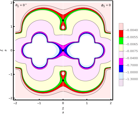
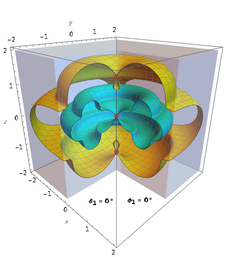
When the polarization of the atom is aligned with the axis of symmetry of the dielectric ring, that is, $\theta_{1}=0$, out of the four projections in Eqs. (6.3) only the projection in Eq. (6.3a) is non-zero. This is an axially symmetric configuration with energy

$$E(z,\rho,0,0)=-E_{0}\frac{2}{\pi}\Bigg[\left(\frac{a^{2}k^{2}}{4a\rho}\right)^{\frac{7}{2}}\pi_{7}(k)\hskip 71.13188pt$$

$$-\frac{56}{13}\frac{z^{2}}{a^{2}}\left(\frac{a^{2}k^{2}}{4a\rho}\right)^{\frac{9}{2}}\pi_{9}(k)+\frac{63}{13}\frac{z^{4}}{a^{4}}\left(\frac{a^{2}k^{2}}{4a\rho}\right)^{\frac{11}{2}}\pi_{11}(k)\Bigg]\hskip 17.07164pt$$ (6.7)

independent of $\theta_{1}$, $\phi_{1}$, and $\phi$. Slices of surfaces of equal energy for the above energy in the $x$-$z$ plane are illustrated as contours in FIG. 3, and this energy in the $z$ direction alone was the blue curve ($\theta_{1}=0$) in FIG. 2. Quadrilobed-toroidal pattern in these surfaces is a signature of the $\cos 2\theta$ dependence of Casimir-Polder interaction energy in contrast to $\cos\theta$ dependence of dipole-dipole interaction energy. Two of the surfaces of equal energy are shown in FIG. 4 in full glory in the complete three dimensional space. Lines normal to these surfaces of equal energy represent the force on the polarizable atom, since it is a conservative force and equal to the negative gradient of energy. Further, the divergence of the force tells us about the stability at a point. This is similar to electrostatics where negative gradient of electric potential is electric field and divergence of electric field at a point is a measure of electric charge density. In electrostatics charge density is a source or sink of electric field. Similarly, Laplacian of energy (in contrast to electric potential) is a source or sink of force, and thus a measure of stability. Thus, in FIG. 3 and FIG. 4, points where the energy surfaces are locally concentric correspond to stable or unstable points and points where the energy surfaces gets pinched and appear as intersecting contours in their cross sections, such as in FIG. 3, are saddle points of equilibrium. Thus, we decipher that the energy in Eq. (6.7) has three equilibrium points on the $z$ axis, one at the origin and one each on either side of the ring on $z$ axis at $z_{0}=\pm 1.3\,a$. We also learn that the unstable points of equilibrium at $z_{0}=\pm 0.96\,a$ appear as hanging blobs in FIG. 4. The force on the atom placed at each of these equilibrium points is zero. We deduce that $z_{0}=\pm 0.96\,a$ is an unstable point of equilibrium because the concentric surfaces are lower in energy going away from this point. For the three saddle points out of the five equilibrium points, energy decreases in in radial directions and energy increases in axial directions. This will be manifested as an attractive force (towards the equilibrium point) in the direction of $z$ and a repulsive force (away from the equilibrium point) in radial directions.

To gain analytical insight into the structure of the energy surface in the neighborhood of the equilibrium points we use the expansion, using Eq. (5.4),

$$\frac{a^{2}k^{2}}{4a\rho}=1-2\frac{\rho}{a}+3\frac{\rho^{2}}{a^{2}}-\frac{z^{2}}{a^{2}}+\dots,$$ (6.8)

in the series expansions for $\pi_{n}(k)$ in Eqs. (4.35) to obtain

$$\left(\frac{a^{2}k^{2}}{4a\rho}\right)^{\frac{7}{2}}\pi_{7}(k)=\frac{\pi}{2}\left[1+\frac{49}{4}\frac{\rho^{2}}{a^{2}}-\frac{7}{2}\frac{z^{2}}{a^{2}}+\ldots\right],$$ (6.9)

and

$$\frac{z^{2}}{a^{2}}\left(\frac{a^{2}k^{2}}{4a\rho}\right)^{\frac{9}{2}}\pi_{9}(k) = \frac{z^{2}}{a^{2}}\frac{\pi}{2}+\ldots,$$ (6.10a)

$$\frac{z^{4}}{a^{4}}\left(\frac{a^{2}k^{2}}{4a\rho}\right)^{\frac{11}{2}}\pi_{11}(k) = 0+\ldots,$$ (6.10b)

which yields the form of energy in the vicinity of the equilibrium point at the origin to be

$$z_{0}=0:\hskip 8.53581ptE=-E_{0}\left[1+\frac{49}{4}\frac{\rho^{2}}{a^{2}}-\frac{203}{26}\frac{z^{2}}{a^{2}}+\ldots\right].$$ (6.11)

The overall negative coefficient for $\rho^{2}$ implies a negative second derivative thus instability in radial directions and a positive coefficient for $z^{2}$ implies stability in axial directions.

Figure 5: Each of the frames show cross sections of surfaces of equal energy in Eq. (5.22) as contours in the region of space surrounding the unipolarizable dielectric ring of radius $a$ as a function of position $\rho$ and $z$ of the unipolarizable atom. The cross section in each frame is the $x$-$z$ plane. Each of the nine frames correspond to a fixed azimuth angle $\phi_{1}=0^{\circ}$ of the polarizability of atom, and the variation in the frames is in the orientation angle $\theta_{1}$ of the polarizability. The frame on the top left, for $\theta_{1}=0^{\circ}$, has three saddle points of equilibrium described by black dots, one at the origin and two (one on each side of ring) on the $z$ axis at $z_{0}=\pm 1.3\,a$. These three equilibrium points drift away from the $z$ axis as we change the orientation of the polarizability of the atom in the following frames for angles $\theta_{1}=0^{\circ},30^{\circ},45^{\circ},60^{\circ},90^{\circ},$ and then for $\theta_{1}=180^{\circ},150^{\circ},135^{\circ},120^{\circ},90^{\circ}$. The legend for the contours is energy measured in units of $E_{0}$, that is, $E/E_{0}$. The contours show an inversion symmetry about the origin between orientations $90^{\circ}<\theta_{1}<180^{\circ}$ and $0^{\circ}<\theta_{1}<90^{\circ}$.

Figure 6: Each of the frames show two surfaces of equal energy in Eq. (5.22) in the region of space surrounding the unipolarizable dielectric ring of radius $a$ as a function of position of the unipolarizable atom. The variables on the axes, $x$, $y$, and $z$, represent the position of the polarizable atom and are in multiples of radius $a=1$ of ring. Each of the nine frames correspond to a fixed azimuth angle $\phi_{1}=0^{\circ}$ of the polarizability of atom, and the variation in the frames is in the orientation angle $\theta_{1}$ of the polarizability. The equilibrium points are described by red dots. The center of the ring is a saddle point of equilibrium except when $\theta_{1}=90^{\circ}$. Orientations for $90^{\circ}<\theta_{1}<180^{\circ}$ is identical to $0^{\circ}<\theta_{1}<90^{\circ}$ with an inversion symmetry about the origin. The (outer) yellow colored surface for each $\theta_{1}$ is the energy surface that passes through two (one on each side of ring) saddle points of equilibrium, with energies $E=-E_{0}(0.0065,0.0063,0.0063,0.004,0.004)$ for angles $\theta_{1}=0^{\circ},30^{\circ},45^{\circ},60^{\circ},90^{\circ},$ and the same for $\theta_{1}=180^{\circ},150^{\circ},135^{\circ},120^{\circ},90^{\circ},$. The (inner) cyan colored surface are the energy surfaces that contains the saddle points of equilibrium closer to the ring with energies $E=-E_{0}(1,0.75,0.5,0.16,0.178)$ for angles $\theta_{1}=0^{\circ},30^{\circ},45^{\circ},60^{\circ},90^{\circ},$ and the same for $\theta_{1}=180^{\circ},150^{\circ},135^{\circ},120^{\circ},90^{\circ}$.

Similar series expansions in the neighborhood of the five equilibrium points discussed above, keeping until quadratic terms, are

$$\frac{z_{0}}{a} =0: \frac{E}{E_{0}} =-1-12\frac{\rho^{2}}{a^{2}}+7.8\frac{\tilde{z}^{2}}{a^{2}},$$ (6.12a)

$$\frac{z_{0}}{a} =\pm 0.96: \frac{E}{E_{0}} =-0.0050-0.11\frac{\rho^{2}}{a^{2}}-0.097\frac{\tilde{z}^{2}}{a^{2}},$$ (6.12b)

$$\frac{z_{0}}{a} =\pm 1.3: \frac{E}{E_{0}} =-0.0065-0.61\frac{\rho^{2}}{a^{2}}+0.024\frac{\tilde{z}^{2}}{a^{2}},$$ (6.12c)

where

$$\tilde{z}=z-z_{0}$$ (6.13)

are deviations from respective equilibrium points $z_{0}$ given in units of ring radius $a$. The relative signs and values of the coefficients of $\rho^{2}$ and $z^{2}$ terms reveal the nature of the equilibrium points. Thus, we infer, again, that $z_{0}=\pm 1.3\,a$ and $z_{0}=0$ are saddle points of equilibrium and $z_{0}=\pm 0.96\,a$ are unstable points of equilibrium. The force on the polarizable atom in the vicinity of these equilibrium points is evaluated using

$${\bf F}=-{\bm{\nabla}}E,$$ (6.14)

in terms of $F_{0}=E_{0}/a$ as

$$\frac{z_{0}}{a} =0: {\bf F} =F_{0}\left[24\frac{\rho}{a}\hat{\bm{\rho}}-16\frac{\tilde{z}}{a}\hat{\bf z}\right],$$ (6.15a)

$$\frac{z_{0}}{a} =\pm 0.96: {\bf F} =F_{0}\left[0.22\frac{\rho}{a}\hat{\bm{\rho}}+0.19\frac{\tilde{z}}{a}\hat{\bf z}\right],$$ (6.15b)

$$\frac{z_{0}}{a} =\pm 1.3: {\bf F} =F_{0}\left[0.12\frac{\rho}{a}\hat{\bm{\rho}}-0.048\frac{\tilde{z}}{a}\hat{\bf z}\right],$$ (6.15c)

each of which is easily verified to be zero at the respective equilibrium points. It is known that the stability or instability at these equilibrium points is not conclusively measured by the divergence of force, the Laplacian of the negative of energy [27]. The divergence of force at the equilibrium points are

$$\frac{z_{0}}{a} =0: \frac{{\bm{\nabla}}\cdot{\bf F}}{(F_{0}/a)} =(48-16)=32,$$ (6.16a)

$$\frac{z_{0}}{a} =\pm 0.96: \frac{{\bm{\nabla}}\cdot{\bf F}}{(F_{0}/a)} =(0.44+0.19)=0.63,$$ (6.16b)

$$\frac{z_{0}}{a} =\pm 1.3: \frac{{\bm{\nabla}}\cdot{\bf F}}{(F_{0}/a)} =(0.24-0.048)=0.19,$$ (6.16c)

where a multiplicative factor of 2 in the $\rho$ directions is due to the contribution from the angular dependence in $\hat{\bm{\rho}}$. That is, ${\bm{\nabla}}\cdot(\rho\hat{\bm{\rho}})=2$. Thus, deducing that $z_{0}=\pm 0.96\,a$ is an unstable equilibrium point in this manner is not conclusive but consistent with the inference made earlier using graphical analysis. For completeness, we also verify that

$${\bm{\nabla}}\times{\bf F}=0$$ (6.17)

at each of the above equilibrium points. We also point out that the yellow outer surface in FIG. 4 on which four of the five equilibrium points reside are about hundred times smaller in energy relative to the cyan inner surface. Thus, the valley constituting the saddle points are shallow and probably not very easily accessible for applications. Nevertheless, the features in the energy landscape are insightful.

We can extend the analysis of each of the equilibrium points for orientation $\theta_{1}=0^{\circ}$ as we change the orientation. This is summarized adequately by showing the drift of these equilibrium points as a function of orientation angle. This has been summarized in Tables 1 and 2 and has been illustrated in FIG. 7. The equilibrium points are of course just the highlights of the energy surfaces in FIGs. 5 and 6. The contours in FIGs. 5 are curves that represent cross sections in the $x$-$z$ plane of equal energy surfaces. The complete surface (which the curves in FIGs. 5 are part of) are shown in FIG. 6. The specific energy surfaces we have have displayed for each of the orientations are those that contain equilibrium points, or are in close vicinity of these surfaces. This graphical display is crucial for investigating the stability of the equilibrium points. We mention that concrete analytical methods to investigate the stability of equilibrium points in three dimensions are lacking and graphical analysis is the tool-of-choice. The basics of graphical stability analysis is to look for concentric surfaces around an equilibrium point representing stability or instability in all three directions and for conical intersections in the energy surfaces representing instability in at least one of the three directions. This is similar to the analysis described in Ref. [27], though in a different context. The intersections displayed in FIGs. 5 and 6 were determined by manually searching for the specific energy. This was a tedious affair, but can be easily automated if it has to be done at a bigger scale. Data for each frame in FIG. 5 took about five minutes to be generated on a typical PC, and data for each frame in FIG. 6 was generated in about five hours.

Figure 7: Drift of position $(x_{e},y_{e},z_{e})$ of equilibrium points on equal energy surfaces for the energy in Eq. (6.7) as a function of the orientation of the polarization $(\theta_{1},\phi)$ of the unipolarizable atom. The blue dots are graphical representations of the data in Table 1 that are absent for $33^{\circ}<\theta_{1}<147^{\circ}$, and red dots are graphical representations of the data in Table 2 that are absent for $\theta_{1}<55^{\circ}$ and $125^{\circ}<\theta_{1}$. The equilibrium point at origin does not drift.

$(\theta_{1},\phi_{1})$		$(x_{e},y_{e},z_{e})$		$E$
$(0^{\circ},0^{\circ})$		$(0.00\,a,0,1.3\,a)$		$-0.0065\,E_{0}$
$(15^{\circ},0^{\circ})$		$(0.14\,a,0,1.2\,a)$		$-0.0064\,E_{0}$
$(30^{\circ},0^{\circ})$		$(0.29\,a,0,1.2\,a)$		$-0.0063\,E_{0}$
$(32^{\circ},0^{\circ})$		$(0.32\,a,0,1.2\,a)$		$-0.0063\,E_{0}$
$(33^{\circ},0^{\circ})$		$(0.33\,a,0,1.1\,a)$		$-0.0063\,E_{0}$
$(147^{\circ},0^{\circ})$		$(-0.33\,a,0,1.1\,a)$		$-0.0063\,E_{0}$
$(148^{\circ},0^{\circ})$		$(-0.32\,a,0,1.2\,a)$		$-0.0063\,E_{0}$
$(150^{\circ},0^{\circ})$		$(-0.29\,a,0,1.2\,a)$		$-0.0063\,E_{0}$
$(165^{\circ},0^{\circ})$		$(-0.14\,a,0,1.2\,a)$		$-0.0064\,E_{0}$
$(180^{\circ},0^{\circ})$		$(0.00\,a,0,1.3\,a)$		$-0.0065\,E_{0}$

Table 1: Position of equilibrium point at $(x_{e},y_{e},z_{e})$ that originates at $(0,0,\pm 1.3\,a)$ on equal energy surfaces for the energy $E$ in Eq. (6.7) as a function of the orientation of the polarization $(\theta_{1},\phi_{1})$ of the unipolarizable atom. This equilibrium point is absent for $33^{\circ}<\theta_{1}<147^{\circ}$.

$(\theta_{1},\phi_{1})$		$(x_{e},y_{e},z_{e})$		$E$
$(55^{\circ},0^{\circ})$		$(-0.17\,a,0,0.37\,a)$		$-0.16\,E_{0}$
$(57^{\circ},0^{\circ})$		$(-0.14\,a,0,0.40\,a)$		$-0.16\,E_{0}$
$(60^{\circ},0^{\circ})$		$(-0.12\,a,0,0.42\,a)$		$-0.16\,E_{0}$
$(75^{\circ},0^{\circ})$		$(-0.05\,a,0,0.46\,a)$		$-0.17\,E_{0}$
$(90^{\circ},0^{\circ})$		$(0,0,0.47\,a)$		$-0.18\,E_{0}$
$(105^{\circ},0^{\circ})$		$(0.05\,a,0,0.46\,a)$		$-0.17\,E_{0}$
$(120^{\circ},0^{\circ})$		$(0.12\,a,0,0.42\,a)$		$-0.16\,E_{0}$
$(123^{\circ},0^{\circ})$		$(0.14\,a,0,0.40\,a)$		$-0.16\,E_{0}$
$(125^{\circ},0^{\circ})$		$(0.17\,a,0,0.37\,a)$		$-0.16\,E_{0}$

Table 2: Position of equilibrium point at $(x_{e},y_{e},z_{e})$ that originates at $(0,0,\pm 0.47\,a)$ on equal energy surfaces for the energy $E$ in Eq. (6.7) as a function of the orientation of the polarization $(\theta_{1},\phi_{1})$ of the unipolarizable atom. This equilibrium point is absent for $\theta_{1}<55^{\circ}$ and $125^{\circ}<\theta_{1}$.

When the polarization of the atom is perpendicular to the axis of symmetry of the dielectric ring, that is, $\theta_{1}=90^{\circ}$, and if $\phi_{1}-\phi=0$, then out of the four projections in Eqs. (6.3) only the projection in Eq. (6.3b) is non-zero. The energy for this configuration is

$$E(z,\rho,90^{\circ},0)=-E_{0}\frac{63}{13}\frac{z^{2}}{a^{2}}\left(\frac{a^{2}k^{2}}{4a\rho}\right)^{\frac{11}{2}}\frac{2}{\pi}\Bigg[\frac{4}{k^{4}}\pi_{7}(k)\hskip 28.45274pt$$

$$+\frac{4}{k^{2}}\left(1+\frac{\rho}{a}-\frac{2}{k^{2}}\right)\pi_{9}(k)+\left(1+\frac{\rho}{a}-\frac{2}{k^{2}}\right)^{2}\pi_{11}(k)\Bigg].\hskip 19.91692pt$$ (6.18)

For finding series expansions around equilibrium points it is convenient to rewrite it in the form

$$E(z,\rho,90^{\circ},0) = -E_{0}\frac{63}{13}\frac{z^{2}}{a^{2}}\left(\frac{a^{2}k^{2}}{4a\rho}\right)^{\frac{11}{2}}\frac{2}{\pi}\hskip 28.45274pt$$ (6.19)

$$\times\Bigg[c_{1}(k)+2\frac{\rho}{a}c_{2}(k)+\frac{\rho^{2}}{a^{2}}\pi_{11}(k)\Bigg],\hskip 19.91692pt$$

where $c_{1}(k)$ is given by the expression in Eq. (5.18a) and $c_{2}(k)$ is given by the expression in Eq. (5.18c). The expansions of energy in the vicinity of the three equilibrium points are

$$\frac{z_{0}}{a} =0: \frac{E}{E_{0}} =0-2.4\frac{\tilde{z}^{2}}{a^{2}}-68\frac{\rho^{2}}{a^{2}}\frac{\tilde{z}^{2}}{a^{2}},$$ (6.20a)

$$\frac{z_{0}}{a} =\pm 0.47: \frac{E}{E_{0}} =-0.18+1.3\frac{\tilde{z}^{2}}{a^{2}}-2.8\frac{\rho^{2}}{a^{2}}\frac{\tilde{z}^{2}}{a^{2}}.$$ (6.20b)

An animation illustrating the variation in the energy surfaces including the drift of equilibrium points as a function of polarization of the unipolarizable atom is available in Ref. [31] as a supplementary material. The geometrical shape of energy surfaces can be understood in the following manner. The equal energy surfaces of a point electric charge are concentric spheres. The equal energy surfaces of point electric dipole are bilobal, each lobe with opposite sign of energy. The equal energy surfaces of a polarizable particle are quadrilobal, that is, has four lobes, with all four lobes having the same sign of energy. A polarizable ring has equal energy surface in the shape of a toroid with the cross section of the channel constituting the toroid having the shape of a quadrilobe. If we imagine the quadrilobe-toroidal shaped energy surface to be constructed by stretching and compressing the energy surface of a line of polarizable particles, we can imagine the surfaces to be squeezed near the center of the ring. This energy surface has to coexist by topologically transforming itself to accommodate the quadrilobe of a polarizable atom. This interpretation is consistent with the energy surfaces in FIGs. 5 and 6.

7 Conclusion and Outlook

We presented an exact expression for the Casimir-Polder interaction energy between a unipolarizable atom and a unipolarizable dielectric ring in terms of elliptic integrals in Eq. (5.22). The qualitative features of the results associated to the equilibrium points on the $z$ axis were already known in literature. The quantitative analysis of stability at the equilibrium points, both on the axis and off the axis, are new. The exact analytic expression for energy allows us to find quadratic approximation of the same in the vicinity of equilibrium points, that in turn allows us to investigate the nature of stability at these equilibrium points. Contours of equal energy surfaces, not to be confused with electric equipotential surfaces, are used to analyze stability. Conical intersections in energy surfaces represent saddle points and concentric surfaces imply stable or unstable points. This procedure will be useful to investigate feasibility of designs for stabilizing and thus trapping an atom in interactions based on vacuum fluctuations.

Earnshaw theorem in electrostatics states that stable equilibrium points are not possible in static configurations. Thus, surfaces of equal energy for a static charge configuration will not allow for concentric surfaces in a region such that the inner surfaces are lower in energy relative to the outer. For example, for the case of a point magnet interacting with a ring magnet the equilibrium points are always saddle points, that is, it is unstable in at least one direction out of three and the intersections in energy surfaces are conical [30]. Earnshaw theorem is well known to be not applicable for non-static configurations. For example, a spinning magnet can levitate above a ring magnet, like a Levitron${}^{\text{TM}}$ [5]. Similarly, electromagnets with alternating current can levitate magnets. In light of these examples we should not expect Earnshaw theorem to hold for interactions manifested by vacuum fluctuations because they are inherently dynamic. Thus, stability analysis in Casimir-Polder interactions with a likelihood for a violation of Earnshaw theorem is warranted. Earnshaw theorem has been discussed for polarizable atoms in Ref. [2] and for vacuum fluctuations induced interactions in Ref. [24]. Unlike the case of a point magnet interacting with a ring magnet [30] where we only see conical intersections in energy surfaces, our analysis here suggests that we can find equilibrium points with locally concentric energy surfaces around it in Casimir-Polder interactions. See, for example, $\theta_{1}=0$ case around $z=\pm 0.96\,a$ and $\rho=0$, which appears as a hanging blob in FIG. 3 with concentric surfaces inside the blob. These equilibrium points lead to instability in all three directions. This observation is new and leads to the question if it is possible to have such concentric surfaces such that the equilibrium points lead to stability. This motivates us to inquire if there are subtle differences in the statement of Earnshaw theorem in the context of vacuum fluctuations.

In molecular chemistry it is known that equal energy surfaces for two atoms do not intersect if the interatomic distance is the only parameter in the energy [29]. However, if the energy depends on additional parameters, like the orientation of the dipole-moments of the atoms, then the energy surfaces accommodates conical intersections [27]. It has been further shown that the spatial degeneracy in energy causes the molecules to distort, the Jahn-Teller effect [15]. Extending these ideas from molecular chemistry to Casimir-Polder interactions is promising. We could inquire if a distortion in the polarizability of the ring could inherently change the nature of equilibrium points. A distortion that is presumably tractable is a configuration where the polarizability of the ring, $\sigma_{2}\,\hat{\bf m}\hat{\bf m}$, is non-uniform along the ring,

$$\hat{\bf m}=\cos\phi\,\hat{\bf z}+\sin\phi\,\hat{\bm{\rho}}.$$ (7.1)

Qualitatively, we can imagine a quadrilobed-toroidal pattern, which is a useful picturization of a polarizable atom, to be twisting and turning once as it loops and forms a ring. The effect this azimuthal asymmetry has on the interaction energy and the associated equilibrium points would suggest a Jahn-Teller effect in Casimir-Polder interactions at macroscopic scale in contrast to molecular scale.

8 acknowledgments

We thank Dinuka Gallaba and Duston Wetzel for collaborative assistance. KVS thanks Bumsu Lee and Punit Kohli at SIUC for discussions.

References

- [1] (2018-07) Repulsive van der Waals interaction between a quantum particle and a conducting toroid. Phys. Rev. A 98, pp. 012511. Cited by: §1.
- [2] (1978-03) Trapping of Atoms by Resonance Radiation Pressure. Phys. Rev. Lett. 40, pp. 729. Cited by: §7.
- [3] (1943) Interaction of the van der Waals type between three atoms. J. Chem. Phys. 11 (6), pp. 299. Cited by: §1.
- [4] (2005) Long-range atom-surface interactions for cold atoms. J. Phys. Conf. Ser. 19 (1), pp. 1. Cited by: §1.
- [5] (1996) The Levitron: an adiabatic trap for spins. Proc. R. Soc. Lond. A. 452 (1948), pp. 1207. Cited by: §7.
- [6] (1971) Handbook of elliptic integrals for engineers and scientists. 2 edition, Springer Verlag, Berlin. Cited by: §4, §4, §4, §4, §4.
- [7] (1948) On the attraction between two perfectly conducting plates. Kon. Ned. Akad. Wetensch. Proc. 51, pp. 793. Cited by: §1.
- [8] (1969) The asymptotic Casimir-Polder potential for anisotropic molecules. Chem. Phys. Lett. 3 (4), pp. 195. Cited by: §1.
- [9] (1969) The asymptotic Casimir-Polder potential from second-order perturbation theory and its generalization for anisotropic polarizabilities. Int. J. Quantum Chem. 3 (6), pp. 903. Cited by: §1.
- [10] NIST Digital Library of Mathematical Functions. Note: Release 1.0.8 of 2014-04-25Online companion to [23] Cited by: §4, 23.
- [11] (2011-05) Casimir-Polder interaction between a polarizable particle and a plate with a hole. Phys. Rev. A 83, pp. 052514. Cited by: §1.
- [12] (1930) Über das Vrhältnis der van der Waalsschen Kräfte zu den Homöopolaren Bindungskräften. Z. Physik 60, pp. 491. Note: English translation in [14] Cited by: §1.
- [13] (1910) Lectures on the theory of elliptic functions. Vol. 1, John Wiley & Sons, New York. Cited by: §4, §4.
- [14] (2000) Quantum chemistry: Classic scientific papers. World Scientific Series in 20th century chemistry, World Scientific. Cited by: §1, 12, 17.
- [15] (1937-07) Stability of polyatomic molecules in degenerate electronic states - I—Orbital degeneracy. Proc. R. Soc. A 161 (905), pp. 220. Cited by: §7.
- [16] (2010) Casimir repulsion between metallic objects in vacuum. Phys. Rev. Lett. 105, pp. 090403. External Links: Document Cited by: §1, §3.
- [17] (1930) Zur Theorie und Systematik der Molekularkräfte. Z. Physik 63, pp. 245. Note: English translation in [14] Cited by: §1.
- [18] (2020) Geometrical dependence in Casimir-Polder repulsion: Anisotropically polarizable atom and anisotropically polarizable annular dielectric. arXiv 2011.11871. Cited by: §1, §1, §2, §3, §6, §6.
- [19] (2021-09) Geometrical dependence in Casimir-Polder repulsion. Phys. Rev. A 104, pp. 032209. Cited by: §1, §1, §1.
- [20] (2012-01) Casimir-Polder repulsion: Polarizable atoms cylinders, spheres, and ellipsoids. Phys. Rev. D 85, pp. 025008. Cited by: §1.
- [21] (2008-10) Exact Results for Casimir Interactions between Dielectric Bodies: The Weak-Coupling or van der Waals Limit. Phys. Rev. Lett. 101, pp. 160402. Cited by: §5.
- [22] (1943) . J. Phys. Math. Soc. Japan 17, pp. 629. External Links: Document Cited by: §1.
- [23] (2010) NIST handbook of mathematical functions. Note: Edited by F. W. J. Olver and D. W. Lozier and R. F. Boisvert and C. W. Clark. Print companion to [10] Cited by: 10.
- [24] (2010-08) Constraints on stable equilibria with fluctuation-induced (Casimir) forces. Phys. Rev. Lett. 105, pp. 070404. Cited by: §7.
- [25] (2012) Repulsive long-range forces between anisotropic atoms and dielectrics. Phys. Rev. A 85, pp. 012523. Cited by: §1.
- [26] (2011) Observation of the thermal Casimir force. Nature Phys. 7, pp. 230. Cited by: §5.
- [27] (1937) The Crossing of Potential Surfaces. J. Phys. Chem. 41 (1), pp. 109. Cited by: §6, §6, §7.
- [28] (1873) Over de Continuiteit van den Gas-en Vloeistoftoestand, (On the continuity of the gas and liquid state). Ph.D. Thesis, Universiteit Leiden (Leiden University), The Netherlands. Cited by: §1.
- [29] (1929) Uber merkwurdige diskrete eigenwerte. uber das verhalten von eigenwerten bei adiabatischen prozessen. Physik. Z. 30, pp. 467. Cited by: §7.
- [30] (2023) Magnetostatic interaction energy between a point magnet and a ring magnet. Physics Open 15, pp. 100140. Cited by: §1, §4, §7.