A Joint Variational Framework for Multimodal X-ray Ptychography and Fluorescence Reconstruction

Abstract

Recovering high-resolution structural and compositional information from coherent X-ray measurements involves solving coupled, nonlinear, and ill-posed inverse problems. Ptychography reconstructs a complex transmission function from overlapping diffraction patterns, while X-ray fluorescence provides quantitative, element-specific contrast at lower spatial resolution. We formulate a joint variational framework that integrates these two modalities into a single nonlinear least-squares problem with shared spatial variables. This formulation enforces cross-modal consistency between structural and compositional estimates, improving conditioning and promoting stable convergence. The resulting optimization couples complementary contrast mechanisms (i.e., phase and absorption from ptychography, elemental composition from fluorescence) within a unified inverse model. Numerical experiments on simulated data demonstrate that the joint reconstruction achieves faster convergence, sharper and more quantitative reconstructions, and lower relative error compared with separate inversions. The proposed approach illustrates how multimodal variational formulations can enhance stability, resolution, and interpretability in computational X-ray imaging.

65J22, 90C06, 68U10

1 Introduction

Ptychography has matured into a coherent X-ray microscopy technique in which a focused beam is scanned across the specimen with deliberate overlap while a pixelated detector records far-field diffraction intensities [20]. Inverting these phaseless data recovers the specimen’s complex transmission function, enabling quantitative, nanometer-scale imaging across domains from biology to battery materials [29, 27]. Besides the wide application of ptychographic imaging, its reconstruction remains as a challenging problem due to its nonlinear and nonconvex nature, such as the symmetries that create non-uniqueness. Classical solvers, including alternating projections and constraint algorithms [3, 13, 4], ptychographical iterative engine-family (PIE) updates [21, 16], and maximum-likelihood/variational and Wirtinger-gradient methods [10, 19], can converge rapidly when well initialized, but are susceptible to stagnation and local minima, especially with weak overlap, low counts, or model mismatch.

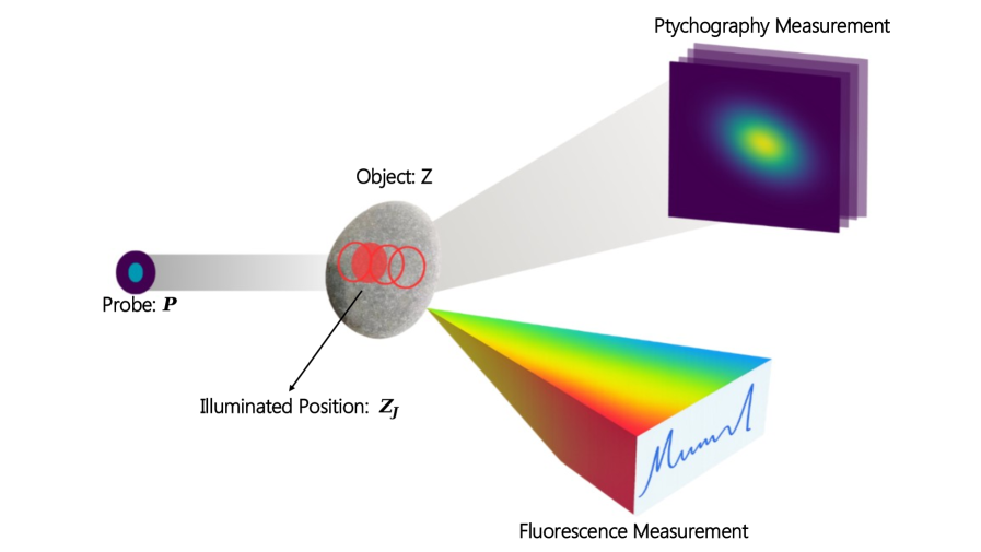
Complementary contrast is provided by X-ray fluorescence (XRF) [2], which detects element-specific secondary emission photons that are released when incident X-rays excite core electrons. Because each element emits a unique set of characteristic lines, XRF yields quantitative maps of elemental composition and trace distribution, even at very low concentrations. The drawback is that the emitted photons originate from the entire illuminated volume, so the recorded fluorescence map is effectively the convolution of the true elemental distribution with the probe intensity profile used during scanning. This convolution blurs fine details and constrains the resolution of fluorescence images to the probe size and scan step, even though the data themselves contain chemically specific information. When ptychographic and fluorescence measurements are collected simultaneously, the ptychographic reconstruction delivers an accurate, high-resolution estimate of the probe function. That probe can then be used as a deconvolution kernel for the fluorescence signal, allowing one to invert the blurring process and recover fluorescence maps with substantially improved resolution—sometimes exceeding the nominal probe width and approaching super-resolution. In this way, the two modalities are naturally complementary: ptychography provides quantitative phase and structural sensitivity, while XRF supplies element-specific chemical contrast. These complementary strengths naturally call for a joint inverse formulation that coherently leverages both datasets. The joint experiment process is illustrated in Figure 1.

Figure 1: An illustration of a joint ptychographic and fluorescence experiment.

An early demonstration at synchrotrons combined X-ray ptychography with XRF in a single scan: ptychography supplied high-resolution complex transmission function while XRF provided element maps; using the reconstructed probe as a point-spread function enabled deconvolution that sharpened fluorescence beyond the optics-limited resolution and contextualized elemental distributions in a biological specimen [28, 7]. Di et al. [8] proposed a nonlinear optimization–based joint inversion framework that integrates XRF with X-ray transmission data to reconstruct elemental distributions while simultaneously modeling attenuation and self-absorption, thereby reducing the ill-posedness compared with XRF-only reconstructions. This work established the joint model and solution strategy; subsequent work [9] extended it to joint XRF and transmission tomography, showing improved quantitative accuracy and mitigation of spectral mixing and self-absorption on simulated and experimental datasets. In parallel, the electron-microscopy community advanced closely related ideas. Schwartz et al. [25, 24] framed fused multi-modal electron microscopy as a constrained optimization that links elastic scattering with inelastic scattering, yielding chemical maps with substantially higher signal-to-noise ratio and enabling 10x dose reductions while providing uncertainty estimates from the Hessian. These existing work underscores a general principle for multimodal fusion: tying modalities through a physics-based objective can trade information across channels to achieve low-dose, quantitative chemical imaging at (sub-)nanometer scales.

In this study, we propose a new joint reconstruction framework that explicitly integrates ptychographic and XRF measurements through a link function. The central idea is to treat the two modalities not as separate post-processing steps, but as coupled observations of the same underlying object: the complex transmission function governs the ptychographic phase contrast, while the elemental composition drives the fluorescence emission. By embedding these relationships into a single inverse problem, our method leverages the structural sensitivity of ptychography and the elemental specificity of XRF in a mutually reinforcing way. The link function enforces physical consistency between the modalities, so that each modality regularizes the other within a single optimization framework. The cross-modal coupling improves the conditioning of the otherwise ill-posed inverse problems, suppresses noise and model mismatch, and yields reconstructions with enhanced quantitative accuracy compared to single-modal analyses.

2 Joint formulation

To establish the proposed joint reconstruction framework, we begin by reviewing the mathematical models underlying each imaging modality. This provides the foundation for formulating a unified loss that couples ptychography and fluorescence data.

2.1 Mathematical background

In $2$D ptychographic phase retrieval, the goal is to reconstruct the complex transmission function of an object $z=x+yi=|z|e^{i\phi}\in\mathbb{C}^{n\times n}$ from its observed diffraction pattern, where $\phi$ is the phase of the object. The data $d_{j}\in\mathbb{R}^{m\times m}$ is collected as phaseless intensity measurements from the $\text{j}^{\text{th}}$ scanning position and $d=\{d_{j}\}_{j=1}^{N}\in\mathbb{R}^{m\times m\times N}$ is the collection of intensity measurements at all $N$ scanning positions. A ptychography experiment for one scanning position is modeled by

$$d_{j}=\big|\mathcal{F}(P\odot z_{j})\big|^{2}+\epsilon_{j},\quad j=1,\cdots,N,$$

where $\odot$ denotes element-wise matrix multiplication. The operator $\mathcal{F}:\mathbb{C}^{m\times m}\to\mathbb{C}^{m\times m}$ is the two-dimensional discrete Fourier transform, and $|\cdot|^{2}:\mathbb{C}^{m\times m}\to\mathbb{R}^{m\times m}$ computes element-wise intensity. The sub-matrix $z_{j}\in\mathbb{C}^{m\times m}$ corresponds to the sub-region of $z$ being illuminated at the $j$-th scanning position. $P\in\mathbb{C}^{m\times m}$ denotes the complex probe. Finally, $\epsilon_{j}\in\mathbb{R}^{m\times m}$ models the noise in the $j$-th measurement.

The overlap ratio quantifies how much the probe’s illuminated footprint at one scan position overlaps the footprint at a neighboring position. Practically, it is reported relative to an effective probe width (e.g., full width at half maximum): a “50% overlap” means the scan step is about half the probe width along the scan axes. Increasing the overlap increases data redundancy and improves the conditioning of the ptychographic forward operator, which generally enlarges the basin of convergence and makes reconstructions more robust to noise and position/probe errors—albeit at the cost of longer acquisitions and dose. In practice, approximately 60–80% overlap is commonly used for reliable reconstructions [17].

There are different ways of formulating the ptychographic reconstruction problem [11]. One such formulation we focus on in this work is the amplitude-based error metric:

$$\min_{P,z}\Phi^{\text{ptyc}}(P,z)=\frac{1}{2N}\sum_{j=1}^{N}\left\||\mathcal{F}(P\odot z_{j})|-\sqrt{d_{j}}\right\|_{2}^{2},$$

where the absolute value operator $|\cdot|$ makes the optimization problem nonlinear.

On the other hand, we model the expected fluorescence counts for element $e$ as a non-blind deconvolution with a known excitation Point Spread Function (PSF) given by the probe intensity

(1) $$\min_{w,P}\;\Phi^{\text{fluor}}(P,w)\;=\;\min_{w,P}\frac{1}{2N_{e}}\sum_{e=1}^{N_{e}}\left\|\,|P|^{2}\ast w_{e}-D_{e}\,\right\|_{2}^{2},$$

where $\ast$ denotes the convolution operator, $w_{e}\in\mathbb{R}^{n\times n}$ is the expected high resolution elemental map, and $w=[w_{e}]_{e=1}^{N_{e}}$ is the collection of $N_{e}$ XRF elemental maps. The loss is then computed against $D_{e}\in\mathbb{R}^{n\times n}$, the experimentally measured fluorescence intensity map for element $e$.

2.2 Joint reconstruction formulation

To enhance ptychographic reconstructions under limited data, we integrate fluorescence information by introducing a lightweight, physics-guided coupling between the object’s imaginary component $y$ and its linear attenuation coefficient $\mu$. Let $\mu_{e}^{E_{0}}$ be the mass attenuation coefficient at the incident energy $E_{0}$. Under a thin‑sample/single‑scatter model,

$$\mu\;=\;\sum_{e=1}^{N_{e}}\mu_{e}^{E_{0}}\,w_{e}.$$

For the sake of a simple cross-modal link, we use $y$ (i.e., the imaginary term of the object $z$) as a surrogate for attenuation. Physically, attenuation is encoded in the magnitude of the transmission function $|z|=e^{-\frac{1}{2}\int\mu dt}$, with $z=e^{-a}e^{i\phi}$ and $a=-\log|z|$, rather than in $y$ alone. To keep the coupling lightweight, we exploit the global phase gauge of ptychography to apply a constant rotation $z\mapsto\tilde{z}=e^{-i(\bar{\phi}+\pi/2)}z$, after which, under a weak-contrast linearization $(|a|\ll 1,\ |\phi-\bar{\phi}|\ll 1)$, the rotated imaginary part satisfies $\tilde{y}\approx-e^{-a}\approx-(1-a)$. We therefore treat (a normalized, sign-adjusted) $y$ as a monotone proxy for the line-integrated attenuation, calibrating an affine map from $y$ to $a$ using vacuum/background regions or a thin standard. This approximation avoids log-amplitude transforms and simplifies the joint objective, and is adequate for prototyping algorithmic structure and ablations. Its limitations are clear: the performance degrades when phase variations are large, when the weak-object assumption fails, or for thick/strongly scattering samples. In subsequent work and for quantitative results, we will replace this proxy with the physically accurate link and, where needed, a multislice/attenuation-path model.

Thus, explicitly bridging these two modalities, we introduce a link function that substitutes the absorption term $\mu$ by $y$ in the ptychographic model with the weighted sum of elemental maps:

$$y=\sum_{e=1}^{N_{e}}\mu_{e}w_{e}.$$

This link function is crucial: it ensures that both modalities share a consistent representation of absorption, thereby coupling the elemental concentration maps with the ptychographic reconstruction. As a result, the two previously independent loss terms, fluorescence data fidelity and ptychographic data fidelity, are unified into a single joint objective. Specifically, we obtain

$$\min_{w,P,x}\frac{\alpha}{2N_{e}}\sum_{e=1}^{N_{e}}\bigl\|\,|P|^{2}\ast w_{e}-D_{e}\bigr\|_{2}^{2}+\frac{1}{2N}\sum_{j=1}^{N}\bigl\|\,|\mathcal{F}\bigl(P\odot(x+i\sum_{e=1}^{N_{e}}\mu_{e}w_{e})_{j}\bigr)|-\sqrt{d_{j}}\bigr\|_{2}^{2},$$

where $\alpha$ balances the contribution of the two modalities.

For simplicity and identifiability, we restrict this work to the non-blind case, where the probe $P$ is assumed to be known and fixed:

(2) $$\min_{w,x}\frac{\alpha}{2N_{e}}\sum_{e=1}^{N_{e}}\bigl\|\,|P|^{2}\ast w_{e}-D_{e}\bigr\|_{2}^{2}+\frac{1}{2N}\sum_{j=1}^{N}\bigl\|\,|\mathcal{F}\bigl(P\odot(x+i\sum_{e=1}^{N_{e}}\mu_{e}w_{e})_{j}\bigr)|-\sqrt{d_{j}}\bigr\|_{2}^{2}.$$

2.3 Optimal choice of alpha

We determine $\alpha$ in (2) using the GradNorm strategy [6]. In GradNorm, the desired gradient norm for each task $i$ is modeled as

$$G_{i}(z)\;=\;\overline{G(z)}\,\times\,[r_{i}(z)]^{\beta},$$

where $G_{i}$ denotes the gradient norm of task $i$, $\overline{G(z)}$ is the average gradient norm across all tasks, and $r_{i}(z)$ represents the relative loss of task $i$. Under this formulation, the task-specific weights $\alpha_{i}$ are chosen such that

$$G_{i}\cdot\alpha_{i}\;=\;\overline{G(z)},$$

thereby ensuring that each weighted gradient matches the average gradient norm. Since our joint model involves only two components, we reduce the GradNorm weighting scheme to a single scalar parameter $\alpha$. At initialization, we set

$$\alpha\;=\;\mathcal{O}\left(\frac{\left\|\,\nabla_{z}\Phi^{\mathrm{ptyc}}(P,z)\big|_{z=z_{0}}\,\right\|_{2}}{\left\|\,\nabla_{w}\Phi^{\mathrm{fluor}}(P,w)\big|_{w=w_{0}}\,\right\|_{2}}\right),$$

where $z_{0}$ and $w_{0}$ are the initial guesses for the objective function (2). This corresponds to GradNorm with $\beta=1$, enforcing equal contributions from the two tasks in terms of gradient norms at the start of training. Balancing the gradient norm is beneficial in the joint optimization because it addresses the loss dynamic mismatch caused by complexity and learning rate imbalance across tasks during optimization.

In practice, the initial value of $\alpha$ is highly dependent on the experimental configuration, particularly the object size and overlap ratio, which affect the relative magnitudes of the ptychography and fluorescence gradients. To avoid additional complexity and instability, we fix $\alpha$ at initialization rather than update it dynamically during reconstruction. Also, it is necessary to tune the $\alpha$ according to the input noise level. For example, a higher weight can be assigned to the fluorescence component in the noiseless setting, while a lower weight is preferable under high-noise conditions.

3 Spectral and geometric justification of joint reconstruction

Ptychographic reconstruction is a highly nonlinear and nonconvex inverse problem [5]. Extending to a joint reconstruction framework raises the central challenge of understanding how the coupling between the ptychography and fluorescence terms reshapes the optimization landscape. To investigate this, we begin by deriving the Jacobian and gradient of the joint cost function, which characterize the local sensitivity of the residuals to the reconstruction variables. We then analyze the Hessian, which captures curvature information and governs the local geometry of the loss surface. Finally, we study the spectrum of the joint Hessian to reveal how incorporating the fluorescence term modifies the conditioning of the problem, thereby enhancing stability and convergence. For all analyses, we assume a single-element map $N_{e}=1$ for simplicity; generalization to multiple-element channels follows directly.

3.1 Jacobian and gradient derivation

We first derive the Jacobian expressions and then present the corresponding gradients, which are fundamental to optimization analysis. Consider the probe matrix $P\in\mathbb{C}^{m\times m}$, the object $z\in\mathbb{C}^{n\times n}$, and its vectorized form $\vec{z}\in\mathbb{C}^{n^{2}\times 1}$. We define the residuals

$$r_{e}^{{\text{fluor}}}=|P|^{2}\ast w_{e}-D_{e}\in\mathbb{R}^{n\times n},\qquad r_{j}^{\text{ptyc}}=\left|\mathcal{F}(P\odot z_{j})\right|-\sqrt{d_{j}}\in\mathbb{R}^{m\times m},$$

where $r_{e}^{{\text{fluor}}}$ is the fluorescence residual and $r_{j}^{\text{ptyc}}$ is the ptychography residual at scan position $j$. Their corresponding contributions to the joint loss (2) are

$$\Phi_{e}^{\text{fluor}}=\frac{1}{2N_{e}}\|r_{e}^{\text{fluor}}\|_{2}^{2},\qquad\Phi_{j}^{\text{ptyc}}=\frac{1}{2N}\|r_{j}^{\text{ptyc}}\|_{2}^{2}.$$

For fluorescence, the convolution can be expressed as a linear mapping:

$$|P|^{2}\ast w_{e}=\hat{P}\vec{w}_{e},\qquad\hat{P}\in\mathbb{R}^{n^{2}\times n^{2}},$$

which yields the Jacobian

$$J^{\text{fluor}}_{e}=\hat{P},\qquad\nabla_{w_{e}}\Phi^{\text{fluor}}_{e}=\frac{1}{N_{e}}(J^{\text{fluor}}_{e})^{\top}\vec{r}_{e}^{\text{fluor}}$$

where $\vec{r}_{e}^{\text{fluor}}\in\mathbb{R}^{n^{2}\times 1}$ is the vectorized form of $r_{e}^{\text{fluor}}$.

For ptychography, let $\hat{z}_{j}=\mathcal{F}(P\odot z_{j})\in\mathbb{C}^{m\times m}$ and let $P_{j}\in\mathbb{C}^{m^{2}\times n^{2}}$ represents the probe at position $j$ on vectorized $z$, and $\mathcal{F}$ be the 2D Fourier transform operator. The Jacobian of the residual is

$$J_{j}^{\text{ptyc}}=\overline{\text{diag}\!\left(\frac{\hat{z}_{j}}{|\hat{z}_{j}|}\right)}\,\mathcal{F}P_{j}\in\mathbb{C}^{m^{2}\times n^{2}}.$$

Stacking across all $N$ scan positions gives

$$J^{\text{ptyc}}=\begin{bmatrix}J_{1}^{\text{ptyc}}\\ J_{2}^{\text{ptyc}}\\ \vdots\\ J_{N}^{\text{ptyc}}\end{bmatrix},\qquad r^{\text{ptyc}}=\begin{bmatrix}r_{1}^{\text{ptyc}}\\ r_{2}^{\text{ptyc}}\\ \vdots\\ r_{N}^{\text{ptyc}}\end{bmatrix}.$$

The gradient then follows as

$$\nabla_{z}\Phi^{\text{ptyc}}=\frac{1}{N}\sum_{j=1}^{N}(J_{j}^{\text{ptyc}})^{*}\vec{r_{j}}^{\text{ptyc}}=\frac{1}{N}\sum_{j=1}^{N}P_{j}^{*}\mathcal{F}^{*}\text{diag}\!\left(\frac{\hat{z}_{j}}{|\hat{z}_{j}|}\right)(|\vec{\hat{z}}_{j}|-\sqrt{\vec{d}_{j}}),$$

where ^∗ denotes the conjugate transpose and $\vec{\cdot}$ denote the vectorization operation. Finally, combining both modalities, the Jacobian and gradient of the joint problem (2) are

$$J^{\text{joint}}=\begin{bmatrix}J^{\text{fluor}}\\ J^{\text{ptyc}}\end{bmatrix},\qquad\nabla\Phi^{\text{joint}}=\nabla_{z}\Phi^{\text{ptyc}}+\alpha\sum_{j=1}^{N_{e}}\nabla_{w}\Phi^{\text{fluor}}.$$

These Jacobian expressions highlight how the curvature of the loss surface is directly shaped by the structure of $J^{\text{joint}}$, thereby linking spectral analysis to the geometric properties of the joint reconstruction problem.

3.2 Hessian derivation

The ptychography Hessian takes the block form

(3) $$H^{\text{ptyc}}=\begin{pmatrix}H_{rr}&H_{ri}\\ H_{ir}&H_{ii}\end{pmatrix}\in\mathbb{R}^{2n^{2}\times 2n^{2}}.$$

Each block can be expressed in terms of core matrices defined at the $j^{\text{th}}$ scan position

$$C_{1,j}=P_{j}^{*}P_{j},\quad C_{2,j}=\tfrac{1}{m^{2}}P_{j}^{*}\mathcal{F}^{*}\,\text{diag}\!\left(\tfrac{d_{j}\hat{z}_{j}^{2}}{|\hat{z}_{j}|^{3}}\right)\overline{\mathcal{F}}\,\overline{P_{j}},\quad C_{3,j}=\tfrac{1}{m^{2}}P_{j}^{*}\mathcal{F}^{*}\,\text{diag}\!\left(\tfrac{d_{j}}{|\hat{z}_{j}|}\right)\mathcal{F}P_{j},$$

where $\overline{\mathcal{F}}$ and $\overline{P_{j}}$ denote the conjugate of $\mathcal{F}$ and $P_{j}$, respectively. The four block components of $H^{\text{ptyc}}$ are then

$$H_{rr}=\frac{1}{N}\sum_{j=1}^{N}\Big[\Re(C_{1,j})-\tfrac{1}{2}\Re(C_{3,j})+\tfrac{1}{2}\Re(C_{2,j})\Big],$$

$$H_{ii}=\frac{1}{N}\sum_{j=1}^{N}\Big[\Re(C_{1,j})-\tfrac{1}{2}\Re(C_{3,j})-\tfrac{1}{2}\Re(C_{2,j})\Big],$$

$$H_{ri}=\frac{1}{N}\sum_{j=1}^{N}\Big[\Im(C_{1,j})-\tfrac{1}{2}\Im(C_{3,j})-\tfrac{1}{2}\Im(C_{2,j})\Big],\qquad H_{ir}=H_{ri}^{\top}.$$

For the fluorescence component corresponding to one $w_{e}$, the Hessian has the form

$$H^{\text{fluor}}_{e}=\nabla_{w_{e}}^{2}\Phi_{e}^{\text{fluor}}=\frac{1}{N_{e}}\frac{\partial}{\partial w_{e}}(J_{e}^{\text{fluor}})^{\top}\vec{r}_{e}^{\text{fluor}}=\frac{1}{N_{e}}\hat{P}^{\top}\hat{P}.$$

Since the fluorescence reconstruction is applied to the imaginary part of the object in the ptychography reconstruction, the joint Hessian can be written as

(4) $$H^{\text{joint}}=\begin{pmatrix}H_{rr}&H_{ri}\\ H_{ir}&H_{ii}+\alpha H^{\text{fluor}}\end{pmatrix}.$$

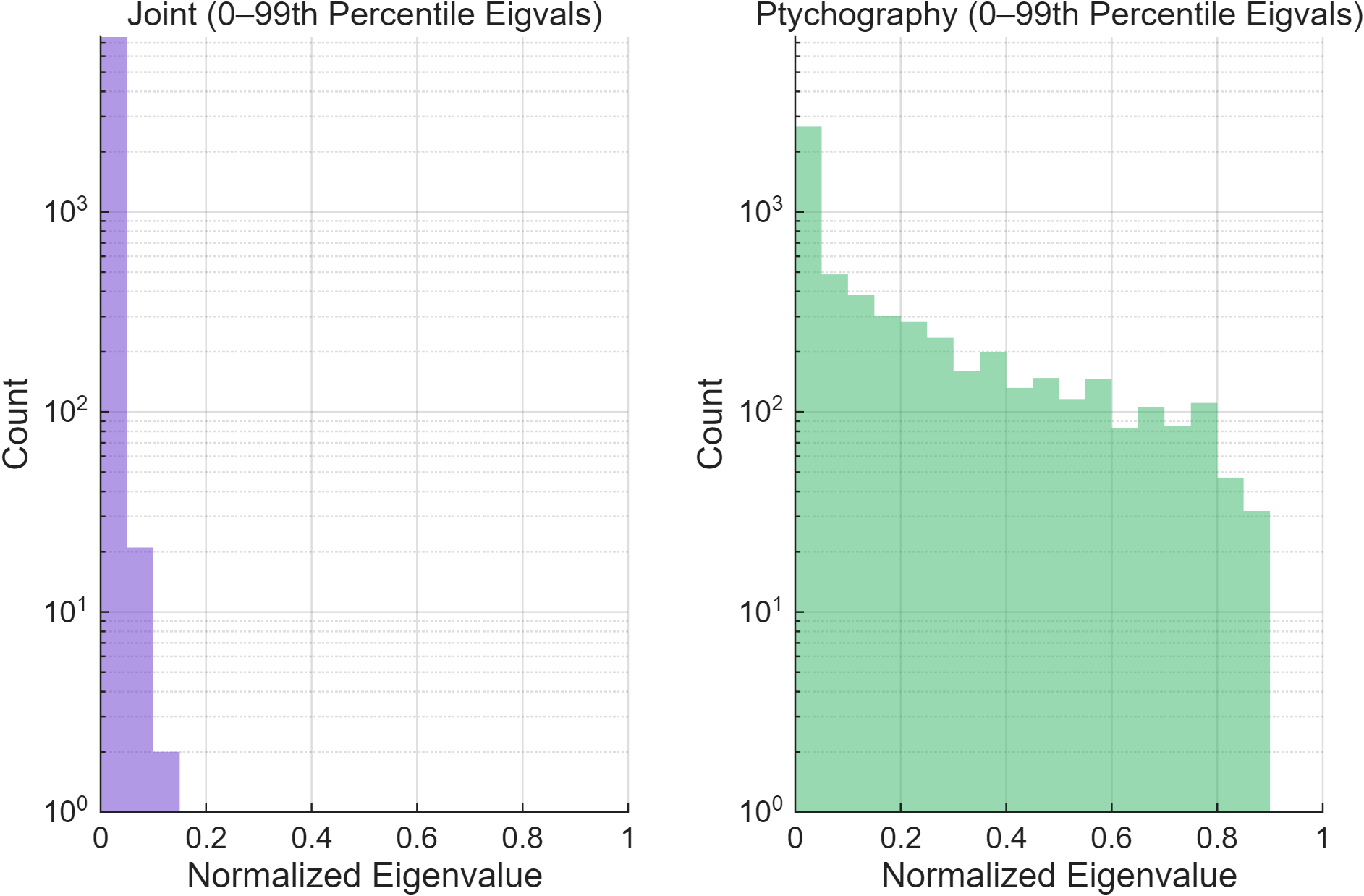
This block structure makes explicit that the fluorescence term adds positive curvature to the ptychography Hessian. To quantify how this changes optimization, we analyze the eigenvalue distribution of the joint Hessian under a deliberately challenging synthetic setup: object size $62\times 62$, one element map ($N_{e}=1$), probe size $16\times 16$, $6.25\%$ overlap, noiseless data, and a Hessian of size $7688\times 7688$. The very low overlap makes the baseline (ptychography-only) problem highly ill-conditioned. Because the Hessian spectrum encodes local curvature of the loss, it offers direct insight into optimization behavior [15]. For shape comparison, we normalize eigenvalues by the maximum, $\tilde{\lambda}_{i}=\lambda_{i}/\lambda_{\max}(H)$.

Figure 2 shows that the ptychography-only Hessian has a relatively even distribution of eigenvalues across $[0,1]$, reflecting many weakly curved directions. By contrast, the joint Hessian exhibits a two-phase spectrum: the bulk ($\approx 99\%$) is tightly clustered near zero, while a small fraction ($\approx 1\%$) form outliers at much larger values, generating a clear spectral gap. This structure indicates that the joint objective has stronger curvature along a few informative directions, enhancing local identifiability and improving the effectiveness of descent updates within these subspaces [23].

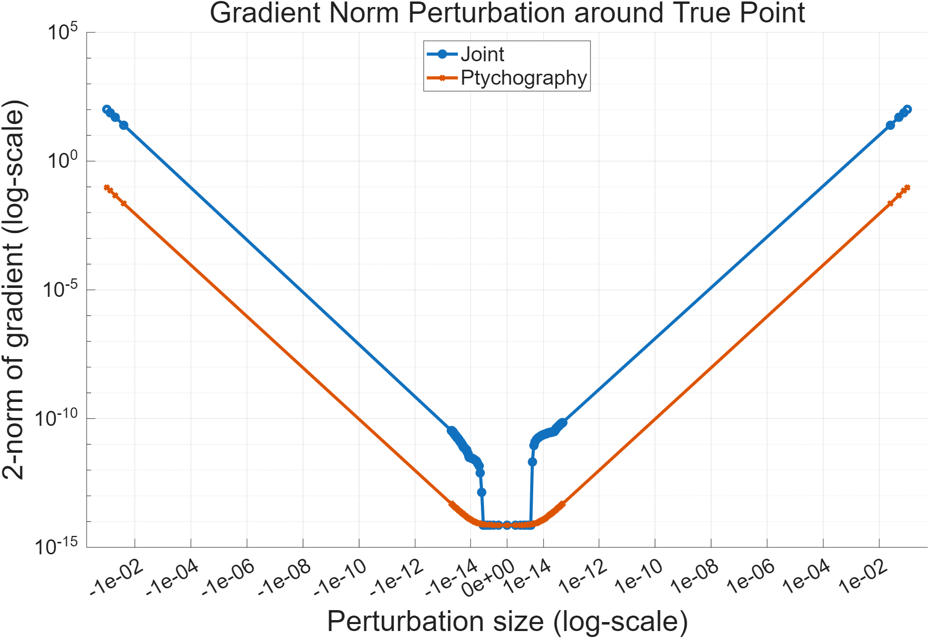
A complementary gradient–perturbation experiment around the ground truth (Figure 3) reinforces this interpretation. For perturbations $\Delta$ taken along the eigenvector corresponding to the largest eigenvalue, we vary the perturbation magnitude $|\Delta|$ continuously up to $0.1$ in both positive and negative directions. In this neighborhood, the local linearization $\nabla\Phi(z^{\star}+\Delta)\approx H\Delta$ holds for a loss function $\Phi$ evaluated near the global optimum $z^{\star}$. The faster growth of $|\nabla\Phi^{\text{joint}}(z^{\star}+\Delta)|$ relative to $|\nabla\Phi^{\text{ptyc}}(z^{\star}+\Delta)|$ within the $10^{-14}$ perturbation range reflects the larger eigenvalues in the informative subspace of $H^{\text{joint}}$. In this regime, stronger curvature tightens the link between loss reduction and reconstruction error.

Figure 2: Normalized eigenvalue distribution comparison in reconstruction.

Figure 3: True point gradient norm perturbation log-scale plot with illustration.

3.3 Evolving structure of the Hessian

Having analyzed the joint Hessian’s spectrum at a fixed point, we now ask whether the joint formulation activates more informative curvature directions throughout optimization. While the spectrum remains dominated by a small set of outliers, the joint model also lifts additional modes above a fixed tolerance. To quantify this effect, we track the numerical rank

$$r_{\tau}(H):=\#\{\sigma_{i}(H)\geq\tau\},\qquad\tau=10^{-4},$$

for both the ptychography Hessian in Eq. (3) and the joint Hessian in Eq. (4) at several iterations.

Table 1 reports the results. Across all iterations, $r_{\tau}(H^{\text{joint}})$ consistently exceeds $r_{\tau}(H^{\text{ptyc}})$. The relative gain is modest ($\approx 2.6$–$4.3\%$) in early iterations but grows to $10.1$–$10.7\%$ at later stages.

In high-dimensional models, numerical rank serves as a proxy for the dimensionality of informative curvature [1]. A low rank indicates redundancy, with many parameters contributing little to curvature, whereas a higher rank means more directions are independently active. From this perspective, the joint Hessian not only produces strong outliers (anchoring the landscape with sharp curvature in a few highly informative directions) but also broadens the subspace above the noise floor by engaging additional modes. Thus, the fluorescence term contributes in two complementary ways: it sharpens critical features through large eigenvalues, and it expands the set of active directions through rank gains. Together, these effects reduce redundancy and make optimization more stable and effective.

Iteration	$r_{\tau}(H^{\text{ptyc}})$	$r_{\tau}(H^{\text{joint}})$	$\Delta$	%$\uparrow$
$25$	$7201$	$7390$	$+189$	$+2.6\%$
$50$	$6867$	$7163$	$+296$	$+4.3\%$
$150$	$6045$	$6656$	$+611$	$+10.1\%$
$250$	$5982$	$6619$	$+637$	$+10.6\%$
$375$	$5972$	$6622$	$+650$	$+10.9\%$
$500$	5978	6621	+643	+10.7%

Table 1: Numerical rank $r_{\tau}(H)$ with $\tau=10^{-4}$ (number of singular values $\geq\tau$). The joint Hessian consistently achieves a higher rank, indicating more active optimization directions.

3.4 Sharpness and smoothness

Building on the outlier–bulk spectrum and rank growth observed in the previous subsections, we next probe the geometry of the loss surface through two-dimensional slices. As shown in [14], highly irregular landscapes can impede optimization.

We visualize the loss around the current reconstruction $\theta^{\star}$ by perturbing along two orthonormal directions $v_{1},v_{2}$:

$$f(\alpha,\beta)\;=\;\Phi\!\bigl(\theta^{\star}+\alpha v_{1}+\beta v_{2}\bigr),$$

with $v_{1},v_{2}$ normalized following the filter-wise strategy of [14]. To contrast sharp versus flat subspaces, we choose $v_{1},v_{2}$ from Hessian eigenvectors: for sharp directions, the eigenvectors corresponding to the $200$th and $201$st largest eigenvalues; for flat directions, those associated with the $4000$th and $4001$st eigenvalues. For comparability, we fix the normalized perturbation range $(\alpha,\beta)\in[-5,5]^{2}$ and plot normalized values $f(\alpha,\beta)/f_{\max}$ with $f_{\max}=\max_{(\alpha,\beta)}f(\alpha,\beta)$.

The results (Figs. 4, 5) show that the joint formulation produces a markedly sharper local basin along the leading-eigenvector plane, while also yielding a smoother, more convex-like landscape along flatter directions. This combination is advantageous: strong curvature in a small informative subspace anchors critical features, while a broader set of directions with non-negligible curvature reduces redundancy and enables progress in regions that are otherwise nearly flat. Together, these effects shape a loss surface that is both globally easier to traverse and locally more decisive, resulting in improved stability and convergence.

Figure 4: Loss surface around $\theta^{\star}$ along two sharp directions (eigenvectors for the $200$th and $201$st largest eigenvalues). Comparison between ptychography (left) and joint (right). The joint landscape exhibits a steeper, more decisive basin.

Figure 5: Loss surface around $\theta^{\star}$ along two flat directions (eigenvectors for the $4000$th and $4001$st largest eigenvalues). Comparison between ptychography (left) and joint (right). The joint landscape is smoother and more convex-like.

4 Numerical experiment

In this section, we systematically compare ptychographic, XRF and joint reconstruction methods under varying experimental conditions to assess the practical benefits of our proposed formulation. All reconstructions are performed using the truncated Newton method [18], a large-scale optimization algorithm that efficiently handles nonlinear problems through inexact Hessian approximations and robust line-search updates.

We evaluate performance across five settings: varying overlap ratio, noise robustness, scalability with object size, handling of multiple elemental maps, and robustness with different sample features. All code is implemented in MATLAB and executed on an AMD $\text{R}9-8945$ CPU.

Dataset

We generate synthetic ptychography and fluorescence measurements from known complex objects and elemental concentrations.

Probe and scanning setup

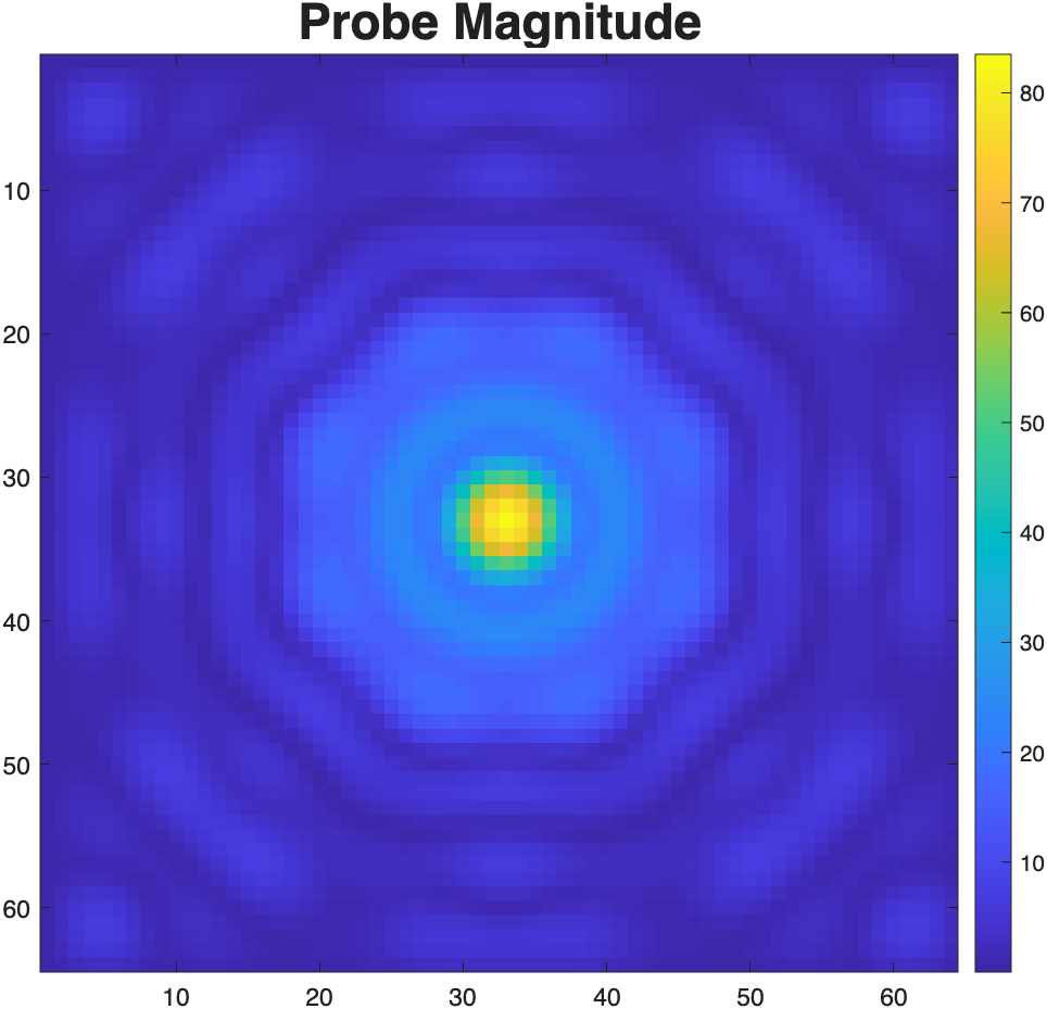
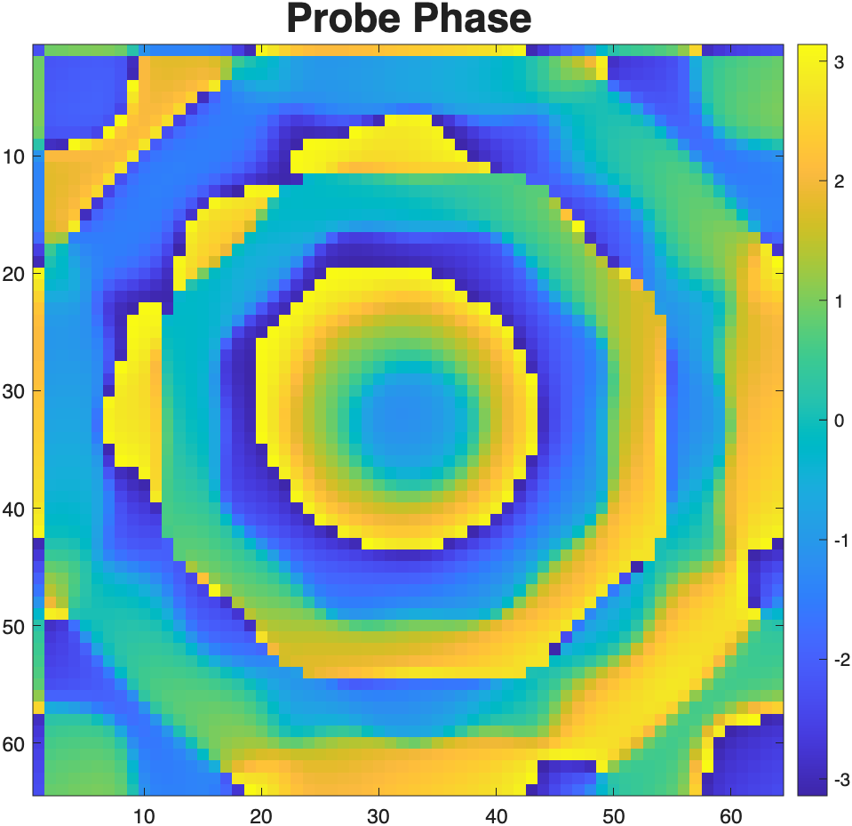
The probe is simulated as a Fresnel zone plate following [22]. Scanning positions form a regular grid with $N=64$, corresponding to a $50\%$ overlap ratio by default. Increased overlap improves identifiability and reduces ill-posedness in ptychography. Besides, as shown in the Figures 6, it is worth to notice the probe’s periphery away from the center has near-zero amplitude, which can induce ill-conditioning.

Figure 6: Magnitude (left) and phase (right) of the simulated probe matrix used in numerical experiments.

Noise model

To simulate photon-counting noise, we inject Poisson noise into both ptychographic and fluorescence measurements. Given a noiseless intensity $\hat{d}_{j}$, we define the noisy data and quantify the noise level as

$$d_{j,k}=\eta\cdot\text{Poisson}\left(\frac{\hat{d}_{j,k}}{\eta}\right),\qquad\text{Noise Level}=\sqrt{\frac{\eta}{\operatorname{mean}(\hat{d}_{j})}}\times 100\%$$

where $\eta$ is a dimensionless parameter controlling the noise level. A larger $\eta$ implies fewer photons and higher relative noise. We set $\text{Noise Level}=3\%$ by default.

Evaluation metrics

We report two complementary metrics:

• Loss: The objective value $\Phi(z)$ quantifies the consistency between the reconstruction and the measured data. For a fair comparison, we evaluate the joint model by computing the ptychographic loss function $\Phi^{\text{ptyc}}$ and fluorescence loss function $\Phi^{\text{fluor}}$ using the solution $z^{\text{joint}}$ obtained from the joint formulation (2).

• Reconstruction error: The mean squared error (MSE) between the reconstructed complex object $z$ and the ground truth $z^{*}$:

  $$\frac{1}{n^{2}}\left\|z-z^{*}\right\|_{F}^{2}.$$

This distinction is essential because in ill-posed problems, a small residual may not imply a correct solution, due to the phenomenon of semi-convergence in the presence of noise [12]. It is worth noting that the fluorescence-only reconstruction recovers only the imaginary part of the image. Therefore, for a fair comparison, we evaluate the MSE of the imaginary component of the object when comparing the fluorescence, ptychography, and joint reconstruction results.

Stopping criterion

To ensure a fair comparison, all methods and cases run for $100$ optimization steps. Final results report both loss and MSE at termination.

4.1 Effect of overlap ratio on performance

We first investigate how the overlap ratio affects reconstruction quality. We consider two representative cases: 83% overlap and 20% overlap.

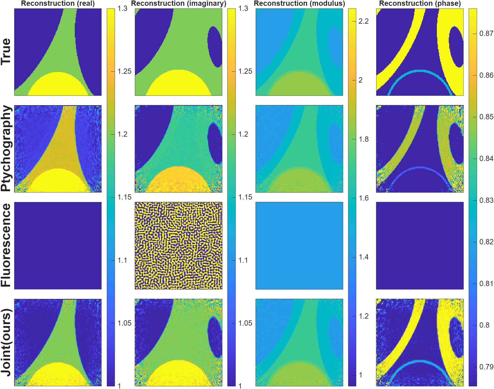
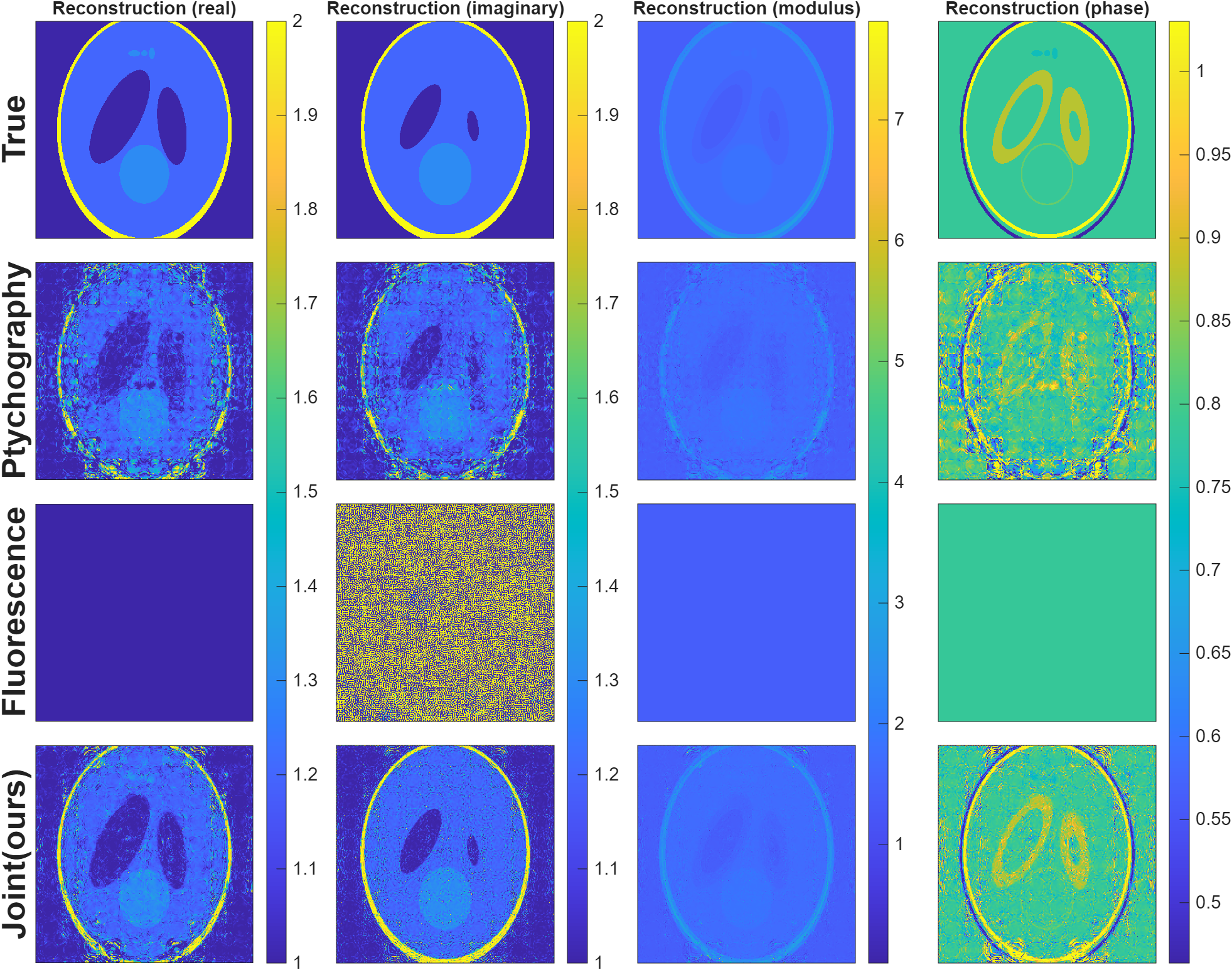
For the high-overlap case (83%), we observe a significant gap between the MSE of the ptychography reconstruction and the joint reconstruction. For the low-overlap case (20%), again, we see a major gap between the MSE for ptychography and the joint. Representative reconstructions for the true object, ptychography, fluorescence, and the joint method are shown in Figures 7 and 8. In both cases, especially in the low-overlap case, the joint approach (augmented with fluorescence data) achieves higher-quality reconstruction of both components more consistent with the true image.

By contrast, without any regularizer, the fluorescence-only method is highly sensitive to the noise due to the probe matrix’s ill-conditioning; the square-root operation further exacerbates this instability. In both cases, the fluorescence method exhibited semi-convergence to noise, yielding a blurred, noisy image after a limited number of iterations.

Figure 7: Reconstruction results for ptychography only, fluorescence only and the joint method on a synthetic object of size $n=154$ with probe size $m=64$, using $\text{Noise Level}=3\%$ and overlap ratio $0.83$. The joint method achieves more accurate reconstructions.

Figure 8: Reconstruction results for ptychography and the joint method on a larger synthetic object of size $n=514$ with probe size $m=64$, with $\text{Noise Level}=3\%$ and 20% overlap. The joint method outperforms ptychography, especially in recovering boundary details of the imaginary component.

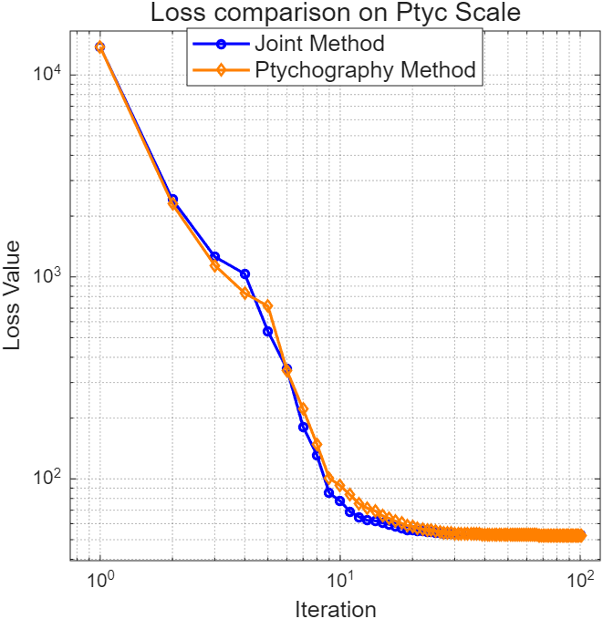
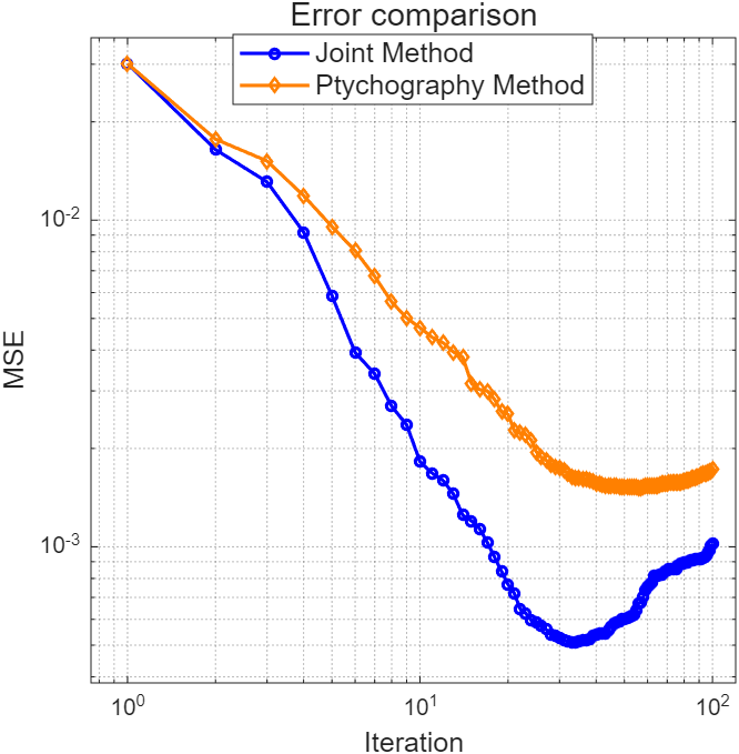
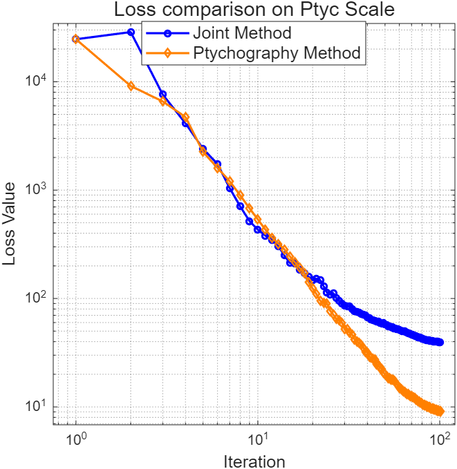
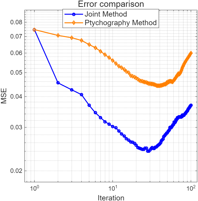
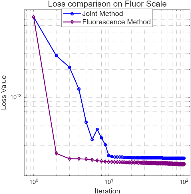
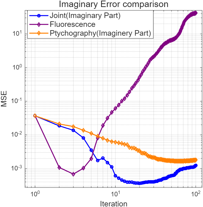
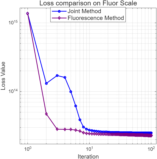
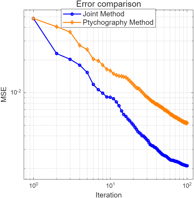
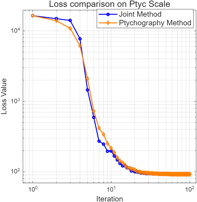
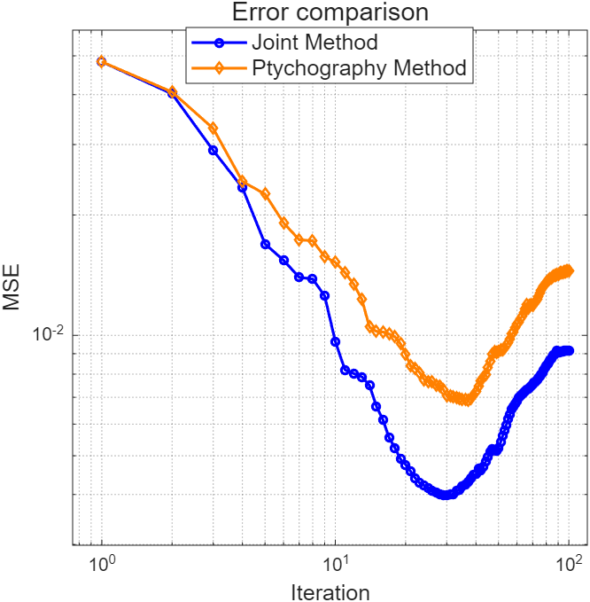
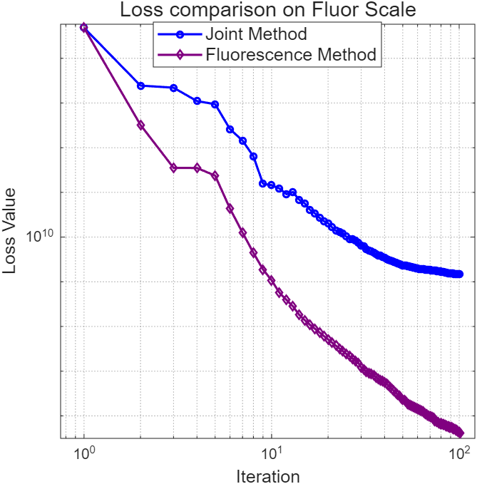
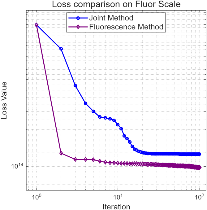
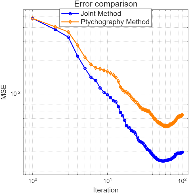
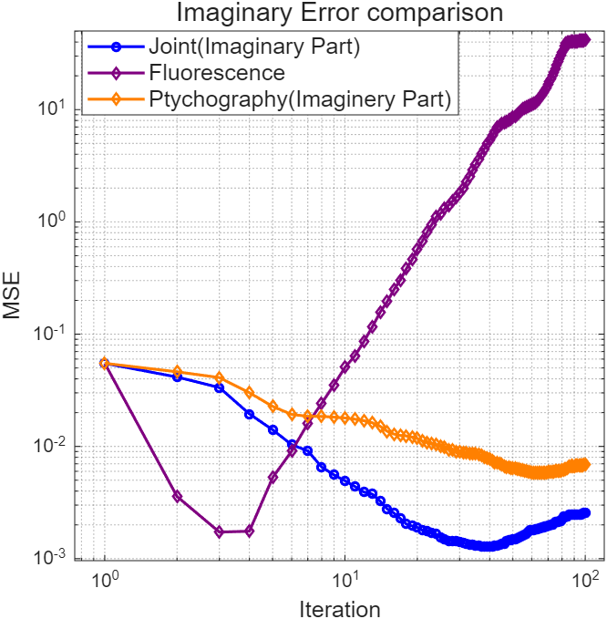
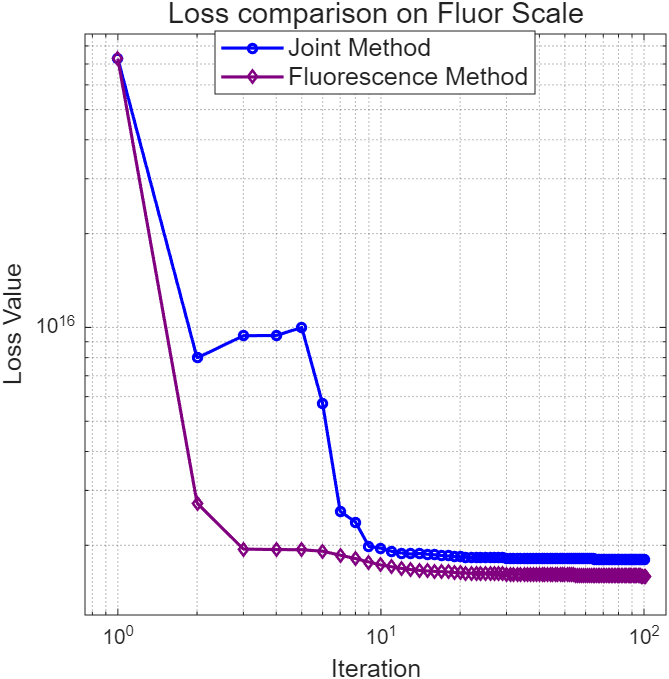
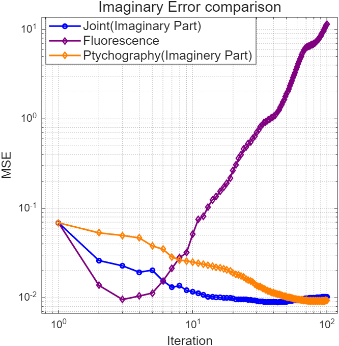
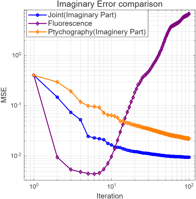
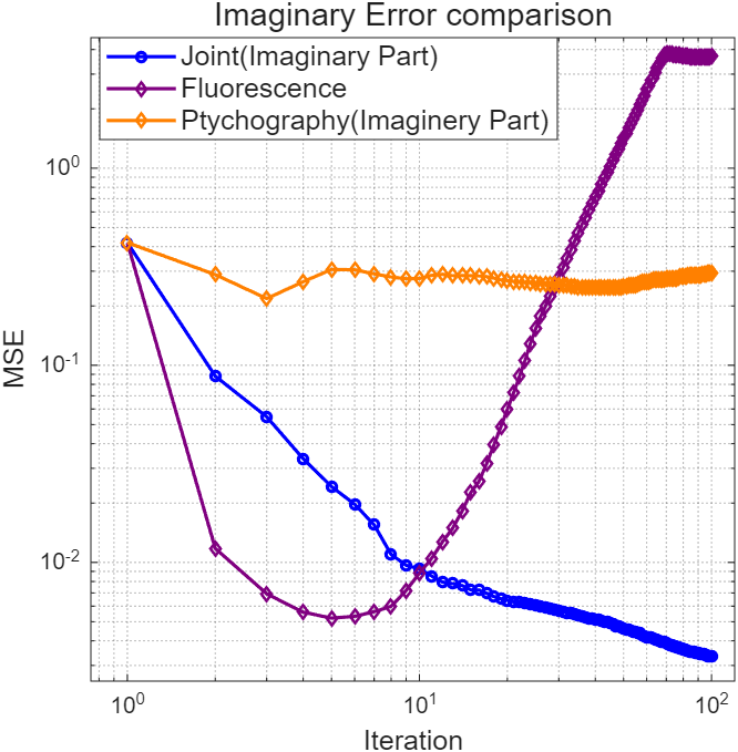
Figures 9 and 10 report the corresponding log–log plots of loss and reconstruction error. The trends confirm our earlier analysis: the joint objective introduces additional curvature in the imaginary component, broadening the effective search directions during optimization. As a result, the joint method attains substantially lower MSE at the same loss level, highlighting its robustness across overlap conditions.

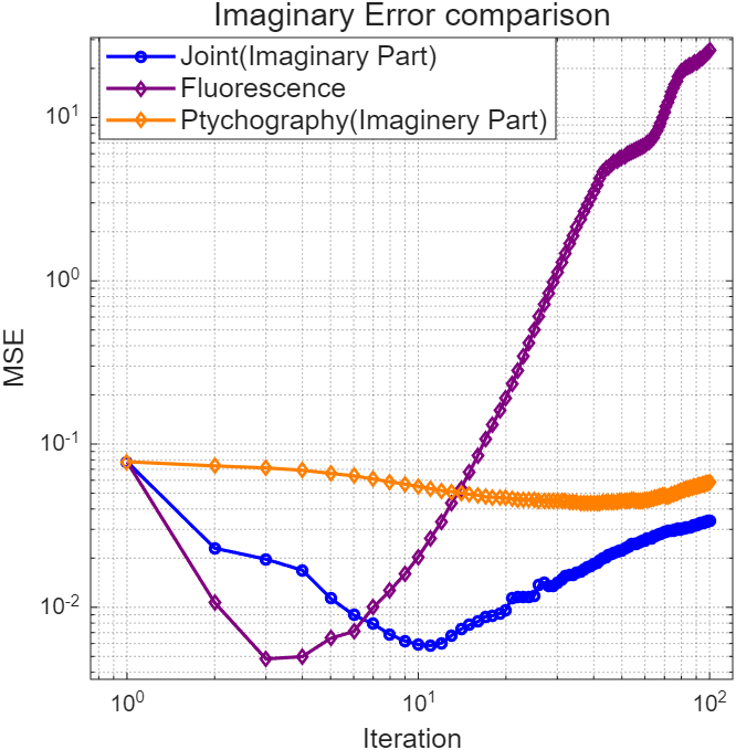
As shown in Figure 11, the fluorescence MSE only decreases for the first few iterations and then rises due to the semi-convergence effect. By incorporating constraints from the ptychography data, the joint reconstruction demonstrates improved robustness against Poisson noise while maintaining relatively lower MSE, consistent with our theoretical expectation.

Figure 9: Log–log plots of loss (left) and reconstruction error (right) for ptychography and the joint method on a synthetic object of size $n=154$ with probe size $m=64$, with $\text{Noise Level}=3\%$ and 83% overlap. The joint method converges comparatively and achieves lower error.

Figure 10: Log–log plots of loss (left) and reconstruction error (right) for ptychography and the joint method on a synthetic object of size $n=514$ with probe size $m=64$, with $\text{Noise Level}=3\%$ and 20% overlap. The joint method maintains lower error throughout optimization compared with ptychography-only method.

$n=154$, overlap $=0.83$

$n=514$, overlap $=0.2$

Figure 11: Log–log plots of objective loss (top) and reconstruction error (bottom) for fluorescence and the joint method under $\text{Noise Level}=3\%$ noise and $m=64$. Joint method exhibit stronger robustness to the input noise while maintaining lower MSE.

4.2 Stability under noise

The joint method maintains high accuracy even in the presence of noise. To evaluate stability, we compare the joint and ptychography methods across different noise levels by adding Poisson noise to the ptychography data. Two cases are considered: $\text{Noise Level}=\{0\%,10\%\}$.

Figure 12 shows reconstruction results for both settings, while Figures 13, 14 present the corresponding loss and error curves. Across both noise levels, the joint method consistently outperforms ptychography-only method. In the noise-free case, this robustness arises because the fluorescence modality provides a strong regularization effect on the imaginary part of the reconstruction, thereby preserving resolution even when the ptychography measurements are corrupted on the edges of the image. In the high-noise setting, the advantage in noise robustness becomes more pronounced. The strong regularization provided by ptychography prevents the joint reconstruction from being corrupted by the input noise, unlike the fluorescence-only reconstruction.

$\text{Noise Level}=0\%$

$\text{Noise Level}=10\%$

Figure 12: Reconstruction results for ptychography and joint method applied to a synthetic object with $n=334$, 53% overlap, and probe size $m=64$, under two noise settings.

$\text{Noise Level}=0\%$: loss (top), error (bottom)

$\text{Noise Level}=10\%$: loss (top), error (bottom)

Figure 13: Log–log plots of loss (top) and reconstruction error (bottom) for ptychography and joint method applied to a synthetic object with $n=334$, probe size $m=64$, and 53% overlap.

$\text{Noise Level}=0\%$

$\text{Noise Level}=10\%$

Figure 14: Log–log plots of loss (top) and reconstruction error (bottom) for fluorescence and joint method applied to a synthetic object with $n=334$, probe size $m=64$, and 53% overlap. The joint method has a relatively lower MSE in the high-noise setting.

4.3 Stability under varying object size

In this experiment, we investigate the effect of object size while maintaining a fixed overlap ratio. To achieve this, the step size is increased while simultaneously adjusting the number of scanning positions to preserve the overlap ratio. We consider two cases: an object of size $n=314$ with overlap ratio $0.531$, and a larger object of size $n=650$ with overlap ratio $0.5$. The corresponding reconstructions are shown in Figure 15, and the loss/error plots are reported in Figures 16, 17. Across both settings, the joint method consistently outperforms standard ptychography and achieves lower MSE with greater noise robustness than standard fluorescence.

$n=334$, $m=64$, 53% overlap

$n=650$, $m=100$, 50% overlap

Figure 15: Reconstruction results for synthetic objects of different sizes with $\text{Noise Level}=3\%$. The joint method produces sharper and more accurate reconstructions than ptychography and fluorescence alone across both object sizes.

$n=334$, $m=64$, overlap $=0.53$

$n=650$, $m=100$, overlap $=0.5$

Figure 16: Log–log plots of objective loss (top) and reconstruction error (bottom) for ptychography and the joint method under $\text{Noise Level}=3\%$ noise. The joint method exhibits faster convergence and lower error in both object-size settings.

$n=334$, $m=64$, overlap $=0.53$

$n=650$, $m=100$, overlap $=0.5$

Figure 17: Log–log plots of objective loss (top) and reconstruction error (bottom) for fluorescence and the joint method under $\text{Noise Level}=3\%$ noise. The joint method exhibits stronger robustness to noise and relatively lower MSE in both settings.

4.4 Multiple element maps

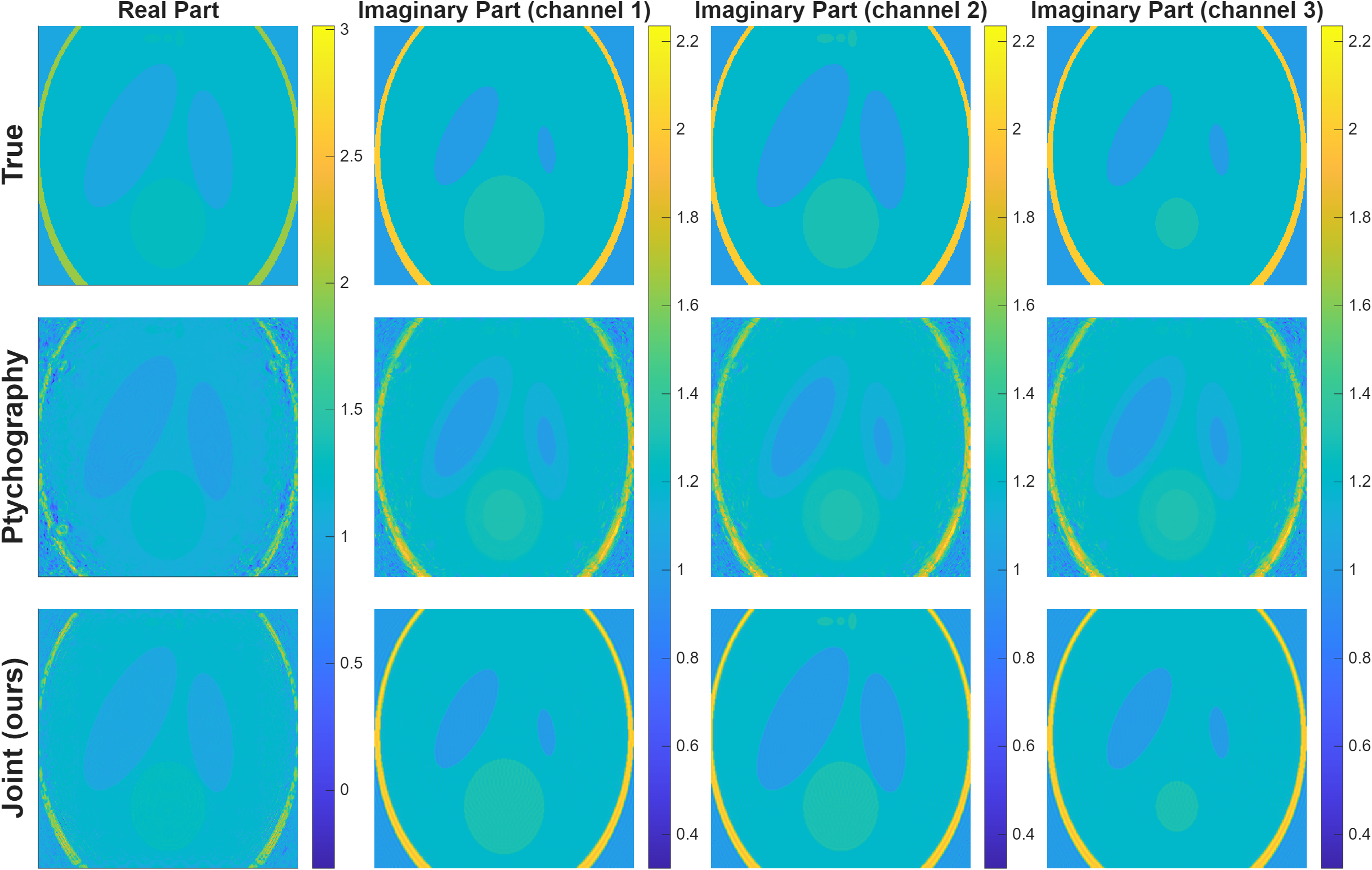
To assess the robustness of our joint framework with richer multimodal data, we extend the previous experiment by incorporating multiple elemental concentration maps into the imaginary part of both the joint and ptychography reconstructions. Specifically, we simulate $N_{e}=3$ elements, corresponding to fluorescence measurements $\{D_{e}\}_{e=1}^{3}$.

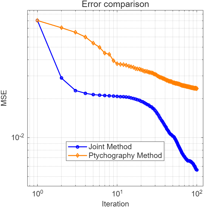
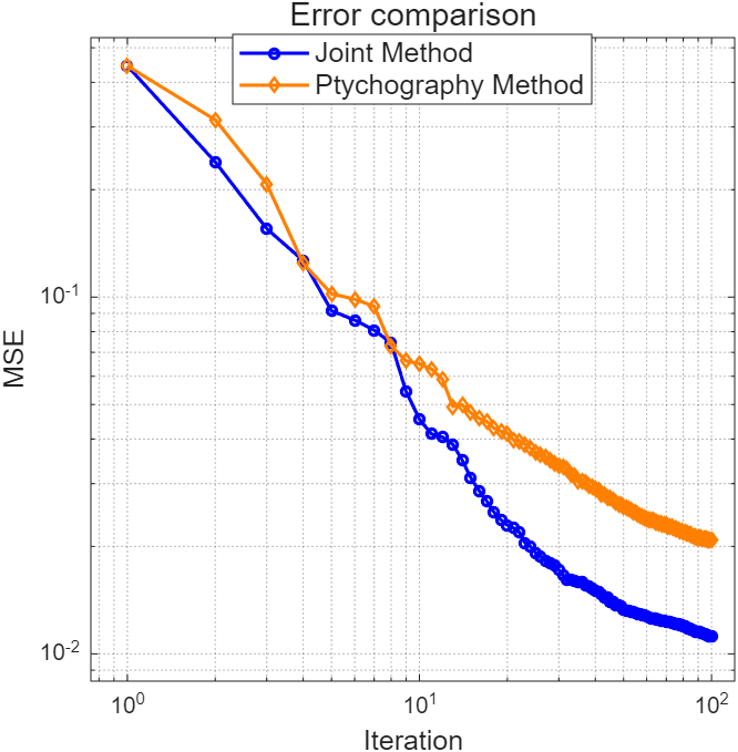
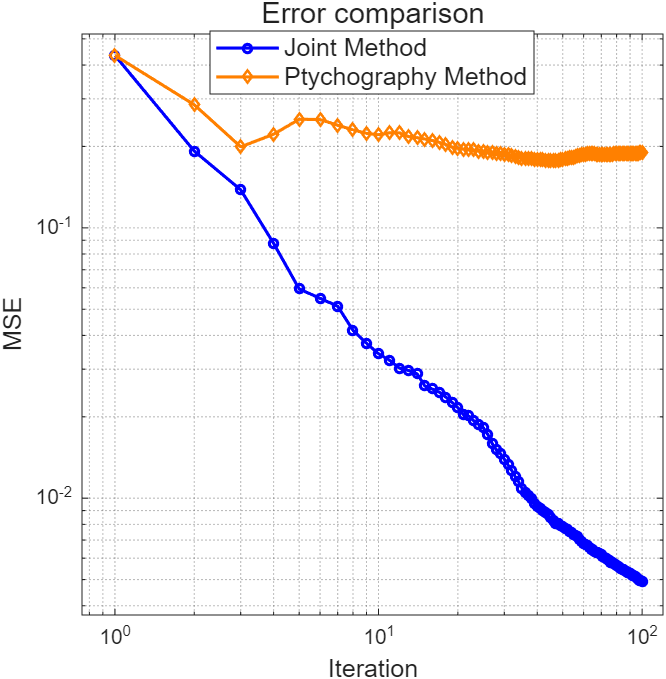
With the additional information, the joint reconstruction successfully recovers all three elemental maps with better accuracy, as shown in Figure 18. Moreover, the availability of multiple fluorescence channels strengthens the overall constraints on the reconstruction problem: even the real part of the joint reconstruction significantly outperforms ptychography, underscoring the benefit of integrating multimodal fluorescence signals as complementary information.

Figure 18: Joint and ptychography reconstructions running $200$ iterations on synthetic objects with $n=334$, overlap ratio $=0.53$, $\text{Noise Level}=0\%$, and $N_{e}=3$. Left: reconstruction images across multiple channels. Right: corresponding MSE comparison.

4.5 Robustness across different datasets

We further evaluate the robustness of the joint method on a composite dataset constructed by combining two standard test images: Cameraman (magnitude) and Baboon (phase). Both images are normalized to the range $[0,1]$, and the central $256\times 256$ region of the Baboon image is cropped to match the size of the Cameraman image. Compared with the earlier synthetic dataset, this construction introduces sharper edges and richer textures. As shown in Figures 19 and 20, the joint method yields consistently lower errors and clearer reconstructions than ptychography alone. The joint method maintains its superior robustness to input noise compared to fluorescence reconstruction alone, as shown in Figure 21. These results demonstrate that the performance advantage of the joint approach extends across diverse datasets.

$n=216$, $m=36$, 44.4% overlap

$n=244$, $m=64$, 68.5% overlap

Figure 19: Reconstruction results for the Cameraman–Baboon dataset under $\text{Noise Level}=3\%$ noise. The joint method produces sharper and more accurate reconstructions than ptychography alone across different parameter settings.

$n=216$, $m=36$, 44.4% overlap

$n=244$, $m=64$, 68.5% overlap

Figure 20: Log–log plots of objective loss (top row) and reconstruction error (bottom row) for ptychography and the joint method on the Cameraman–Baboon dataset under $\text{Noise Level}=3\%$. In both settings, the joint method converges faster and attains lower error.

$n=216$, $m=36$, 44.4% overlap

$n=244$, $m=64$, 68.5% overlap

Figure 21: Log–log plots of objective loss (top row) and reconstruction error (bottom row) for fluorescence and the joint method on the Cameraman–Baboon dataset under $\text{Noise Level}=3\%$.

5 Conclusion

In this work, we present a joint reconstruction framework that integrates ptychography and X-ray fluorescence to enable more robust and quantitative recovery of the object. By combining complementary modalities, the proposed approach mitigates the intrinsic limitations of each method, addressing the resolution constraints of fluorescence imaging and the data incompleteness challenges of ptychography. Numerical experiments demonstrate substantial improvements over single-modality reconstructions, particularly in mean-squared error, highlighting the advantages of exploiting complementary physical information within a unified optimization framework.

Several limitations remain. In all experiments, the probe function was fixed at its true position, reducing the fluorescence loss [Eq. 1] to a linear form; incorporating blind probe updates would make the model more realistic and applicable to experimental data. The current linear link function provides only a first-order approximation of the relationship between elemental concentrations and attenuation; more expressive nonlinear or learned mappings [26] may improve quantitative accuracy.

References

- [1] Ilona Ambartsumyan, Wajih Boukaram, Tan Bui-Thanh, Omar Ghattas, David Keyes, Georg Stadler, George Turkiyyah, and Stefano Zampini. Hierarchical matrix approximations of hessians arising in inverse problems governed by pdes, 2020.
- [2] Burkhard Beckhoff, Birgit Kanngießer, Norbert Langhoff, Reiner Wedell, and Helmut Wolff. Handbook of practical X-ray fluorescence analysis. Springer Science & Business Media, 2007.
- [3] Kevin Bui and Zichao Wendy Di. A stochastic admm algorithm for large-scale ptychography with weighted difference of anisotropic and isotropic total variation. Inverse Problems, 40(5):055006, 2024.
- [4] Huibin Chang, Pablo Enfedaque, and Stefano Marchesini. Blind ptychographic phase retrieval via convergent alternating direction method of multipliers. SIAM Journal on Imaging Sciences, 12(1):153–185, 2019.
- [5] Huibin Chang, Roland Glowinski, Stefano Marchesini, Xue cheng Tai, Yang Wang, and Tieyong Zeng. Overlapping domain decomposition methods for ptychographic imaging, 2021.
- [6] Zhao Chen, Vijay Badrinarayanan, Chen-Yu Lee, and Andrew Rabinovich. Gradnorm: Gradient normalization for adaptive loss balancing in deep multitask networks. CoRR, abs/1711.02257, 2017.
- [7] Junjing Deng, David J. Vine, Si Chen, Qiaoling Jin, Youssef S.G̃. Nashed, Tom Peterka, Stefan Vogt, and Chris Jacobsen. X-ray ptychographic and fluorescence microscopy of frozen-hydrated cells using continuous scanning. Scientific Reports, 7(1):445, March 2017.
- [8] Zichao Di, Sven Leyffer, and Stefan M Wild. Optimization-based approach for joint x-ray fluorescence and transmission tomographic inversion. SIAM Journal on Imaging Sciences, 9(1):1–23, 2016.
- [9] Zichao Wendy Di, Si Chen, Young Pyo Hong, Chris Jacobsen, Sven Leyffer, and Stefan M. Wild. Joint reconstruction of x-ray fluorescence and transmission tomography. Opt. Express, 25(12):13107–13124, Jun 2017.
- [10] Veit Elser. Phase retrieval by iterated projections. Journal of the Optical Society of America A, 20(1):40–55, 2003.
- [11] Samy Wu Fung and Zichao Wendy Di. Multigrid optimization for large-scale ptychographic phase retrieval. SIAM Journal on Imaging Sciences, 13(1):214–233, 2020.
- [12] Per Christian Hansen. Discrete Inverse Problems: Insight and Algorithms. Society for Industrial and Applied Mathematics, USA, 2010.
- [13] Robert Hesse, D Russell Luke, Shoham Sabach, and Matthew K Tam. Proximal heterogeneous block implicit-explicit method and application to blind ptychographic diffraction imaging. SIAM Journal on Imaging Sciences, 8(1):426–457, 2015.
- [14] Hao Li, Zheng Xu, Gavin Taylor, Christoph Studer, and Tom Goldstein. Visualizing the loss landscape of neural nets, 2018.
- [15] Zhenyu Liao and Michael W. Mahoney. Hessian eigenspectra of more realistic nonlinear models, 2021.
- [16] Andrew Maiden, Daniel Johnson, and Peng Li. Further improvements to the ptychographical iterative engine. Optica, 4(7):736–745, 2017.
- [17] Andrew M. Maiden, Martin J. Humphry, Fucai Zhang, and John M. Rodenburg. Superresolution imaging via ptychography. J. Opt. Soc. Am. A, 28(4):604–612, Apr 2011.
- [18] Stephen G Nash. A survey of truncated-Newton methods. Journal of computational and applied mathematics, 124(1-2):45–59, 2000.
- [19] Michal Odstrčil, Andreas Menzel, and Manuel Guizar-Sicairos. Iterative least-squares solver for generalized maximum-likelihood ptychography. Optics express, 26(3):3108–3123, 2018.
- [20] Franz Pfeiffer. X-ray ptychography. Nature Photonics, 12(1):9–17, 2018.
- [21] John M Rodenburg and Helen ML Faulkner. A phase retrieval algorithm for shifting illumination. Applied physics letters, 85(20):4795–4797, 2004.
- [22] John Marius Rodenburg. Ptychography and related diffractive imaging methods. Advances in Imaging and Electron Physics, 150:87–184, 2008.
- [23] Levent Sagun, Leon Bottou, and Yann LeCun. Eigenvalues of the hessian in deep learning: Singularity and beyond, 2017.
- [24] Jonathan Schwartz, Zichao Wendy Di, Yi Jiang, Alyssa J Fielitz, Don-Hyung Ha, Sanjaya D Perera, Ismail El Baggari, Richard D Robinson, Jeffrey A Fessler, Colin Ophus, et al. Imaging atomic-scale chemistry from fused multi-modal electron microscopy. npj Computational Materials, 8(1):16, 2022.
- [25] Jonathan Schwartz, Zichao Wendy Di, Yi Jiang, Jason Manassa, Jacob Pietryga, Yiwen Qian, Min Gee Cho, Jonathan L Rowell, Huihuo Zheng, Richard D Robinson, et al. Imaging 3d chemistry at 1 nm resolution with fused multi-modal electron tomography. Nature Communications, 15(1):3555, 2024.
- [26] Jacob Seifert, Yifeng Shao, and Allard P. Mosk. Noise-robust latent vector reconstruction in ptychography using deep generative models. Opt. Express, 32(1):1020–1033, Jan 2024.
- [27] Tianxiao Sun, Gang Sun, Fuda Yu, Yongzhi Mao, Renzhong Tai, Xiangzhi Zhang, Guangjie Shao, Zhenbo Wang, Jian Wang, and Jigang Zhou. Soft x-ray ptychography chemical imaging of degradation in a composite surface-reconstructed li-rich cathode. ACS nano, 15(1):1475–1485, 2020.
- [28] David J Vine, Daniele Pelliccia, Christian Holzner, Stephen B Baines, Andrew Berry, Ian McNulty, Stefan Vogt, Andrew G Peele, and Keith A Nugent. Simultaneous x-ray fluorescence and ptychographic microscopy of cyclotella meneghiniana. Optics Express, 20(16):18287–18296, 2012.
- [29] Liqi Zhou, Jingdong Song, Judy S Kim, Xudong Pei, Chen Huang, Mark Boyce, Luiza Mendonça, Daniel Clare, Alistair Siebert, Christopher S Allen, et al. Low-dose phase retrieval of biological specimens using cryo-electron ptychography. Nature communications, 11(1):2773, 2020.