Topological QBits in Flux-Quantized Super-Gravity

Abstract

We first give a brief exposition of our recent realization of anyonic quantum states on single M5-brane probes in 11D super-gravity backgrounds, by non-perturbative quantization of the topological sector of the self-dual tensor field on the 6D worldvolume, after its proper flux-quantization. This opens the prospect of holographic models for topological qbits away from the usual but unrealistic limit of large numbers of branes.

At the same time, the elementary homotopy-theoretic nature of the construction yields a slick expression of topological quantum gates in homotopically-typed programming languages, opening the prospect of topological-hardware aware quantum programming.

In view of these results, we end with some more meta-physical remarks on (cohesive) homotopy (type) theory in view of emergent fundamental physics and, possibly, M-theory.

 

∗	Mathematics, Division of Science; and
	Center for Quantum and Topological Systems,
	NYUAD Research Institute,
	New York University Abu Dhabi, UAE.

^†The Courant Institute for Mathematical Sciences, NYU, NY.

The authors acknowledge the support by Tamkeen under the NYU Abu Dhabi Research Institute grant CG008.

An open problem. While the hopes associated with quantum computation [30] are hard to overstate, it is a public secret that fundamental new methods are needed for realizing useful quantum computers at scale. Plausibly, these methods will inevitably need to involve topological stabilization, notably via anyonic quantum states (e.g. [80][58], i.e., via solitons whose states pick up purely topological quantum phases when moved around each other).

At the same time, despite the resulting attention that the idea of topological quantum computation [67][46] (see [66] for a survey) has thus received, the microscopic understanding of anyonic topological order has arguably remained sketchy, due to the general lack of first-principles understanding of strongly-coupled/correlated quantum systems – which may also explain the dearth of experimental realizations of topological q-bits to date: Better fundamental theory may be needed to understand how anyonic quantum states can actually arise in quantum materials.

1 Quantum gravity…

M-branes. Remarkably, a potential solution — to this host of theoretical problems arguably impeding practical progress — has emerged from the study of quantum gravity (e.g. [77]). In its locally super-symmetric enhancement, super-gravity (SuGra) shows hints of having a completion to a general theory of strongly-coupled interactions, where the dynamics of strongly-correlated quantum systems may usefully be mapped onto the fluctuations of membranes ([8, §2], whence the working title: “M-theory” [7][8]) and higher dimensional 5-branes [8, §3][25][26] inside an auxiliary higher dimensional spacetime (11D SuGra [8, §1][24]), a phenomenon famous as holographic duality [79].

For example, the phase transitions of quantum-critical superconductors, not amenable to traditional weak-coupling (“perturbative”) analysis, have been understood at least qualitatively by these gravitational M-theoretic methods [33][21][22][31][6] (review in [50][79][48][32]). More precise quantitative results cannot be expected without an actual formulation of M-theory/holography beyond the usual but unrealistic large-$N$ limit of a macroscopic number of coincident such branes.

Progress on developing M-theory any further had stagnated, but we may notice that a fundamental non-perturbative phenomenon already in classical super-gravity has received little to no attention in this context, namely the issue of “flux-quantization”. We find this to be crucial:

Flux-quantization. While the non-perturbative quantization of gravity famously remains a fundamental open problem of theoretical physics, we may observe that the higher (categorical symmetry) gauge fields that appear in the graviton super-multiplet call for a non-perturbative completion already at the classical level, namely by a flux-quantization law [65] which determines the topologically stabilized solitonic field configurations. This is classical for ordinary electromagnetism (where Dirac charge quantization in ordinary cohomology stabilizes the Abrikosov vortices observed in type II super-conductors, cf. [65, §2.1]) and it is famous for the RR-field in 10D supergravity (which a popular conjecture sees flux-quantized in topological K-cohomology, stabilizing certain non-supersymmetric D-branes, cf. [65, §4.1]), but it had received little attention for the C-field in the pivotal case of 11D SuGra (where flux-quantization will stabilize non-supersymmetric M-branes and solitons on M5-brane worldvolumes, cf. [65, §4.2]).

Non-abelian cohomology. In fact, due to the non-linear electric Gauss law,

$$\mathrm{d}\,G_{7}\;=\;\tfrac{1}{2}G_{4}\,G_{4}\,,\;\;\;\;\mbox{where\; $\mathrm{d}\,G_{4}\;=\;0\,,\;\;\;\;G_{7}\;=\;\star G_{4}$}$$ (1)

on the flux densities sourced by M-branes in 11D super-gravity (cf. [43, §3.1.3][24, Thm. 3.1]), none of the familiar Whitehead-generalized cohomology theories may serve here as flux-quantization laws (since they are intrinsically linear, or: abelian); what is needed are instead [65, §3] generalized non-abelian cohomology theories ([19, §2], generalizing the ordinary non-abelian cohomology of Chern-Weil theory which classifies gauge and gravitational instantons) that are receiving attention only more recently (such as in the study of non-abelian Poincaré duality [42]).

Classifying spaces and characters. The idea behind this powerful concept of non-abelian cohomology becomes quite simple once one realizes that all reasonable cohomology theories have and are characterized by classifying spaces $\mathcal{A}$ (cf. [65, p. 19]), so that the cohomology classes on a given space $X$ are just the homotopy classes of maps from $X$ to $\mathcal{A}$, denoted

$$H^{1}(X;\,\Omega\mathcal{A})\;=\;\mathrm{Maps}(X,\,\mathcal{A})_{\!/\mathrm{hmtpy}}\,.$$ (2)

A simple but profound rule (cf. [65, Prop. 3.7], using the fundamental theorem of dg-algebraic rational homotopy theory, cf. [19, §5]) determines the admissible flux quantization laws $H^{1}(-;\Omega\mathcal{A})$ for given flux densities $(F^{i})_{i\in I}$ satisfying Bianchi identities $\mathrm{d}F^{i}\,=\,P^{i}\big{(}\vec{F}\big{)}$: The flux species $F^{i}$ of degree $\mathrm{deg}_{i}$ must span the real $\mathrm{deg}_{i}$-homotopy groups of the classifying space $\mathcal{A}$, and the cohomology of the Bianchi identities on the free graded algebra generated by the flux densities must coincide with the real cohomology of $\mathcal{A}$.

For example (see also [65, p. 21]), vacuum electromagnetism with $\mathrm{d}\,F_{2}\,=\,0$ requires a classifying space whose real-homotopy and real-cohomology both are generated by a single element in degree 2, such as the universal first Chern class on infinite-projective space $\mathcal{A}\,\equiv\,\mathbb{C}P^{\infty}\,\simeq\,B\mathrm{U}(1)$ which classifies the ordinary 2-cohomology known from Dirac charge quantization; while the NS B-field with $\mathrm{d}\,H_{3}\,=\,0$ may similarly be flux-quantized by the next such Eilenberg-MacLane space $\mathcal{A}\,\equiv\,B^{2}\mathrm{U}(1)$ which classifies “bundle gerbes”; and the RR-fields with $\mathrm{d}F_{2k}\,=\,H_{3}\,F_{2k-2}$ require a classifying space with such a generator in every even degree – such as $\mathrm{KU}_{0}\,\equiv\,\underset{\longrightarrow_{\mathrlap{n}}}{\lim}\,B\mathrm{U}(n)\times\mathbb{Z}$ with its higher universal Chern classes – twisted to incorporate the $H_{3}$-generator, such as the Borel-construction space $\mathrm{KU}_{0}\!\sslash\!B\mathrm{U}(1)$ that classifies 3-twisted topological K-theory (cf. [65, §4.1]):

$$\leavevmode\hbox to115.46pt{\vbox to53.78pt{\pgfpicture\makeatletter\hbox{\hskip 57.73228pt\lower-26.88832pt\hbox to0.0pt{\pgfsys@beginscope\pgfsys@invoke{ }\definecolor{pgfstrokecolor}{rgb}{0,0,0}\pgfsys@color@rgb@stroke{0}{0}{0}\pgfsys@invoke{ }\pgfsys@color@rgb@fill{0}{0}{0}\pgfsys@invoke{ }\pgfsys@setlinewidth{0.4pt}\pgfsys@invoke{ }\nullfont\pgfsys@beginscope\pgfsys@invoke{ }\pgfsys@invoke{\lxSVG@closescope }\pgfsys@endscope\hbox to0.0pt{\pgfsys@beginscope\pgfsys@invoke{ }{}{}{}{{}}\hbox{\hbox{{\pgfsys@beginscope\pgfsys@invoke{ }{\offinterlineskip{}{}{{{}}{{}}{{}}}{{{}}}{{}{}{{ {}{}}}{ {}{}} {{}{{}}}{{}{}}{}{{}{}} { }{{{{}}\pgfsys@beginscope\pgfsys@invoke{ }\pgfsys@transformcm{1.0}{0.0}{0.0}{1.0}{-57.73228pt}{-26.88832pt}\pgfsys@invoke{ }\hbox{\vbox{\halign{\pgf@matrix@init@row\pgf@matrix@step@column{\pgf@matrix@startcell#\pgf@matrix@endcell}&#\pgf@matrix@padding&&\pgf@matrix@step@column{\pgf@matrix@startcell#\pgf@matrix@endcell}&#\pgf@matrix@padding\cr\hfil\hskip 13.34445pt\hbox{{\pgfsys@beginscope\pgfsys@invoke{ }{{}}\hbox{\hbox{{\pgfsys@beginscope\pgfsys@invoke{ }{{}{}{{ {}{}}}{ {}{}} {{}{{}}}{{}{}}{}{{}{}} { }{{{{}}\pgfsys@beginscope\pgfsys@invoke{ }\pgfsys@transformcm{1.0}{0.0}{0.0}{1.0}{-9.03891pt}{0.0pt}\pgfsys@invoke{ }\hbox{{\definecolor{pgfstrokecolor}{rgb}{0,0,0}\pgfsys@color@rgb@stroke{0}{0}{0}\pgfsys@invoke{ }\pgfsys@color@rgb@fill{0}{0}{0}\pgfsys@invoke{ }\hbox{${\mathrm{KU}_{0}}$} }}\pgfsys@invoke{\lxSVG@closescope }\pgfsys@endscope}}} \pgfsys@invoke{\lxSVG@closescope }\pgfsys@endscope}}} \pgfsys@invoke{\lxSVG@closescope }\pgfsys@endscope{}}}&\hskip 13.34445pt\hfil&\hfil\hskip 56.38782pt\hbox{{\pgfsys@beginscope\pgfsys@invoke{ }{{}}\hbox{\hbox{{\pgfsys@beginscope\pgfsys@invoke{ }{{}{}{{ {}{}}}{ {}{}} {{}{{}}}{{}{}}{}{{}{}} { }{{{{}}\pgfsys@beginscope\pgfsys@invoke{ }\pgfsys@transformcm{1.0}{0.0}{0.0}{1.0}{-28.0823pt}{0.0pt}\pgfsys@invoke{ }\hbox{{\definecolor{pgfstrokecolor}{rgb}{0,0,0}\pgfsys@color@rgb@stroke{0}{0}{0}\pgfsys@invoke{ }\pgfsys@color@rgb@fill{0}{0}{0}\pgfsys@invoke{ }\hbox{${\mathrm{KU}_{0}\!\sslash\!B\mathrm{U}(1)}$} }}\pgfsys@invoke{\lxSVG@closescope }\pgfsys@endscope}}} \pgfsys@invoke{\lxSVG@closescope }\pgfsys@endscope}}} \pgfsys@invoke{\lxSVG@closescope }\pgfsys@endscope}}&\hskip 32.38785pt\hfil\cr\vskip 18.00005pt\cr\hfil\hskip 0.0pt\hbox{{\pgfsys@beginscope\pgfsys@invoke{ }\pgfsys@invoke{\lxSVG@closescope }\pgfsys@endscope}}&\hskip 0.0pt\hfil&\hfil\hskip 43.88783pt\hbox{{\pgfsys@beginscope\pgfsys@invoke{ }{{}}\hbox{\hbox{{\pgfsys@beginscope\pgfsys@invoke{ }{{}{}{{ {}{}}}{ {}{}} {{}{{}}}{{}{}}{}{{}{}} { }{{{{}}\pgfsys@beginscope\pgfsys@invoke{ }\pgfsys@transformcm{1.0}{0.0}{0.0}{1.0}{-15.58232pt}{0.0pt}\pgfsys@invoke{ }\hbox{{\definecolor{pgfstrokecolor}{rgb}{0,0,0}\pgfsys@color@rgb@stroke{0}{0}{0}\pgfsys@invoke{ }\pgfsys@color@rgb@fill{0}{0}{0}\pgfsys@invoke{ }\hbox{${B^{2}\mathrm{U}(1)}$} }}\pgfsys@invoke{\lxSVG@closescope }\pgfsys@endscope}}} \pgfsys@invoke{\lxSVG@closescope }\pgfsys@endscope}}} \pgfsys@invoke{\lxSVG@closescope }\pgfsys@endscope}}&\hskip 19.88786pt\hfil\cr}}}\pgfsys@invoke{\lxSVG@closescope }\pgfsys@endscope}}}{{{{}}}{{}}{{}}{{}}}} \pgfsys@invoke{\lxSVG@closescope }\pgfsys@endscope}}} { {}{}{}}{}{ {}{}{}} {{{{{}}{ {}{}}{}{}{{}{}}}}}{}{{{{{}}{ {}{}}{}{}{{}{}}}}}{{}}{}{}{}\pgfsys@beginscope\pgfsys@invoke{ }\pgfsys@setlinewidth{0.39998pt}\pgfsys@invoke{ }{}{{ {\pgfsys@beginscope \pgfsys@setdash{}{0.0pt}\pgfsys@roundcap\pgfsys@roundjoin{} {}{}{} {}{}{} \pgfsys@moveto{-2.07988pt}{2.39986pt}\pgfsys@curveto{-1.69989pt}{0.95992pt}{-0.85313pt}{0.27998pt}{0.0pt}{0.0pt}\pgfsys@curveto{-0.85313pt}{-0.27998pt}{-1.69989pt}{-0.95992pt}{-2.07988pt}{-2.39986pt}\pgfsys@stroke\pgfsys@endscope}} }{}{}{{}}{}{}{{}}\pgfsys@moveto{-30.84338pt}{12.06891pt}\pgfsys@lineto{-7.64337pt}{12.06891pt}\pgfsys@stroke\pgfsys@invoke{ }{{}{{}}{}{}{{}}{{{}}}}{{}{{}}{}{}{{}}{{{}}{{{}}{\pgfsys@beginscope\pgfsys@invoke{ }\pgfsys@transformcm{1.0}{0.0}{0.0}{1.0}{-7.44339pt}{12.06891pt}\pgfsys@invoke{ }\pgfsys@invoke{ \lxSVG@closescope }\pgfsys@invoke{\lxSVG@closescope }\pgfsys@endscope}}{{}}}} \pgfsys@invoke{\lxSVG@closescope }\pgfsys@endscope{ {}{}{}}{}{ {}{}{}} {{{{{}}{ {}{}}{}{}{{}{}}}}}{}{{{{{}}{ {}{}}{}{}{{}{}}}}}{{}}{}{}{}\pgfsys@beginscope\pgfsys@invoke{ }\pgfsys@setlinewidth{0.39998pt}\pgfsys@invoke{ }{}{{ {\pgfsys@beginscope \pgfsys@setdash{}{0.0pt}\pgfsys@roundcap\pgfsys@roundjoin{} {}{}{} {}{}{} \pgfsys@moveto{-2.07997pt}{2.39995pt}\pgfsys@curveto{-1.69997pt}{0.95996pt}{-0.85316pt}{0.28pt}{0.0pt}{0.0pt}\pgfsys@curveto{-0.85316pt}{-0.28pt}{-1.69997pt}{-0.95996pt}{-2.07997pt}{-2.39995pt}\pgfsys@stroke\pgfsys@endscope}} }{}{}{}{{}}\pgfsys@moveto{25.34444pt}{3.2092pt}\pgfsys@lineto{25.34444pt}{-13.99089pt}\pgfsys@stroke\pgfsys@invoke{ }{{}{{}}{}{}{{}}{{{}}{{{}}{\pgfsys@beginscope\pgfsys@invoke{ }\pgfsys@transformcm{0.0}{-1.0}{1.0}{0.0}{25.34444pt}{-11.71094pt}\pgfsys@invoke{ }\pgfsys@invoke{ \lxSVG@closescope }\pgfsys@invoke{\lxSVG@closescope }\pgfsys@endscope}}{{}}{{{}}{\pgfsys@beginscope\pgfsys@invoke{ }\pgfsys@transformcm{0.0}{-1.0}{1.0}{0.0}{25.34444pt}{-14.19087pt}\pgfsys@invoke{ }\pgfsys@invoke{ \lxSVG@closescope }\pgfsys@invoke{\lxSVG@closescope }\pgfsys@endscope}}{{}}}} \pgfsys@invoke{\lxSVG@closescope }\pgfsys@endscope \pgfsys@invoke{\lxSVG@closescope }\pgfsys@endscope{}{}{}\hss}\pgfsys@discardpath\pgfsys@invoke{\lxSVG@closescope }\pgfsys@endscope\hss}}\lxSVG@closescope\endpgfpicture}}\qquad\leavevmode\hbox to69.14pt{\vbox to15.12pt{\pgfpicture\makeatletter\hbox{\hskip 34.57191pt\lower-9.01077pt\hbox to0.0pt{\pgfsys@beginscope\pgfsys@invoke{ }\definecolor{pgfstrokecolor}{rgb}{0,0,0}\pgfsys@color@rgb@stroke{0}{0}{0}\pgfsys@invoke{ }\pgfsys@color@rgb@fill{0}{0}{0}\pgfsys@invoke{ }\pgfsys@setlinewidth{0.4pt}\pgfsys@invoke{ }\nullfont\pgfsys@beginscope\pgfsys@invoke{ }\pgfsys@invoke{\lxSVG@closescope }\pgfsys@endscope\hbox to0.0pt{\pgfsys@beginscope\pgfsys@invoke{ } {{}}\hbox{\hbox{{\pgfsys@beginscope\pgfsys@invoke{ }{{}{}{{ {}{}}}{ {}{}} {{}{{}}}{{}{}}{}{{}{}} { }{{{{}}\pgfsys@beginscope\pgfsys@invoke{ }\pgfsys@transformcm{1.0}{0.0}{0.0}{1.0}{-30.83891pt}{-2.77777pt}\pgfsys@invoke{ }\hbox{{\definecolor{pgfstrokecolor}{rgb}{0,0,0}\pgfsys@color@rgb@stroke{0}{0}{0}\pgfsys@invoke{ }\pgfsys@color@rgb@fill{0}{0}{0}\pgfsys@invoke{ }\hbox{{\footnotesize\color[rgb]{0.05,0.25,0.65}\definecolor[named]{pgfstrokecolor}{rgb}{0.05,0.25,0.65} Chern character\;}} }}\pgfsys@invoke{\lxSVG@closescope }\pgfsys@endscope}}} \pgfsys@invoke{\lxSVG@closescope }\pgfsys@endscope}}} {{}}{}{{}}{}{ {}} {}{} {}{{}{}}{}{}{}{{}}{{}}{{}{}}{{}{}}{{{{}{}{{}} }}{{}} {}{}{} }{{{{}{}{{}} }}{{}} {{}{}{}{}} {{}{}{}{}} }{{{{}{}{{}} }}{{}} {{}{}{}{}} {{}{}{}{}} }{{{{}{}{{}} }}{{}} {{}{}{}{}} {{}{}{}{}} }{{{{}{}{{}} }}{{}} {{}{}{}{}} {{}{}{}{}} }{{{{}{}{{}} }}{{}} {{}{}{}{}} {{}{}{}{}} }{{{{}{}{{}} }}{{}} {{}{}{}{}} {{}{}{}{}} }{{{{}{}{{}} }}{{}} {{}{}{}{}} {{}{}{}{}} }{{{{}{}{{}} }}{{}} {{}{}{}{}} {{}{}{}{}} }{{{{}{}{{}} }}{{}} {{}{}{}{}} {{}{}{}{}} }{{{{}{}{{}} }}{{}} {{}{}{}{}} {{}{}{}{}} }{{{{}{}{{}} }}{{}} {}{}{} }{{{{}{}{{}} }}{{}} {{}} } {}{{ {\pgfsys@beginscope \pgfsys@setdash{}{0.0pt}\pgfsys@roundcap\pgfsys@roundjoin{} {}{}{} {}{}{} \pgfsys@moveto{-2.07999pt}{2.39998pt}\pgfsys@curveto{-1.69998pt}{0.95998pt}{-0.85318pt}{0.28pt}{0.0pt}{0.0pt}\pgfsys@curveto{-0.85318pt}{-0.28pt}{-1.69998pt}{-0.95998pt}{-2.07999pt}{-2.39998pt}\pgfsys@stroke\pgfsys@endscope}} }{}{}{{}}\pgfsys@moveto{-34.37192pt}{-6.31078pt}\pgfsys@curveto{-33.12192pt}{-6.31078pt}{-32.49692pt}{-3.81078pt}{-31.24692pt}{-3.81078pt}\pgfsys@curveto{-30.34192pt}{-3.81078pt}{-29.56194pt}{-5.03079pt}{-28.74692pt}{-6.31078pt}\pgfsys@curveto{-27.93192pt}{-7.59076pt}{-27.15192pt}{-8.81078pt}{-26.24692pt}{-8.81078pt}\pgfsys@curveto{-25.34192pt}{-8.81078pt}{-24.56194pt}{-7.59076pt}{-23.74692pt}{-6.31078pt}\pgfsys@curveto{-22.93192pt}{-5.03079pt}{-22.15192pt}{-3.81078pt}{-21.24692pt}{-3.81078pt}\pgfsys@curveto{-20.34192pt}{-3.81078pt}{-19.56194pt}{-5.03079pt}{-18.74692pt}{-6.31078pt}\pgfsys@curveto{-17.93192pt}{-7.59076pt}{-17.15192pt}{-8.81078pt}{-16.24692pt}{-8.81078pt}\pgfsys@curveto{-15.34192pt}{-8.81078pt}{-14.56194pt}{-7.59076pt}{-13.74692pt}{-6.31078pt}\pgfsys@curveto{-12.93192pt}{-5.03079pt}{-12.15192pt}{-3.81078pt}{-11.24692pt}{-3.81078pt}\pgfsys@curveto{-10.34192pt}{-3.81078pt}{-9.56194pt}{-5.03079pt}{-8.74692pt}{-6.31078pt}\pgfsys@curveto{-7.93192pt}{-7.59076pt}{-7.15192pt}{-8.81078pt}{-6.24692pt}{-8.81078pt}\pgfsys@curveto{-5.34192pt}{-8.81078pt}{-4.56194pt}{-7.59076pt}{-3.74692pt}{-6.31078pt}\pgfsys@curveto{-2.93192pt}{-5.03079pt}{-2.15192pt}{-3.81078pt}{-1.24692pt}{-3.81078pt}\pgfsys@curveto{-0.34192pt}{-3.81078pt}{0.43806pt}{-5.03079pt}{1.25308pt}{-6.31078pt}\pgfsys@curveto{2.06808pt}{-7.59076pt}{2.84808pt}{-8.81078pt}{3.75308pt}{-8.81078pt}\pgfsys@curveto{4.65808pt}{-8.81078pt}{5.43806pt}{-7.59076pt}{6.25308pt}{-6.31078pt}\pgfsys@curveto{7.06808pt}{-5.03079pt}{7.84808pt}{-3.81078pt}{8.75308pt}{-3.81078pt}\pgfsys@curveto{9.65808pt}{-3.81078pt}{10.43806pt}{-5.03079pt}{11.25308pt}{-6.31078pt}\pgfsys@curveto{12.06808pt}{-7.59076pt}{12.84808pt}{-8.81078pt}{13.75308pt}{-8.81078pt}\pgfsys@curveto{14.65808pt}{-8.81078pt}{15.43806pt}{-7.59076pt}{16.25308pt}{-6.31078pt}\pgfsys@curveto{17.06808pt}{-5.03079pt}{17.84808pt}{-3.81078pt}{18.75308pt}{-3.81078pt}\pgfsys@curveto{20.00308pt}{-3.81078pt}{20.62808pt}{-6.31078pt}{21.87808pt}{-6.31078pt}\pgfsys@lineto{33.97192pt}{-6.31078pt}\pgfsys@stroke\pgfsys@invoke{ }{{}{{}}{}{}{{}}{{{}}{{{}}{\pgfsys@beginscope\pgfsys@invoke{ }\pgfsys@transformcm{1.0}{0.0}{0.0}{1.0}{34.17192pt}{-6.31078pt}\pgfsys@invoke{ }\pgfsys@invoke{ \lxSVG@closescope }\pgfsys@invoke{\lxSVG@closescope }\pgfsys@endscope}}{{}}}} \pgfsys@invoke{\lxSVG@closescope }\pgfsys@endscope{}{}{}\hss}\pgfsys@discardpath\pgfsys@invoke{\lxSVG@closescope }\pgfsys@endscope\hss}}\lxSVG@closescope\endpgfpicture}}\qquad\begin{array}[]{ccl}\mathrm{d}\,F_{2\bullet}&=&H_{3}\,F_{2\bullet-2}\\ \\ \mathrm{d}\,H_{3}&=&0\mathrlap{\,.}\end{array} {\mathrm{KU}_{0}} {\mathrm{KU}_{0}\!\sslash\!B\mathrm{U}(1)} {B^{2}\mathrm{U}(1)} {\mathrm{KU}_{0}} {\mathrm{KU}_{0}\!\sslash\!B\mathrm{U}(1)} {B^{2}\mathrm{U}(1)}$$

The construction of such characters generalizes [19] to non-abelian cohomology theories:

M-Brane charge in Cohomotopy. Among the admissible flux-quantization laws for the C-field sourced by M-branes turns out to be the most fundamental and most ancient non-abelian cohomology theory there is, known as (unstable) “co-homotopy” (since its classifying spaces are nothing but spheres), introduced by Pontrjagin in the 1930s (and later baptized by Spanier).

Concretely, the real-homotopy groups of $S^{4}$ have a generator in degree 4 (the identity map) and in degree 7 (the quaternionic Hopf fibration $S^{7}\xrightarrow{h_{\mathbb{H}}}S^{4}$), while the real-cohomology only has a generator $G_{4}$ in degree 4. Hence $G_{4}$ must be closed while the other generator $G_{7}$ must be a coboundary for the otherwise induced cohomology class of $G_{4}\,G_{4}$. This way, the character map on 4-Cohomotopy reproduces the equation of motion (1) of the 11D SuGra C-field [52][63]:

$$S^{4}\qquad\leavevmode\hbox to42.34pt{\vbox to15.12pt{\pgfpicture\makeatletter\hbox{\hskip 21.17192pt\lower-9.01077pt\hbox to0.0pt{\pgfsys@beginscope\pgfsys@invoke{ }\definecolor{pgfstrokecolor}{rgb}{0,0,0}\pgfsys@color@rgb@stroke{0}{0}{0}\pgfsys@invoke{ }\pgfsys@color@rgb@fill{0}{0}{0}\pgfsys@invoke{ }\pgfsys@setlinewidth{0.4pt}\pgfsys@invoke{ }\nullfont\pgfsys@beginscope\pgfsys@invoke{ }\pgfsys@invoke{\lxSVG@closescope }\pgfsys@endscope\hbox to0.0pt{\pgfsys@beginscope\pgfsys@invoke{ } {{}}\hbox{\hbox{{\pgfsys@beginscope\pgfsys@invoke{ }{{}{}{{ {}{}}}{ {}{}} {{}{{}}}{{}{}}{}{{}{}} { }{{{{}}\pgfsys@beginscope\pgfsys@invoke{ }\pgfsys@transformcm{1.0}{0.0}{0.0}{1.0}{-17.43892pt}{-2.77777pt}\pgfsys@invoke{ }\hbox{{\definecolor{pgfstrokecolor}{rgb}{0,0,0}\pgfsys@color@rgb@stroke{0}{0}{0}\pgfsys@invoke{ }\pgfsys@color@rgb@fill{0}{0}{0}\pgfsys@invoke{ }\hbox{{\footnotesize\color[rgb]{0.05,0.25,0.65}\definecolor[named]{pgfstrokecolor}{rgb}{0.05,0.25,0.65} character}} }}\pgfsys@invoke{\lxSVG@closescope }\pgfsys@endscope}}} \pgfsys@invoke{\lxSVG@closescope }\pgfsys@endscope}}} {{}}{}{{}}{}{ {}} {}{} {}{{}{}}{}{}{}{{}}{{}}{{}{}}{{}{}}{{{{}{}{{}} }}{{}} {}{}{} }{{{{}{}{{}} }}{{}} {{}{}{}{}} {{}{}{}{}} }{{{{}{}{{}} }}{{}} {{}{}{}{}} {{}{}{}{}} }{{{{}{}{{}} }}{{}} {{}{}{}{}} {{}{}{}{}} }{{{{}{}{{}} }}{{}} {{}{}{}{}} {{}{}{}{}} }{{{{}{}{{}} }}{{}} {{}{}{}{}} {{}{}{}{}} }{{{{}{}{{}} }}{{}} {{}{}{}{}} {{}{}{}{}} }{{{{}{}{{}} }}{{}} {}{}{} }{{{{}{}{{}} }}{{}} {{}} } {}{}{}{}{{}}\pgfsys@moveto{-20.97192pt}{-6.31078pt}\pgfsys@curveto{-19.72192pt}{-6.31078pt}{-19.09692pt}{-3.81078pt}{-17.84692pt}{-3.81078pt}\pgfsys@curveto{-16.94193pt}{-3.81078pt}{-16.16194pt}{-5.03079pt}{-15.34692pt}{-6.31078pt}\pgfsys@curveto{-14.53192pt}{-7.59076pt}{-13.75192pt}{-8.81078pt}{-12.84692pt}{-8.81078pt}\pgfsys@curveto{-11.94193pt}{-8.81078pt}{-11.16194pt}{-7.59076pt}{-10.34692pt}{-6.31078pt}\pgfsys@curveto{-9.53192pt}{-5.03079pt}{-8.75192pt}{-3.81078pt}{-7.84692pt}{-3.81078pt}\pgfsys@curveto{-6.94193pt}{-3.81078pt}{-6.16194pt}{-5.03079pt}{-5.34692pt}{-6.31078pt}\pgfsys@curveto{-4.53192pt}{-7.59076pt}{-3.75192pt}{-8.81078pt}{-2.84692pt}{-8.81078pt}\pgfsys@curveto{-1.94193pt}{-8.81078pt}{-1.16194pt}{-7.59076pt}{-0.34692pt}{-6.31078pt}\pgfsys@curveto{0.46808pt}{-5.03079pt}{1.24808pt}{-3.81078pt}{2.15308pt}{-3.81078pt}\pgfsys@curveto{3.05807pt}{-3.81078pt}{3.83806pt}{-5.03079pt}{4.65308pt}{-6.31078pt}\pgfsys@curveto{5.46808pt}{-7.59076pt}{6.24808pt}{-8.81078pt}{7.15308pt}{-8.81078pt}\pgfsys@curveto{8.05807pt}{-8.81078pt}{8.83806pt}{-7.59076pt}{9.65308pt}{-6.31078pt}\pgfsys@curveto{10.46808pt}{-5.03079pt}{11.24808pt}{-3.81078pt}{12.15308pt}{-3.81078pt}\pgfsys@curveto{13.40308pt}{-3.81078pt}{14.02808pt}{-6.31078pt}{15.27808pt}{-6.31078pt}\pgfsys@lineto{20.57193pt}{-6.31078pt}\pgfsys@stroke\pgfsys@invoke{ }{{}{{}}{}{}{{}}{{{}}{{{}}{\pgfsys@beginscope\pgfsys@invoke{ }\pgfsys@transformcm{1.0}{0.0}{0.0}{1.0}{20.77193pt}{-6.31078pt}\pgfsys@invoke{ }\pgfsys@invoke{ \lxSVG@closescope }\pgfsys@invoke{\lxSVG@closescope }\pgfsys@endscope}}{{}}}} \pgfsys@invoke{\lxSVG@closescope }\pgfsys@endscope{}{}{}\hss}\pgfsys@discardpath\pgfsys@invoke{\lxSVG@closescope }\pgfsys@endscope\hss}}\lxSVG@closescope\endpgfpicture}}\qquad\begin{array}[]{ccl}\mathrm{d}\,G_{7}&=&\tfrac{1}{2}G_{4}\,G_{4}\\ \mathrm{d}\,G_{4}&=&0\;.\end{array}$$ (3)

Careful analysis shows that assuming (“Hypothesis H”) 11D supergravity to be globally completed by demanding the C-field flux densities to be quantized in (tangentially twisted) 4-Cohomotopy provably implies various subtle topological effects that are expected in M-theory [15][16][18][55], notably the condition that the sum of $G_{4}$ with $1/4$th of the first Pontrjagin form of the spin-connection is integral [15, Prop. 3.13].

3-Form flux on M5-Branes. Moreover, given an M5-brane $\Sigma^{1,5}\xhookrightarrow{\,\phi\,}X^{1,10}$ probing the bulk spacetime $X^{1,10}$, its worldvolume $\Sigma^{1,5}$ famously (but quite [34][25]) carries itself a non-linearly self-dual 3-flux density $H_{3}$ (sourced by string-like solitons inside the M5), satisfying the Bianchi identity

$$\mathrm{d}\,H_{3}\;=\;\phi^{\ast}G_{4}\,,$$ (4)

which, while nominally linear, inherits the non-linearity (1) of the source term $G_{4}$ on the right. An admissible non-abelian flux quantization law for the combination of (4) with (1) turns out to be (tangentially twisted) 7-Cohomotopy relative to the bulk 4-Cohomotopy (where (4) reflects the vanishing of the class of the volume form of $S^{4}$ upon pullback to $S^{7}$). This means that where the latter has as classifying space the 4-sphere, the former has as classifying space the 3-sphere fibers of the quaternionic Hopf fibration $\phi_{\mathbb{H}}$ [15, §3.7]:

$$\leavevmode\hbox{\raise 5.0pt\hbox{\set@color\resizebox{}{}{{\leavevmode\hbox{\set@color{ \leavevmode\hbox to129.28pt{\vbox to52.41pt{\pgfpicture\makeatletter\hbox{\hskip 59.01239pt\lower-26.20718pt\hbox to0.0pt{\pgfsys@beginscope\pgfsys@invoke{ }\definecolor{pgfstrokecolor}{rgb}{0,0,0}\pgfsys@color@rgb@stroke{0}{0}{0}\pgfsys@invoke{ }\pgfsys@color@rgb@fill{0}{0}{0}\pgfsys@invoke{ }\pgfsys@setlinewidth{0.4pt}\pgfsys@invoke{ }\nullfont\pgfsys@beginscope\pgfsys@invoke{ }\pgfsys@invoke{\lxSVG@closescope }\pgfsys@endscope\hbox to0.0pt{\pgfsys@beginscope\pgfsys@invoke{ }{}{}{}{{}}\hbox{\hbox{{\pgfsys@beginscope\pgfsys@invoke{ }{\offinterlineskip{}{}{{{}}{{}}{{}}{{}}{{}}{{}}{{}}}{{{}}}{{}{}{{ {}{}}}{ {}{}} {{}{{}}}{{}{}}{}{{}{}} { }{{{{}}\pgfsys@beginscope\pgfsys@invoke{ }\pgfsys@transformcm{1.0}{0.0}{0.0}{1.0}{-59.01239pt}{-26.20718pt}\pgfsys@invoke{ }\hbox{\vbox{\halign{\pgf@matrix@init@row\pgf@matrix@step@column{\pgf@matrix@startcell#\pgf@matrix@endcell}&#\pgf@matrix@padding&&\pgf@matrix@step@column{\pgf@matrix@startcell#\pgf@matrix@endcell}&#\pgf@matrix@padding\cr\hfil\hskip 9.0597pt\hbox{{\pgfsys@beginscope\pgfsys@invoke{ }{{}}\hbox{\hbox{{\pgfsys@beginscope\pgfsys@invoke{ }{{}{}{{ {}{}}}{ {}{}} {{}{{}}}{{}{}}{}{{}{}} { }{{{{}}\pgfsys@beginscope\pgfsys@invoke{ }\pgfsys@transformcm{1.0}{0.0}{0.0}{1.0}{-4.75415pt}{0.0pt}\pgfsys@invoke{ }\hbox{{\definecolor{pgfstrokecolor}{rgb}{0,0,0}\pgfsys@color@rgb@stroke{0}{0}{0}\pgfsys@invoke{ }\pgfsys@color@rgb@fill{0}{0}{0}\pgfsys@invoke{ }\hbox{${S^{3}}$} }}\pgfsys@invoke{\lxSVG@closescope }\pgfsys@endscope}}} \pgfsys@invoke{\lxSVG@closescope }\pgfsys@endscope}}} \pgfsys@invoke{\lxSVG@closescope }\pgfsys@endscope{}}}&\hskip 9.0597pt\hfil&\hfil\hskip 33.05966pt\hbox{{\pgfsys@beginscope\pgfsys@invoke{ }{{}}\hbox{\hbox{{\pgfsys@beginscope\pgfsys@invoke{ }{{}{}{{ {}{}}}{ {}{}} {{}{{}}}{{}{}}{}{{}{}} { }{{{{}}\pgfsys@beginscope\pgfsys@invoke{ }\pgfsys@transformcm{1.0}{0.0}{0.0}{1.0}{-4.75415pt}{0.0pt}\pgfsys@invoke{ }\hbox{{\definecolor{pgfstrokecolor}{rgb}{0,0,0}\pgfsys@color@rgb@stroke{0}{0}{0}\pgfsys@invoke{ }\pgfsys@color@rgb@fill{0}{0}{0}\pgfsys@invoke{ }\hbox{${S^{7}}$} }}\pgfsys@invoke{\lxSVG@closescope }\pgfsys@endscope}}} \pgfsys@invoke{\lxSVG@closescope }\pgfsys@endscope}}} \pgfsys@invoke{\lxSVG@closescope }\pgfsys@endscope{}}}&\hskip 9.0597pt\hfil&\hfil\hskip 12.19441pt\hbox{{\pgfsys@beginscope\pgfsys@invoke{ }{{}}\hbox{\hbox{{\pgfsys@beginscope\pgfsys@invoke{ }{{}{}{{ {}{}}}{ {}{}} {{}{{}}}{{}{}}{}{{}{}} { }{{{{}}\pgfsys@beginscope\pgfsys@invoke{ }\pgfsys@transformcm{1.0}{0.0}{0.0}{1.0}{-3.8889pt}{0.0pt}\pgfsys@invoke{ }\hbox{{\definecolor{pgfstrokecolor}{rgb}{0,0,0}\pgfsys@color@rgb@stroke{0}{0}{0}\pgfsys@invoke{ }\pgfsys@color@rgb@fill{0}{0}{0}\pgfsys@invoke{ }\hbox{${\simeq}$} }}\pgfsys@invoke{\lxSVG@closescope }\pgfsys@endscope}}} \pgfsys@invoke{\lxSVG@closescope }\pgfsys@endscope}}} \pgfsys@invoke{\lxSVG@closescope }\pgfsys@endscope{}}}&\hskip 8.19444pt\hfil&\hfil\hskip 20.69858pt\hbox{{\pgfsys@beginscope\pgfsys@invoke{ }{{}}\hbox{\hbox{{\pgfsys@beginscope\pgfsys@invoke{ }{{}{}{{ {}{}}}{ {}{}} {{}{{}}}{{}{}}{}{{}{}} { }{{{{}}\pgfsys@beginscope\pgfsys@invoke{ }\pgfsys@transformcm{1.0}{0.0}{0.0}{1.0}{-12.39307pt}{0.0pt}\pgfsys@invoke{ }\hbox{{\definecolor{pgfstrokecolor}{rgb}{0,0,0}\pgfsys@color@rgb@stroke{0}{0}{0}\pgfsys@invoke{ }\pgfsys@color@rgb@fill{0}{0}{0}\pgfsys@invoke{ }\hbox{${S(\mathbb{H}^{2})}$} }}\pgfsys@invoke{\lxSVG@closescope }\pgfsys@endscope}}} \pgfsys@invoke{\lxSVG@closescope }\pgfsys@endscope}}} \pgfsys@invoke{\lxSVG@closescope }\pgfsys@endscope}}&\hskip 16.69861pt\hfil\cr\vskip 18.0pt\cr\hfil\hskip 0.0pt\hbox{{\pgfsys@beginscope\pgfsys@invoke{ }\pgfsys@invoke{\lxSVG@closescope }\pgfsys@endscope}}&\hskip 0.0pt\hfil&\hfil\hskip 33.05966pt\hbox{{\pgfsys@beginscope\pgfsys@invoke{ }{{}}\hbox{\hbox{{\pgfsys@beginscope\pgfsys@invoke{ }{{}{}{{ {}{}}}{ {}{}} {{}{{}}}{{}{}}{}{{}{}} { }{{{{}}\pgfsys@beginscope\pgfsys@invoke{ }\pgfsys@transformcm{1.0}{0.0}{0.0}{1.0}{-4.75415pt}{0.0pt}\pgfsys@invoke{ }\hbox{{\definecolor{pgfstrokecolor}{rgb}{0,0,0}\pgfsys@color@rgb@stroke{0}{0}{0}\pgfsys@invoke{ }\pgfsys@color@rgb@fill{0}{0}{0}\pgfsys@invoke{ }\hbox{${S^{4}}$} }}\pgfsys@invoke{\lxSVG@closescope }\pgfsys@endscope}}} \pgfsys@invoke{\lxSVG@closescope }\pgfsys@endscope}}} \pgfsys@invoke{\lxSVG@closescope }\pgfsys@endscope}}&\hskip 9.0597pt\hfil&\hfil\hskip 12.19441pt\hbox{{\pgfsys@beginscope\pgfsys@invoke{ }{{}}\hbox{\hbox{{\pgfsys@beginscope\pgfsys@invoke{ }{{}{}{{ {}{}}}{ {}{}} {{}{{}}}{{}{}}{}{{}{}} { }{{{{}}\pgfsys@beginscope\pgfsys@invoke{ }\pgfsys@transformcm{1.0}{0.0}{0.0}{1.0}{-3.8889pt}{0.0pt}\pgfsys@invoke{ }\hbox{{\definecolor{pgfstrokecolor}{rgb}{0,0,0}\pgfsys@color@rgb@stroke{0}{0}{0}\pgfsys@invoke{ }\pgfsys@color@rgb@fill{0}{0}{0}\pgfsys@invoke{ }\hbox{${\simeq}$} }}\pgfsys@invoke{\lxSVG@closescope }\pgfsys@endscope}}} \pgfsys@invoke{\lxSVG@closescope }\pgfsys@endscope}}} \pgfsys@invoke{\lxSVG@closescope }\pgfsys@endscope}}&\hskip 8.19444pt\hfil&\hfil\hskip 17.36003pt\hbox{{\pgfsys@beginscope\pgfsys@invoke{ }{{}}\hbox{\hbox{{\pgfsys@beginscope\pgfsys@invoke{ }{{}{}{{ {}{}}}{ {}{}} {{}{{}}}{{}{}}{}{{}{}} { }{{{{}}\pgfsys@beginscope\pgfsys@invoke{ }\pgfsys@transformcm{1.0}{0.0}{0.0}{1.0}{-9.05452pt}{0.0pt}\pgfsys@invoke{ }\hbox{{\definecolor{pgfstrokecolor}{rgb}{0,0,0}\pgfsys@color@rgb@stroke{0}{0}{0}\pgfsys@invoke{ }\pgfsys@color@rgb@fill{0}{0}{0}\pgfsys@invoke{ }\hbox{${\mathbb{H}P^{1}}$} }}\pgfsys@invoke{\lxSVG@closescope }\pgfsys@endscope}}} \pgfsys@invoke{\lxSVG@closescope }\pgfsys@endscope}}} \pgfsys@invoke{\lxSVG@closescope }\pgfsys@endscope}}&\hskip 13.36006pt\hfil\cr}}}\pgfsys@invoke{\lxSVG@closescope }\pgfsys@endscope}}}{{{{}}}{{}}{{}}{{}}{{}}{{}}{{}}{{}}}} \pgfsys@invoke{\lxSVG@closescope }\pgfsys@endscope}}} { {}{}{}}{}{ {}{}{}} {{{{{}}{ {}{}}{}{}{{}{}}}}}{}{{{{{}}{ {}{}}{}{}{{}{}}}}}{{}}{}{}{}\pgfsys@beginscope\pgfsys@invoke{ }\pgfsys@setlinewidth{0.39998pt}\pgfsys@invoke{ }{}{}{}{}{{}}{}{}{{}}\pgfsys@moveto{-40.69301pt}{12.75pt}\pgfsys@lineto{-17.493pt}{12.75pt}\pgfsys@stroke\pgfsys@invoke{ }{{}{{}}{}{}{{}}{{{}}}}{{}{{}}{}{}{{}}{{{}}{{{}}{\pgfsys@beginscope\pgfsys@invoke{ }\pgfsys@transformcm{1.0}{0.0}{0.0}{1.0}{-17.29301pt}{12.75pt}\pgfsys@invoke{ }\pgfsys@invoke{ \lxSVG@closescope }\pgfsys@invoke{\lxSVG@closescope }\pgfsys@endscope}}{{}}}} \pgfsys@invoke{\lxSVG@closescope }\pgfsys@endscope{}{ {}{}{}}{}{ {}{}{}} {{{{{}}{ {}{}}{}{}{{}{}}}}}{}{{{{{}}{ {}{}}{}{}{{}{}}}}}{{}}{}{}{}{}{}{{{}{}}}{}{{}}{}{}{}{{{}{}}}\pgfsys@beginscope\pgfsys@invoke{ }\pgfsys@setlinewidth{0.39998pt}\pgfsys@invoke{ }{}{}{}{}{}{{}}\pgfsys@moveto{-7.83334pt}{6.39029pt}\pgfsys@lineto{-7.83334pt}{-13.30975pt}\pgfsys@stroke\pgfsys@invoke{ }{{}{{}}{}{}{{}}{{{}}{{{}}{\pgfsys@beginscope\pgfsys@invoke{ }\pgfsys@transformcm{0.0}{-1.0}{1.0}{0.0}{-7.83334pt}{-11.0298pt}\pgfsys@invoke{ }\pgfsys@invoke{ \lxSVG@closescope }\pgfsys@invoke{\lxSVG@closescope }\pgfsys@endscope}}{{}}{{{}}{\pgfsys@beginscope\pgfsys@invoke{ }\pgfsys@transformcm{0.0}{-1.0}{1.0}{0.0}{-7.83334pt}{-13.50974pt}\pgfsys@invoke{ }\pgfsys@invoke{ \lxSVG@closescope }\pgfsys@invoke{\lxSVG@closescope }\pgfsys@endscope}}{{}}}}\hbox{\hbox{{\pgfsys@beginscope\pgfsys@invoke{ }{{}{}{{ {}{}}}{ {}{}} {{}{{}}}{{}{}}{}{{}{}} { }{{{{}}\pgfsys@beginscope\pgfsys@invoke{ }\pgfsys@transformcm{1.0}{0.0}{0.0}{1.0}{-5.48058pt}{-3.39679pt}\pgfsys@invoke{ }\hbox{{\definecolor{pgfstrokecolor}{rgb}{0,0,0}\pgfsys@color@rgb@stroke{0}{0}{0}\pgfsys@invoke{ }\pgfsys@color@rgb@fill{0}{0}{0}\pgfsys@invoke{ }\hbox{$\scriptstyle{\phi_{\mathbb{H}}}$} }}\pgfsys@invoke{\lxSVG@closescope }\pgfsys@endscope}}} \pgfsys@invoke{\lxSVG@closescope }\pgfsys@endscope}}} \pgfsys@invoke{\lxSVG@closescope }\pgfsys@endscope{}{ {}{}{}}{}{ {}{}{}} {{{{{}}{ {}{}}{}{}{{}{}}}}}{}{{{{{}}{ {}{}}{}{}{{}{}}}}}{{}}{}{}{}{}{}{{{}{}}}{}{{}}{}{}{}{{{}{}}}\pgfsys@beginscope\pgfsys@invoke{ }\pgfsys@setlinewidth{0.39998pt}\pgfsys@invoke{ }{}{}{}{}{}{{}}\pgfsys@moveto{42.31378pt}{3.89029pt}\pgfsys@lineto{42.31378pt}{-13.30975pt}\pgfsys@stroke\pgfsys@invoke{ }{{}{{}}{}{}{{}}{{{}}{{{}}{\pgfsys@beginscope\pgfsys@invoke{ }\pgfsys@transformcm{0.0}{-1.0}{1.0}{0.0}{42.31378pt}{-11.0298pt}\pgfsys@invoke{ }\pgfsys@invoke{ \lxSVG@closescope }\pgfsys@invoke{\lxSVG@closescope }\pgfsys@endscope}}{{}}{{{}}{\pgfsys@beginscope\pgfsys@invoke{ }\pgfsys@transformcm{0.0}{-1.0}{1.0}{0.0}{42.31378pt}{-13.50974pt}\pgfsys@invoke{ }\pgfsys@invoke{ \lxSVG@closescope }\pgfsys@invoke{\lxSVG@closescope }\pgfsys@endscope}}{{}}}}\hbox{\hbox{{\pgfsys@beginscope\pgfsys@invoke{ }{{}{}{{ {}{}}}{ {}{}} {{}{{}}}{{}{}}{}{{}{}} { }{{{{}}\pgfsys@beginscope\pgfsys@invoke{ }\pgfsys@transformcm{1.0}{0.0}{0.0}{1.0}{44.66655pt}{-4.36475pt}\pgfsys@invoke{ }\hbox{{\definecolor{pgfstrokecolor}{rgb}{0,0,0}\pgfsys@color@rgb@stroke{0}{0}{0}\pgfsys@invoke{ }\pgfsys@color@rgb@fill{0}{0}{0}\pgfsys@invoke{ }\hbox{$\scriptstyle{\mathrm{mod}\,\mathbb{H}^{\times}}$} }}\pgfsys@invoke{\lxSVG@closescope }\pgfsys@endscope}}} \pgfsys@invoke{\lxSVG@closescope }\pgfsys@endscope}}} \pgfsys@invoke{\lxSVG@closescope }\pgfsys@endscope \pgfsys@invoke{\lxSVG@closescope }\pgfsys@endscope{}{}{}\hss}\pgfsys@discardpath\pgfsys@invoke{\lxSVG@closescope }\pgfsys@endscope\hss}}\lxSVG@closescope\endpgfpicture}} }}}}}}\qquad\leavevmode\hbox to42.34pt{\vbox to15.12pt{\pgfpicture\makeatletter\hbox{\hskip 21.17192pt\lower-9.01077pt\hbox to0.0pt{\pgfsys@beginscope\pgfsys@invoke{ }\definecolor{pgfstrokecolor}{rgb}{0,0,0}\pgfsys@color@rgb@stroke{0}{0}{0}\pgfsys@invoke{ }\pgfsys@color@rgb@fill{0}{0}{0}\pgfsys@invoke{ }\pgfsys@setlinewidth{0.4pt}\pgfsys@invoke{ }\nullfont\pgfsys@beginscope\pgfsys@invoke{ }\pgfsys@invoke{\lxSVG@closescope }\pgfsys@endscope\hbox to0.0pt{\pgfsys@beginscope\pgfsys@invoke{ } {{}}\hbox{\hbox{{\pgfsys@beginscope\pgfsys@invoke{ }{{}{}{{ {}{}}}{ {}{}} {{}{{}}}{{}{}}{}{{}{}} { }{{{{}}\pgfsys@beginscope\pgfsys@invoke{ }\pgfsys@transformcm{1.0}{0.0}{0.0}{1.0}{-17.43892pt}{-2.77777pt}\pgfsys@invoke{ }\hbox{{\definecolor{pgfstrokecolor}{rgb}{0,0,0}\pgfsys@color@rgb@stroke{0}{0}{0}\pgfsys@invoke{ }\pgfsys@color@rgb@fill{0}{0}{0}\pgfsys@invoke{ }\hbox{{\footnotesize\color[rgb]{0.05,0.25,0.65}\definecolor[named]{pgfstrokecolor}{rgb}{0.05,0.25,0.65} character}} }}\pgfsys@invoke{\lxSVG@closescope }\pgfsys@endscope}}} \pgfsys@invoke{\lxSVG@closescope }\pgfsys@endscope}}} {{}}{}{{}}{}{ {}} {}{} {}{{}{}}{}{}{}{{}}{{}}{{}{}}{{}{}}{{{{}{}{{}} }}{{}} {}{}{} }{{{{}{}{{}} }}{{}} {{}{}{}{}} {{}{}{}{}} }{{{{}{}{{}} }}{{}} {{}{}{}{}} {{}{}{}{}} }{{{{}{}{{}} }}{{}} {{}{}{}{}} {{}{}{}{}} }{{{{}{}{{}} }}{{}} {{}{}{}{}} {{}{}{}{}} }{{{{}{}{{}} }}{{}} {{}{}{}{}} {{}{}{}{}} }{{{{}{}{{}} }}{{}} {{}{}{}{}} {{}{}{}{}} }{{{{}{}{{}} }}{{}} {}{}{} }{{{{}{}{{}} }}{{}} {{}} } {}{}{}{}{{}}\pgfsys@moveto{-20.97192pt}{-6.31078pt}\pgfsys@curveto{-19.72192pt}{-6.31078pt}{-19.09692pt}{-3.81078pt}{-17.84692pt}{-3.81078pt}\pgfsys@curveto{-16.94193pt}{-3.81078pt}{-16.16194pt}{-5.03079pt}{-15.34692pt}{-6.31078pt}\pgfsys@curveto{-14.53192pt}{-7.59076pt}{-13.75192pt}{-8.81078pt}{-12.84692pt}{-8.81078pt}\pgfsys@curveto{-11.94193pt}{-8.81078pt}{-11.16194pt}{-7.59076pt}{-10.34692pt}{-6.31078pt}\pgfsys@curveto{-9.53192pt}{-5.03079pt}{-8.75192pt}{-3.81078pt}{-7.84692pt}{-3.81078pt}\pgfsys@curveto{-6.94193pt}{-3.81078pt}{-6.16194pt}{-5.03079pt}{-5.34692pt}{-6.31078pt}\pgfsys@curveto{-4.53192pt}{-7.59076pt}{-3.75192pt}{-8.81078pt}{-2.84692pt}{-8.81078pt}\pgfsys@curveto{-1.94193pt}{-8.81078pt}{-1.16194pt}{-7.59076pt}{-0.34692pt}{-6.31078pt}\pgfsys@curveto{0.46808pt}{-5.03079pt}{1.24808pt}{-3.81078pt}{2.15308pt}{-3.81078pt}\pgfsys@curveto{3.05807pt}{-3.81078pt}{3.83806pt}{-5.03079pt}{4.65308pt}{-6.31078pt}\pgfsys@curveto{5.46808pt}{-7.59076pt}{6.24808pt}{-8.81078pt}{7.15308pt}{-8.81078pt}\pgfsys@curveto{8.05807pt}{-8.81078pt}{8.83806pt}{-7.59076pt}{9.65308pt}{-6.31078pt}\pgfsys@curveto{10.46808pt}{-5.03079pt}{11.24808pt}{-3.81078pt}{12.15308pt}{-3.81078pt}\pgfsys@curveto{13.40308pt}{-3.81078pt}{14.02808pt}{-6.31078pt}{15.27808pt}{-6.31078pt}\pgfsys@lineto{20.57193pt}{-6.31078pt}\pgfsys@stroke\pgfsys@invoke{ }{{}{{}}{}{}{{}}{{{}}{{{}}{\pgfsys@beginscope\pgfsys@invoke{ }\pgfsys@transformcm{1.0}{0.0}{0.0}{1.0}{20.77193pt}{-6.31078pt}\pgfsys@invoke{ }\pgfsys@invoke{ \lxSVG@closescope }\pgfsys@invoke{\lxSVG@closescope }\pgfsys@endscope}}{{}}}} \pgfsys@invoke{\lxSVG@closescope }\pgfsys@endscope{}{}{}\hss}\pgfsys@discardpath\pgfsys@invoke{\lxSVG@closescope }\pgfsys@endscope\hss}}\lxSVG@closescope\endpgfpicture}}\qquad\begin{array}[]{ccl}\mathrm{d}\,H_{3}&=&\phi^{\ast}G_{4}\\ \\ \mathrm{d}\,G_{7}&=&\tfrac{1}{2}G_{4}\,G_{4}\\ \mathrm{d}\,G_{4}&=&0\mathrlap{\,.}\end{array} {S^{3}} {S^{7}} {\simeq} {S(\mathbb{H}^{2})} {S^{4}} {\simeq} {\mathbb{H}P^{1}} \scriptstyle{\phi_{\mathbb{H}}} \scriptstyle{\mathrm{mod}\,\mathbb{H}^{\times}} {S^{3}} {S^{7}} {\simeq} {S(\mathbb{H}^{2})} {S^{4}} {\simeq} {\mathbb{H}P^{1}} \scriptstyle{\phi_{\mathbb{H}}} \scriptstyle{\mathrm{mod}\,\mathbb{H}^{\times}}$$ (5)

Gauge field on $A_{1}$-singularities. More generally, for an M5-brane probing its would-be black brane horizon, namely probing an $A_{1}$-type orbi-singularity of spacetime (i.e., locally the fixed locus of the $\mathbb{Z}_{2}\subset\mathrm{Sp}(1)$-action on a patch $X^{7}\times\mathbb{H}\subset X^{11}$) a further flux density $F_{2}$ appears (e.g. [73, p. 92], cf. [54]) and modifies (4) to

$$\mathrm{d}\,H_{3}\;=\;\phi^{\ast}G_{4}\,+\,F_{2}\,F_{2}\,.$$ (6)

For vanishing $\phi^{\ast}G_{4}$ this relation is of the same form as (1) and hence readily seen to be flux-quantized by the 2-sphere. Further inspection [17] shows that in general (6) is flux-quantized by the 2-sphere fibration over the 4-sphere that is also known as the twistor fibration, whose total space is $\mathbb{C}P^{3}$:

$$\leavevmode\hbox{\raise 5.0pt\hbox{\set@color\resizebox{}{}{{\leavevmode\hbox{\set@color{ \leavevmode\hbox to157.5pt{\vbox to52.41pt{\pgfpicture\makeatletter\hbox{\hskip 78.75021pt\lower-26.20718pt\hbox to0.0pt{\pgfsys@beginscope\pgfsys@invoke{ }\definecolor{pgfstrokecolor}{rgb}{0,0,0}\pgfsys@color@rgb@stroke{0}{0}{0}\pgfsys@invoke{ }\pgfsys@color@rgb@fill{0}{0}{0}\pgfsys@invoke{ }\pgfsys@setlinewidth{0.4pt}\pgfsys@invoke{ }\nullfont\pgfsys@beginscope\pgfsys@invoke{ }\pgfsys@invoke{\lxSVG@closescope }\pgfsys@endscope\hbox to0.0pt{\pgfsys@beginscope\pgfsys@invoke{ }{}{}{}{{}}\hbox{\hbox{{\pgfsys@beginscope\pgfsys@invoke{ }{\offinterlineskip{}{}{{{}}{{}}{{}}{{}}{{}}{{}}{{}}}{{{}}}{{}{}{{ {}{}}}{ {}{}} {{}{{}}}{{}{}}{}{{}{}} { }{{{{}}\pgfsys@beginscope\pgfsys@invoke{ }\pgfsys@transformcm{1.0}{0.0}{0.0}{1.0}{-78.75021pt}{-26.20718pt}\pgfsys@invoke{ }\hbox{\vbox{\halign{\pgf@matrix@init@row\pgf@matrix@step@column{\pgf@matrix@startcell#\pgf@matrix@endcell}&#\pgf@matrix@padding&&\pgf@matrix@step@column{\pgf@matrix@startcell#\pgf@matrix@endcell}&#\pgf@matrix@padding\cr\hfil\hskip 9.0597pt\hbox{{\pgfsys@beginscope\pgfsys@invoke{ }{{}}\hbox{\hbox{{\pgfsys@beginscope\pgfsys@invoke{ }{{}{}{{ {}{}}}{ {}{}} {{}{{}}}{{}{}}{}{{}{}} { }{{{{}}\pgfsys@beginscope\pgfsys@invoke{ }\pgfsys@transformcm{1.0}{0.0}{0.0}{1.0}{-4.75415pt}{0.0pt}\pgfsys@invoke{ }\hbox{{\definecolor{pgfstrokecolor}{rgb}{0,0,0}\pgfsys@color@rgb@stroke{0}{0}{0}\pgfsys@invoke{ }\pgfsys@color@rgb@fill{0}{0}{0}\pgfsys@invoke{ }\hbox{${S^{2}}$} }}\pgfsys@invoke{\lxSVG@closescope }\pgfsys@endscope}}} \pgfsys@invoke{\lxSVG@closescope }\pgfsys@endscope}}} \pgfsys@invoke{\lxSVG@closescope }\pgfsys@endscope{}}}&\hskip 9.0597pt\hfil&\hfil\hskip 37.22115pt\hbox{{\pgfsys@beginscope\pgfsys@invoke{ }{{}}\hbox{\hbox{{\pgfsys@beginscope\pgfsys@invoke{ }{{}{}{{ {}{}}}{ {}{}} {{}{{}}}{{}{}}{}{{}{}} { }{{{{}}\pgfsys@beginscope\pgfsys@invoke{ }\pgfsys@transformcm{1.0}{0.0}{0.0}{1.0}{-8.91563pt}{0.0pt}\pgfsys@invoke{ }\hbox{{\definecolor{pgfstrokecolor}{rgb}{0,0,0}\pgfsys@color@rgb@stroke{0}{0}{0}\pgfsys@invoke{ }\pgfsys@color@rgb@fill{0}{0}{0}\pgfsys@invoke{ }\hbox{${\mathbb{C}P^{3}}$} }}\pgfsys@invoke{\lxSVG@closescope }\pgfsys@endscope}}} \pgfsys@invoke{\lxSVG@closescope }\pgfsys@endscope}}} \pgfsys@invoke{\lxSVG@closescope }\pgfsys@endscope{}}}&\hskip 13.22118pt\hfil&\hfil\hskip 12.19441pt\hbox{{\pgfsys@beginscope\pgfsys@invoke{ }{{}}\hbox{\hbox{{\pgfsys@beginscope\pgfsys@invoke{ }{{}{}{{ {}{}}}{ {}{}} {{}{{}}}{{}{}}{}{{}{}} { }{{{{}}\pgfsys@beginscope\pgfsys@invoke{ }\pgfsys@transformcm{1.0}{0.0}{0.0}{1.0}{-3.8889pt}{0.0pt}\pgfsys@invoke{ }\hbox{{\definecolor{pgfstrokecolor}{rgb}{0,0,0}\pgfsys@color@rgb@stroke{0}{0}{0}\pgfsys@invoke{ }\pgfsys@color@rgb@fill{0}{0}{0}\pgfsys@invoke{ }\hbox{${\simeq}$} }}\pgfsys@invoke{\lxSVG@closescope }\pgfsys@endscope}}} \pgfsys@invoke{\lxSVG@closescope }\pgfsys@endscope}}} \pgfsys@invoke{\lxSVG@closescope }\pgfsys@endscope{}}}&\hskip 8.19444pt\hfil&\hfil\hskip 36.27492pt\hbox{{\pgfsys@beginscope\pgfsys@invoke{ }{{}}\hbox{\hbox{{\pgfsys@beginscope\pgfsys@invoke{ }{{}{}{{ {}{}}}{ {}{}} {{}{{}}}{{}{}}{}{{}{}} { }{{{{}}\pgfsys@beginscope\pgfsys@invoke{ }\pgfsys@transformcm{1.0}{0.0}{0.0}{1.0}{-27.9694pt}{0.0pt}\pgfsys@invoke{ }\hbox{{\definecolor{pgfstrokecolor}{rgb}{0,0,0}\pgfsys@color@rgb@stroke{0}{0}{0}\pgfsys@invoke{ }\pgfsys@color@rgb@fill{0}{0}{0}\pgfsys@invoke{ }\hbox{${S(\mathbb{H}^{2})/S(\mathbb{C})}$} }}\pgfsys@invoke{\lxSVG@closescope }\pgfsys@endscope}}} \pgfsys@invoke{\lxSVG@closescope }\pgfsys@endscope}}} \pgfsys@invoke{\lxSVG@closescope }\pgfsys@endscope}}&\hskip 32.27495pt\hfil\cr\vskip 18.0pt\cr\hfil\hskip 0.0pt\hbox{{\pgfsys@beginscope\pgfsys@invoke{ }\pgfsys@invoke{\lxSVG@closescope }\pgfsys@endscope}}&\hskip 0.0pt\hfil&\hfil\hskip 33.05966pt\hbox{{\pgfsys@beginscope\pgfsys@invoke{ }{{}}\hbox{\hbox{{\pgfsys@beginscope\pgfsys@invoke{ }{{}{}{{ {}{}}}{ {}{}} {{}{{}}}{{}{}}{}{{}{}} { }{{{{}}\pgfsys@beginscope\pgfsys@invoke{ }\pgfsys@transformcm{1.0}{0.0}{0.0}{1.0}{-4.75415pt}{0.0pt}\pgfsys@invoke{ }\hbox{{\definecolor{pgfstrokecolor}{rgb}{0,0,0}\pgfsys@color@rgb@stroke{0}{0}{0}\pgfsys@invoke{ }\pgfsys@color@rgb@fill{0}{0}{0}\pgfsys@invoke{ }\hbox{${S^{4}}$} }}\pgfsys@invoke{\lxSVG@closescope }\pgfsys@endscope}}} \pgfsys@invoke{\lxSVG@closescope }\pgfsys@endscope}}} \pgfsys@invoke{\lxSVG@closescope }\pgfsys@endscope}}&\hskip 9.0597pt\hfil&\hfil\hskip 12.19441pt\hbox{{\pgfsys@beginscope\pgfsys@invoke{ }{{}}\hbox{\hbox{{\pgfsys@beginscope\pgfsys@invoke{ }{{}{}{{ {}{}}}{ {}{}} {{}{{}}}{{}{}}{}{{}{}} { }{{{{}}\pgfsys@beginscope\pgfsys@invoke{ }\pgfsys@transformcm{1.0}{0.0}{0.0}{1.0}{-3.8889pt}{0.0pt}\pgfsys@invoke{ }\hbox{{\definecolor{pgfstrokecolor}{rgb}{0,0,0}\pgfsys@color@rgb@stroke{0}{0}{0}\pgfsys@invoke{ }\pgfsys@color@rgb@fill{0}{0}{0}\pgfsys@invoke{ }\hbox{${\simeq}$} }}\pgfsys@invoke{\lxSVG@closescope }\pgfsys@endscope}}} \pgfsys@invoke{\lxSVG@closescope }\pgfsys@endscope}}} \pgfsys@invoke{\lxSVG@closescope }\pgfsys@endscope}}&\hskip 8.19444pt\hfil&\hfil\hskip 17.36003pt\hbox{{\pgfsys@beginscope\pgfsys@invoke{ }{{}}\hbox{\hbox{{\pgfsys@beginscope\pgfsys@invoke{ }{{}{}{{ {}{}}}{ {}{}} {{}{{}}}{{}{}}{}{{}{}} { }{{{{}}\pgfsys@beginscope\pgfsys@invoke{ }\pgfsys@transformcm{1.0}{0.0}{0.0}{1.0}{-9.05452pt}{0.0pt}\pgfsys@invoke{ }\hbox{{\definecolor{pgfstrokecolor}{rgb}{0,0,0}\pgfsys@color@rgb@stroke{0}{0}{0}\pgfsys@invoke{ }\pgfsys@color@rgb@fill{0}{0}{0}\pgfsys@invoke{ }\hbox{${\mathbb{H}P^{1}}$} }}\pgfsys@invoke{\lxSVG@closescope }\pgfsys@endscope}}} \pgfsys@invoke{\lxSVG@closescope }\pgfsys@endscope}}} \pgfsys@invoke{\lxSVG@closescope }\pgfsys@endscope}}&\hskip 13.36006pt\hfil\cr}}}\pgfsys@invoke{\lxSVG@closescope }\pgfsys@endscope}}}{{{{}}}{{}}{{}}{{}}{{}}{{}}{{}}{{}}}} \pgfsys@invoke{\lxSVG@closescope }\pgfsys@endscope}}} { {}{}{}}{}{ {}{}{}} {{{{{}}{ {}{}}{}{}{{}{}}}}}{}{{{{{}}{ {}{}}{}{}{{}{}}}}}{{}}{}{}{}\pgfsys@beginscope\pgfsys@invoke{ }\pgfsys@setlinewidth{0.39998pt}\pgfsys@invoke{ }{}{}{}{}{{}}{}{}{{}}\pgfsys@moveto{-60.43083pt}{12.75pt}\pgfsys@lineto{-37.23082pt}{12.75pt}\pgfsys@stroke\pgfsys@invoke{ }{{}{{}}{}{}{{}}{{{}}}}{{}{{}}{}{}{{}}{{{}}{{{}}{\pgfsys@beginscope\pgfsys@invoke{ }\pgfsys@transformcm{1.0}{0.0}{0.0}{1.0}{-37.03084pt}{12.75pt}\pgfsys@invoke{ }\pgfsys@invoke{ \lxSVG@closescope }\pgfsys@invoke{\lxSVG@closescope }\pgfsys@endscope}}{{}}}} \pgfsys@invoke{\lxSVG@closescope }\pgfsys@endscope{}{ {}{}{}}{}{ {}{}{}} {{{{{}}{ {}{}}{}{}{{}{}}}}}{}{{{{{}}{ {}{}}{}{}{{}{}}}}}{{}}{}{}{}{}{}{{{}{}}}{}{{}}{}{}{}{{{}{}}}\pgfsys@beginscope\pgfsys@invoke{ }\pgfsys@setlinewidth{0.39998pt}\pgfsys@invoke{ }{}{}{}{}{}{{}}\pgfsys@moveto{-23.40968pt}{6.39029pt}\pgfsys@lineto{-23.40968pt}{-13.30975pt}\pgfsys@stroke\pgfsys@invoke{ }{{}{{}}{}{}{{}}{{{}}{{{}}{\pgfsys@beginscope\pgfsys@invoke{ }\pgfsys@transformcm{0.0}{-1.0}{1.0}{0.0}{-23.40968pt}{-11.0298pt}\pgfsys@invoke{ }\pgfsys@invoke{ \lxSVG@closescope }\pgfsys@invoke{\lxSVG@closescope }\pgfsys@endscope}}{{}}{{{}}{\pgfsys@beginscope\pgfsys@invoke{ }\pgfsys@transformcm{0.0}{-1.0}{1.0}{0.0}{-23.40968pt}{-13.50974pt}\pgfsys@invoke{ }\pgfsys@invoke{ \lxSVG@closescope }\pgfsys@invoke{\lxSVG@closescope }\pgfsys@endscope}}{{}}}}\hbox{\hbox{{\pgfsys@beginscope\pgfsys@invoke{ }{{}{}{{ {}{}}}{ {}{}} {{}{{}}}{{}{}}{}{{}{}} { }{{{{}}\pgfsys@beginscope\pgfsys@invoke{ }\pgfsys@transformcm{1.0}{0.0}{0.0}{1.0}{-21.05692pt}{-3.39679pt}\pgfsys@invoke{ }\hbox{{\definecolor{pgfstrokecolor}{rgb}{0,0,0}\pgfsys@color@rgb@stroke{0}{0}{0}\pgfsys@invoke{ }\pgfsys@color@rgb@fill{0}{0}{0}\pgfsys@invoke{ }\hbox{$\scriptstyle{\phi_{\mathbb{C}}}$} }}\pgfsys@invoke{\lxSVG@closescope }\pgfsys@endscope}}} \pgfsys@invoke{\lxSVG@closescope }\pgfsys@endscope}}} \pgfsys@invoke{\lxSVG@closescope }\pgfsys@endscope{}{ {}{}{}}{}{ {}{}{}} {{{{{}}{ {}{}}{}{}{{}{}}}}}{}{{{{{}}{ {}{}}{}{}{{}{}}}}}{{}}{}{}{}{}{}{{{}{}}}{}{{}}{}{}{}{{{}{}}}\pgfsys@beginscope\pgfsys@invoke{ }\pgfsys@setlinewidth{0.39998pt}\pgfsys@invoke{ }{}{}{}{}{}{{}}\pgfsys@moveto{46.47527pt}{3.89029pt}\pgfsys@lineto{46.47527pt}{-13.30975pt}\pgfsys@stroke\pgfsys@invoke{ }{{}{{}}{}{}{{}}{{{}}{{{}}{\pgfsys@beginscope\pgfsys@invoke{ }\pgfsys@transformcm{0.0}{-1.0}{1.0}{0.0}{46.47527pt}{-11.0298pt}\pgfsys@invoke{ }\pgfsys@invoke{ \lxSVG@closescope }\pgfsys@invoke{\lxSVG@closescope }\pgfsys@endscope}}{{}}{{{}}{\pgfsys@beginscope\pgfsys@invoke{ }\pgfsys@transformcm{0.0}{-1.0}{1.0}{0.0}{46.47527pt}{-13.50974pt}\pgfsys@invoke{ }\pgfsys@invoke{ \lxSVG@closescope }\pgfsys@invoke{\lxSVG@closescope }\pgfsys@endscope}}{{}}}}\hbox{\hbox{{\pgfsys@beginscope\pgfsys@invoke{ }{{}{}{{ {}{}}}{ {}{}} {{}{{}}}{{}{}}{}{{}{}} { }{{{{}}\pgfsys@beginscope\pgfsys@invoke{ }\pgfsys@transformcm{1.0}{0.0}{0.0}{1.0}{48.82803pt}{-4.36475pt}\pgfsys@invoke{ }\hbox{{\definecolor{pgfstrokecolor}{rgb}{0,0,0}\pgfsys@color@rgb@stroke{0}{0}{0}\pgfsys@invoke{ }\pgfsys@color@rgb@fill{0}{0}{0}\pgfsys@invoke{ }\hbox{$\scriptstyle{\mathrm{mod}\,\mathbb{H}^{\times}}$} }}\pgfsys@invoke{\lxSVG@closescope }\pgfsys@endscope}}} \pgfsys@invoke{\lxSVG@closescope }\pgfsys@endscope}}} \pgfsys@invoke{\lxSVG@closescope }\pgfsys@endscope \pgfsys@invoke{\lxSVG@closescope }\pgfsys@endscope{}{}{}\hss}\pgfsys@discardpath\pgfsys@invoke{\lxSVG@closescope }\pgfsys@endscope\hss}}\lxSVG@closescope\endpgfpicture}} }}}}}}\qquad\leavevmode\hbox to42.34pt{\vbox to15.12pt{\pgfpicture\makeatletter\hbox{\hskip 21.17192pt\lower-9.01077pt\hbox to0.0pt{\pgfsys@beginscope\pgfsys@invoke{ }\definecolor{pgfstrokecolor}{rgb}{0,0,0}\pgfsys@color@rgb@stroke{0}{0}{0}\pgfsys@invoke{ }\pgfsys@color@rgb@fill{0}{0}{0}\pgfsys@invoke{ }\pgfsys@setlinewidth{0.4pt}\pgfsys@invoke{ }\nullfont\pgfsys@beginscope\pgfsys@invoke{ }\pgfsys@invoke{\lxSVG@closescope }\pgfsys@endscope\hbox to0.0pt{\pgfsys@beginscope\pgfsys@invoke{ } {{}}\hbox{\hbox{{\pgfsys@beginscope\pgfsys@invoke{ }{{}{}{{ {}{}}}{ {}{}} {{}{{}}}{{}{}}{}{{}{}} { }{{{{}}\pgfsys@beginscope\pgfsys@invoke{ }\pgfsys@transformcm{1.0}{0.0}{0.0}{1.0}{-17.43892pt}{-2.77777pt}\pgfsys@invoke{ }\hbox{{\definecolor{pgfstrokecolor}{rgb}{0,0,0}\pgfsys@color@rgb@stroke{0}{0}{0}\pgfsys@invoke{ }\pgfsys@color@rgb@fill{0}{0}{0}\pgfsys@invoke{ }\hbox{{\footnotesize\color[rgb]{0.05,0.25,0.65}\definecolor[named]{pgfstrokecolor}{rgb}{0.05,0.25,0.65} character}} }}\pgfsys@invoke{\lxSVG@closescope }\pgfsys@endscope}}} \pgfsys@invoke{\lxSVG@closescope }\pgfsys@endscope}}} {{}}{}{{}}{}{ {}} {}{} {}{{}{}}{}{}{}{{}}{{}}{{}{}}{{}{}}{{{{}{}{{}} }}{{}} {}{}{} }{{{{}{}{{}} }}{{}} {{}{}{}{}} {{}{}{}{}} }{{{{}{}{{}} }}{{}} {{}{}{}{}} {{}{}{}{}} }{{{{}{}{{}} }}{{}} {{}{}{}{}} {{}{}{}{}} }{{{{}{}{{}} }}{{}} {{}{}{}{}} {{}{}{}{}} }{{{{}{}{{}} }}{{}} {{}{}{}{}} {{}{}{}{}} }{{{{}{}{{}} }}{{}} {{}{}{}{}} {{}{}{}{}} }{{{{}{}{{}} }}{{}} {}{}{} }{{{{}{}{{}} }}{{}} {{}} } {}{}{}{}{{}}\pgfsys@moveto{-20.97192pt}{-6.31078pt}\pgfsys@curveto{-19.72192pt}{-6.31078pt}{-19.09692pt}{-3.81078pt}{-17.84692pt}{-3.81078pt}\pgfsys@curveto{-16.94193pt}{-3.81078pt}{-16.16194pt}{-5.03079pt}{-15.34692pt}{-6.31078pt}\pgfsys@curveto{-14.53192pt}{-7.59076pt}{-13.75192pt}{-8.81078pt}{-12.84692pt}{-8.81078pt}\pgfsys@curveto{-11.94193pt}{-8.81078pt}{-11.16194pt}{-7.59076pt}{-10.34692pt}{-6.31078pt}\pgfsys@curveto{-9.53192pt}{-5.03079pt}{-8.75192pt}{-3.81078pt}{-7.84692pt}{-3.81078pt}\pgfsys@curveto{-6.94193pt}{-3.81078pt}{-6.16194pt}{-5.03079pt}{-5.34692pt}{-6.31078pt}\pgfsys@curveto{-4.53192pt}{-7.59076pt}{-3.75192pt}{-8.81078pt}{-2.84692pt}{-8.81078pt}\pgfsys@curveto{-1.94193pt}{-8.81078pt}{-1.16194pt}{-7.59076pt}{-0.34692pt}{-6.31078pt}\pgfsys@curveto{0.46808pt}{-5.03079pt}{1.24808pt}{-3.81078pt}{2.15308pt}{-3.81078pt}\pgfsys@curveto{3.05807pt}{-3.81078pt}{3.83806pt}{-5.03079pt}{4.65308pt}{-6.31078pt}\pgfsys@curveto{5.46808pt}{-7.59076pt}{6.24808pt}{-8.81078pt}{7.15308pt}{-8.81078pt}\pgfsys@curveto{8.05807pt}{-8.81078pt}{8.83806pt}{-7.59076pt}{9.65308pt}{-6.31078pt}\pgfsys@curveto{10.46808pt}{-5.03079pt}{11.24808pt}{-3.81078pt}{12.15308pt}{-3.81078pt}\pgfsys@curveto{13.40308pt}{-3.81078pt}{14.02808pt}{-6.31078pt}{15.27808pt}{-6.31078pt}\pgfsys@lineto{20.57193pt}{-6.31078pt}\pgfsys@stroke\pgfsys@invoke{ }{{}{{}}{}{}{{}}{{{}}{{{}}{\pgfsys@beginscope\pgfsys@invoke{ }\pgfsys@transformcm{1.0}{0.0}{0.0}{1.0}{20.77193pt}{-6.31078pt}\pgfsys@invoke{ }\pgfsys@invoke{ \lxSVG@closescope }\pgfsys@invoke{\lxSVG@closescope }\pgfsys@endscope}}{{}}}} \pgfsys@invoke{\lxSVG@closescope }\pgfsys@endscope{}{}{}\hss}\pgfsys@discardpath\pgfsys@invoke{\lxSVG@closescope }\pgfsys@endscope\hss}}\lxSVG@closescope\endpgfpicture}}\qquad\begin{array}[]{ccl}\mathrm{d}\,H_{3}&=&\phi^{\ast}G_{4}\,+\,F_{2}\,F_{2}\\ \\ \mathrm{d}\,G_{7}&=&\tfrac{1}{2}G_{4}\,G_{4}\\ \mathrm{d}\,G_{4}&=&0\mathrlap{\,.}\end{array} {S^{2}} {\mathbb{C}P^{3}} {\simeq} {S(\mathbb{H}^{2})/S(\mathbb{C})} {S^{4}} {\simeq} {\mathbb{H}P^{1}} \scriptstyle{\phi_{\mathbb{C}}} \scriptstyle{\mathrm{mod}\,\mathbb{H}^{\times}} {S^{2}} {\mathbb{C}P^{3}} {\simeq} {S(\mathbb{H}^{2})/S(\mathbb{C})} {S^{4}} {\simeq} {\mathbb{H}P^{1}} \scriptstyle{\phi_{\mathbb{C}}} \scriptstyle{\mathrm{mod}\,\mathbb{H}^{\times}}$$ (7)

Anyonic solitons in 2-Cohomotopy. Now something remarkable happens: A deep theorem by Segal ([72], cf. [40, §4.1]) shows that the moduli space of codimension=2 solitons [65, §2.2] sourcing flux that is quantized in the 2-Cohomotopy (7) have moduli space the pointed mapping space

$$\mathrm{Maps}\big{(}\mathbb{R}^{2}_{\mathrm{cpt}},\,S^{2}\big{)}\;\;\simeq\;\;\mathbb{G}\mathrm{Conf}(\mathbb{R}^{2})\,,$$ (8)

equivalent to the “group completion” $\mathbb{G}$ of the configuration space $\mathrm{Conf}$ of points in the plane $\mathbb{R}^{2}$ (i.e. in the transverse space to the codim=2 solitons, in which they appear as points – but (e.g. [28][78])

$$\mathrm{Conf}(\mathbb{R}^{2})\;\simeq\;\underset{n\in\mathbb{N}}{\sqcup}\;B\mathrm{Br}(n)$$ (9)

is the classifying space for the braid groups $\mathrm{Br}(n)$ of motion of $n$ anyons in the plane!

On this, the “group completion” $\mathbb{G}$ says essentially ([64, p. 6]) that, besides the solitons that appear as points, there may also be anti-solitons that appear as points carrying a negative unit charge. This means that loops $\ell\,\in\,\Omega\,\mathbb{G}\mathrm{Conf}(\mathbb{R}^{2})$ describe just the kind of processes traditionally envisioned in discussion of topological quantum computation, where anyon/anti-anyon pairs are created out of the vacuum, then moved around each other, to eventually pair-annihilate again into the vacuum – whereby their worldlines form knots and generally links.

In fact, careful analysis [64, §6] shows that these loop processes in (8) are framed links (e.g. [49, p. 15]) and that homotopy classes of these processes are the cobordism classes $[L]$ of these framed links, and that these are classified by their total linking number $\#L$, including the framing number (cf. Fig. 1):

(10)

Figure 1. Some framed links $L$ with the framed unknots that they are cobordant to. The number $\#L$ (10) is the sum of the linking- and self-linking (framing) number.

Framed link cobordism Framed unknot $\#L$ $-2$ 3 0

Quantum observables on quantized fluxes. Once supergravity is completed by a flux-quantiz-ation law $\mathcal{A}$ this way, then [59] for every spacetime- or worldvolume-domain, its mapping space into $\mathcal{A}$ constitutes the moduli space of topological sectors of solitonic higher gauge field configurations, being the higher analog of configurations of Abrikosov vortices in electromagnetism. When the domain is a principal bundle $\Sigma^{1,5}\xrightarrow{\;}\Sigma^{1,4}$ of circle fibers (such as the “M-theory circle”) then the quantum observables on the topological sectors of such flux-quantized fields form the Ponrjagin homology algebra (cf. [59, §3]) of the loop space of this moduli space:

of 𝒜-quantized fluxeson M5-worldvolume Σ1,4×S1⁢Obs∙=H∙⁢(Ω⁢Maps⁢(Σ1,4,𝒜);ℂ). fragmentsof A-quantized fluxesfragmentson M5-worldvolume Σ14S1subscriptObs∙subscript𝐻∙ΩMapssuperscriptΣ14𝒜ℂ\scalebox{0.7}{ \color[rgb]{0.05,0.25,0.65}\definecolor[named]{pgfstrokecolor}{rgb}{% 0.05,0.25,0.65} \bf \begin{tabular}[]{c}Topological quantum observables\\ of $\mathcal{A}$-quantized fluxes\\ on M5-worldvolume $\Sigma^{1,4}\times S^{1}$\end{tabular} }\mathrm{Obs}_{\bullet}\;=\;H_{\bullet}\big{(}\Omega\,\mathrm{Maps}(\Sigma^{1,% 4},\,\mathcal{A});\,\mathbb{C}\big{)}\,.start_ROW start_CELL end_CELL end_ROW start_ROW start_CELL of caligraphic_A -quantized fluxes end_CELL end_ROW start_ROW start_CELL on M5-worldvolume roman_Σ start_POSTSUPERSCRIPT 1 , 4 end_POSTSUPERSCRIPT × italic_S start_POSTSUPERSCRIPT 1 end_POSTSUPERSCRIPT end_CELL end_ROW roman_Obs start_POSTSUBSCRIPT ∙ end_POSTSUBSCRIPT = italic_H start_POSTSUBSCRIPT ∙ end_POSTSUBSCRIPT ( roman_Ω roman_Maps ( roman_Σ start_POSTSUPERSCRIPT 1 , 4 end_POSTSUPERSCRIPT , caligraphic_A ) ; blackboard_C ) .

$$\begin{array}{c}\end{array}$$Topological quantum observablesTopological quantum observables (11)

This is the non-perturbative quantization of a small but crucial fragment of super-gravity, rather complementary to the traditional focus of interest: Instead of local quantum effects such as of graviton scattering visible on any coordinate chart, here we deal with the global topological quantum effects.

Anyonic quantum observables on M5-branes. Concretely, consider a worldvolume domain on which to measure the charge of 3-brane solitons inside the M5-brane (cf. [77, §14.6.1][57, p. 26]), wrapped over the M-theory circle,

$$\color[rgb]{.5,.5,.5}\definecolor[named]{pgfstrokecolor}{rgb}{.5,.5,.5}\pgfsys@color@gray@stroke{.5}\pgfsys@color@gray@fill{.5}\overbrace{\color[rgb]{0,0,0}\definecolor[named]{pgfstrokecolor}{rgb}{0,0,0}\pgfsys@color@gray@stroke{0}\pgfsys@color@gray@fill{0}\Sigma^{1,5}}^{\color[rgb]{.5,.5,.5}\definecolor[named]{pgfstrokecolor}{rgb}{.5,.5,.5}\pgfsys@color@gray@stroke{.5}\pgfsys@color@gray@fill{.5}\mathclap{\scalebox{0.7}{ 5-brane worldvolume }}}\color[rgb]{0,0,0}\definecolor[named]{pgfstrokecolor}{rgb}{0,0,0}\pgfsys@color@gray@stroke{0}\pgfsys@color@gray@fill{0}\;\;=\;\;\color[rgb]{.5,.5,.5}\definecolor[named]{pgfstrokecolor}{rgb}{.5,.5,.5}\pgfsys@color@gray@stroke{.5}\pgfsys@color@gray@fill{.5}\underbrace{\color[rgb]{0,0,0}\definecolor[named]{pgfstrokecolor}{rgb}{0,0,0}\pgfsys@color@gray@stroke{0}\pgfsys@color@gray@fill{0}\mathbb{R}^{1,2}\times S^{1}}_{\color[rgb]{.5,.5,.5}\definecolor[named]{pgfstrokecolor}{rgb}{.5,.5,.5}\pgfsys@color@gray@stroke{.5}\pgfsys@color@gray@fill{.5}\mathclap{\scalebox{0.7}{ 3-brane worldvolume }}}\color[rgb]{0,0,0}\definecolor[named]{pgfstrokecolor}{rgb}{0,0,0}\pgfsys@color@gray@stroke{0}\pgfsys@color@gray@fill{0}\;\times\;\color[rgb]{.5,.5,.5}\definecolor[named]{pgfstrokecolor}{rgb}{.5,.5,.5}\pgfsys@color@gray@stroke{.5}\pgfsys@color@gray@fill{.5}\overbrace{\color[rgb]{0,0,0}\definecolor[named]{pgfstrokecolor}{rgb}{0,0,0}\pgfsys@color@gray@stroke{0}\pgfsys@color@gray@fill{0}\mathbb{R}^{2}_{\mathrm{cpt}}}^{\color[rgb]{.5,.5,.5}\definecolor[named]{pgfstrokecolor}{rgb}{.5,.5,.5}\pgfsys@color@gray@stroke{.5}\pgfsys@color@gray@fill{.5}\mathclap{\scalebox{0.7}{ transverse space }}}\color[rgb]{0,0,0}\definecolor[named]{pgfstrokecolor}{rgb}{0,0,0}\pgfsys@color@gray@stroke{0}\pgfsys@color@gray@fill{0}$$ (12)

in, for simplicity, a background with vanishing C-field. Then, for any choice of admissible flux quantization law $\mathcal{A}$, the topological quantum observables on these 3-brane solitons is given by (13), which for the choice (7) is [64, §4] the group algebra of cobordism classes of framed links, under their connected sum:

$$\begin{array}[]{ccll}\mathrm{Obs}_{0}&\equiv&H_{0}\Big{(}\Omega\,\mathrm{Maps}\big{(}\mathbb{R}^{1,2}\times\mathbb{R}^{2}_{\mathrm{cpt}},\,S^{2}\big{)};\,\mathbb{C}\Big{)}&\scalebox{0.8}{ by \eqref{QuantumObservables} }\\ &\equiv&H_{0}\Big{(}\Omega\,\mathrm{Maps}\big{(}\mathbb{R}^{2}_{\mathrm{cpt}},\,S^{2}\big{)};\,\mathbb{C}\Big{)}&\scalebox{0.8}{ since $\mathbb{R}^{1,2}$ is cntrctbl }\\ &\equiv&H_{0}\Big{(}\Omega\,\mathbb{G}\,\mathrm{Conf}(\mathbb{R}^{2});\,\mathbb{C}\Big{)}&\scalebox{0.8}{ by \eqref{SegalTheorem} }\\ &\equiv&\mathbb{C}\Big{[}\pi_{1}\big{(}\mathbb{G}\mathrm{Conf}(\mathbb{R}^{2})\big{)}\Big{]}&\scalebox{0.8}{ by 0-Hurewicz }\\ &\equiv&\mathbb{C}\Big{[}\big{\{}\!\scalebox{0.8}{ Framed links }\!\big{\}}_{/\mathrm{cbrdsm}}\Big{]}&\scalebox{0.8}{ by \eqref{FramedLinks} . }\end{array}$$ (13)

Anyonic quantum states on M5-branes. This implies, by the rules of algebraic quantum theory, that [64, Prop. 4.3] the corresponding pure quantum states $|\psi\rangle$ are, via the expectation values that they induce on the observables (13), the algebra homomorphisms

(14)

which are generated by states $|k\rangle$ for $k\in\mathbb{Z}$, as shown. These are exactly the traditional quantum observables of $\mathrm{U}(1)$ Chern-Simons theory as expected for abelian anyons! It is believed that such quantum states have been observed [47] in fractional quantum Hall (FQH) systems [75][27].

However, as may often be overlooked, anyonic states in this form are not yet useful for quantum computation: While the anyonic braiding statistics is visible in the phase factor (14), there is no control yet over the movement of these anyons around each other in order to implement topological quantum gate operations (cf. [46, §3]).

We next see how this control arises in our holographic theory.

Topological quantum gates. Namely, to model classically controllable anyonic defects in addition to the above anyon “virtual particles”, consider deleting a subset $\mathbf{n}\subset\mathbb{R}^{2}$ of $n\in\mathbb{N}$ defect points from the transverse plane (just as one deletes the singular locus of a black hole or black brane defect from the spacetime domain, cf. [65, §2.2]) and take the transverse space of the 3-brane soliton inside the M5-brane now to be the $\mathbf{n}$-punctured plane, generalizing (12) to

$$\color[rgb]{.5,.5,.5}\definecolor[named]{pgfstrokecolor}{rgb}{.5,.5,.5}\pgfsys@color@gray@stroke{.5}\pgfsys@color@gray@fill{.5}\overbrace{\color[rgb]{0,0,0}\definecolor[named]{pgfstrokecolor}{rgb}{0,0,0}\pgfsys@color@gray@stroke{0}\pgfsys@color@gray@fill{0}\Sigma^{1,5}}^{\color[rgb]{.5,.5,.5}\definecolor[named]{pgfstrokecolor}{rgb}{.5,.5,.5}\pgfsys@color@gray@stroke{.5}\pgfsys@color@gray@fill{.5}\mathclap{\scalebox{0.7}{ 5-brane worldvolume }}}\color[rgb]{0,0,0}\definecolor[named]{pgfstrokecolor}{rgb}{0,0,0}\pgfsys@color@gray@stroke{0}\pgfsys@color@gray@fill{0}\;\;=\;\;\color[rgb]{.5,.5,.5}\definecolor[named]{pgfstrokecolor}{rgb}{.5,.5,.5}\pgfsys@color@gray@stroke{.5}\pgfsys@color@gray@fill{.5}\underbrace{\color[rgb]{0,0,0}\definecolor[named]{pgfstrokecolor}{rgb}{0,0,0}\pgfsys@color@gray@stroke{0}\pgfsys@color@gray@fill{0}\mathbb{R}^{1,2}\times S^{1}}_{\color[rgb]{.5,.5,.5}\definecolor[named]{pgfstrokecolor}{rgb}{.5,.5,.5}\pgfsys@color@gray@stroke{.5}\pgfsys@color@gray@fill{.5}\mathclap{\scalebox{0.7}{ 3-brane worldvolume }}}\color[rgb]{0,0,0}\definecolor[named]{pgfstrokecolor}{rgb}{0,0,0}\pgfsys@color@gray@stroke{0}\pgfsys@color@gray@fill{0}\;\times\;\color[rgb]{.5,.5,.5}\definecolor[named]{pgfstrokecolor}{rgb}{.5,.5,.5}\pgfsys@color@gray@stroke{.5}\pgfsys@color@gray@fill{.5}\overbrace{\color[rgb]{0,0,0}\definecolor[named]{pgfstrokecolor}{rgb}{0,0,0}\pgfsys@color@gray@stroke{0}\pgfsys@color@gray@fill{0}\big{(}\mathbb{R}^{2}\setminus\mathbf{n}\big{)}_{\mathrm{cpt}}}^{\color[rgb]{.5,.5,.5}\definecolor[named]{pgfstrokecolor}{rgb}{.5,.5,.5}\pgfsys@color@gray@stroke{.5}\pgfsys@color@gray@fill{.5}\mathclap{\scalebox{0.7}{ transverse space }}}\color[rgb]{0,0,0}\definecolor[named]{pgfstrokecolor}{rgb}{0,0,0}\pgfsys@color@gray@stroke{0}\pgfsys@color@gray@fill{0}\,.$$ (15)

The topological symmetries of the worldvolume domain fixing the 3-brane locus is the mapping class group of $\mathbb{R}^{2}\setminus\mathbf{n}$ fixing the original point at infinity, which in turn is the braid group $\mathrm{Br}_{n}$ (quotiented by its center, cf. [28, §1.4]) which as such canonically acts on the resulting quantum observables, formed as above in (13)

$$\mathrm{Obs}_{\bullet}\;\;:=\;\;H_{\bullet}\Big{(}\Omega\,\mathrm{Maps}\big{(}(\mathbb{R}^{2}\setminus\mathbf{n})_{\mathrm{cpt}},\,S^{2}\big{)};\,\mathbb{C}\Big{)}\,.$$

But this in turn gives an action of $\mathrm{Br}_{n}$ on the corresponding Hilbert space of quantum states. This is what counts as a set of topological quantum gates, where an adiabatic braid-motion of anyon defects around each other acts by quantum phases on the system’s Hilbert space.

An analogous analysis for a more sophisticated situation of intersecting M5-branes and resulting in non-abelian anyons was given in [57].

In summary so far, this shows that the fundamentals of topological quantum logic gates, acting by adiabatic braiding of worldlines of anyonic defects, arise quite naturally from the non-perturbative quantization of the topological sector of solitons on single M5-branes in 11D supergravity, if flux-quantization is taken into account, of the bulk C-field and of the self-dual tensor field on the worldvolume, whose non-linear Gauß law (7) is seen to reflect anyonic soliton charges in non-abelian generalized cohomology (concretely, in unstable Cohomotopy).

2 … and Computation

Formulation in homotopically typed programming language. To bring out this relation between flux-quantized supergravity and (quantum) computation more manifestly, we may observe [46] that the elementary algebro-topological/homotopy-theoretic nature [65][59] of quantum observables on flux-quantized fields — as exhibited e.g. in (13) above — lends itself (exposition in [44]) to formalized expression in novel homotopically-typed programming languages (cf. §3 and [76], such as Agda [10] or cubicalAgda [45]) and better yet [69][60][61][62] in languages with linear homotopy types, of which a prototype design has recently been described [51].

To wit, the core mechanism of topological holonomic quantum gates [82][84], parallel-transporting the quantum state of a system along paths of classical parameters (such as anyon defect positions) is, strikingly, native to such languages (“type transport”, cf. [46, p. 39][45, §2.5]):

Also native to homotopically-typed languages is the declaration of classifying spaces, such as for the braid group in (9), which means that their general knowledge of transport readily specializes to the case of braid gates:

Thereby, the encoding of topological quantum gates in a homotopically-typed programming language becomes essentially a 1-liner [46, Thm. 6.8].

This is remarkable: When topological quantum computers become a reality (or their quantum simulation becomes refined enough, cf. recent progress in [38]) their hardware-level quantum gates will be completely different from the idealized gates familiar from traditional qbit-based quantum circuits (Hadamard, CNOT, etc.) and efficient (hardware-aware) topological quantum programming languages will need to reflect this (cf. [61, p. 3]).

In final conclusion this means that the embedding (“geometric engineering”) of topological qbits into quantized topological sectors of flux-quantized supergravity with M-brane probes illuminates both the quantum-physical as well as the quantum-information theoretic nature of anyons, both without relying on the unrealistic large-$N$ limit of existing holographic descriptions of quantum materials.

3 Vista

In reaction to and amplification of some of the thoughts of our editors expressed in [1], we close with more meta-physical remarks on the relevance of (cohesive) homotopy type theory in the foundations not just of (quantum-)computation but of fundamental physics and potentially of M-theory.

Computation and physical process. In our age of electro-mechanical computers, and at the plausible dawn of a new age of quantum-mechanical computers, it is a truism that any computation is a physical process, possibly a very fundamental physical process (say, if we think of photonic quantum computation). The reverse of this truism, that possibly all physical processes are computations, hence that the history of the universe is the unfolding of an ancient primordial algorithm ([85][81][83]), is thought provoking — all the more since it is less clear what it would actually mean.

Computation and mathematical proof. On this issue we highlight that the field of mathematical logic has long developed an analogous relation: In the view of constructive mathematics (cf. [83, §8], essentially what was originally called “intuitionism”) the proof of a theorem must consist of the actual construction of a witness of its truth — notably existential statements, such as that “every surjection has some section” (the axiom of choice), are not regarded as constructively true unless the existence of at least one instance is concretely established. In its modern guise as intuitionistic type theory (short for: data type theory!, cf. [4][46, §5.1]), this paradigm of constructive mathematics means (cf. [46, p. 42]) that proofs are algorithms (hence are physical processes, when executed on a mechanical computer): with given assumptions as input, their output constructively witnesses the existence of data of their specified output type.

Hence if also physical processes are (or were) algorithms, then physical processes are proofs – echoing Wittgenstein’s identification of “the world” with “all facts”.

Generalizing sets to types. But to make sense of this, we highlight another lesson of type theory – famous among specialists (cf. [4, §2.1]) but otherwise underappreciated: As the name indicates, type theory is a foundation of mathematics whose fundamental elementary objects are not necessarily just sets of isolated elements. Instead, types:

• may carry extra structure (cf. [46, p 53]),

• need not be determined by its elements (now called terms), and

• have their (higher categorical) symmetries built-in (cf. [46, pp 40]).

Another way to say this is: Where set theory is realized (only) by the ordinary category of sets, intuitionistic (homotopy) type theory is realized (“modeled” by “semantics”, cf. [39]) more generally by categories called (higher) toposes — from $\tau\mbox{\'{o}}\pi{o}\varsigma$ for “place”: already according to [41], (cohesive) toposes are where physics may take place (exposition in [70], more details in [23]).

Space is a cohesive type.

• As an example for (i): In (homotopy) cohesive type theories [71][74][5] to be realized in (higher) cohesive toposes [53, §3.1], the real line, hence the continuum

  $$\mathbb{R}$$

  as understood not just in classical physics but notably in quantum physics (where $\mathbb{C}\simeq\mathbb{R}\times\mathrm{i}\mathbb{R}$), exists, including its smooth- and ring-structure, on the same fundamental level as any plain set. This suggests that the notorious trouble that set-based approaches to algorithmic physics have with “the continuum limit” may be an artifact of not considering non-discrete cohesive types.

• As an example for (ii): In super-cohesive toposes [53, §3.1.3] also the super-point

  $$\mathbb{R}^{0|1}$$

  (having a single element/term $0$, but equipped with a “fermionic infinitesimal halo”, cf. [20, Fig. 4][2, §3.1]) exists on the same fundamental level as any set — in fact including its (abelian) super-Lie algebra structure.

• As an example for (iii): The homotopy type of the circle, namely the classifying space of the integers (having a single element, but equipped with $\mathbb{Z}$-symmetry):

  $$\raisebox{1.0pt}{\rm}S^{1}\,\simeq\,\mathbf{B}\mathbb{Z}$$

  exists on the same fundamental level as plain sets (cf. [46, (147)]), as do all its “higher deloopings” $\mathbf{B}^{n}\mathbb{Z}$ (having a single element, but equipped with $n$-categorical higher $\mathbb{Z}$-symmetry, cf. [46, (192)]).

• As a combined example: Every homotopy Lie algebra ($L_{\infty}$-algebra) exists (cf. [68, §4.5.1]) as a cohesive homotopy type with a single element but equipped with any infinitesimal higher symmetry. In particular, for every classifying space $\mathcal{A}$ as in (2), there exists its Whitehead $L_{\infty}$-algebra ([19, Prop. 5.11])

  $$\mathfrak{l}\mathcal{A}$$

  such that flat $\mathfrak{l}\mathcal{A}$-valued differential forms [19, Def. 6.1] are precisely flux densities for which $\mathcal{A}$ is an admissible flux-quantization law, as in §1 (cf. [65, §3]).

Super-spacetime emerges. Like a mustard seed, the super-point $\mathbb{R}^{0|1}$ is tiny and yet carries seminal internal structure. Homotopy types detect this inner structure via a non-trivial 2-cocycle, namely a non-null map of super-$L_{\infty}$ algebras

(16)

An equivalent incarnation of cocycles are the extensions which they classify, which in turn are equivalently the homotopy fibers (cf. [19, Def. 1.14][46, p. 41]) of their classifying map. But for (16) this turns out to be [37, p. 18] the real super-line, (or “super-continuum”)

equipped with its super-translation structure, hence the $D=1$, $\mathcal{N}=1$ super-symmetry algebra.

Yet more remarkably, the doubled superpoint

$$\mathbb{R}^{0\,|\,\mathbf{1}\oplus\mathbf{1}}\;\simeq\;\mathbb{R}^{0\,|\,1}\underset{\mathbb{R}^{0}}{\sqcup}\mathbb{R}^{0\,|\,1}$$

carries 3 independent 2-cocycles whose corresponding extension is [37, Prop. 9] nothing but $D=3$, $\mathcal{N}=1$ super-spacetime

with its metric structure encoded in its external automorphism algebra [37, Prop. 6].

Proceeding in this manner by doubling the fermions on this super-space, its maximal $\mathrm{Spin}(1,2)$-equivariant extension next is [37, Thm. 14] nothing but $D=4$, $\mathcal{N}=1$ super-spacetime

again with its metric structure encoded in its external automorphisms.

This progression continues [37, Thm. 14] and discovers next $D=6$, then $D=10$, and finally $D=11$ super-spacetime, see Figure 2. We have hence a kind of emergence of spacetime from pure computational logic (“It from Bit”), rather different from traditional set-based approaches and right away recovering the continuum structure of spacetime together with its local (super-)metric structure.

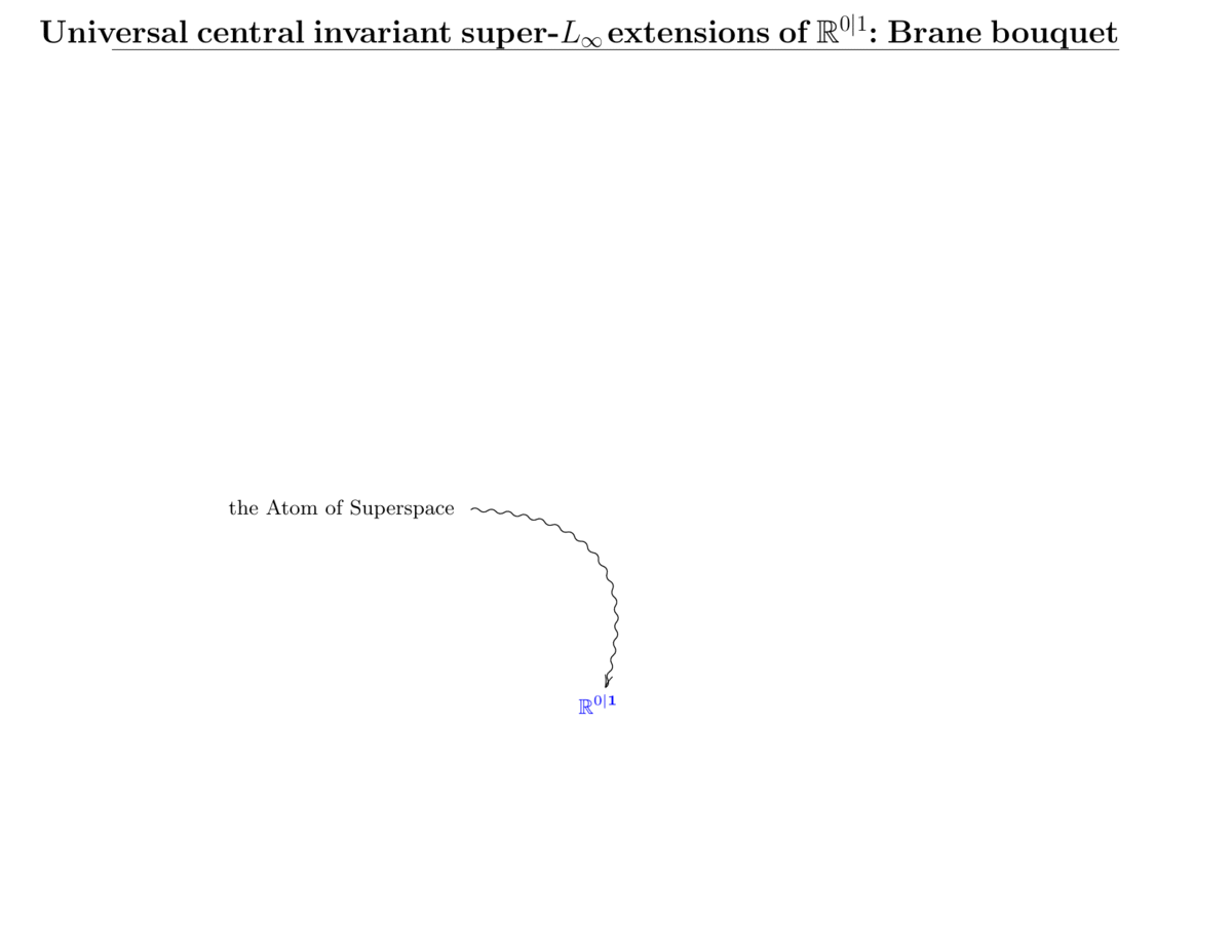
Super-branes emerge. When seen in the higher super-cohesive topos, these super-spacetimes sprout a whole bouquet of further invariant higher extensions [14] which may be understood [3] as (higher super-spacetimes extended by charges of) brane species: The brane bouquet [11][36, p. 14] shown in Figure 2. Notably, 11D super-space carries an invariant 4-cocycle which is the WZW term of the M2-brane sigma model, whence the higher central extension it classifies is known as $\mathfrak{m}2\mathfrak{brane}$ ([35, §3.1.3][11, Def. 4.2][36, p. 13] to be read as: “11D super-space extended by M2-brane charges”):

This, in turn, carries yet one more invariant 7-cocycle, being the WZW term of the M5-brane sigma model:

Figure 2 – The Brane Bouquet. In cohesive homotopy theory there emerges, from the super-point, a bouquet of (invariant central) higher extensions which first [37] grows the super-spacetimes in the critical dimensions of string theory, then [11] sprouts the corresponding super-brane species, and eventually blossoms into the M-brane species on 11D super-space classified in rational 4-Cohomotopy [12][13] (animated exposition in [86], more background in [14, Fig. 1][36, Fig. 3]). This is a “structural” or “synthetic” emergence of spacetime, which is possible in topos/type theory, quite distinct in nature from attempts to see spacetime emerge via point-set or graph models.

The C-field emerges. Finally, the abelian M2- and M5-brane cocycles unify [12, §3][14, (57)] into a single non-abelian cocycle in 4-Cohomotopy [13, Cor. 2.3], via homotopy pullback (cf. [19, Ex. 1.12]) along the Hopf fibration (5):

               

But this 4-Cohomotopy cocycle in 11D — which thus emerges from the super-point — is the avatar (in a precise sense, [24, Thm. 3.1]) of the C-field that we started the discussion with!, above in (3).

This may be seen to close a grand circle, where (super-)gravitational spacetime emerges from homotopical logic (§3), as such holographically exhibits topological qbits (§1), which in turn are naturally described in homotopy-typed language (§2).