Hair cells in the cochlea must tune resonant modes to the edge of instability without destabilizing collective modes

Asheesh S. Momi Department of Physics, Yale University, New Haven, CT 06520 Quantitative Biology Institute, Yale University, New Haven, CT 06520    Michael C. Abbott Department of Physics, Yale University, New Haven, CT 06520 Quantitative Biology Institute, Yale University, New Haven, CT 06520    Julian Rubinfien Department of Physics, Yale University, New Haven, CT 06520 Quantitative Biology Institute, Yale University, New Haven, CT 06520    Benjamin B. Machta benjamin.machta@yale.edu Department of Physics, Yale University, New Haven, CT 06520 Quantitative Biology Institute, Yale University, New Haven, CT 06520    Isabella R. Graf isabella.graf@embl.de Department of Physics, Yale University, New Haven, CT 06520 Quantitative Biology Institute, Yale University, New Haven, CT 06520 Developmental Biology Unit, European Molecular Biology Laboratory, 69117 Heidelberg, Germany
(19 July 2024. v2: 18 December 2024)
Abstract

Sound produces surface waves along the cochlea’s basilar membrane. To achieve the ear’s astonishing frequency resolution and sensitivity to faint sounds, dissipation in the cochlea must be canceled via active processes in hair cells, effectively bringing the cochlea to the edge of instability. But how can the cochlea be globally tuned to the edge of instability with only local feedback? To address this question, we use a discretized version of a standard model of basilar membrane dynamics, but with an explicit contribution from active processes in hair cells. Surprisingly, we find the basilar membrane supports two qualitatively distinct sets of modes: a continuum of localized modes and a small number of collective extended modes. Localized modes sharply peak at their resonant position and are largely uncoupled. As a result, they can be amplified almost independently from each other by local hair cells via feedback reminiscent of self-organized criticality. However, this amplification can destabilize the collective extended modes; avoiding such instabilities places limits on possible molecular mechanisms for active feedback in hair cells. Our work illuminates how and under what conditions individual hair cells can collectively create a critical cochlea.

Introduction

The human cochlea is a spiral-shaped organ in the inner ear, where sound is converted into electrical signals. The cochlea can detect sounds with frequencies across three orders of magnitude (20–20 000Hz) and more than a trillion-fold range in power (0–130dB), down to air vibrations on the order of an angstrom. After entering the cochlea, sound waves become surface waves along the basilar membrane (BM), depositing most incident energy in a frequency-specific location reichenbach2014physics .
To appear in PRX Life, accepted 5 December 2024.

Dissipation in the cochlea, through friction and viscous loss, limits frequency resolution and sensitivity. To counter dissipation, the cochlea contains active force-generating mechanisms kemp1979evidence ; dallos1992active ; martin1999active ; ren2011measurement . Active processes are performed by hair cells, small sensory structures that line the BM. For overly strong hair cell activity, the BM becomes unstable to spontaneous oscillations. When activity almost cancels friction, the cochlea is highly sensitive to weak amplitude signals, and frequency selectivity is high. This barely-stable regime is thus ideal for sound processing, but appears to require fine-tuning. Here we ask how hair cells can find this operating regime.

Past models have provided insight into possible mechanisms for tuning individual hair cells nadrowski2004active ; roongthumskul2011multiple ; camalet2000auditory . In particular, these papers studied how single hair cells can find a Hopf bifurcation, a transition between a stable and an unstable oscillatory regime. The discussion often focuses on bullfrog hearing where there is no cochlea, and hair cells act as relatively independent mechanical oscillators eatock1987adaptation . Conversely, models of the mammalian cochlea typically ignore tuning and operate under the assumption that active processes have globally reduced friction to near zero Julicher2003 .

In this work, we argue that assuming that hair cells cancel friction for all frequencies and positions is neither necessary nor feasible, and we instead seek to understand how they can find an operating region with the desired properties of the dissipation-free state. Friction only dominates the dynamics of the cochlea precisely at resonance because passive mechanics are underdamped lighthill1981energy . Furthermore, individual hair cells are small mechanical perturbations to the overall dynamics and their contribution to the non-dissipative mechanics is likely inconsequential. We thus focus on the role of hair cell activity in reducing friction in a manner which is local in both space and frequency. We show that, with some interesting caveats, this is sufficient to bring the cochlea to a line of Hopf bifurcations where every frequency is nearly critical at a specific location talmadge1993new ; eguiluz2000essential .

Towards this end we expand on an established model for the dynamics of the cochlea reichenbach2014physics ; Julicher2003 ; talmadge1998modeling , by explicitly adding mechanical contributions from active processes in hair cells. We assume that hair cells detect the displacement of the BM and respond by exerting forces via a fast linear response kernel. Each hair cell can also slowly adjust the strength of its active processes to find the global operating regime.

Perhaps surprisingly, this model of the cochlea contains two distinct types of modes. The first type, which we term localized modes, strongly peak at particular resonant positions. The second type instead have energy throughout the cochlea, reminiscent of standing waves, and we term them extended modes. Both types of modes are present in the passive system, and tuning activity is generally able to bring the localized modes to the edge of instability. By contrast, the extended modes become unstable for many plausible forms of active processes. For suitable forms of active processes, we further propose a mechanism reminiscent of self-organized criticality sornette_critical_1992 ; sornette_mapping_1995 , which tunes the local activity strength to the edge of instability.

Refer to caption
Figure 1: Schematic of the model. Above, we unroll the spiral-shaped cochlea into a model of two fluid-filled chambers partitioned by the basilar membrane (BM). Pressure waves in the fluid are accompanied by BM displacement h(x,t)𝑥𝑡h(x,t)italic_h ( italic_x , italic_t ), which we model as a set of N𝑁Nitalic_N damped harmonic oscillators, each with active driving from a hair cell. Sound input from the middle ear is via the displacement dow(t)subscript𝑑ow𝑡d_{\mathrm{ow}}(t)italic_d start_POSTSUBSCRIPT roman_ow end_POSTSUBSCRIPT ( italic_t ) of the oval window (OW) and a corresponding flux at the cochlea’s base, which due to fluid incompressibility causes an equal and opposite flux at the round window (RW). The pressure difference at the helicotrema at x=L𝑥𝐿x=Litalic_x = italic_L is set to zero.

Results

The passive part of our model of the cochlea has three components: the fluid which moves along the cochlea, the oval window by which the middle ear pushes this fluid, and the elastic basilar membrane which separates the cochlea into two compartments. We introduce each of these in turn and examine the resulting mode structure, before focusing on the active component, hair cells. Our mode computation uses a discretization of the BM into N𝑁Nitalic_N components, as shown in Fig. 1, but to describe the fluid it is clearer to start with a continuous position x𝑥xitalic_x along the BM.

Wave equation for the cochlea

The passive model we use is based primarily on the model from Ref. talmadge1998modeling , but also shares similarities with the models from Refs. reichenbach2014physics ; Julicher2003 . In line with these previous models, we approximate the cochlea as two fluid-filled compartments, the scala tympani and the scala vestibuli, which are separated by the BM (Fig. 1). Sound creates a fluid flux, coupled to a change in pressure described by force balance:

ρtj(x,t)=Acsxp(x,t).𝜌subscript𝑡𝑗𝑥𝑡subscript𝐴cssubscript𝑥𝑝𝑥𝑡\rho\partial_{t}j(x,t)=-A_{\text{cs}}\partial_{x}p(x,t).italic_ρ ∂ start_POSTSUBSCRIPT italic_t end_POSTSUBSCRIPT italic_j ( italic_x , italic_t ) = - italic_A start_POSTSUBSCRIPT cs end_POSTSUBSCRIPT ∂ start_POSTSUBSCRIPT italic_x end_POSTSUBSCRIPT italic_p ( italic_x , italic_t ) . (1)

Here, j(x,t)𝑗𝑥𝑡j(x,t)italic_j ( italic_x , italic_t ) is the difference in volume current between the lower and upper compartment, p(x,t)𝑝𝑥𝑡p(x,t)italic_p ( italic_x , italic_t ) is the pressure difference, Acssubscript𝐴csA_{\text{cs}}italic_A start_POSTSUBSCRIPT cs end_POSTSUBSCRIPT is the average cross-sectional area of a cochlear compartment, and ρ𝜌\rhoitalic_ρ is the density of water. The fluid flux propagates down the cochlea, creating a displacement of the BM, h(x,t)𝑥𝑡h(x,t)italic_h ( italic_x , italic_t ), which we call its height. The fluid flux obeys a continuity equation,

2Wbmth(x,t)+xj(x,t)=0,2subscript𝑊bmsubscript𝑡𝑥𝑡subscript𝑥𝑗𝑥𝑡02W_{\text{bm}}\partial_{t}h(x,t)+\partial_{x}j(x,t)=0,2 italic_W start_POSTSUBSCRIPT bm end_POSTSUBSCRIPT ∂ start_POSTSUBSCRIPT italic_t end_POSTSUBSCRIPT italic_h ( italic_x , italic_t ) + ∂ start_POSTSUBSCRIPT italic_x end_POSTSUBSCRIPT italic_j ( italic_x , italic_t ) = 0 , (2)

where Wbmsubscript𝑊bmW_{\text{bm}}italic_W start_POSTSUBSCRIPT bm end_POSTSUBSCRIPT is the width of the BM. We can eliminate j(x,t)𝑗𝑥𝑡j(x,t)italic_j ( italic_x , italic_t ) from Eq. 1 and 2 to arrive at a modified wave equation relating height and pressure Julicher2003 ; talmadge1998modeling ; reichenbach2014physics ,

2ρWbmAcst2h(x,t)=x2p(x,t).2𝜌subscript𝑊bmsubscript𝐴cssuperscriptsubscript𝑡2𝑥𝑡superscriptsubscript𝑥2𝑝𝑥𝑡\frac{2\rho W_{\text{bm}}}{A_{\text{cs}}}\partial_{t}^{2}h(x,t)=\partial_{x}^{% 2}p(x,t).divide start_ARG 2 italic_ρ italic_W start_POSTSUBSCRIPT bm end_POSTSUBSCRIPT end_ARG start_ARG italic_A start_POSTSUBSCRIPT cs end_POSTSUBSCRIPT end_ARG ∂ start_POSTSUBSCRIPT italic_t end_POSTSUBSCRIPT start_POSTSUPERSCRIPT 2 end_POSTSUPERSCRIPT italic_h ( italic_x , italic_t ) = ∂ start_POSTSUBSCRIPT italic_x end_POSTSUBSCRIPT start_POSTSUPERSCRIPT 2 end_POSTSUPERSCRIPT italic_p ( italic_x , italic_t ) . (3)

Sound enters the cochlea through the oval window, which connects to the middle ear and, in turn, the ear canal. We follow Ref. talmadge1998modeling for the boundary conditions at the base of the cochlea (x=0𝑥0x=0italic_x = 0), where the lateral displacement of the oval window dow(t)subscript𝑑ow𝑡d_{\mathrm{ow}}(t)italic_d start_POSTSUBSCRIPT roman_ow end_POSTSUBSCRIPT ( italic_t ) creates a flux of fluid, and eventually an equal and opposite flux in the scala tympani’s round window. Via Eq. 1, this leads to a pressure gradient:

t2dow(t)=12Aowtj(0,t)=Acs2ρAowxp(0,t).superscriptsubscript𝑡2subscript𝑑ow𝑡12subscript𝐴owsubscript𝑡𝑗0𝑡subscript𝐴cs2𝜌subscript𝐴owsubscript𝑥𝑝0𝑡\partial_{t}^{2}{d}_{\text{ow}}(t)=-\frac{1}{2A_{\text{ow}}}\partial_{t}j(0,t)% =\frac{A_{\text{cs}}}{2\rho A_{\text{ow}}}\partial_{x}p(0,t).∂ start_POSTSUBSCRIPT italic_t end_POSTSUBSCRIPT start_POSTSUPERSCRIPT 2 end_POSTSUPERSCRIPT italic_d start_POSTSUBSCRIPT ow end_POSTSUBSCRIPT ( italic_t ) = - divide start_ARG 1 end_ARG start_ARG 2 italic_A start_POSTSUBSCRIPT ow end_POSTSUBSCRIPT end_ARG ∂ start_POSTSUBSCRIPT italic_t end_POSTSUBSCRIPT italic_j ( 0 , italic_t ) = divide start_ARG italic_A start_POSTSUBSCRIPT cs end_POSTSUBSCRIPT end_ARG start_ARG 2 italic_ρ italic_A start_POSTSUBSCRIPT ow end_POSTSUBSCRIPT end_ARG ∂ start_POSTSUBSCRIPT italic_x end_POSTSUBSCRIPT italic_p ( 0 , italic_t ) . (4)

Here Aowsubscript𝐴owA_{\mathrm{ow}}italic_A start_POSTSUBSCRIPT roman_ow end_POSTSUBSCRIPT is the area of the oval window. The oval window itself acts as a damped harmonic oscillator:

t2dow(t)+ξowtdow(t)+ωow2dow(t)=p(0,t)+GmePec(t)σow,superscriptsubscript𝑡2subscript𝑑ow𝑡subscript𝜉owsubscript𝑡subscript𝑑ow𝑡superscriptsubscript𝜔ow2subscript𝑑ow𝑡𝑝0𝑡subscript𝐺mesubscript𝑃ec𝑡subscript𝜎ow\partial_{t}^{2}{d}_{\mathrm{ow}}(t)+\xi_{\mathrm{ow}}\partial_{t}{d}_{\mathrm% {ow}}(t)+\omega_{\mathrm{ow}}^{2}d_{\mathrm{ow}}(t)=\frac{p(0,t)+G_{\mathrm{me% }}P_{\mathrm{ec}}(t)}{\sigma_{\mathrm{ow}}},∂ start_POSTSUBSCRIPT italic_t end_POSTSUBSCRIPT start_POSTSUPERSCRIPT 2 end_POSTSUPERSCRIPT italic_d start_POSTSUBSCRIPT roman_ow end_POSTSUBSCRIPT ( italic_t ) + italic_ξ start_POSTSUBSCRIPT roman_ow end_POSTSUBSCRIPT ∂ start_POSTSUBSCRIPT italic_t end_POSTSUBSCRIPT italic_d start_POSTSUBSCRIPT roman_ow end_POSTSUBSCRIPT ( italic_t ) + italic_ω start_POSTSUBSCRIPT roman_ow end_POSTSUBSCRIPT start_POSTSUPERSCRIPT 2 end_POSTSUPERSCRIPT italic_d start_POSTSUBSCRIPT roman_ow end_POSTSUBSCRIPT ( italic_t ) = divide start_ARG italic_p ( 0 , italic_t ) + italic_G start_POSTSUBSCRIPT roman_me end_POSTSUBSCRIPT italic_P start_POSTSUBSCRIPT roman_ec end_POSTSUBSCRIPT ( italic_t ) end_ARG start_ARG italic_σ start_POSTSUBSCRIPT roman_ow end_POSTSUBSCRIPT end_ARG , (5)

where ξowsubscript𝜉ow\xi_{\text{ow}}italic_ξ start_POSTSUBSCRIPT ow end_POSTSUBSCRIPT is its dampening constant, ωowsubscript𝜔ow\omega_{\text{ow}}italic_ω start_POSTSUBSCRIPT ow end_POSTSUBSCRIPT the middle ear resonance, Pec(t)subscript𝑃ec𝑡P_{\text{ec}}(t)italic_P start_POSTSUBSCRIPT ec end_POSTSUBSCRIPT ( italic_t ) the pressure in the ear canal, Gmesubscript𝐺meG_{\text{me}}italic_G start_POSTSUBSCRIPT me end_POSTSUBSCRIPT the gain of the middle ear, and σowsubscript𝜎ow\sigma_{\text{ow}}italic_σ start_POSTSUBSCRIPT ow end_POSTSUBSCRIPT the mass per area of the oval window. At the cochlea’s apex (x=L𝑥𝐿x=Litalic_x = italic_L), a gap in the basilar membrane (the helicotrema) suggests zero pressure difference talmadge1998modeling :

p(L,t)=0.𝑝𝐿𝑡0p(L,t)=0.italic_p ( italic_L , italic_t ) = 0 . (6)

Resonance from passive impedance

To relate the height and pressure in Eq. 3, we need a mechanical model of the basilar membrane and its surrounding fluid. As is commonly assumed, we take the relationship to be local in space, where it can be written in the frequency domain via the acoustic impedance talmadge1993new :

p~(x,ω)=Z(x,ω)h~(x,ω)σbm,~𝑝𝑥𝜔𝑍𝑥𝜔~𝑥𝜔subscript𝜎bm\tilde{p}(x,\omega)=Z(x,\omega)\tilde{h}(x,\omega)\sigma_{\text{bm}},over~ start_ARG italic_p end_ARG ( italic_x , italic_ω ) = italic_Z ( italic_x , italic_ω ) over~ start_ARG italic_h end_ARG ( italic_x , italic_ω ) italic_σ start_POSTSUBSCRIPT bm end_POSTSUBSCRIPT , (7)

where σbmsubscript𝜎bm\sigma_{\mathrm{bm}}italic_σ start_POSTSUBSCRIPT roman_bm end_POSTSUBSCRIPT is the mass per area of the BM. Here, we separate the impedance Z(x,ω)=Zhc(x,ω)+Zpas(x,ω)𝑍𝑥𝜔subscript𝑍hc𝑥𝜔subscript𝑍pas𝑥𝜔Z(x,\omega)=Z_{\mathrm{hc}}(x,\omega)+Z_{\mathrm{pas}}(x,\omega)italic_Z ( italic_x , italic_ω ) = italic_Z start_POSTSUBSCRIPT roman_hc end_POSTSUBSCRIPT ( italic_x , italic_ω ) + italic_Z start_POSTSUBSCRIPT roman_pas end_POSTSUBSCRIPT ( italic_x , italic_ω ) into an active component due to hair cells, and the commonly used passive components due to stiffness, inertia, and friction:

Zpas(x,ω)=ω02e2kxω2+iξω.subscript𝑍pas𝑥𝜔superscriptsubscript𝜔02superscript𝑒2𝑘𝑥superscript𝜔2𝑖𝜉𝜔Z_{\mathrm{pas}}(x,\omega)=\omega_{0}^{2}e^{-2kx}-\omega^{2}+i\xi\omega.italic_Z start_POSTSUBSCRIPT roman_pas end_POSTSUBSCRIPT ( italic_x , italic_ω ) = italic_ω start_POSTSUBSCRIPT 0 end_POSTSUBSCRIPT start_POSTSUPERSCRIPT 2 end_POSTSUPERSCRIPT italic_e start_POSTSUPERSCRIPT - 2 italic_k italic_x end_POSTSUPERSCRIPT - italic_ω start_POSTSUPERSCRIPT 2 end_POSTSUPERSCRIPT + italic_i italic_ξ italic_ω . (8)

The stiffness decays exponentially in space emadi2004stiffness ; greenwood1990cochlear , with ω0subscript𝜔0\omega_{0}italic_ω start_POSTSUBSCRIPT 0 end_POSTSUBSCRIPT denoting the resonant frequency at the base of the cochlea. We deviate from the model of Ref. talmadge1998modeling by treating ξ𝜉\xiitalic_ξ, the dampening per unit mass, as constant for simplicity. A tilde represents a temporal Fourier transform ϕ~(ω)=𝑑teiωtϕ(t)~italic-ϕ𝜔differential-d𝑡superscript𝑒𝑖𝜔𝑡italic-ϕ𝑡\tilde{\phi}(\omega)=\int dte^{-i\omega t}\phi(t)over~ start_ARG italic_ϕ end_ARG ( italic_ω ) = ∫ italic_d italic_t italic_e start_POSTSUPERSCRIPT - italic_i italic_ω italic_t end_POSTSUPERSCRIPT italic_ϕ ( italic_t ). Table 1 lists all the constants in this model.

The passive components of BM impedance lead to the most important feature of cochlear mechanics: spatial frequency discrimination. Resonances occur when the two real contributions to Zpassubscript𝑍pasZ_{\mathrm{pas}}italic_Z start_POSTSUBSCRIPT roman_pas end_POSTSUBSCRIPT cancel, which happens at a position-dependent resonant frequency

ωrespas(x)=ω0ekx.superscriptsubscript𝜔respas𝑥subscript𝜔0superscript𝑒𝑘𝑥\omega_{\mathrm{res}}^{\mathrm{pas}}(x)=\omega_{0}e^{-kx}.italic_ω start_POSTSUBSCRIPT roman_res end_POSTSUBSCRIPT start_POSTSUPERSCRIPT roman_pas end_POSTSUPERSCRIPT ( italic_x ) = italic_ω start_POSTSUBSCRIPT 0 end_POSTSUBSCRIPT italic_e start_POSTSUPERSCRIPT - italic_k italic_x end_POSTSUPERSCRIPT . (9)

There Zpassubscript𝑍pasZ_{\mathrm{pas}}italic_Z start_POSTSUBSCRIPT roman_pas end_POSTSUBSCRIPT is purely imaginary. If it were zero, a small change in pressure would result in an infinite change in height, and thus Z(x,ω)=0𝑍𝑥𝜔0Z(x,\omega)=0italic_Z ( italic_x , italic_ω ) = 0 is a critical point. However, in the real cochlea, a non-zero imaginary part due to friction limits the amplitude of near-resonant displacements. And while the imaginary part of the passive impedance is typically two orders of magnitude smaller than both contributions to the real part talmadge1998modeling , it does become significant near the resonant frequency martin2021mechanical ; iwasa1997force . Since no passive properties can cancel it, hair cells must exert active forces to oppose friction and achieve higher sensitivity.

Symbol Value Description
ρ𝜌\rhoitalic_ρ 103kg/m3superscript103kgsuperscriptm310^{3}~{}$\mathrm{k}\mathrm{g}\mathrm{/}\,\mathrm{m}^{3}$10 start_POSTSUPERSCRIPT 3 end_POSTSUPERSCRIPT roman_kg / roman_m start_POSTSUPERSCRIPT 3 end_POSTSUPERSCRIPT Density of water
Acssubscript𝐴csA_{\text{cs}}italic_A start_POSTSUBSCRIPT cs end_POSTSUBSCRIPT 1.1×10⁶m21.1superscript106superscriptm21.1\times 10^{-6}~{}$\mathrm{m}^{2}$1.1 × 10 start_POSTSUPERSCRIPT - 6 end_POSTSUPERSCRIPT roman_m start_POSTSUPERSCRIPT 2 end_POSTSUPERSCRIPT Average cross-sectional area of a cochlear partition
Aowsubscript𝐴owA_{\text{ow}}italic_A start_POSTSUBSCRIPT ow end_POSTSUBSCRIPT 3.2×10⁶m23.2superscript106superscriptm23.2\times 10^{-6}~{}$\mathrm{m}^{2}$3.2 × 10 start_POSTSUPERSCRIPT - 6 end_POSTSUPERSCRIPT roman_m start_POSTSUPERSCRIPT 2 end_POSTSUPERSCRIPT Area of oval window (OW)
Wbmsubscript𝑊bmW_{\text{bm}}italic_W start_POSTSUBSCRIPT bm end_POSTSUBSCRIPT 2.9×10⁴m2.9superscript104m2.9\times 10^{-4}~{}$\mathrm{m}$2.9 × 10 start_POSTSUPERSCRIPT - 4 end_POSTSUPERSCRIPT roman_m Average width of the BM
ξowsubscript𝜉ow\xi_{\text{ow}}italic_ξ start_POSTSUBSCRIPT ow end_POSTSUBSCRIPT 500s1500superscripts1500~{}$\mathrm{s}^{-1}$500 roman_s start_POSTSUPERSCRIPT - 1 end_POSTSUPERSCRIPT OW dampening constant
ξ𝜉\xiitalic_ξ 100s1100superscripts1100~{}$\mathrm{s}^{-1}$100 roman_s start_POSTSUPERSCRIPT - 1 end_POSTSUPERSCRIPT BM dampening constant
ωowsubscript𝜔ow\omega_{\text{ow}}italic_ω start_POSTSUBSCRIPT ow end_POSTSUBSCRIPT 2π×1500rad/s2𝜋1500rads2\pi\times 1500~{}$\mathrm{r}\mathrm{a}\mathrm{d}\mathrm{/}\mathrm{s}$2 italic_π × 1500 roman_rad / roman_s OW resonant frequency
ω0subscript𝜔0\omega_{0}italic_ω start_POSTSUBSCRIPT 0 end_POSTSUBSCRIPT 2π×20800rad/s2𝜋20800rads2\pi\times 20800~{}$\mathrm{r}\mathrm{a}\mathrm{d}\mathrm{/}\mathrm{s}$2 italic_π × 20800 roman_rad / roman_s Highest resonant frequency of the BM
k𝑘kitalic_k 1.38×10²m11.38superscript102superscriptm11.38\times 10^{2}~{}$\mathrm{m}^{-1}$1.38 × 10 start_POSTSUPERSCRIPT 2 end_POSTSUPERSCRIPT roman_m start_POSTSUPERSCRIPT - 1 end_POSTSUPERSCRIPT Stiffness decay coefficient
σowsubscript𝜎ow\sigma_{\text{ow}}italic_σ start_POSTSUBSCRIPT ow end_POSTSUBSCRIPT 18.5kg/m218.5kgsuperscriptm218.5~{}$\mathrm{k}\mathrm{g}\mathrm{/}\mathrm{m}^{2}$18.5 roman_kg / roman_m start_POSTSUPERSCRIPT 2 end_POSTSUPERSCRIPT Effective areal density of the OW
σbmsubscript𝜎bm\sigma_{\text{bm}}italic_σ start_POSTSUBSCRIPT bm end_POSTSUBSCRIPT 5.5×10²kg/m25.5superscript102kgsuperscriptm25.5\times 10^{-2}~{}$\mathrm{k}\mathrm{g}\mathrm{/}\mathrm{m}^{2}$5.5 × 10 start_POSTSUPERSCRIPT - 2 end_POSTSUPERSCRIPT roman_kg / roman_m start_POSTSUPERSCRIPT 2 end_POSTSUPERSCRIPT Areal density of the BM
Gmesubscript𝐺meG_{\text{me}}italic_G start_POSTSUBSCRIPT me end_POSTSUBSCRIPT 21.421.421.421.4 Gain of the middle ear
L𝐿Litalic_L 3.5×10²m3.5superscript102m3.5\times 10^{-2}~{}$\mathrm{m}$3.5 × 10 start_POSTSUPERSCRIPT - 2 end_POSTSUPERSCRIPT roman_m Length of the BM
Table 1: Numerical parameters of the human cochlea used in Eq. 1-8. All parameter values are taken from Talmadge et al., Ref. talmadge1998modeling . Variants of their model with additional parameters are discussed in Appendix C.
Refer to caption
Figure 2: The cochlea exhibits a near-continuum of localized modes plus a discrete set of extended low-frequency modes. (A) The eigenvalue structure of oscillating cochlear modes. An eigenvalue’s imaginary part determines the oscillation frequency, and the real part determines stability. We define the localized modes (red) as the ones which have a resonant position within the cochlea, i.e., those for which |Im(λj)|>ωres(L)subscript𝜆𝑗subscript𝜔res𝐿\lvert\imaginary(\lambda_{j})\rvert>\omega_{\text{res}}(L)| start_OPERATOR roman_Im end_OPERATOR ( italic_λ start_POSTSUBSCRIPT italic_j end_POSTSUBSCRIPT ) | > italic_ω start_POSTSUBSCRIPT res end_POSTSUBSCRIPT ( italic_L ). Extended modes (blue) are those with |Im(λj)|<ωres(L)subscript𝜆𝑗subscript𝜔res𝐿\lvert\imaginary(\lambda_{j})\rvert<\omega_{\text{res}}(L)| start_OPERATOR roman_Im end_OPERATOR ( italic_λ start_POSTSUBSCRIPT italic_j end_POSTSUBSCRIPT ) | < italic_ω start_POSTSUBSCRIPT res end_POSTSUBSCRIPT ( italic_L ), so their resonant position would be past the end of the cochlea; e.g., the 18181818 Hz mode would be resonant at a position of x=5.1𝑥5.1x=5.1italic_x = 5.1 cm. There are 12121212 extended modes, and N12𝑁12N-12italic_N - 12 localized modes, approaching a continuum of resonant frequencies at large N𝑁Nitalic_N. The uncoupled system (gray) displays the eigenvalues of N𝑁Nitalic_N independent harmonic oscillators with stiffness, mass, friction, and active force identical to each BM segment (i.e. the roots of Z(xn,iλ)=0𝑍subscript𝑥𝑛𝑖𝜆0Z(x_{n},i\lambda)=0italic_Z ( italic_x start_POSTSUBSCRIPT italic_n end_POSTSUBSCRIPT , italic_i italic_λ ) = 0). (B) Eigenvectors corresponding to the circled eigenvalues. We show the localized modes for 1111 kHz and 10101010 kHz and the two lowest-frequency extended modes. (C) Colour map of normalized Im[Z(x,ω)]𝑍𝑥𝜔\imaginary[Z(x,\omega)]start_OPERATOR roman_Im end_OPERATOR [ italic_Z ( italic_x , italic_ω ) ], the effective net friction, across frequencies and position. On the left of resonance (dashed black line), active processes add more energy than passive friction removes, leading to a negative effective friction (orange). All plots have an active hair cell response kernel gerΔtproportional-to𝑔superscript𝑒𝑟Δ𝑡g\propto e^{-r\Delta t}italic_g ∝ italic_e start_POSTSUPERSCRIPT - italic_r roman_Δ italic_t end_POSTSUPERSCRIPT from Eq. 15 with α=2𝛼2\alpha=2italic_α = 2, C99(x)subscript𝐶99𝑥C_{99}(x)italic_C start_POSTSUBSCRIPT 99 end_POSTSUBSCRIPT ( italic_x ) from Eq. 13, and N=1000𝑁1000N=1000italic_N = 1000. Fig. 3 repeats panels A and C for other choices of response kernel g𝑔gitalic_g defined in Eqs. 15, 16, and 18.

Active hair cell contributions

The passive part of the model we have described so far closely follows previous models of the cochlea talmadge1998modeling ; Julicher2003 ; reichenbach2014physics . To take into account active processes, a common approach is to assume that they cancel friction for all frequencies and positions, equivalent to setting ξ=0𝜉0\xi=0italic_ξ = 0 Julicher2003 ; talmadge1998modeling . Implementing this strict condition would, however, require an instantaneous derivative response, discussed below.

Here, we instead allow hair cells to respond over a finite time. We write the active contribution from hair cells to Eq. 7 in terms of a generic linear response kernel g𝑔gitalic_g and a dimensionless strength C𝐶Citalic_C:

Zhc(x,ω)=C(x)g~(x,ω).subscript𝑍hc𝑥𝜔𝐶𝑥~𝑔𝑥𝜔Z_{\mathrm{hc}}(x,\omega)=C(x)\,\tilde{g}(x,\omega).italic_Z start_POSTSUBSCRIPT roman_hc end_POSTSUBSCRIPT ( italic_x , italic_ω ) = italic_C ( italic_x ) over~ start_ARG italic_g end_ARG ( italic_x , italic_ω ) . (10)

This term contributes an active pressure phcsubscript𝑝hcp_{\mathrm{hc}}italic_p start_POSTSUBSCRIPT roman_hc end_POSTSUBSCRIPT best understood in the time domain:

phc(x,t)=σbmC(x)0𝑑Δtg(x,Δt)h(x,tΔt).subscript𝑝hc𝑥𝑡subscript𝜎bm𝐶𝑥superscriptsubscript0differential-dΔ𝑡𝑔𝑥Δ𝑡𝑥𝑡Δ𝑡p_{\mathrm{hc}}(x,t)=\sigma_{\mathrm{bm}}C(x)\int_{0}^{\infty}d\Delta t\>g(x,% \Delta t)\>h(x,t-\Delta t).italic_p start_POSTSUBSCRIPT roman_hc end_POSTSUBSCRIPT ( italic_x , italic_t ) = italic_σ start_POSTSUBSCRIPT roman_bm end_POSTSUBSCRIPT italic_C ( italic_x ) ∫ start_POSTSUBSCRIPT 0 end_POSTSUBSCRIPT start_POSTSUPERSCRIPT ∞ end_POSTSUPERSCRIPT italic_d roman_Δ italic_t italic_g ( italic_x , roman_Δ italic_t ) italic_h ( italic_x , italic_t - roman_Δ italic_t ) . (11)

The response kernel g(x,Δt)𝑔𝑥Δ𝑡g(x,\Delta t)italic_g ( italic_x , roman_Δ italic_t ) characterizes the active force’s dependence on past displacement, and C(x)𝐶𝑥C(x)italic_C ( italic_x ) controls the strength of the hair-cell force. We initially take g(x,Δt)er(x)Δtproportional-to𝑔𝑥Δ𝑡superscript𝑒𝑟𝑥Δ𝑡g(x,\Delta t)\propto e^{-r(x)\Delta t}italic_g ( italic_x , roman_Δ italic_t ) ∝ italic_e start_POSTSUPERSCRIPT - italic_r ( italic_x ) roman_Δ italic_t end_POSTSUPERSCRIPT, indicating that the hair cell integrates height for a time of order 1/r(x)1𝑟𝑥1/r(x)1 / italic_r ( italic_x ). This dependence could model, for instance, the concentration of calcium ions which enter when hair cells are displaced and are pumped out at rate r𝑟ritalic_r, with the accumulated concentration inside the cell controlling molecular motors camalet2000auditory . To function at both high and low frequencies, we might expect the timescale to vary like 1/ωrespas(x)1superscriptsubscript𝜔respas𝑥1/\omega_{\mathrm{res}}^{\mathrm{pas}}(x)1 / italic_ω start_POSTSUBSCRIPT roman_res end_POSTSUBSCRIPT start_POSTSUPERSCRIPT roman_pas end_POSTSUPERSCRIPT ( italic_x ) along the BM, and we should certainly expect that different molecular mechanisms will be employed to respond at 200Hz vs 20kHz. Hair cell activity can perturb the resonant frequency away from ωrespas(x)superscriptsubscript𝜔respas𝑥\omega_{\mathrm{res}}^{\mathrm{pas}}(x)italic_ω start_POSTSUBSCRIPT roman_res end_POSTSUBSCRIPT start_POSTSUPERSCRIPT roman_pas end_POSTSUPERSCRIPT ( italic_x ), and in general we define ωres(x)subscript𝜔res𝑥\omega_{\mathrm{res}}(x)italic_ω start_POSTSUBSCRIPT roman_res end_POSTSUBSCRIPT ( italic_x ) by

Re[Z(x,ωres(x))]=0.𝑍𝑥subscript𝜔res𝑥0\real[Z(x,\omega_{\mathrm{res}}(x))]=0.start_OPERATOR roman_Re end_OPERATOR [ italic_Z ( italic_x , italic_ω start_POSTSUBSCRIPT roman_res end_POSTSUBSCRIPT ( italic_x ) ) ] = 0 . (12)

Adjusting the strength of hair cell activity C(x)𝐶𝑥C(x)italic_C ( italic_x ) is not sufficient to cancel friction for all x𝑥xitalic_x and ω𝜔\omegaitalic_ω, as the frequency dependence of Zhc(x,ω)subscript𝑍hc𝑥𝜔Z_{\mathrm{hc}}(x,\omega)italic_Z start_POSTSUBSCRIPT roman_hc end_POSTSUBSCRIPT ( italic_x , italic_ω ) comes from g~(x,ω)~𝑔𝑥𝜔\tilde{g}(x,\omega)over~ start_ARG italic_g end_ARG ( italic_x , italic_ω ) which does not in general match the linear passive term, iξω𝑖𝜉𝜔i\xi\omegaitalic_i italic_ξ italic_ω. But adjusting C(x)𝐶𝑥C(x)italic_C ( italic_x ) does allow us to set Z(x,ωres(x))=0𝑍𝑥subscript𝜔res𝑥0Z(x,\omega_{\mathrm{res}}(x))=0italic_Z ( italic_x , italic_ω start_POSTSUBSCRIPT roman_res end_POSTSUBSCRIPT ( italic_x ) ) = 0, cancelling friction along a line in the position-frequency plane. With some important caveats discussed below, we will show that this is sufficient to make the cochlea highly sensitive. To investigate the resulting properties, we assume for now that a fixed fraction f𝑓fitalic_f (usually 99%) of the passive friction is cancelled at the resonant frequency:

C100f(x)=fξωres(x)Im[g~(x,ωres(x))].subscript𝐶100𝑓𝑥𝑓𝜉subscript𝜔res𝑥~𝑔𝑥subscript𝜔res𝑥C_{100f}(x)=f\,\frac{-\xi\omega_{\mathrm{res}}(x)}{\ \imaginary[\tilde{g}(x,% \omega_{\mathrm{res}}(x))]}.italic_C start_POSTSUBSCRIPT 100 italic_f end_POSTSUBSCRIPT ( italic_x ) = italic_f divide start_ARG - italic_ξ italic_ω start_POSTSUBSCRIPT roman_res end_POSTSUBSCRIPT ( italic_x ) end_ARG start_ARG start_OPERATOR roman_Im end_OPERATOR [ over~ start_ARG italic_g end_ARG ( italic_x , italic_ω start_POSTSUBSCRIPT roman_res end_POSTSUBSCRIPT ( italic_x ) ) ] end_ARG . (13)

However, cancellation of a large fraction like f=0.99𝑓0.99f=0.99italic_f = 0.99 requires extreme fine-tuning, as a 2% increase in f𝑓fitalic_f would make the system unstable everywhere. Instead of fine-tuning C(x)𝐶𝑥C(x)italic_C ( italic_x ) directly, we will later show how hair cells can use local information to robustly tune C(x)𝐶𝑥C(x)italic_C ( italic_x ) to bring the cochlea to the edge of instability without fine-tuning. But first, we will discuss the qualitative behaviour of the model at C99(x)subscript𝐶99𝑥C_{99}(x)italic_C start_POSTSUBSCRIPT 99 end_POSTSUBSCRIPT ( italic_x ).

Mode structure of the cochlea

We took a numerical approach to better understand the features of our model, discretizing the BM into N𝑁Nitalic_N units located at xn=Ln/Nsubscript𝑥𝑛𝐿𝑛𝑁x_{n}=Ln/Nitalic_x start_POSTSUBSCRIPT italic_n end_POSTSUBSCRIPT = italic_L italic_n / italic_N. Eqs. 3,5 can then be written as a set of coupled first-order differential equations. In matrix form, these become tX=J^Xsubscript𝑡𝑋^𝐽𝑋\partial_{t}{X}=\hat{J}X∂ start_POSTSUBSCRIPT italic_t end_POSTSUBSCRIPT italic_X = over^ start_ARG italic_J end_ARG italic_X, where the state vector X𝑋Xitalic_X concatenates dow(t)subscript𝑑ow𝑡d_{\mathrm{ow}}(t)italic_d start_POSTSUBSCRIPT roman_ow end_POSTSUBSCRIPT ( italic_t ), h(xn,t)subscript𝑥𝑛𝑡h(x_{n},t)italic_h ( italic_x start_POSTSUBSCRIPT italic_n end_POSTSUBSCRIPT , italic_t ) for all n𝑛nitalic_n, their time-derivatives, and any additional entries needed to describe active processes (such as phc(xn,t)subscript𝑝hcsubscript𝑥𝑛𝑡p_{\mathrm{hc}}(x_{n},t)italic_p start_POSTSUBSCRIPT roman_hc end_POSTSUBSCRIPT ( italic_x start_POSTSUBSCRIPT italic_n end_POSTSUBSCRIPT , italic_t ) for the one-exponential kernel). Eq. A24 in Appendix A is the final result. Diagonalizing the Jacobian J^^𝐽\hat{J}over^ start_ARG italic_J end_ARG elliott2007state yields modes as eigenvectors with corresponding eigenvalues λjsubscript𝜆𝑗\lambda_{j}italic_λ start_POSTSUBSCRIPT italic_j end_POSTSUBSCRIPT.

Refer to caption
Figure 3: Extended mode stability constrains hair cell response kernels. We consider 3 families of response kernels g(x,Δt)𝑔𝑥Δ𝑡g(x,\Delta t)italic_g ( italic_x , roman_Δ italic_t ), with the left column showing one exponential with a decay rate r(x)𝑟𝑥r(x)italic_r ( italic_x ) adjusted by α𝛼\alphaitalic_α, Eq 15. The middle and right columns have sums of two exponentials whose rates are controlled by α1,α2subscript𝛼1subscript𝛼2\alpha_{1},\alpha_{2}italic_α start_POSTSUBSCRIPT 1 end_POSTSUBSCRIPT , italic_α start_POSTSUBSCRIPT 2 end_POSTSUBSCRIPT, with two different choices of additive constant, Eqs 16 and 18. (B) Stability phase diagrams, on which green and yellow points indicate parameters α1,α2subscript𝛼1subscript𝛼2\alpha_{1},\alpha_{2}italic_α start_POSTSUBSCRIPT 1 end_POSTSUBSCRIPT , italic_α start_POSTSUBSCRIPT 2 end_POSTSUBSCRIPT at which there are no eigenvalues with positive real part when hair cells are tuned to cancel 99% of passive friction on resonance, C(x)=C99(x)𝐶𝑥subscript𝐶99𝑥C(x)=C_{99}(x)italic_C ( italic_x ) = italic_C start_POSTSUBSCRIPT 99 end_POSTSUBSCRIPT ( italic_x ) from Eq. 13. If the hair cells are instead tuned to cancel 90% of passive friction (C90subscript𝐶90C_{90}italic_C start_POSTSUBSCRIPT 90 end_POSTSUBSCRIPT), then more cases become stable, indicated by orange points. If they cancel 100% of passive friction (C100subscript𝐶100C_{100}italic_C start_POSTSUBSCRIPT 100 end_POSTSUBSCRIPT), then only the green points are stable. Background colour indicates stability according to the criterion of having ImZ(x,ω)>0𝑍𝑥𝜔0\imaginary Z(x,\omega)>0start_OPERATOR roman_Im end_OPERATOR italic_Z ( italic_x , italic_ω ) > 0 for all ω<ωres(x)𝜔subscript𝜔res𝑥\omega<\omega_{\mathrm{res}}(x)italic_ω < italic_ω start_POSTSUBSCRIPT roman_res end_POSTSUBSCRIPT ( italic_x ). Points marked by large symbols are plotted in lower panels, always with C99(x)subscript𝐶99𝑥C_{99}(x)italic_C start_POSTSUBSCRIPT 99 end_POSTSUBSCRIPT ( italic_x ). (C) At a particular position x0=2.5cmsubscript𝑥02.5cmx_{0}=2.5\mathrm{cm}italic_x start_POSTSUBSCRIPT 0 end_POSTSUBSCRIPT = 2.5 roman_cm, we plot the relative net friction Ξnet(x,ω)subscriptΞnet𝑥𝜔\Xi_{\mathrm{net}}(x,\omega)roman_Ξ start_POSTSUBSCRIPT roman_net end_POSTSUBSCRIPT ( italic_x , italic_ω ), for frequencies ω𝜔\omegaitalic_ω above and below the resonance frequency ωres(x0)subscript𝜔ressubscript𝑥0\omega_{\mathrm{res}}(x_{0})italic_ω start_POSTSUBSCRIPT roman_res end_POSTSUBSCRIPT ( italic_x start_POSTSUBSCRIPT 0 end_POSTSUBSCRIPT ). By definition of C99subscript𝐶99C_{99}italic_C start_POSTSUBSCRIPT 99 end_POSTSUBSCRIPT, this is equal to 10.9910.991-0.991 - 0.99 at ω=ωres(x0)𝜔subscript𝜔ressubscript𝑥0\omega=\omega_{\mathrm{res}}(x_{0})italic_ω = italic_ω start_POSTSUBSCRIPT roman_res end_POSTSUBSCRIPT ( italic_x start_POSTSUBSCRIPT 0 end_POSTSUBSCRIPT ). The friction criterion states that any negative values at ω<ωres(x0)𝜔subscript𝜔ressubscript𝑥0\omega<\omega_{\mathrm{res}}(x_{0})italic_ω < italic_ω start_POSTSUBSCRIPT roman_res end_POSTSUBSCRIPT ( italic_x start_POSTSUBSCRIPT 0 end_POSTSUBSCRIPT ) will produce instability (red background). (D) Relative net friction for all x𝑥xitalic_x and ω𝜔\omegaitalic_ω. By definition of C99subscript𝐶99C_{99}italic_C start_POSTSUBSCRIPT 99 end_POSTSUBSCRIPT, this is 0.01 along the resonance line ω=ωres(x)𝜔subscript𝜔res𝑥\omega=\omega_{\mathrm{res}}(x)italic_ω = italic_ω start_POSTSUBSCRIPT roman_res end_POSTSUBSCRIPT ( italic_x ). Positive values (purple) indicate energy loss, while negative values (orange) indicate energy gain, potentially leading to instability. (E) Mode eigenvalues, for the same selected parameters α1,α2subscript𝛼1subscript𝛼2\alpha_{1},\alpha_{2}italic_α start_POSTSUBSCRIPT 1 end_POSTSUBSCRIPT , italic_α start_POSTSUBSCRIPT 2 end_POSTSUBSCRIPT indicated by large symbols on the phase diagrams. Any eigenvalue with Re(λj)>0subscript𝜆𝑗0\real(\lambda_{j})>0start_OPERATOR roman_Re end_OPERATOR ( italic_λ start_POSTSUBSCRIPT italic_j end_POSTSUBSCRIPT ) > 0 is an unstable mode (red background). Eigenvalues in panels B, E were calculated at N=1000𝑁1000N=1000italic_N = 1000.

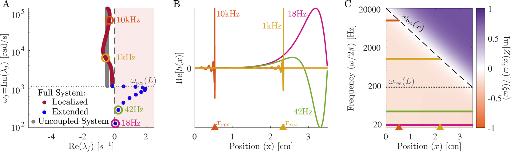
We find, perhaps surprisingly, that the eigenmodes fall into two qualitatively distinct classes, which we term localized and extended modes, whose eigenvalues and eigenvectors are plotted in Fig. 2. Each localized mode is strongly peaked at a specific location within the cochlea (orange and yellow in Fig. 2B), and the location xres<Lsubscript𝑥res𝐿x_{\mathrm{res}}<Litalic_x start_POSTSUBSCRIPT roman_res end_POSTSUBSCRIPT < italic_L of this peak is determined by its frequency ωj=Im[λj]subscript𝜔𝑗subscript𝜆𝑗\omega_{j}=\imaginary[\lambda_{j}]italic_ω start_POSTSUBSCRIPT italic_j end_POSTSUBSCRIPT = start_OPERATOR roman_Im end_OPERATOR [ italic_λ start_POSTSUBSCRIPT italic_j end_POSTSUBSCRIPT ]. But there are a few additional eigenvalues with ωj<ωres(L)subscript𝜔𝑗subscript𝜔res𝐿\omega_{j}<\omega_{\mathrm{res}}(L)italic_ω start_POSTSUBSCRIPT italic_j end_POSTSUBSCRIPT < italic_ω start_POSTSUBSCRIPT roman_res end_POSTSUBSCRIPT ( italic_L ) (blue points in Fig. 2A), which correspond to spatially extended eigenmodes (pink and green in Fig. 2B). Increasing the discretization scale N𝑁Nitalic_N increases the number of localized modes, without much effect on either the number of extended modes present (12 in the figure), or their frequencies.

The localized modes have been studied in detail reichenbach2014physics ; hudspeth2010critique ; talmadge1998modeling , and their sharpness in frequency and space is responsible for the remarkable precision with which we can sense pitch. Numerically, we find that the jthsuperscript𝑗𝑡j^{th}italic_j start_POSTSUPERSCRIPT italic_t italic_h end_POSTSUPERSCRIPT mode is peaked near the resonant position of its eigenvalue, xreslog(ω0/ωj)/ksubscript𝑥ressubscript𝜔0subscript𝜔𝑗𝑘x_{\mathrm{res}}\approx\log(\omega_{0}/\omega_{j})/kitalic_x start_POSTSUBSCRIPT roman_res end_POSTSUBSCRIPT ≈ roman_log ( start_ARG italic_ω start_POSTSUBSCRIPT 0 end_POSTSUBSCRIPT / italic_ω start_POSTSUBSCRIPT italic_j end_POSTSUBSCRIPT end_ARG ) / italic_k where ωj=|Imλj|subscript𝜔𝑗subscript𝜆𝑗\omega_{j}=\lvert\imaginary\lambda_{j}\rvertitalic_ω start_POSTSUBSCRIPT italic_j end_POSTSUBSCRIPT = | start_OPERATOR roman_Im end_OPERATOR italic_λ start_POSTSUBSCRIPT italic_j end_POSTSUBSCRIPT |. In the widely used and qualitatively accurate WKB approximation, the sharp peak at a given frequency is h(x,t)|Z(x,ωj)|3/4similar-to𝑥𝑡superscript𝑍𝑥subscript𝜔𝑗34h(x,t)\sim\lvert Z(x,\omega_{j})\rvert^{-3/4}italic_h ( italic_x , italic_t ) ∼ | italic_Z ( italic_x , italic_ω start_POSTSUBSCRIPT italic_j end_POSTSUBSCRIPT ) | start_POSTSUPERSCRIPT - 3 / 4 end_POSTSUPERSCRIPT. Waves approaching from the oval window (x=0𝑥0x=0italic_x = 0) have a decreasing wave speed as they travel right. They slow to zero at xressubscript𝑥resx_{\mathrm{res}}italic_x start_POSTSUBSCRIPT roman_res end_POSTSUBSCRIPT, and deposit most of their energy in a so-called critical layer, leaving only an evanescent wave to the right of resonance lighthill1981energy . Therefore, the stability of these modes is essentially determined by the stability of the local oscillator at resonance. So long as Im[Z(xres,ωj])]>0\imaginary[Z(x_{\mathrm{res}},\omega_{j}])]>0start_OPERATOR roman_Im end_OPERATOR [ italic_Z ( italic_x start_POSTSUBSCRIPT roman_res end_POSTSUBSCRIPT , italic_ω start_POSTSUBSCRIPT italic_j end_POSTSUBSCRIPT ] ) ] > 0, active processes are adding in less energy than friction is removing, and these modes are stable, Re(λj)<0subscript𝜆𝑗0\real(\lambda_{j})<0start_OPERATOR roman_Re end_OPERATOR ( italic_λ start_POSTSUBSCRIPT italic_j end_POSTSUBSCRIPT ) < 0. In the limit of Im[Z(xres,ωj)]0𝑍subscript𝑥ressubscript𝜔𝑗0\imaginary[Z(x_{\mathrm{res}},\omega_{j})]\rightarrow 0start_OPERATOR roman_Im end_OPERATOR [ italic_Z ( italic_x start_POSTSUBSCRIPT roman_res end_POSTSUBSCRIPT , italic_ω start_POSTSUBSCRIPT italic_j end_POSTSUBSCRIPT ) ] → 0, these modes become infinitely peaked, and they can be thought of as essentially uncoupled oscillators acting independently, whose eigenvalues are the roots of Z(xn,iλ)=0𝑍subscript𝑥𝑛𝑖𝜆0Z(x_{n},i\lambda)=0italic_Z ( italic_x start_POSTSUBSCRIPT italic_n end_POSTSUBSCRIPT , italic_i italic_λ ) = 0 (grey points in Fig. 2A). We anticipate that these modes can thus be tuned independently and brought to the edge of instability by choosing C(x)C100(x)𝐶𝑥subscript𝐶100𝑥C(x)\approx C_{100}(x)italic_C ( italic_x ) ≈ italic_C start_POSTSUBSCRIPT 100 end_POSTSUBSCRIPT ( italic_x ).

By contrast, the extended modes we find are inherently collective. They are defined by having frequencies below the lowest resonant frequency of the cochlea, |Im(λj)|<ωres(L)subscript𝜆𝑗subscript𝜔res𝐿\lvert\imaginary(\lambda_{j})\rvert<\omega_{\mathrm{res}}(L)| start_OPERATOR roman_Im end_OPERATOR ( italic_λ start_POSTSUBSCRIPT italic_j end_POSTSUBSCRIPT ) | < italic_ω start_POSTSUBSCRIPT roman_res end_POSTSUBSCRIPT ( italic_L ). These waves travel down the entire cochlea with no evanescent region and can be thought of as sums of right- and left-moving waves that reflect off of the boundary conditions at x=0,L𝑥0𝐿x=0,Litalic_x = 0 , italic_L. As with a more traditional wave equation, there is a single standing wave mode with no zero crossings (pink in Fig. 2B), one with a single zero crossing (green in Fig. 2B) and so on, with each successive mode having one more zero crossing and a higher characteristic frequency. However, this pattern is cut off at a small number of crossings, corresponding to the maximum frequency still below the resonance of the helicotrema, ωres(L)subscript𝜔res𝐿\omega_{\mathrm{res}}(L)italic_ω start_POSTSUBSCRIPT roman_res end_POSTSUBSCRIPT ( italic_L ). The number of extended modes, twelve for the parameters used here, thus corresponds to the number of zero crossings of the lowest-frequency localized mode. This number is set by the boundaries of the wave equation, and is independent of the discretization scale except when N𝑁Nitalic_N is very small. While the existence of these extended modes is not a product of active processes, the active processes do influence their eigenvalues and stability. Interestingly, these modes are not unique features of our model and are indeed also present, albeit not discussed, in previous models neely1986model ; elliott2007state ; elliott2011erratum , see Appendices C and D.

Stability of extended modes

While the stability of localized modes is determined by the local balance of active processes and friction at resonance, the stability of extended modes is determined by a combination of these forces along the BM and the dissipation of wave energy out through the oval window. Figure 2C shows the relative net friction

Ξnet(x,ω)=Im[Z(x,ω)]ξωsubscriptΞnet𝑥𝜔𝑍𝑥𝜔𝜉𝜔\displaystyle\Xi_{\mathrm{net}}(x,\omega)=\frac{\imaginary[Z(x,\omega)]}{\xi\omega}roman_Ξ start_POSTSUBSCRIPT roman_net end_POSTSUBSCRIPT ( italic_x , italic_ω ) = divide start_ARG start_OPERATOR roman_Im end_OPERATOR [ italic_Z ( italic_x , italic_ω ) ] end_ARG start_ARG italic_ξ italic_ω end_ARG (14)

as a function of frequency and position. We observe that for frequencies below the resonant frequency of the helicotrema, ω<ωres(L)𝜔subscript𝜔res𝐿\omega<\omega_{\mathrm{res}}(L)italic_ω < italic_ω start_POSTSUBSCRIPT roman_res end_POSTSUBSCRIPT ( italic_L ), it is negative everywhere. As a result, energy is added to the extended modes over the entire BM, leading to their instability. This led us to ask: Are there response kernels for hair cell activity that lead to stable extended modes? And how does requiring the extended modes to be stable limit the response kernels that hair cells might employ?

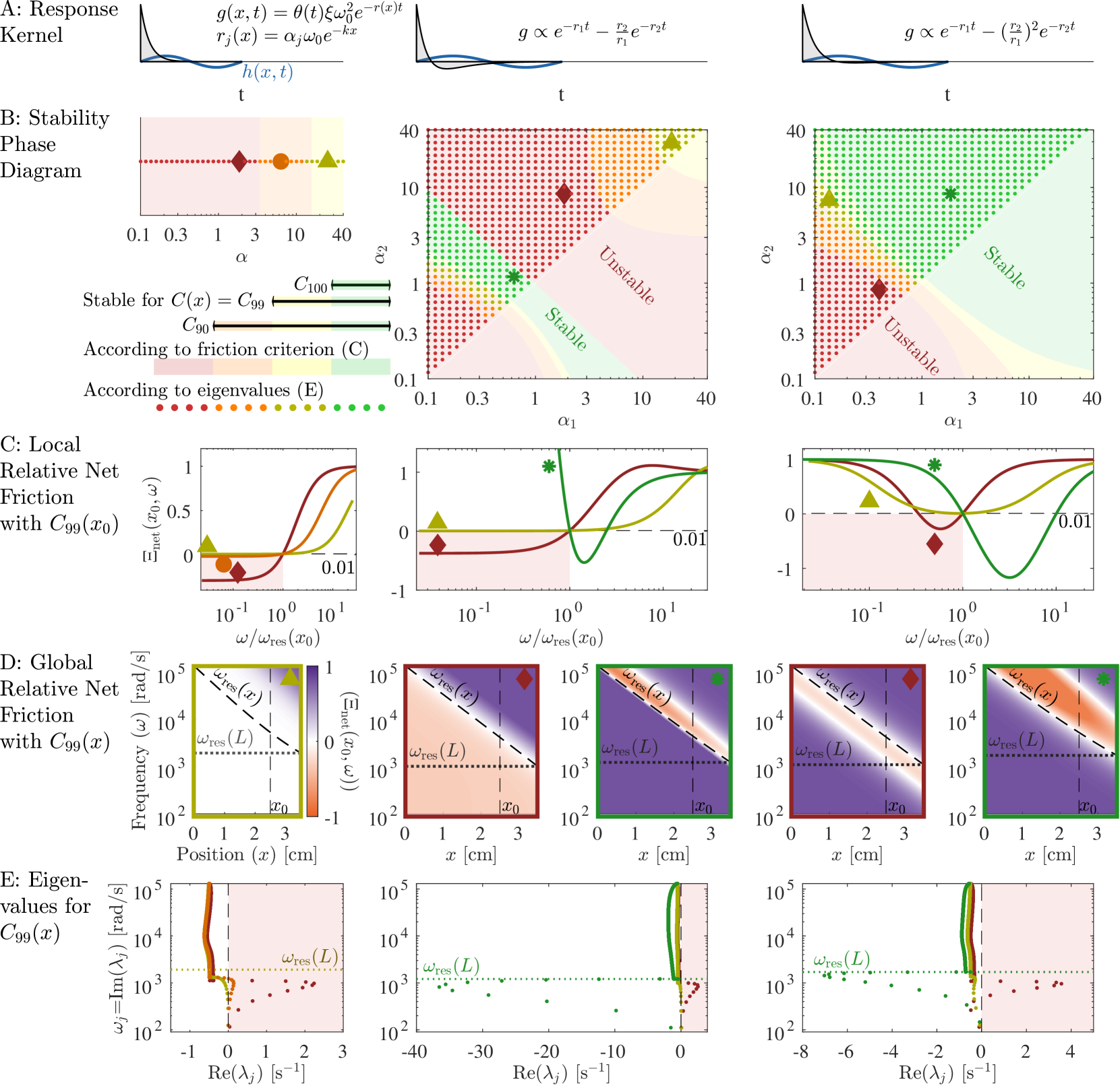
We propose a simple analytic condition that predicts whether the response kernel will destabilize the extended modes. Fixing some x=x0𝑥subscript𝑥0x=x_{0}italic_x = italic_x start_POSTSUBSCRIPT 0 end_POSTSUBSCRIPT, we ask whether there is any frequency 0ω<ωres(x0)0𝜔subscript𝜔ressubscript𝑥00\leq\omega<\omega_{\mathrm{res}}(x_{0})0 ≤ italic_ω < italic_ω start_POSTSUBSCRIPT roman_res end_POSTSUBSCRIPT ( italic_x start_POSTSUBSCRIPT 0 end_POSTSUBSCRIPT ) at which Im[Z(x0,ω)]<0𝑍subscript𝑥0𝜔0\imaginary[Z(x_{0},\omega)]<0start_OPERATOR roman_Im end_OPERATOR [ italic_Z ( italic_x start_POSTSUBSCRIPT 0 end_POSTSUBSCRIPT , italic_ω ) ] < 0. In that case, extended modes will experience some negative friction and may be unstable. Even though this simple criterion (shading in Fig. 3B) can be calculated without knowing the height eigenvectors or the coupling to the oval window, it predicts the stability of the extended modes (dots in Fig. 3B) well. (See Appendix G for a discussion of the oval window’s small effects.) In Fig. 3 we use this criterion, together with the stability obtained from calculating the eigenvalues via the Jacobian, to compare three different response kernels.

Single exponential kernel — So far we have used the response kernel introduced below Eq. 11, which integrates height for a time we assumed to be similar to the period of a wave resonant at that location:

g(x,Δt)𝑔𝑥Δ𝑡\displaystyle g(x,\Delta t)italic_g ( italic_x , roman_Δ italic_t ) =θ(Δt)ξω02er(x)Δt,r(x)=αωrespas(x)formulae-sequenceabsent𝜃Δ𝑡𝜉superscriptsubscript𝜔02superscript𝑒𝑟𝑥Δ𝑡𝑟𝑥𝛼superscriptsubscript𝜔respas𝑥\displaystyle=\theta(\Delta t)\>\xi\omega_{0}^{2}e^{-r(x)\Delta t},\quad r(x)=% \alpha\omega_{\mathrm{res}}^{\mathrm{pas}}(x)= italic_θ ( roman_Δ italic_t ) italic_ξ italic_ω start_POSTSUBSCRIPT 0 end_POSTSUBSCRIPT start_POSTSUPERSCRIPT 2 end_POSTSUPERSCRIPT italic_e start_POSTSUPERSCRIPT - italic_r ( italic_x ) roman_Δ italic_t end_POSTSUPERSCRIPT , italic_r ( italic_x ) = italic_α italic_ω start_POSTSUBSCRIPT roman_res end_POSTSUBSCRIPT start_POSTSUPERSCRIPT roman_pas end_POSTSUPERSCRIPT ( italic_x ) (15)
g~(x,ω)~𝑔𝑥𝜔\displaystyle\tilde{g}(x,\omega)over~ start_ARG italic_g end_ARG ( italic_x , italic_ω ) =ξω02r(x)iωr(x)2+ω2.absent𝜉superscriptsubscript𝜔02𝑟𝑥𝑖𝜔𝑟superscript𝑥2superscript𝜔2\displaystyle=\xi\omega_{0}^{2}\frac{r(x)-i\omega}{r(x)^{2}+\omega^{2}}.= italic_ξ italic_ω start_POSTSUBSCRIPT 0 end_POSTSUBSCRIPT start_POSTSUPERSCRIPT 2 end_POSTSUPERSCRIPT divide start_ARG italic_r ( italic_x ) - italic_i italic_ω end_ARG start_ARG italic_r ( italic_x ) start_POSTSUPERSCRIPT 2 end_POSTSUPERSCRIPT + italic_ω start_POSTSUPERSCRIPT 2 end_POSTSUPERSCRIPT end_ARG .

Here θ(Δt)𝜃Δ𝑡\theta(\Delta t)italic_θ ( roman_Δ italic_t ) is the Heaviside function that ensures a causal response. As we have seen in Fig. 2, for C(x)=C99(x)𝐶𝑥subscript𝐶99𝑥C(x)=C_{99}(x)italic_C ( italic_x ) = italic_C start_POSTSUBSCRIPT 99 end_POSTSUBSCRIPT ( italic_x ) and α=2𝛼2\alpha=2italic_α = 2 this choice leads to unstable extended modes since the net friction is negative everywhere for low frequencies. At the same time, the net friction is, by construction, slightly positive at the resonant frequency.

In Fig. 3C left we plot the relative net friction at a particular location x0subscript𝑥0x_{0}italic_x start_POSTSUBSCRIPT 0 end_POSTSUBSCRIPT for several values of α𝛼\alphaitalic_α. This Ξnet(x0,ω)subscriptΞnetsubscript𝑥0𝜔\Xi_{\mathrm{net}}(x_{0},\omega)roman_Ξ start_POSTSUBSCRIPT roman_net end_POSTSUBSCRIPT ( italic_x start_POSTSUBSCRIPT 0 end_POSTSUBSCRIPT , italic_ω ) is monotonically increasing as a function of frequency and is given by 1f1𝑓1-f1 - italic_f at resonance, by definition. Thus, as f𝑓fitalic_f approaches 1, net friction always becomes negative at lower frequencies, and hence our criterion predicts instability. In general, this criterion predicts stability only for αf/(1f)greater-than-or-equivalent-to𝛼𝑓1𝑓\alpha\gtrsim\sqrt{f/(1-f)}italic_α ≳ square-root start_ARG italic_f / ( 1 - italic_f ) end_ARG, in approximate agreement with our eigenvalue results (dots in Fig. 3B). Consequently, exponential kernels cannot bring localized modes to the edge of instability (f1𝑓1f\approx 1italic_f ≈ 1) without destabilizing extended modes, and thus we do not expect to find active processes with this form in hair cells. Can other response kernels stabilize these extended modes?

Approximate derivative kernel — The most common approach when studying cochlear dynamics is to assume friction is uniformly cancelled Julicher2003 ; hudspeth2010critique ; talmadge1998modeling , equivalent to taking a response kernel that implements an instantaneous derivative phc(x,t)th(x,t)proportional-tosubscript𝑝hc𝑥𝑡subscript𝑡𝑥𝑡p_{\mathrm{hc}}(x,t)\propto\partial_{t}h(x,t)italic_p start_POSTSUBSCRIPT roman_hc end_POSTSUBSCRIPT ( italic_x , italic_t ) ∝ ∂ start_POSTSUBSCRIPT italic_t end_POSTSUBSCRIPT italic_h ( italic_x , italic_t ) or g~(x,ω)iωproportional-to~𝑔𝑥𝜔𝑖𝜔\tilde{g}(x,\omega)\propto i\omegaover~ start_ARG italic_g end_ARG ( italic_x , italic_ω ) ∝ italic_i italic_ω. So if f1𝑓1f\leq 1italic_f ≤ 1, all modes at every position and frequency would experience a positive or zero relative net friction leading to stable extended modes. However, an instantaneous derivative requires an infinitely fast response of hair cells. With a finite response time, one can approximate a derivative by a sum of two exponentials:

g(x,Δt)=θ(Δt)ξω02[er1(x)Δtr2(x)r1(x)er2(x)Δt]𝑔𝑥Δ𝑡𝜃Δ𝑡𝜉superscriptsubscript𝜔02delimited-[]superscript𝑒subscript𝑟1𝑥Δ𝑡subscript𝑟2𝑥subscript𝑟1𝑥superscript𝑒subscript𝑟2𝑥Δ𝑡g(x,\Delta t)=\theta(\Delta t)\>\xi\omega_{0}^{2}\Big{[}e^{-r_{1}(x)\Delta t}-% \frac{r_{2}(x)}{r_{1}(x)}e^{-r_{2}(x)\Delta t}\Big{]}italic_g ( italic_x , roman_Δ italic_t ) = italic_θ ( roman_Δ italic_t ) italic_ξ italic_ω start_POSTSUBSCRIPT 0 end_POSTSUBSCRIPT start_POSTSUPERSCRIPT 2 end_POSTSUPERSCRIPT [ italic_e start_POSTSUPERSCRIPT - italic_r start_POSTSUBSCRIPT 1 end_POSTSUBSCRIPT ( italic_x ) roman_Δ italic_t end_POSTSUPERSCRIPT - divide start_ARG italic_r start_POSTSUBSCRIPT 2 end_POSTSUBSCRIPT ( italic_x ) end_ARG start_ARG italic_r start_POSTSUBSCRIPT 1 end_POSTSUBSCRIPT ( italic_x ) end_ARG italic_e start_POSTSUPERSCRIPT - italic_r start_POSTSUBSCRIPT 2 end_POSTSUBSCRIPT ( italic_x ) roman_Δ italic_t end_POSTSUPERSCRIPT ] (16)

with rj(x)=αjωrespas(x)subscript𝑟𝑗𝑥subscript𝛼𝑗superscriptsubscript𝜔respas𝑥r_{j}(x)=\alpha_{j}\omega_{\mathrm{res}}^{\mathrm{pas}}(x)italic_r start_POSTSUBSCRIPT italic_j end_POSTSUBSCRIPT ( italic_x ) = italic_α start_POSTSUBSCRIPT italic_j end_POSTSUBSCRIPT italic_ω start_POSTSUBSCRIPT roman_res end_POSTSUBSCRIPT start_POSTSUPERSCRIPT roman_pas end_POSTSUPERSCRIPT ( italic_x ). The relative coefficient r2/r1subscript𝑟2subscript𝑟1{-}r_{2}/r_{1}- italic_r start_POSTSUBSCRIPT 2 end_POSTSUBSCRIPT / italic_r start_POSTSUBSCRIPT 1 end_POSTSUBSCRIPT between the two terms ensures that 𝑑Δtg(x,Δt)=0differential-dΔ𝑡𝑔𝑥Δ𝑡0\int d\Delta t\>g(x,\Delta t)=0∫ italic_d roman_Δ italic_t italic_g ( italic_x , roman_Δ italic_t ) = 0, so that a time-independent shift in hhitalic_h has no effect on the response. In the limit α1,α2subscript𝛼1subscript𝛼2\alpha_{1},\alpha_{2}\rightarrow\inftyitalic_α start_POSTSUBSCRIPT 1 end_POSTSUBSCRIPT , italic_α start_POSTSUBSCRIPT 2 end_POSTSUBSCRIPT → ∞, this response kernel approaches an instantaneous derivative.

Figure 3B middle shows the stability phase diagram for this response kernel as a function of α1subscript𝛼1\alpha_{1}italic_α start_POSTSUBSCRIPT 1 end_POSTSUBSCRIPT and α2subscript𝛼2\alpha_{2}italic_α start_POSTSUBSCRIPT 2 end_POSTSUBSCRIPT. For f<1𝑓1f<1italic_f < 1, the extended modes are stabilized for large α𝛼\alphaitalic_α as in the case of a single exponential. But there is also a narrow range with α1α21less-than-or-similar-tosubscript𝛼1subscript𝛼21\alpha_{1}\alpha_{2}\lesssim 1italic_α start_POSTSUBSCRIPT 1 end_POSTSUBSCRIPT italic_α start_POSTSUBSCRIPT 2 end_POSTSUBSCRIPT ≲ 1 (green in Fig. 3B) where the extended modes can be stable all the way to f=1𝑓1f=1italic_f = 1. This true stability occurs because relative net friction has a negative slope at the resonance (green in Fig. 3C), so that negative net friction occurs at frequencies higher than resonance (orange in Fig. 3C). Perhaps surprisingly, this region of true stability occurs for low rates, α1α21less-than-or-similar-tosubscript𝛼1subscript𝛼21\alpha_{1}\alpha_{2}\lesssim 1italic_α start_POSTSUBSCRIPT 1 end_POSTSUBSCRIPT italic_α start_POSTSUBSCRIPT 2 end_POSTSUBSCRIPT ≲ 1. Hence, hair cells could implement kernels with this form, but not in the regime where they closely approximate an instantaneous derivative.

Zero-derivative kernel — Based on our simple condition for stability, can we construct a response kernel that leads to stable extended modes for a broader range of parameters? Since the simple analytic condition focuses on the behaviour of Ξnet(x,ω)subscriptΞnet𝑥𝜔\Xi_{\mathrm{net}}(x,\omega)roman_Ξ start_POSTSUBSCRIPT roman_net end_POSTSUBSCRIPT ( italic_x , italic_ω ) at low frequencies, we approximate it by a Taylor series in ω𝜔\omegaitalic_ω:

Ξnet(x,ω)=1+C(x)ξIm[ωg~|ω=0]+𝒪(ω).subscriptΞnet𝑥𝜔1𝐶𝑥𝜉evaluated-atsubscript𝜔~𝑔𝜔0𝒪𝜔\Xi_{\mathrm{net}}(x,\omega)=1+\frac{C(x)}{\xi}\imaginary[\left.\partial_{% \omega}\tilde{g}\right|_{\omega=0}]+\mathcal{O}(\omega).roman_Ξ start_POSTSUBSCRIPT roman_net end_POSTSUBSCRIPT ( italic_x , italic_ω ) = 1 + divide start_ARG italic_C ( italic_x ) end_ARG start_ARG italic_ξ end_ARG start_OPERATOR roman_Im end_OPERATOR [ ∂ start_POSTSUBSCRIPT italic_ω end_POSTSUBSCRIPT over~ start_ARG italic_g end_ARG | start_POSTSUBSCRIPT italic_ω = 0 end_POSTSUBSCRIPT ] + caligraphic_O ( italic_ω ) . (17)

A simple condition for positive net friction for small ω𝜔\omegaitalic_ω independent of C(x)𝐶𝑥C(x)italic_C ( italic_x ) is thus given by ωg~|ω=0=0evaluated-atsubscript𝜔~𝑔𝜔00\left.\partial_{\omega}\tilde{g}\right|_{\omega=0}=0∂ start_POSTSUBSCRIPT italic_ω end_POSTSUBSCRIPT over~ start_ARG italic_g end_ARG | start_POSTSUBSCRIPT italic_ω = 0 end_POSTSUBSCRIPT = 0, which in the time domain reads 0𝑑Δtg(x,Δt)Δt=0superscriptsubscript0differential-dΔ𝑡𝑔𝑥Δ𝑡Δ𝑡0\int_{0}^{\infty}d\Delta t\ g(x,\Delta t)\Delta t=0∫ start_POSTSUBSCRIPT 0 end_POSTSUBSCRIPT start_POSTSUPERSCRIPT ∞ end_POSTSUPERSCRIPT italic_d roman_Δ italic_t italic_g ( italic_x , roman_Δ italic_t ) roman_Δ italic_t = 0. This condition can be met by a sum of two exponentials weighted as follows:

g(x,Δt)=θ(Δt)ξω02[er1(x)Δtr2(x)2r1(x)2er2(x)Δt],𝑔𝑥Δ𝑡𝜃Δ𝑡𝜉superscriptsubscript𝜔02delimited-[]superscript𝑒subscript𝑟1𝑥Δ𝑡subscript𝑟2superscript𝑥2subscript𝑟1superscript𝑥2superscript𝑒subscript𝑟2𝑥Δ𝑡g(x,\Delta t)=\theta(\Delta t)\>\xi\omega_{0}^{2}\Big{[}e^{-r_{1}(x)\Delta t}-% \frac{r_{2}(x)^{2}}{r_{1}(x)^{2}}e^{-r_{2}(x)\Delta t}\Big{]},italic_g ( italic_x , roman_Δ italic_t ) = italic_θ ( roman_Δ italic_t ) italic_ξ italic_ω start_POSTSUBSCRIPT 0 end_POSTSUBSCRIPT start_POSTSUPERSCRIPT 2 end_POSTSUPERSCRIPT [ italic_e start_POSTSUPERSCRIPT - italic_r start_POSTSUBSCRIPT 1 end_POSTSUBSCRIPT ( italic_x ) roman_Δ italic_t end_POSTSUPERSCRIPT - divide start_ARG italic_r start_POSTSUBSCRIPT 2 end_POSTSUBSCRIPT ( italic_x ) start_POSTSUPERSCRIPT 2 end_POSTSUPERSCRIPT end_ARG start_ARG italic_r start_POSTSUBSCRIPT 1 end_POSTSUBSCRIPT ( italic_x ) start_POSTSUPERSCRIPT 2 end_POSTSUPERSCRIPT end_ARG italic_e start_POSTSUPERSCRIPT - italic_r start_POSTSUBSCRIPT 2 end_POSTSUBSCRIPT ( italic_x ) roman_Δ italic_t end_POSTSUPERSCRIPT ] , (18)

where rj(x)=αjωrespas(x)subscript𝑟𝑗𝑥subscript𝛼𝑗superscriptsubscript𝜔respas𝑥r_{j}(x)=\alpha_{j}\omega_{\mathrm{res}}^{\mathrm{pas}}(x)italic_r start_POSTSUBSCRIPT italic_j end_POSTSUBSCRIPT ( italic_x ) = italic_α start_POSTSUBSCRIPT italic_j end_POSTSUBSCRIPT italic_ω start_POSTSUBSCRIPT roman_res end_POSTSUBSCRIPT start_POSTSUPERSCRIPT roman_pas end_POSTSUPERSCRIPT ( italic_x ) as before. With this kernel, Fig. 3 right, there are three possible cases: In the first case, friction is positive everywhere. This case is only possible for f<1𝑓1f<1italic_f < 1 and gives rise to the yellow and orange area in the stability phase diagram. In the second case, friction is negative in a band of frequencies below the resonance frequency, leading to instability of the extended modes, see red area in Fig. 3B right. Finally, friction is positive below the resonant frequency but negative for a band of frequencies above the resonance frequency (green area). Importantly, this stable regime occurs for points α1α21greater-than-or-equivalent-tosubscript𝛼1subscript𝛼21\alpha_{1}\alpha_{2}\gtrsim 1italic_α start_POSTSUBSCRIPT 1 end_POSTSUBSCRIPT italic_α start_POSTSUBSCRIPT 2 end_POSTSUBSCRIPT ≳ 1 and therefore does not require much tuning of parameters.

Taken together, our results suggest that the extended modes are unstable if the net friction is negative for (a band of) frequencies lower than the resonance frequency. In principle, there are two ways to avoid this situation: either net friction is positive everywhere, or it is negative for a band of frequencies larger than the resonance frequency. The former can only occur if the net friction at resonance isn’t fully cancelled (f<1𝑓1f<1italic_f < 1), thus making this regime less useful for tuning the localized modes to the edge of instability. The latter regime also works for fully cancelled friction f=1𝑓1f=1italic_f = 1. It only occurs in a narrow parameter regime if the kernel approximates a derivative (Fig. 3 middle) but can be greatly enhanced if the kernel g~~𝑔\tilde{g}over~ start_ARG italic_g end_ARG instead exhibits a zero first derivative at ω=0𝜔0\omega=0italic_ω = 0 (Fig. 3 right). It is worth noting that for all forms of the kernel g~(x,ω)~𝑔𝑥𝜔\tilde{g}(x,\omega)over~ start_ARG italic_g end_ARG ( italic_x , italic_ω ) considered here, localized modes are at least marginally stable for all f1𝑓1f\leq 1italic_f ≤ 1.

Independent tuning of localized modes

Having established conditions on the stability of extended modes, we now turn to how hair cells can tune all localized modes to the edge of instability.
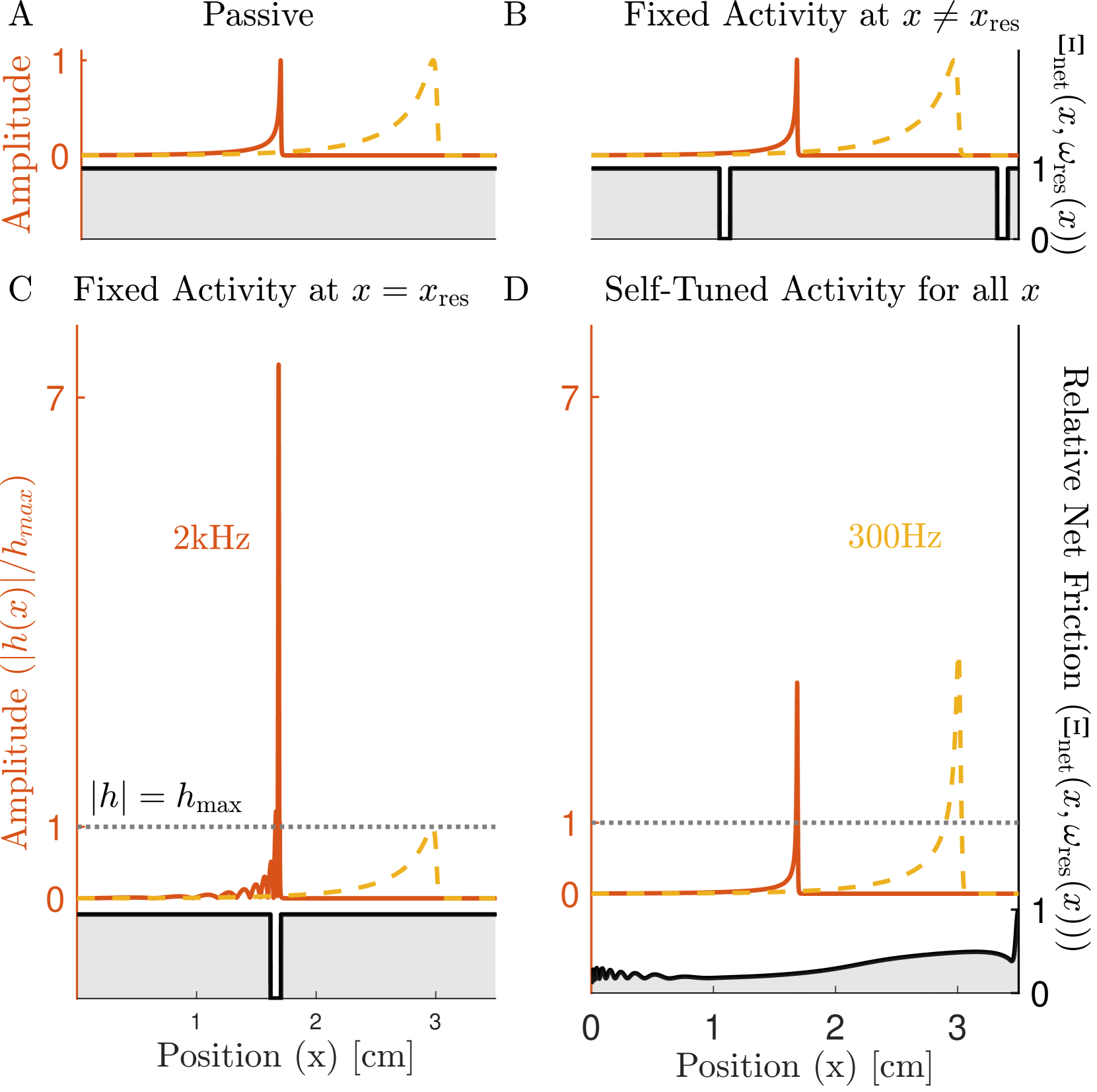
Refer to caption
Figure 4: Canceling friction has a predominantly local effect. We show the amplitude of the cochlea’s response to pure tones at 2000200020002000 Hz (orange) and 300300300300 Hz (yellow) for (A) a passive cochlea, C(x)=0𝐶𝑥0C(x)=0italic_C ( italic_x ) = 0, which by definition has Ξnet(x,ω)=1subscriptΞnet𝑥𝜔1\Xi_{\mathrm{net}}(x,\omega)=1roman_Ξ start_POSTSUBSCRIPT roman_net end_POSTSUBSCRIPT ( italic_x , italic_ω ) = 1, (B) friction reduced off-resonance, (C) friction reduced at the resonant position for 2000200020002000 Hz, giving an over 7-fold amplification, and (D) a cochlea self-tuned using Eq. 19, with target RMS height ten times greater than the passive one at each point, h0(x)=10h(x,t)2η|C=0subscript0𝑥evaluated-at10subscriptdelimited-⟨⟩superscript𝑥𝑡2𝜂𝐶0h_{0}(x)=10\left.\sqrt{\left\langle h(x,t)^{2}\right\rangle_{\eta}}\right|_{C=0}italic_h start_POSTSUBSCRIPT 0 end_POSTSUBSCRIPT ( italic_x ) = 10 square-root start_ARG ⟨ italic_h ( italic_x , italic_t ) start_POSTSUPERSCRIPT 2 end_POSTSUPERSCRIPT ⟩ start_POSTSUBSCRIPT italic_η end_POSTSUBSCRIPT end_ARG | start_POSTSUBSCRIPT italic_C = 0 end_POSTSUBSCRIPT. The left axis shows the amplitude of the response, normalized to peak at 1 in the passive case. The right axis shows the net effective friction at resonance Ξnet(x,ωres(x))subscriptΞnet𝑥subscript𝜔res𝑥\Xi_{\mathrm{net}}(x,\omega_{\mathrm{res}}(x))roman_Ξ start_POSTSUBSCRIPT roman_net end_POSTSUBSCRIPT ( italic_x , italic_ω start_POSTSUBSCRIPT roman_res end_POSTSUBSCRIPT ( italic_x ) ), Eq. 14, shown in gray in all panels.

Since the friction term in Zpassubscript𝑍pasZ_{\text{pas}}italic_Z start_POSTSUBSCRIPT pas end_POSTSUBSCRIPT is small compared to the canceling real parts, the relatively small absolute contribution of Zhcsubscript𝑍hcZ_{\text{hc}}italic_Z start_POSTSUBSCRIPT hc end_POSTSUBSCRIPT will dramatically affect mechanics only where the real part of Z𝑍Zitalic_Z is near 0. As a result, for kernels with stable extended modes, we propose that hair cells only need to cancel friction for the localized mode peaking at their location. Fig. 4 shows that if we reduce friction to near zero at a specific location, we only see a noticeable amplification of frequency modes that peak near that position (Fig. 4C). Off-resonance amplification (Fig. 4B) looks qualitatively identical to a passive system (Fig. 4A). Tuning the cochlea therefore only requires that friction is cancelled very near the resonant frequency (Im[Z(x,ωres(x))]=0𝑍𝑥subscript𝜔res𝑥0\imaginary[Z(x,\omega_{\mathrm{res}}(x))]=0start_OPERATOR roman_Im end_OPERATOR [ italic_Z ( italic_x , italic_ω start_POSTSUBSCRIPT roman_res end_POSTSUBSCRIPT ( italic_x ) ) ] = 0 for all x𝑥xitalic_x), a far less stringent limitation than globally nullifying friction (Im[Z(x,ω)]=0𝑍𝑥𝜔0\imaginary[Z(x,\omega)]=0start_OPERATOR roman_Im end_OPERATOR [ italic_Z ( italic_x , italic_ω ) ] = 0 for all x,ω𝑥𝜔x,\omegaitalic_x , italic_ω).

Self-tuning of active process strength

So far, we have shown that requiring stability of extended modes puts constraints on viable active hair cell responses and that for stable kernel choices all localized modes can be brought to the edge of instability simultaneously. In part this tuning is possible because the effects of C(x)𝐶𝑥C(x)italic_C ( italic_x ) are local both in space and in frequency. However, for strong amplification, it also requires the local hair cell activity strengths C(x)𝐶𝑥C(x)italic_C ( italic_x ) to be tuned very close to C100(x)subscript𝐶100𝑥C_{100}(x)italic_C start_POSTSUBSCRIPT 100 end_POSTSUBSCRIPT ( italic_x ), Fig. 5B. So, how can hair cells find the region where the net friction is cancelled (almost) perfectly along the line of resonant frequencies and thereby bring the set of localized modes to the proximity of their individual instabilities? Inspired by how isolated hair cells in non-mammalian vertebrates as, for example, bullfrogs can tune themselves to their Hopf bifurcation camalet2000auditory , cells could take advantage of the extreme sensitivity of the membrane displacement amplitude near C100(x)subscript𝐶100𝑥C_{100}(x)italic_C start_POSTSUBSCRIPT 100 end_POSTSUBSCRIPT ( italic_x ) to indirectly tune to this region, by measuring the amplitude of local displacements. This indirect tuning works much more robustly than tuning C(x)𝐶𝑥C(x)italic_C ( italic_x ) directly because the size of local oscillations in BM height are an order parameter for a dynamical bifurcation where C(x)𝐶𝑥C(x)italic_C ( italic_x ) is a control parameter.

Refer to caption
Figure 5: Self-tuning of active processes via feedback from the order parameter (RMS height) onto the control parameter (active process strength). (A) A sketch of how hair cell activity is tuned to counteract friction. At positions where hair cells experience a root-mean-square height below the threshold h0subscript0h_{0}italic_h start_POSTSUBSCRIPT 0 end_POSTSUBSCRIPT (dashed line), they slowly increase their activity, reducing the effective friction via Eq. 19, and vice versa. (B) Robust tuning of hair cell activity to the critical point. At a fixed position x0subscript𝑥0x_{0}italic_x start_POSTSUBSCRIPT 0 end_POSTSUBSCRIPT, we plot RMS height as a function of the activity strength C(x0)𝐶subscript𝑥0C(x_{0})italic_C ( italic_x start_POSTSUBSCRIPT 0 end_POSTSUBSCRIPT ) at that position. For simplicity, here we use the instantaneous derivative kernel g~(x,ω)=iξω~𝑔𝑥𝜔𝑖𝜉𝜔\tilde{g}(x,\omega)=-i\xi\omegaover~ start_ARG italic_g end_ARG ( italic_x , italic_ω ) = - italic_i italic_ξ italic_ω for which friction is fully cancelled when C(x)=1𝐶𝑥1C(x)=1italic_C ( italic_x ) = 1. We show how a 3% change in the activity strength C(x0)𝐶subscript𝑥0C(x_{0})italic_C ( italic_x start_POSTSUBSCRIPT 0 end_POSTSUBSCRIPT ) corresponds to a much larger relative change in the RMS height. Thus, while controlling C(x0)𝐶subscript𝑥0C(x_{0})italic_C ( italic_x start_POSTSUBSCRIPT 0 end_POSTSUBSCRIPT ) directly would require fine-tuning (red-shaded area), feedback based on the height only requires h0subscript0h_{0}italic_h start_POSTSUBSCRIPT 0 end_POSTSUBSCRIPT to fall on the steep part of this curve (green-shaded area). The region to the right of C(x0)=1𝐶subscript𝑥01C(x_{0})=1italic_C ( italic_x start_POSTSUBSCRIPT 0 end_POSTSUBSCRIPT ) = 1 is unstable.

We therefore consider feedback which, rather than directly implementing C(x)C100(x)𝐶𝑥subscript𝐶100𝑥C(x)\approx C_{100}(x)italic_C ( italic_x ) ≈ italic_C start_POSTSUBSCRIPT 100 end_POSTSUBSCRIPT ( italic_x ), instead adjusts C(x)𝐶𝑥C(x)italic_C ( italic_x ) to target an order parameter, the RMS displacement: h(x,t)2h0(x)expectation-valuesuperscript𝑥𝑡2subscript0𝑥\sqrt{\expectationvalue{h(x,t)^{2}}}\approx h_{0}(x)square-root start_ARG ⟨ start_ARG italic_h ( italic_x , italic_t ) start_POSTSUPERSCRIPT 2 end_POSTSUPERSCRIPT end_ARG ⟩ end_ARG ≈ italic_h start_POSTSUBSCRIPT 0 end_POSTSUBSCRIPT ( italic_x ). Because the effect of C(x)𝐶𝑥C(x)italic_C ( italic_x ) is predominantly local in x𝑥xitalic_x (Fig. 4), this can be implemented by local feedback (Fig. 5A). Thus we consider adding additional slow dynamics to the model:

τadC(x)dt=1h(x,t)2η(t)h0(x)2.subscript𝜏𝑎𝑑𝐶𝑥𝑑𝑡1subscriptexpectation-valuesuperscript𝑥𝑡2𝜂𝑡subscript0superscript𝑥2\tau_{a}\frac{dC(x)}{dt}=1-\frac{\expectationvalue{h(x,t)^{2}}_{\eta(t)}}{h_{0% }(x)^{2}}.italic_τ start_POSTSUBSCRIPT italic_a end_POSTSUBSCRIPT divide start_ARG italic_d italic_C ( italic_x ) end_ARG start_ARG italic_d italic_t end_ARG = 1 - divide start_ARG ⟨ start_ARG italic_h ( italic_x , italic_t ) start_POSTSUPERSCRIPT 2 end_POSTSUPERSCRIPT end_ARG ⟩ start_POSTSUBSCRIPT italic_η ( italic_t ) end_POSTSUBSCRIPT end_ARG start_ARG italic_h start_POSTSUBSCRIPT 0 end_POSTSUBSCRIPT ( italic_x ) start_POSTSUPERSCRIPT 2 end_POSTSUPERSCRIPT end_ARG . (19)

Here we assume that the timescale of the feedback τasubscript𝜏𝑎\tau_{a}italic_τ start_POSTSUBSCRIPT italic_a end_POSTSUBSCRIPT is much longer than the longest timescale of the sound-driven dynamics: τamuch-greater-thansubscript𝜏𝑎absent\tau_{a}\ggitalic_τ start_POSTSUBSCRIPT italic_a end_POSTSUBSCRIPT ≫1/20Hz. And we imagine that the system is externally driven by input from the ear canal, and model incoming sound as uncorrelated Gaussian noise in pressure: Pec(t)=η(t)subscript𝑃ec𝑡𝜂𝑡P_{\mathrm{ec}}(t)=\eta(t)italic_P start_POSTSUBSCRIPT roman_ec end_POSTSUBSCRIPT ( italic_t ) = italic_η ( italic_t ). Details of the noise spectrum do not qualitatively change our results as long as there is support for all frequencies resonant on the BM (see Appendix H). The temporal average needed for RMS displacement has thus been replaced by an average over this noise process — see Appendix B for details. (Due to symmetry, the average of h(x,t)𝑥𝑡h(x,t)italic_h ( italic_x , italic_t ) vanishes, h(x,t)η(t)=0subscriptdelimited-⟨⟩𝑥𝑡𝜂𝑡0\left\langle h(x,t)\right\rangle_{\eta(t)}=0⟨ italic_h ( italic_x , italic_t ) ⟩ start_POSTSUBSCRIPT italic_η ( italic_t ) end_POSTSUBSCRIPT = 0, thus feedback from the height squared is the first nonzero moment.) Fig. 6 shows the eigenvalue structure and the relative net friction Ξnet(x,ω)subscriptΞnet𝑥𝜔\Xi_{\mathrm{net}}(x,\omega)roman_Ξ start_POSTSUBSCRIPT roman_net end_POSTSUBSCRIPT ( italic_x , italic_ω ) of a cochlea tuned by this mechanism for a target RMS height h0(x)subscript0𝑥h_{0}(x)italic_h start_POSTSUBSCRIPT 0 end_POSTSUBSCRIPT ( italic_x ) set to be ten times the passive RMS height. We observe that, even in this case of a relatively small target RMS height h0subscript0h_{0}italic_h start_POSTSUBSCRIPT 0 end_POSTSUBSCRIPT, the real part of the eigenvalues is strongly reduced in magnitude, moving the localized modes considerably closer to the edge of instability.

Refer to caption
Figure 6: Effect of self-tuning via Eq. 19. (A) Eigenvalue structure of the passive (yellow) and the self-tuned system (green). Self-tuning moves all eigenvalues closer to instability. The localized modes near the end of the cochlea are less amplified, probably due to an interplay with the extended modes, which have most of their weight near the end of the cochlea, and boundary effects from the helicotrema. Note also the presence of extended modes even in the passive system. (B) Relative net friction Ξnet(x,ω)=ImZ(x,ω)/ξωsubscriptΞnet𝑥𝜔𝑍𝑥𝜔𝜉𝜔\Xi_{\mathrm{net}}(x,\omega)=\imaginary Z(x,\omega)/\xi\omegaroman_Ξ start_POSTSUBSCRIPT roman_net end_POSTSUBSCRIPT ( italic_x , italic_ω ) = start_OPERATOR roman_Im end_OPERATOR italic_Z ( italic_x , italic_ω ) / italic_ξ italic_ω after self-tuning. We note the slightly negative friction after resonance, similar to what is observed in the stable (green) case in Fig. 3D right. These plots use the zero-derivative kernel, Eq. 18, with α1=1,α2=2formulae-sequencesubscript𝛼11subscript𝛼22\alpha_{1}=1,\alpha_{2}=2italic_α start_POSTSUBSCRIPT 1 end_POSTSUBSCRIPT = 1 , italic_α start_POSTSUBSCRIPT 2 end_POSTSUBSCRIPT = 2. The target h0(x)subscript0𝑥h_{0}(x)italic_h start_POSTSUBSCRIPT 0 end_POSTSUBSCRIPT ( italic_x ) has been set to be ten times the passive RMS height as in Fig. 4D.

More generally, this scheme can bring each mode to the edge of instability without fine-tuning any fixed parameters (green in Fig. 5) since C(x)𝐶𝑥C(x)italic_C ( italic_x ) is a dynamical function approaching a steady-state value that only weakly depends on h0subscript0h_{0}italic_h start_POSTSUBSCRIPT 0 end_POSTSUBSCRIPT. This robust tuning is reminiscent of systems that exhibit self-organized criticality sornette_critical_1992 ; sornette_mapping_1995 ; camalet2000auditory ; buendia2020feedback , where a slowly varying control parameter is tuned via feedback from a fast order parameter.

Robustness to perturbations

This section examines two possible sources of variability and how, despite them, the system can still find its critical point. First, we consider a case in which the middle 10% of the cochlea is forced to have zero activity. We observe that points away from this region still reach their critical points and that inactive points very close to the edges of inactivity can be partially amplified (Fig. 7A). This observation reinforces the local nature of these active processes, showing that only friction at a given position needs to be reduced to achieve amplification for that position’s resonant frequency.

Another important part of our model is the stiffness of the basilar membrane, whose position dependence determines the resonance position of the different frequencies. To check how robust self-tuning is to slight changes in the stiffness profile, we consider a system in which the stiffness of the BM is noisy, replacing ω02e2kxsuperscriptsubscript𝜔02superscript𝑒2𝑘𝑥\omega_{0}^{2}e^{-2kx}italic_ω start_POSTSUBSCRIPT 0 end_POSTSUBSCRIPT start_POSTSUPERSCRIPT 2 end_POSTSUPERSCRIPT italic_e start_POSTSUPERSCRIPT - 2 italic_k italic_x end_POSTSUPERSCRIPT with ω02e2kxn(1+0.01γ(xn))superscriptsubscript𝜔02superscript𝑒2𝑘subscript𝑥𝑛10.01𝛾subscript𝑥𝑛\omega_{0}^{2}e^{-2kx_{n}}(1+0.01\gamma(x_{n}))italic_ω start_POSTSUBSCRIPT 0 end_POSTSUBSCRIPT start_POSTSUPERSCRIPT 2 end_POSTSUPERSCRIPT italic_e start_POSTSUPERSCRIPT - 2 italic_k italic_x start_POSTSUBSCRIPT italic_n end_POSTSUBSCRIPT end_POSTSUPERSCRIPT ( 1 + 0.01 italic_γ ( italic_x start_POSTSUBSCRIPT italic_n end_POSTSUBSCRIPT ) ), where γ(xn)𝛾subscript𝑥𝑛\gamma(x_{n})italic_γ ( italic_x start_POSTSUBSCRIPT italic_n end_POSTSUBSCRIPT ) is iid standard Gaussian noise. Figure 7B shows the resulting steady-state mean-square height profile. We see that self-tuning still achieves similar average enhancement, demonstrating that the exact stiffness profile is not necessary for amplification in the cochlea. However, the resulting system is quite noisy. We believe that this noisiness is due to the fact that the stiffness no longer decreases monotonically everywhere. If, as a result, the real part of the impedance is negative already before resonance, the travelling wave is exponentially suppressed and decays rapidly there. In order to match the target RMS height, hair cells at this location try to overcompensate by considerably increasing their activity. The resulting increase in C(x)𝐶𝑥C(x)italic_C ( italic_x ), however, also affects neighboring points and leads to the large spikes seen in Fig. 7B.

Refer to caption
Figure 7: The cochlear self-tuning is robust to perturbations. Mean-square height for (A) a simulation in which the middle 10%percent1010\%10 % of cells are inactive, i.e. C(x)=0𝐶𝑥0C(x)=0italic_C ( italic_x ) = 0 for 0.45L<x<0.55L0.45𝐿𝑥0.55𝐿0.45L<x<0.55L0.45 italic_L < italic_x < 0.55 italic_L, (B) a simulation for which the exponentially decaying stiffness ω02e2kxsuperscriptsubscript𝜔02superscript𝑒2𝑘𝑥\omega_{0}^{2}e^{-2kx}italic_ω start_POSTSUBSCRIPT 0 end_POSTSUBSCRIPT start_POSTSUPERSCRIPT 2 end_POSTSUPERSCRIPT italic_e start_POSTSUPERSCRIPT - 2 italic_k italic_x end_POSTSUPERSCRIPT has multiplicative white noise with a standard deviation of 1%. For both plots the target h0(x)subscript0𝑥h_{0}(x)italic_h start_POSTSUBSCRIPT 0 end_POSTSUBSCRIPT ( italic_x ) is five times the passive RMS height. Note that we use a discretization scale of N=4000𝑁4000N=4000italic_N = 4000, which might not be large enough to resolve the peaks of the high-frequency localized modes close to x=0𝑥0x=0italic_x = 0 and lead to the observed spikes there in (A).

Discussion

The high sensitivity, dynamic range, and frequency resolution of human hearing are all thought to arise due to proximity of individual oscillators to Hopf bifurcations, driven by hair cell activity that effectively reduces friction hudspeth2010critique . Here we introduce a wave equation for the basilar membrane that includes hair cell activity in terms of a generic response kernel, with a position-dependent activity strength, and analyze its mode structure.

We find modes that peak at a resonant position, which we call localized modes, and argue that it is these modes whose Hopf bifurcations enable the fidelity of hearing. Although different spatial locations are, in principle, coupled by fluid flow and influenced by hair cell activity throughout the cochlea, we demonstrate that for small friction, the localized modes become so sharply peaked that different positions are nearly uncoupled. In this small friction limit the amplification of each mode is dependent only on the activity of hair cells near the resonant position. Thus, a simple, local feedback scheme for hair cell activity strength can tune all localized modes to the edge of instability.

Surprisingly, however, we also find a second set of modes, which we call extended modes. These are standing-wave-like, and couple to essentially all hair cells. The existence of these modes does not depend on hair cell activity and they are also present in our passive model. Indeed, we also find them in previous models neely1986model ; elliott2007state ; elliott2011erratum ; talmadge1993new , see Appendices C and  D. We show that requiring stability of extended modes provides strong limitations on viable hair cell responses. In particular, our results suggest that approximations to the derivative kernel, which is often implicitly assumed to underly hair cell activity Julicher2003 ; wang2019emergence , generically lead to unstable extended modes. Other kernels might be better suited, and we find criteria for the temporal shape of active processes which hair cells must obey. An interesting question for further research is to understand which proposed molecular mechanisms satisfy these criteria. For kernels which obey these criteria the localized modes become unstable at smaller activity strength than the extended modes do, and so local tuning can bring the localized modes independently to the edge of instability. In the self-organized steady-state of our model, effective friction is only cancelled along the one-dimensional resonant line through the two-dimensional space of frequency and cochlear position. This is in contrast to existing models that analyze a nonlinear cochlea by assuming that friction has been set globally to (near) zero Julicher2003 ; reichenbach2014physics ; talmadge1993new .

Models for isolated hair cells without a cochlea use a feedback scheme similar to ours, with a control parameter, usually calcium activity, tuned towards a Hopf bifurcation nadrowski2004active ; camalet2000auditory . In both cases, tuning is based on the (local) order parameter, here the BM displacement, and works robustly due to the large susceptibility at the critical point. Using criticality for sensing might indeed be common in biological systems. For instance, for E. coli chemosensing, we and others have proposed that cell receptor arrays tune themselves close to criticality to detect small changes in concentration keegstra2022near ; sherry2024lattice . In the neural realm, we have suggested that proximity to a bifurcation of the voltage dynamics might underly the incredible temperature sensitivity of pit vipers graf2023bifurcation and allow fruit flies to reliably extract odor timing information for navigation choi.etal_2024 . Furthermore, it is thought that the schooling behaviour of fish, flocking of birds and swarming of insects are near a phase transition to optimize collective computation bonabeau1997self ; niwa1994self ; romanczuk2023phase . Finally, it has been shown that an anti-Hebbian learning rule in neurons whose connectivity is suppressed in response to activity can lead to a self-organized dynamical critical state levina2007dynamical ; magnasco2009self ; landmann_self-organized_2021 .

Whether the order-parameter based feedback scheme presented here is implemented in hair cells could be tested by measuring the cochlea’s response when given a continuous signal at a limited frequency bandwidth. We expect hair cell activity at positions with a resonant frequency close to that of the signal to decrease while having a minimal effect for positions further away. Directly testing this prediction would require measuring the response in a live cochlea, a difficult but perhaps feasible task with emerging optical coherence tomography techniques vogl2022methods ; olson2020cochlear . It might also be possible to indirectly test this prediction with simpler psychoacoustic methods.

While our model provides a mechanism for the cochlea to tune itself using only local information, there are hints that there is at least some nonlocal feedback. Under contralateral stimulation (sound played in the opposite ear), the frequency of known otoacoustic emissions (OAEs) shifts. This phenomenon is thought to be due to changes in outer hair cell activity induced by signals from neurons in the MOC bundle lewis2020efferent . In our model, such shifts also occur naturally if contralateral stimulation globally decreases C(x)𝐶𝑥C(x)italic_C ( italic_x ): If the contribution Zhcsubscript𝑍hcZ_{\text{hc}}italic_Z start_POSTSUBSCRIPT hc end_POSTSUBSCRIPT of hair cells to the impedance is not purely imaginary, a change in C(x)𝐶𝑥C(x)italic_C ( italic_x ) shifts the resonant frequency of that position (and thereby changes the frequency of otoacoustic emissions) by a small amount ΔωΔCRe[g~]proportional-toΔ𝜔Δ𝐶~𝑔\Delta\omega\propto\Delta C\real[\tilde{g}]roman_Δ italic_ω ∝ roman_Δ italic_C start_OPERATOR roman_Re end_OPERATOR [ over~ start_ARG italic_g end_ARG ]. Such frequency shifts have indeed been observed in lizards koppl1993spontaneous . Should they also be observed in human hearing when stimulation happens in the same ear as the measurement of OAEs, this could lend further credence to our local order parameter-based feedback.

Early evidence for the importance of a Hopf bifurcation in hearing came from characteristic nonlinearities, including that the BM wave amplitude grows as the 1/3131/31 / 3 power of sound amplitude and a prominent third harmonic in evoked otoacoustic emissions reichenbach2014physics ; hudspeth2010critique ; Julicher2003 . Our model is explicitly linear, which we expect to be a good approximation far from the edge of instability. But when hair cell activity is strong enough to precisely bring the impedance at resonance to zero, the small nonlinearities of the basilar membrane become the dominant restoring force. It is thus an interesting question for future research how these nonlinearities interact with extended modes.

In addition to making a linear approximation, we discretized the cochlea to understand its mode structure. This discretization separates the BM into segments of length L/N𝐿𝑁L/Nitalic_L / italic_N where N𝑁Nitalic_N typically ranged from 1000 to 4000 in our numerics. The real cochlea also contains a small spatial scale, set by the length at which lateral coupling dominates, around 20μ20𝜇20\mu20 italic_μnaidu2001longitudinal ; emadi2004stiffness , corresponding to around 2000 independent segments. We expect that the number, shapes and eigenvalues of the extended modes will be independent of details at this small spatial scale. However, the details of the short length-scale physics might influence localized modes in interesting ways.

Frequency discrimination and signal amplification in the range of 20100020100020-100020 - 1000Hz remains an area of active research reichenbach2010ratchet . Since the extended modes exhibit resonant frequencies below the lowest resonant frequency of the basilar membrane (165165165165Hz), they could potentially contribute to the cochlea’s low-frequency sensitivity. Indeed, experimental measurements of BM dynamics have revealed a constant phase slope near the cochlear apex, indicating that low-frequency waves reach the helicotrema cooper1995nonlinear ; recio2017mechanical . This observation aligns with the characteristics of the extended modes we present and the exploration of these extended modes and their impact on hearing continues to be an exciting avenue for future research.

Acknowledgements.
We thank Jim Hudspeth and the members of the Machta group for helpful discussions, and Pranav Kantroo, Mason Rouches, Derek Sherry and Jose Betancourt for constructive comments on the manuscript. This work was supported by the Deutsche Forschungsgemeinschaft (DFG, German Research Foundation) Projektnummer 494077061 (IRG), and by NIH R35GM138341 (BBM) and a Simons Investigator award (BBM).

References

  • (1) T. Reichenbach and A. Hudspeth, “The physics of hearing: fluid mechanics and the active process of the inner ear,” Reports on Progress in Physics, vol. 77, no. 7, p. 076601, 2014.
  • (2) D. T. Kemp, “Evidence of mechanical nonlinearity and frequency selective wave amplification in the cochlea,” Archives of oto-rhino-laryngology, vol. 224, no. 1, pp. 37–45, 1979.
  • (3) P. Dallos, “The active cochlea,” Journal of Neuroscience, vol. 12, no. 12, pp. 4575–4585, 1992.
  • (4) P. Martin and A. Hudspeth, “Active hair-bundle movements can amplify a hair cell’s response to oscillatory mechanical stimuli,” Proceedings of the National Academy of Sciences, vol. 96, no. 25, pp. 14306–14311, 1999.
  • (5) T. Ren, W. He, and P. G. Gillespie, “Measurement of cochlear power gain in the sensitive gerbil ear,” Nature communications, vol. 2, no. 1, pp. 1–7, 2011.
  • (6) B. Nadrowski, P. Martin, and F. Jülicher, “Active hair-bundle motility harnesses noise to operate near an optimum of mechanosensitivity,” Proceedings of the National Academy of Sciences, vol. 101, no. 33, pp. 12195–12200, 2004.
  • (7) Y. Roongthumskul, L. Fredrickson-Hemsing, A. Kao, and D. Bozovic, “Multiple-timescale dynamics underlying spontaneous oscillations of saccular hair bundles,” Biophysical journal, vol. 101, no. 3, pp. 603–610, 2011.
  • (8) S. Camalet, T. Duke, F. Jülicher, and J. Prost, “Auditory sensitivity provided by self-tuned critical oscillations of hair cells,” Proceedings of the national academy of sciences, vol. 97, no. 7, pp. 3183–3188, 2000.
  • (9) R. A. Eatock, D. P. Corey, and A. Hudspeth, “Adaptation of mechanoelectrical transduction in hair cells of the bullfrog’s sacculus,” Journal of Neuroscience, vol. 7, no. 9, pp. 2821–2836, 1987.
  • (10) T. Duke and F. Jülicher, “Active traveling wave in the cochlea,” Phys. Rev. Lett., vol. 90, p. 158101, Apr 2003.
  • (11) J. Lighthill, “Energy flow in the cochlea,” Journal of fluid mechanics, vol. 106, pp. 149–213, 1981.
  • (12) C. Talmadge, G. Long, W. Murphy, and A. Tubis, “New off-line method for detecting spontaneous otoacoustic emissions in human subjects,” Hearing research, vol. 71, no. 1-2, pp. 170–182, 1993.
  • (13) V. M. Eguíluz, M. Ospeck, Y. Choe, A. Hudspeth, and M. O. Magnasco, “Essential nonlinearities in hearing,” Physical review letters, vol. 84, no. 22, p. 5232, 2000.
  • (14) C. L. Talmadge, A. Tubis, G. R. Long, and P. Piskorski, “Modeling otoacoustic emission and hearing threshold fine structures,” The Journal of the Acoustical Society of America, vol. 104, no. 3, pp. 1517–1543, 1998.
  • (15) D. Sornette, “Critical phase transitions made self-organized: a dynamical system feedback mechanism for self-organized criticality,” Journal de Physique I, vol. 2, no. 11, pp. 2065–2073, 1992.
  • (16) D. Sornette, A. Johansen, and I. Dornic, “Mapping self-organized criticality onto criticality,” Journal de Physique I, vol. 5, no. 3, pp. 325–335, 1995.
  • (17) G. Emadi, C.-P. Richter, and P. Dallos, “Stiffness of the gerbil basilar membrane: radial and longitudinal variations,” Journal of neurophysiology, vol. 91, no. 1, pp. 474–488, 2004.
  • (18) D. D. Greenwood, “A cochlear frequency-position function for several species—29 years later,” The Journal of the Acoustical Society of America, vol. 87, no. 6, pp. 2592–2605, 1990.
  • (19) P. Martin and A. Hudspeth, “Mechanical frequency tuning by sensory hair cells, the receptors and amplifiers of the inner ear,” Annual Review of Condensed Matter Physics, vol. 12, no. 1, 2021.
  • (20) K. Iwasa and M. Adachi, “Force generation in the outer hair cell of the cochlea,” Biophysical journal, vol. 73, no. 1, pp. 546–555, 1997.
  • (21) S. J. Elliott, E. M. Ku, and B. Lineton, “A state space model for cochlear mechanics,” The Journal of the Acoustical Society of America, vol. 122, no. 5, pp. 2759–2771, 2007.
  • (22) A. Hudspeth, F. Jülicher, and P. Martin, “A critique of the critical cochlea: Hopf—a bifurcation—is better than none,” Journal of neurophysiology, vol. 104, no. 3, pp. 1219–1229, 2010.
  • (23) S. T. Neely and D. Kim, “A model for active elements in cochlear biomechanics,” The journal of the acoustical society of America, vol. 79, no. 5, pp. 1472–1480, 1986.
  • (24) S. J. Elliott, E. M. Ku, and B. Lineton, “Erratum:“a state space model for cochlear mechanics”[j. acoust. soc. am. 122 (5), 2759–2771 (2007)],” The Journal of the Acoustical Society of America, vol. 130, no. 5, pp. 3158–3158, 2011.
  • (25) V. Buendía, S. Di Santo, J. A. Bonachela, and M. A. Muñoz, “Feedback mechanisms for self-organization to the edge of a phase transition,” Frontiers in Physics, vol. 8, p. 333, 2020.
  • (26) S.-W. Wang and L.-H. Tang, “Emergence of collective oscillations in adaptive cells,” Nature Communications, vol. 10, no. 1, p. 5613, 2019.
  • (27) J. M. Keegstra, F. Avgidis, Y. Mulla, J. S. Parkinson, and T. S. Shimizu, “Near-critical tuning of cooperativity revealed by spontaneous switching in a protein signalling array,” bioRxiv 2022.12.04.518992, 2022.
  • (28) D. M. Sherry, I. R. Graf, S. J. Bryant, T. Emonet, and B. B. Machta, “Lattice ultrasensitivity produces large gain in e. coli chemosensing,” arXiv:2405.18331, 2024.
  • (29) I. R. Graf and B. B. Machta, “A bifurcation integrates information from many noisy ion channels and allows for milli-kelvin thermal sensitivity in the snake pit organ,” Proceedings of the National Academy of Sciences, vol. 121, no. 6, p. e2308215121, 2024.
  • (30) K. Choi, W. Rosenbluth, I. R. Graf, N. Kadakia, and T. Emonet, “Bifurcation enhances temporal information encoding in the olfactory periphery,” PRX Life, vol. 2, p. 043011, Nov 2024.
  • (31) E. Bonabeau, G. Theraulaz, J.-L. Deneubourg, S. Aron, and S. Camazine, “Self-organization in social insects,” Trends in Ecology & Evolution, vol. 12, no. 5, pp. 188–193, 1997.
  • (32) H.-S. Niwa, “Self-organizing dynamic model of fish schooling,” Journal of theoretical Biology, vol. 171, no. 2, pp. 123–136, 1994.
  • (33) P. Romanczuk and B. C. Daniels, “Phase transitions and criticality in the collective behavior of animals—self-organization and biological function,” in Order, Disorder and Criticality: Advanced Problems of Phase Transition Theory, pp. 179–208, World Scientific, 2023.
  • (34) A. Levina, J. M. Herrmann, and T. Geisel, “Dynamical synapses causing self-organized criticality in neural networks,” Nature physics, vol. 3, no. 12, pp. 857–860, 2007.
  • (35) M. O. Magnasco, O. Piro, and G. A. Cecchi, “Self-tuned critical anti-hebbian networks,” Physical review letters, vol. 102, no. 25, p. 258102, 2009.
  • (36) S. Landmann, L. Baumgarten, and S. Bornholdt, “Self-organized criticality in neural networks from activity-based rewiring,” Physical Review E, vol. 103, no. 3, p. 032304, 2021.
  • (37) C. Vogl, J. Neef, and C. Wichmann, “Methods for multiscale structural and functional analysis of the mammalian cochlea,” Molecular and Cellular Neuroscience, vol. 120, p. 103720, 2022.
  • (38) E. S. Olson and C. E. Strimbu, “Cochlear mechanics: New insights from vibrometry and optical coherence tomography,” Current opinion in physiology, vol. 18, pp. 56–62, 2020.
  • (39) J. D. Lewis, “Efferent-induced shifts in synchronized-spontaneous-otoacoustic-emission magnitude and frequency,” The Journal of the Acoustical Society of America, vol. 148, no. 5, pp. 3258–3269, 2020.
  • (40) C. Köppl and G. A. Manley, “Spontaneous otoacoustic emissions in the bobtail lizard. i: General characteristics,” Hearing research, vol. 71, no. 1-2, pp. 157–169, 1993.
  • (41) R. C. Naidu and D. C. Mountain, “Longitudinal coupling in the basilar membrane,” JARO: Journal of the Association for Research in Otolaryngology, vol. 2, no. 3, p. 257, 2001.
  • (42) T. Reichenbach and A. Hudspeth, “A ratchet mechanism for amplification in low-frequency mammalian hearing,” Proceedings of the National Academy of Sciences, vol. 107, no. 11, pp. 4973–4978, 2010.
  • (43) N. P. Cooper and W. S. Rhode, “Nonlinear mechanics at the apex of the guinea-pig cochlea,” Hearing research, vol. 82, no. 2, pp. 225–243, 1995.
  • (44) A. Recio-Spinoso and J. S. Oghalai, “Mechanical tuning and amplification within the apex of the guinea pig cochlea,” The Journal of physiology, vol. 595, no. 13, pp. 4549–4561, 2017.
  • (45) T. Kis, “Tridiagonal matrix algorithm.” https://github.com/tamaskis/tridiagonal-MATLAB/releases/tag/v5.1.0 Retrieved December 12, 2024.

Appendices

The first two appendix sections show full details of how we write the discretized model in matrix form, and how we calculate the RMS height for self-tuning. The remaining sections are robustness checks of various kinds. They investigate the effect of altering parameters and the exact form of the response kernels in our model, and confirm that previous models exhibit similar behavior.

Appendix A.   Constructing the Jacobian J^bold-^𝐽\hat{J}overbold_^ start_ARG bold_italic_J end_ARG for linear response kernels

Our passive cochlear model is based on work from Ref. talmadge1998modeling , with a few changes in notation and any larger differences discussed in Appendix C. We model the cochlea with two compartments. First we consider the bulk of the cochlea where sound induces flux of water in the upper and lower compartment; we define j(x,t)=jlower(x,t)jupper(x,t)𝑗𝑥𝑡subscript𝑗lower𝑥𝑡subscript𝑗upper𝑥𝑡j(x,t)=j_{\text{lower}}(x,t)-j_{\text{upper}}(x,t)italic_j ( italic_x , italic_t ) = italic_j start_POSTSUBSCRIPT lower end_POSTSUBSCRIPT ( italic_x , italic_t ) - italic_j start_POSTSUBSCRIPT upper end_POSTSUBSCRIPT ( italic_x , italic_t ) as the difference in volume current between the scala tympani and scala vestibuli. According to force balance, this creates a corresponding pressure difference p(x,t)=plower(x,t)pupper(x,t)𝑝𝑥𝑡subscript𝑝lower𝑥𝑡subscript𝑝upper𝑥𝑡p(x,t)=p_{\text{lower}}(x,t)-p_{\text{upper}}(x,t)italic_p ( italic_x , italic_t ) = italic_p start_POSTSUBSCRIPT lower end_POSTSUBSCRIPT ( italic_x , italic_t ) - italic_p start_POSTSUBSCRIPT upper end_POSTSUBSCRIPT ( italic_x , italic_t ), between the two compartments,

ρtj(x,t)=Acsxp(x,t)𝜌subscript𝑡𝑗𝑥𝑡subscript𝐴cssubscript𝑥𝑝𝑥𝑡\rho\partial_{t}j(x,t)=-A_{\text{cs}}\partial_{x}p(x,t)italic_ρ ∂ start_POSTSUBSCRIPT italic_t end_POSTSUBSCRIPT italic_j ( italic_x , italic_t ) = - italic_A start_POSTSUBSCRIPT cs end_POSTSUBSCRIPT ∂ start_POSTSUBSCRIPT italic_x end_POSTSUBSCRIPT italic_p ( italic_x , italic_t ) (A1)

where Acssubscript𝐴csA_{\text{cs}}italic_A start_POSTSUBSCRIPT cs end_POSTSUBSCRIPT is the average cross-sectional area of a cochlear compartment and ρ𝜌\rhoitalic_ρ is the density of water. The fluid flux propagates down the cochlea, creating a displacement h(x,t)𝑥𝑡h(x,t)italic_h ( italic_x , italic_t ) of the BM, which we call height. The fluid flux obeys a continuity equation

2Wbmth(x,t)+xj(x,t)=0,2subscript𝑊bmsubscript𝑡𝑥𝑡subscript𝑥𝑗𝑥𝑡02W_{\text{bm}}\partial_{t}h(x,t)+\partial_{x}j(x,t)=0,2 italic_W start_POSTSUBSCRIPT bm end_POSTSUBSCRIPT ∂ start_POSTSUBSCRIPT italic_t end_POSTSUBSCRIPT italic_h ( italic_x , italic_t ) + ∂ start_POSTSUBSCRIPT italic_x end_POSTSUBSCRIPT italic_j ( italic_x , italic_t ) = 0 , (A2)

where Wbmsubscript𝑊bmW_{\text{bm}}italic_W start_POSTSUBSCRIPT bm end_POSTSUBSCRIPT is the width of the BM. We can eliminate j(x,t)𝑗𝑥𝑡j(x,t)italic_j ( italic_x , italic_t ) from Eq. A1 and A2 to arrive at a modified wave equation,

2ρWbmAcst2h(x,t)=x2p(x,t).2𝜌subscript𝑊bmsubscript𝐴cssuperscriptsubscript𝑡2𝑥𝑡superscriptsubscript𝑥2𝑝𝑥𝑡\frac{2\rho W_{\text{bm}}}{A_{\text{cs}}}\partial_{t}^{2}h(x,t)=\partial_{x}^{% 2}p(x,t).divide start_ARG 2 italic_ρ italic_W start_POSTSUBSCRIPT bm end_POSTSUBSCRIPT end_ARG start_ARG italic_A start_POSTSUBSCRIPT cs end_POSTSUBSCRIPT end_ARG ∂ start_POSTSUBSCRIPT italic_t end_POSTSUBSCRIPT start_POSTSUPERSCRIPT 2 end_POSTSUPERSCRIPT italic_h ( italic_x , italic_t ) = ∂ start_POSTSUBSCRIPT italic_x end_POSTSUBSCRIPT start_POSTSUPERSCRIPT 2 end_POSTSUPERSCRIPT italic_p ( italic_x , italic_t ) . (A3)

For our numerical solution, we use a finite element approximation to this equation where we break the cochlea into N𝑁Nitalic_N points separated by a distance δx=LN𝛿𝑥𝐿𝑁\delta x=\frac{L}{N}italic_δ italic_x = divide start_ARG italic_L end_ARG start_ARG italic_N end_ARG, and we label each point xn=nδxsubscript𝑥𝑛𝑛𝛿𝑥x_{n}=n\delta xitalic_x start_POSTSUBSCRIPT italic_n end_POSTSUBSCRIPT = italic_n italic_δ italic_x with n=1,2,,N𝑛12𝑁n=1,2,...,Nitalic_n = 1 , 2 , … , italic_N. Now Eq. A3 becomes,

2ρWbmAcst2h(xn,t)=x2p(xn,t)p(xn+1,t)2p(xn,t)+p(xn1,t)δx2.2𝜌subscript𝑊bmsubscript𝐴cssuperscriptsubscript𝑡2subscript𝑥𝑛𝑡superscriptsubscript𝑥2𝑝subscript𝑥𝑛𝑡𝑝subscript𝑥𝑛1𝑡2𝑝subscript𝑥𝑛𝑡𝑝subscript𝑥𝑛1𝑡𝛿superscript𝑥2\frac{2\rho W_{\text{bm}}}{A_{\text{cs}}}\partial_{t}^{2}h(x_{n},t)=\partial_{% x}^{2}p(x_{n},t)\approx\frac{p(x_{n+1},t)-2p(x_{n},t)+p(x_{n-1},t)}{\delta x^{% 2}}.divide start_ARG 2 italic_ρ italic_W start_POSTSUBSCRIPT bm end_POSTSUBSCRIPT end_ARG start_ARG italic_A start_POSTSUBSCRIPT cs end_POSTSUBSCRIPT end_ARG ∂ start_POSTSUBSCRIPT italic_t end_POSTSUBSCRIPT start_POSTSUPERSCRIPT 2 end_POSTSUPERSCRIPT italic_h ( italic_x start_POSTSUBSCRIPT italic_n end_POSTSUBSCRIPT , italic_t ) = ∂ start_POSTSUBSCRIPT italic_x end_POSTSUBSCRIPT start_POSTSUPERSCRIPT 2 end_POSTSUPERSCRIPT italic_p ( italic_x start_POSTSUBSCRIPT italic_n end_POSTSUBSCRIPT , italic_t ) ≈ divide start_ARG italic_p ( italic_x start_POSTSUBSCRIPT italic_n + 1 end_POSTSUBSCRIPT , italic_t ) - 2 italic_p ( italic_x start_POSTSUBSCRIPT italic_n end_POSTSUBSCRIPT , italic_t ) + italic_p ( italic_x start_POSTSUBSCRIPT italic_n - 1 end_POSTSUBSCRIPT , italic_t ) end_ARG start_ARG italic_δ italic_x start_POSTSUPERSCRIPT 2 end_POSTSUPERSCRIPT end_ARG . (A4)

We now turn our attention to the boundary conditions. At the left-hand side, we have a Neumann boundary condition where the lateral displacement of the oval window dow(t)subscript𝑑ow𝑡d_{\mathrm{ow}}(t)italic_d start_POSTSUBSCRIPT roman_ow end_POSTSUBSCRIPT ( italic_t ) creates a flux of fluid, which propagates down the cochlea and induces an equal but opposite flux at the round window, due to fluid incompressibility. Via Eq. A1, this flux leads to a pressure gradient:

t2dow(t)Acs2ρAowp(x1,t)p(0,t)δxsuperscriptsubscript𝑡2subscript𝑑ow𝑡subscript𝐴cs2𝜌subscript𝐴ow𝑝subscript𝑥1𝑡𝑝0𝑡𝛿𝑥\partial_{t}^{2}{d}_{\text{ow}}(t)\approx\frac{A_{\text{cs}}}{2\rho A_{\text{% ow}}}\frac{p(x_{1},t)-p(0,t)}{\delta x}∂ start_POSTSUBSCRIPT italic_t end_POSTSUBSCRIPT start_POSTSUPERSCRIPT 2 end_POSTSUPERSCRIPT italic_d start_POSTSUBSCRIPT ow end_POSTSUBSCRIPT ( italic_t ) ≈ divide start_ARG italic_A start_POSTSUBSCRIPT cs end_POSTSUBSCRIPT end_ARG start_ARG 2 italic_ρ italic_A start_POSTSUBSCRIPT ow end_POSTSUBSCRIPT end_ARG divide start_ARG italic_p ( italic_x start_POSTSUBSCRIPT 1 end_POSTSUBSCRIPT , italic_t ) - italic_p ( 0 , italic_t ) end_ARG start_ARG italic_δ italic_x end_ARG (A5)

where Aowsubscript𝐴owA_{\mathrm{ow}}italic_A start_POSTSUBSCRIPT roman_ow end_POSTSUBSCRIPT is the area of the oval window. The oval window itself acts as a damped harmonic oscillator:

t2dow(t)+ξowtdow(t)+ωow2dow(t)=p(0,t)+GmePec(t)σow,superscriptsubscript𝑡2subscript𝑑ow𝑡subscript𝜉owsubscript𝑡subscript𝑑ow𝑡superscriptsubscript𝜔ow2subscript𝑑ow𝑡𝑝0𝑡subscript𝐺mesubscript𝑃ec𝑡subscript𝜎ow\partial_{t}^{2}{d}_{\mathrm{ow}}(t)+\xi_{\mathrm{ow}}\partial_{t}{d}_{\mathrm% {ow}}(t)+\omega_{\mathrm{ow}}^{2}d_{\mathrm{ow}}(t)=\frac{p(0,t)+G_{\mathrm{me% }}P_{\mathrm{ec}}(t)}{\sigma_{\mathrm{ow}}},∂ start_POSTSUBSCRIPT italic_t end_POSTSUBSCRIPT start_POSTSUPERSCRIPT 2 end_POSTSUPERSCRIPT italic_d start_POSTSUBSCRIPT roman_ow end_POSTSUBSCRIPT ( italic_t ) + italic_ξ start_POSTSUBSCRIPT roman_ow end_POSTSUBSCRIPT ∂ start_POSTSUBSCRIPT italic_t end_POSTSUBSCRIPT italic_d start_POSTSUBSCRIPT roman_ow end_POSTSUBSCRIPT ( italic_t ) + italic_ω start_POSTSUBSCRIPT roman_ow end_POSTSUBSCRIPT start_POSTSUPERSCRIPT 2 end_POSTSUPERSCRIPT italic_d start_POSTSUBSCRIPT roman_ow end_POSTSUBSCRIPT ( italic_t ) = divide start_ARG italic_p ( 0 , italic_t ) + italic_G start_POSTSUBSCRIPT roman_me end_POSTSUBSCRIPT italic_P start_POSTSUBSCRIPT roman_ec end_POSTSUBSCRIPT ( italic_t ) end_ARG start_ARG italic_σ start_POSTSUBSCRIPT roman_ow end_POSTSUBSCRIPT end_ARG , (A6)

where ξowsubscript𝜉ow\xi_{\text{ow}}italic_ξ start_POSTSUBSCRIPT ow end_POSTSUBSCRIPT is its dampening constant, ωowsubscript𝜔ow\omega_{\text{ow}}italic_ω start_POSTSUBSCRIPT ow end_POSTSUBSCRIPT the middle ear resonance, Pec(t)subscript𝑃ec𝑡P_{\text{ec}}(t)italic_P start_POSTSUBSCRIPT ec end_POSTSUBSCRIPT ( italic_t ) the pressure in the ear canal, Gmesubscript𝐺meG_{\text{me}}italic_G start_POSTSUBSCRIPT me end_POSTSUBSCRIPT the gain of the middle ear, and σowsubscript𝜎ow\sigma_{\text{ow}}italic_σ start_POSTSUBSCRIPT ow end_POSTSUBSCRIPT the (2D) areal density of the oval window. At the cochlea’s apical end x=L𝑥𝐿x=Litalic_x = italic_L, a gap in the basilar membrane (the helicotrema) suggests zero pressure difference via the Dirichlet boundary condition talmadge1998modeling :

p(xN,t)=0.𝑝subscript𝑥𝑁𝑡0p(x_{N},t)=0.italic_p ( italic_x start_POSTSUBSCRIPT italic_N end_POSTSUBSCRIPT , italic_t ) = 0 . (A7)

Now assuming that Pec(t)=0subscript𝑃ec𝑡0P_{\text{ec}}(t)=0italic_P start_POSTSUBSCRIPT ec end_POSTSUBSCRIPT ( italic_t ) = 0 we can write the discretized system in the form,

F^p=t2h^𝐹𝑝superscriptsubscript𝑡2\hat{F}\vec{p}=\partial_{t}^{2}\vec{{h}}over^ start_ARG italic_F end_ARG over→ start_ARG italic_p end_ARG = ∂ start_POSTSUBSCRIPT italic_t end_POSTSUBSCRIPT start_POSTSUPERSCRIPT 2 end_POSTSUPERSCRIPT over→ start_ARG italic_h end_ARG (A8)

We will introduce the shorthand p(xn,t)=pn𝑝subscript𝑥𝑛𝑡subscript𝑝𝑛p(x_{n},t)=p_{n}italic_p ( italic_x start_POSTSUBSCRIPT italic_n end_POSTSUBSCRIPT , italic_t ) = italic_p start_POSTSUBSCRIPT italic_n end_POSTSUBSCRIPT and h(xn,t)=hnsubscript𝑥𝑛𝑡subscript𝑛h(x_{n},t)=h_{n}italic_h ( italic_x start_POSTSUBSCRIPT italic_n end_POSTSUBSCRIPT , italic_t ) = italic_h start_POSTSUBSCRIPT italic_n end_POSTSUBSCRIPT as we write p𝑝\vec{p}over→ start_ARG italic_p end_ARG as an N𝑁Nitalic_N column vector,

p=(p0p1pN2pN1).𝑝matrixsubscript𝑝0subscript𝑝1subscript𝑝𝑁2subscript𝑝𝑁1\vec{p}=\begin{pmatrix}{p}_{0}\\ {p}_{1}\\ \vdots\\ {p}_{N-2}\\ {p}_{N-1}\end{pmatrix}.over→ start_ARG italic_p end_ARG = ( start_ARG start_ROW start_CELL italic_p start_POSTSUBSCRIPT 0 end_POSTSUBSCRIPT end_CELL end_ROW start_ROW start_CELL italic_p start_POSTSUBSCRIPT 1 end_POSTSUBSCRIPT end_CELL end_ROW start_ROW start_CELL ⋮ end_CELL end_ROW start_ROW start_CELL italic_p start_POSTSUBSCRIPT italic_N - 2 end_POSTSUBSCRIPT end_CELL end_ROW start_ROW start_CELL italic_p start_POSTSUBSCRIPT italic_N - 1 end_POSTSUBSCRIPT end_CELL end_ROW end_ARG ) . (A9)

h\vec{h}over→ start_ARG italic_h end_ARG is an N𝑁Nitalic_N vector of BM displacement with h(0,t)0𝑡h(0,t)italic_h ( 0 , italic_t ) replaced by dow(t)subscript𝑑ow𝑡d_{\text{ow}}(t)italic_d start_POSTSUBSCRIPT ow end_POSTSUBSCRIPT ( italic_t ),

h=(dowh1hN2hN1),matrixsubscript𝑑owsubscript1subscript𝑁2subscript𝑁1\vec{h}=\begin{pmatrix}{d_{\text{ow}}}\\ {h_{1}}\\ \vdots\\ {h_{N-2}}\\ h_{N-1}\end{pmatrix},over→ start_ARG italic_h end_ARG = ( start_ARG start_ROW start_CELL italic_d start_POSTSUBSCRIPT ow end_POSTSUBSCRIPT end_CELL end_ROW start_ROW start_CELL italic_h start_POSTSUBSCRIPT 1 end_POSTSUBSCRIPT end_CELL end_ROW start_ROW start_CELL ⋮ end_CELL end_ROW start_ROW start_CELL italic_h start_POSTSUBSCRIPT italic_N - 2 end_POSTSUBSCRIPT end_CELL end_ROW start_ROW start_CELL italic_h start_POSTSUBSCRIPT italic_N - 1 end_POSTSUBSCRIPT end_CELL end_ROW end_ARG ) , (A10)

and F^^𝐹\hat{F}over^ start_ARG italic_F end_ARG is a modified finite difference matrix,

F^=Acs2ρWbmδx2(δxWbmAowδxWbmAow00121001210012).^𝐹subscript𝐴cs2𝜌subscript𝑊bm𝛿superscript𝑥2matrix𝛿𝑥subscript𝑊bmsubscript𝐴ow𝛿𝑥subscript𝑊bmsubscript𝐴ow001210missing-subexpressionmissing-subexpression01210012\hat{F}=\frac{A_{\text{cs}}}{2\rho W_{\text{bm}}\delta x^{2}}\begin{pmatrix}% \frac{-\delta xW_{\text{bm}}}{A_{\text{ow}}}&\frac{\delta xW_{\text{bm}}}{A_{% \text{ow}}}&0&\ldots&0\\ 1&-2&1&\ldots&0\\ \vdots&&\ddots&&\vdots\ \\ 0&\ldots&1&-2&1\\ 0&\ldots&0&1&-2\end{pmatrix}.over^ start_ARG italic_F end_ARG = divide start_ARG italic_A start_POSTSUBSCRIPT cs end_POSTSUBSCRIPT end_ARG start_ARG 2 italic_ρ italic_W start_POSTSUBSCRIPT bm end_POSTSUBSCRIPT italic_δ italic_x start_POSTSUPERSCRIPT 2 end_POSTSUPERSCRIPT end_ARG ( start_ARG start_ROW start_CELL divide start_ARG - italic_δ italic_x italic_W start_POSTSUBSCRIPT bm end_POSTSUBSCRIPT end_ARG start_ARG italic_A start_POSTSUBSCRIPT ow end_POSTSUBSCRIPT end_ARG end_CELL start_CELL divide start_ARG italic_δ italic_x italic_W start_POSTSUBSCRIPT bm end_POSTSUBSCRIPT end_ARG start_ARG italic_A start_POSTSUBSCRIPT ow end_POSTSUBSCRIPT end_ARG end_CELL start_CELL 0 end_CELL start_CELL … end_CELL start_CELL 0 end_CELL end_ROW start_ROW start_CELL 1 end_CELL start_CELL - 2 end_CELL start_CELL 1 end_CELL start_CELL … end_CELL start_CELL 0 end_CELL end_ROW start_ROW start_CELL ⋮ end_CELL start_CELL end_CELL start_CELL ⋱ end_CELL start_CELL end_CELL start_CELL ⋮ end_CELL end_ROW start_ROW start_CELL 0 end_CELL start_CELL … end_CELL start_CELL 1 end_CELL start_CELL - 2 end_CELL start_CELL 1 end_CELL end_ROW start_ROW start_CELL 0 end_CELL start_CELL … end_CELL start_CELL 0 end_CELL start_CELL 1 end_CELL start_CELL - 2 end_CELL end_ROW end_ARG ) . (A11)

Note that we have used the right-hand side boundary condition (pN=0subscript𝑝𝑁0p_{N}=0italic_p start_POSTSUBSCRIPT italic_N end_POSTSUBSCRIPT = 0) to eliminate the last row of the matrix.

We use a modified version of the formalism from Ref. elliott2007state to write the dynamics as

tX=J^Xsubscript𝑡𝑋^𝐽𝑋\partial_{t}\vec{X}=\hat{J}\vec{X}∂ start_POSTSUBSCRIPT italic_t end_POSTSUBSCRIPT over→ start_ARG italic_X end_ARG = over^ start_ARG italic_J end_ARG over→ start_ARG italic_X end_ARG (A12)

where J^^𝐽\hat{J}over^ start_ARG italic_J end_ARG is the system’s Jacobian and X𝑋\vec{X}over→ start_ARG italic_X end_ARG is the state vector concatenating dow(t),tdow(t),h(xn,t),th(xn,t)subscript𝑑ow𝑡subscript𝑡subscript𝑑ow𝑡subscript𝑥𝑛𝑡subscript𝑡subscript𝑥𝑛𝑡d_{\text{ow}}(t),\partial_{t}d_{\text{ow}}(t),h(x_{n},t),\partial_{t}h(x_{n},t)italic_d start_POSTSUBSCRIPT ow end_POSTSUBSCRIPT ( italic_t ) , ∂ start_POSTSUBSCRIPT italic_t end_POSTSUBSCRIPT italic_d start_POSTSUBSCRIPT ow end_POSTSUBSCRIPT ( italic_t ) , italic_h ( italic_x start_POSTSUBSCRIPT italic_n end_POSTSUBSCRIPT , italic_t ) , ∂ start_POSTSUBSCRIPT italic_t end_POSTSUBSCRIPT italic_h ( italic_x start_POSTSUBSCRIPT italic_n end_POSTSUBSCRIPT , italic_t ) with n=1,2,3,N1𝑛123𝑁1n=1,2,3...,N-1italic_n = 1 , 2 , 3 … , italic_N - 1 and any additional degrees of freedom needed to describe active processes. Here, we show this procedure explicitly for g(x,Δt)er(x)Δtproportional-to𝑔𝑥Δ𝑡superscript𝑒𝑟𝑥Δ𝑡g(x,\Delta t)\propto e^{-r(x)\Delta t}italic_g ( italic_x , roman_Δ italic_t ) ∝ italic_e start_POSTSUPERSCRIPT - italic_r ( italic_x ) roman_Δ italic_t end_POSTSUPERSCRIPT.

To begin with, we write the height-pressure relation as follows,

p(xn,t)=(t2h(xn,t)+ξth(xn,t)+ω02e2kxh(xn,t))σbm+phc(xn,t)𝑝subscript𝑥𝑛𝑡superscriptsubscript𝑡2subscript𝑥𝑛𝑡𝜉subscript𝑡subscript𝑥𝑛𝑡superscriptsubscript𝜔02superscript𝑒2𝑘𝑥subscript𝑥𝑛𝑡subscript𝜎𝑏𝑚subscript𝑝hcsubscript𝑥𝑛𝑡p(x_{n},t)=(\partial_{t}^{2}h(x_{n},t)+\xi\partial_{t}h(x_{n},t)+\omega_{0}^{2% }e^{-2kx}h(x_{n},t))\sigma_{bm}+p_{\text{hc}}(x_{n},t)italic_p ( italic_x start_POSTSUBSCRIPT italic_n end_POSTSUBSCRIPT , italic_t ) = ( ∂ start_POSTSUBSCRIPT italic_t end_POSTSUBSCRIPT start_POSTSUPERSCRIPT 2 end_POSTSUPERSCRIPT italic_h ( italic_x start_POSTSUBSCRIPT italic_n end_POSTSUBSCRIPT , italic_t ) + italic_ξ ∂ start_POSTSUBSCRIPT italic_t end_POSTSUBSCRIPT italic_h ( italic_x start_POSTSUBSCRIPT italic_n end_POSTSUBSCRIPT , italic_t ) + italic_ω start_POSTSUBSCRIPT 0 end_POSTSUBSCRIPT start_POSTSUPERSCRIPT 2 end_POSTSUPERSCRIPT italic_e start_POSTSUPERSCRIPT - 2 italic_k italic_x end_POSTSUPERSCRIPT italic_h ( italic_x start_POSTSUBSCRIPT italic_n end_POSTSUBSCRIPT , italic_t ) ) italic_σ start_POSTSUBSCRIPT italic_b italic_m end_POSTSUBSCRIPT + italic_p start_POSTSUBSCRIPT hc end_POSTSUBSCRIPT ( italic_x start_POSTSUBSCRIPT italic_n end_POSTSUBSCRIPT , italic_t ) (A13)

The stiffness ω02e2kxsuperscriptsubscript𝜔02superscript𝑒2𝑘𝑥\omega_{0}^{2}e^{-2kx}italic_ω start_POSTSUBSCRIPT 0 end_POSTSUBSCRIPT start_POSTSUPERSCRIPT 2 end_POSTSUPERSCRIPT italic_e start_POSTSUPERSCRIPT - 2 italic_k italic_x end_POSTSUPERSCRIPT is exponentially decaying in space, with ω0subscript𝜔0\omega_{0}italic_ω start_POSTSUBSCRIPT 0 end_POSTSUBSCRIPT denoting the resonant frequency at the base of the cochlea. σbmsubscript𝜎bm\sigma_{\mathrm{bm}}italic_σ start_POSTSUBSCRIPT roman_bm end_POSTSUBSCRIPT is the mass per area of the BM, and ξ𝜉\xiitalic_ξ the friction per unit mass.

The active hair cell contribution to the pressure is

phc(xn,t)=σbmξω02C(xn)𝑑Δtθ(Δt)er(xn)Δth(x,tΔt).subscript𝑝hcsubscript𝑥𝑛𝑡subscript𝜎bm𝜉superscriptsubscript𝜔02𝐶subscript𝑥𝑛superscriptsubscriptdifferential-dΔ𝑡𝜃Δ𝑡superscript𝑒𝑟subscript𝑥𝑛Δ𝑡𝑥𝑡Δ𝑡p_{\text{hc}}(x_{n},t)=\sigma_{\text{bm}}\xi\omega_{0}^{2}C(x_{n})\int_{-% \infty}^{\infty}d\Delta t\>\theta(\Delta t)e^{-r(x_{n})\Delta t}\>h(x,t-\Delta t).italic_p start_POSTSUBSCRIPT hc end_POSTSUBSCRIPT ( italic_x start_POSTSUBSCRIPT italic_n end_POSTSUBSCRIPT , italic_t ) = italic_σ start_POSTSUBSCRIPT bm end_POSTSUBSCRIPT italic_ξ italic_ω start_POSTSUBSCRIPT 0 end_POSTSUBSCRIPT start_POSTSUPERSCRIPT 2 end_POSTSUPERSCRIPT italic_C ( italic_x start_POSTSUBSCRIPT italic_n end_POSTSUBSCRIPT ) ∫ start_POSTSUBSCRIPT - ∞ end_POSTSUBSCRIPT start_POSTSUPERSCRIPT ∞ end_POSTSUPERSCRIPT italic_d roman_Δ italic_t italic_θ ( roman_Δ italic_t ) italic_e start_POSTSUPERSCRIPT - italic_r ( italic_x start_POSTSUBSCRIPT italic_n end_POSTSUBSCRIPT ) roman_Δ italic_t end_POSTSUPERSCRIPT italic_h ( italic_x , italic_t - roman_Δ italic_t ) . (A14)

for some positive function r(xn)𝑟subscript𝑥𝑛r(x_{n})italic_r ( italic_x start_POSTSUBSCRIPT italic_n end_POSTSUBSCRIPT ) and C(xn)𝐶subscript𝑥𝑛C(x_{n})italic_C ( italic_x start_POSTSUBSCRIPT italic_n end_POSTSUBSCRIPT ) defined in the main text. Direct computation of tphc(xn,t)subscript𝑡subscript𝑝hcsubscript𝑥𝑛𝑡\partial_{t}p_{\text{hc}}(x_{n},t)∂ start_POSTSUBSCRIPT italic_t end_POSTSUBSCRIPT italic_p start_POSTSUBSCRIPT hc end_POSTSUBSCRIPT ( italic_x start_POSTSUBSCRIPT italic_n end_POSTSUBSCRIPT , italic_t ) reveals,

tphc(xn,t)=σbmξω02C(xn)h(xn,t)r(xn)phc(xn,t)subscript𝑡subscript𝑝hcsubscript𝑥𝑛𝑡subscript𝜎bm𝜉superscriptsubscript𝜔02𝐶subscript𝑥𝑛subscript𝑥𝑛𝑡𝑟subscript𝑥𝑛subscript𝑝hcsubscript𝑥𝑛𝑡\partial_{t}p_{\text{hc}}(x_{n},t)=\sigma_{\text{bm}}\xi\omega_{0}^{2}C(x_{n})% h(x_{n},t)-r(x_{n})p_{\text{hc}}(x_{n},t)∂ start_POSTSUBSCRIPT italic_t end_POSTSUBSCRIPT italic_p start_POSTSUBSCRIPT hc end_POSTSUBSCRIPT ( italic_x start_POSTSUBSCRIPT italic_n end_POSTSUBSCRIPT , italic_t ) = italic_σ start_POSTSUBSCRIPT bm end_POSTSUBSCRIPT italic_ξ italic_ω start_POSTSUBSCRIPT 0 end_POSTSUBSCRIPT start_POSTSUPERSCRIPT 2 end_POSTSUPERSCRIPT italic_C ( italic_x start_POSTSUBSCRIPT italic_n end_POSTSUBSCRIPT ) italic_h ( italic_x start_POSTSUBSCRIPT italic_n end_POSTSUBSCRIPT , italic_t ) - italic_r ( italic_x start_POSTSUBSCRIPT italic_n end_POSTSUBSCRIPT ) italic_p start_POSTSUBSCRIPT hc end_POSTSUBSCRIPT ( italic_x start_POSTSUBSCRIPT italic_n end_POSTSUBSCRIPT , italic_t ) (A15)

For this particular form of phc(x,t)subscript𝑝hc𝑥𝑡p_{\text{hc}}(x,t)italic_p start_POSTSUBSCRIPT hc end_POSTSUBSCRIPT ( italic_x , italic_t ) we write the vector X𝑋\vec{X}over→ start_ARG italic_X end_ARG as column vector of length 3N13𝑁13N-13 italic_N - 1 as follows:

X=(tdow(t)dow(t)th(x1,t)h(x1,t)phc(x1,t)th(xN1,t)h(xN1,t)phc(xN1,t)).𝑋matrixsubscript𝑡subscript𝑑ow𝑡subscript𝑑ow𝑡subscript𝑡subscript𝑥1𝑡subscript𝑥1𝑡subscript𝑝hcsubscript𝑥1𝑡subscript𝑡subscript𝑥𝑁1𝑡subscript𝑥𝑁1𝑡subscript𝑝hcsubscript𝑥𝑁1𝑡X=\begin{pmatrix}\partial_{t}d_{\text{ow}}(t)\\ d_{\text{ow}}(t)\\ \partial_{t}h(x_{1},t)\\ h(x_{1},t)\\ p_{\text{hc}}(x_{1},t)\\ \vdots\\ \partial_{t}h(x_{N-1},t)\\ h(x_{N-1},t)\\ p_{\text{hc}}(x_{N-1},t)\\ \end{pmatrix}.italic_X = ( start_ARG start_ROW start_CELL ∂ start_POSTSUBSCRIPT italic_t end_POSTSUBSCRIPT italic_d start_POSTSUBSCRIPT ow end_POSTSUBSCRIPT ( italic_t ) end_CELL end_ROW start_ROW start_CELL italic_d start_POSTSUBSCRIPT ow end_POSTSUBSCRIPT ( italic_t ) end_CELL end_ROW start_ROW start_CELL ∂ start_POSTSUBSCRIPT italic_t end_POSTSUBSCRIPT italic_h ( italic_x start_POSTSUBSCRIPT 1 end_POSTSUBSCRIPT , italic_t ) end_CELL end_ROW start_ROW start_CELL italic_h ( italic_x start_POSTSUBSCRIPT 1 end_POSTSUBSCRIPT , italic_t ) end_CELL end_ROW start_ROW start_CELL italic_p start_POSTSUBSCRIPT hc end_POSTSUBSCRIPT ( italic_x start_POSTSUBSCRIPT 1 end_POSTSUBSCRIPT , italic_t ) end_CELL end_ROW start_ROW start_CELL ⋮ end_CELL end_ROW start_ROW start_CELL ∂ start_POSTSUBSCRIPT italic_t end_POSTSUBSCRIPT italic_h ( italic_x start_POSTSUBSCRIPT italic_N - 1 end_POSTSUBSCRIPT , italic_t ) end_CELL end_ROW start_ROW start_CELL italic_h ( italic_x start_POSTSUBSCRIPT italic_N - 1 end_POSTSUBSCRIPT , italic_t ) end_CELL end_ROW start_ROW start_CELL italic_p start_POSTSUBSCRIPT hc end_POSTSUBSCRIPT ( italic_x start_POSTSUBSCRIPT italic_N - 1 end_POSTSUBSCRIPT , italic_t ) end_CELL end_ROW end_ARG ) . (A16)

With this choice,

th=E^X,subscript𝑡^𝐸𝑋\partial_{t}\vec{h}=\hat{E}\vec{X},∂ start_POSTSUBSCRIPT italic_t end_POSTSUBSCRIPT over→ start_ARG italic_h end_ARG = over^ start_ARG italic_E end_ARG over→ start_ARG italic_X end_ARG , (A17)

where E^^𝐸\hat{E}over^ start_ARG italic_E end_ARG is a N×(3N1)𝑁3𝑁1N\times(3N-1)italic_N × ( 3 italic_N - 1 ) block diagonal matrix with the following form,

E^=(E00000E10000EN20000EN1)^𝐸matrixsubscript𝐸00000subscript𝐸100missing-subexpressionmissing-subexpression00subscript𝐸𝑁20000subscript𝐸𝑁1\hat{E}=\begin{pmatrix}E_{0}&0&\ldots&0&0\\ 0&E_{1}&\ldots&0&0\\ \vdots&&\ddots&&\vdots\\ 0&0&\ldots&E_{N-2}&0\\ 0&0&\ldots&0&E_{N-1}\end{pmatrix}over^ start_ARG italic_E end_ARG = ( start_ARG start_ROW start_CELL italic_E start_POSTSUBSCRIPT 0 end_POSTSUBSCRIPT end_CELL start_CELL 0 end_CELL start_CELL … end_CELL start_CELL 0 end_CELL start_CELL 0 end_CELL end_ROW start_ROW start_CELL 0 end_CELL start_CELL italic_E start_POSTSUBSCRIPT 1 end_POSTSUBSCRIPT end_CELL start_CELL … end_CELL start_CELL 0 end_CELL start_CELL 0 end_CELL end_ROW start_ROW start_CELL ⋮ end_CELL start_CELL end_CELL start_CELL ⋱ end_CELL start_CELL end_CELL start_CELL ⋮ end_CELL end_ROW start_ROW start_CELL 0 end_CELL start_CELL 0 end_CELL start_CELL … end_CELL start_CELL italic_E start_POSTSUBSCRIPT italic_N - 2 end_POSTSUBSCRIPT end_CELL start_CELL 0 end_CELL end_ROW start_ROW start_CELL 0 end_CELL start_CELL 0 end_CELL start_CELL … end_CELL start_CELL 0 end_CELL start_CELL italic_E start_POSTSUBSCRIPT italic_N - 1 end_POSTSUBSCRIPT end_CELL end_ROW end_ARG ) (A18)
E0=(10)subscript𝐸0matrix10{E_{0}}=\begin{pmatrix}1&0\end{pmatrix}italic_E start_POSTSUBSCRIPT 0 end_POSTSUBSCRIPT = ( start_ARG start_ROW start_CELL 1 end_CELL start_CELL 0 end_CELL end_ROW end_ARG )
En=(100)n=1,2,,N1formulae-sequencesubscript𝐸𝑛matrix100𝑛12𝑁1{E_{n}}=\begin{pmatrix}1&0&0\end{pmatrix}~{}~{}~{}~{}~{}~{}n=1,2,...,N-1italic_E start_POSTSUBSCRIPT italic_n end_POSTSUBSCRIPT = ( start_ARG start_ROW start_CELL 1 end_CELL start_CELL 0 end_CELL start_CELL 0 end_CELL end_ROW end_ARG ) italic_n = 1 , 2 , … , italic_N - 1

In order to get the Jacobian of X𝑋\vec{X}over→ start_ARG italic_X end_ARG we must first take its time derivative. We can express this time derivative as a sum of a contribution from X𝑋\vec{X}over→ start_ARG italic_X end_ARG, with the prefactor of each term in X𝑋\vec{X}over→ start_ARG italic_X end_ARG given by a matrix D^^𝐷\hat{D}over^ start_ARG italic_D end_ARG, and a contribution from the pressure across the BM p𝑝\vec{p}over→ start_ARG italic_p end_ARG, with the prefactor of each term in p𝑝\vec{p}over→ start_ARG italic_p end_ARG given by a matrix B^^𝐵\hat{B}over^ start_ARG italic_B end_ARG,

tX=D^X+B^p.subscript𝑡𝑋^𝐷𝑋^𝐵𝑝\partial_{t}\vec{X}=\hat{D}\vec{X}+\hat{B}\vec{p}.∂ start_POSTSUBSCRIPT italic_t end_POSTSUBSCRIPT over→ start_ARG italic_X end_ARG = over^ start_ARG italic_D end_ARG over→ start_ARG italic_X end_ARG + over^ start_ARG italic_B end_ARG over→ start_ARG italic_p end_ARG . (A19)

Here B^^𝐵\hat{B}over^ start_ARG italic_B end_ARG is a (3N1)×N3𝑁1𝑁(3N-1)\times N( 3 italic_N - 1 ) × italic_N matrix with the following form,

B^=(B00000B10000BN20000BN1)^𝐵matrixsubscript𝐵00000subscript𝐵100missing-subexpressionmissing-subexpression00subscript𝐵𝑁20000subscript𝐵𝑁1\hat{B}=\begin{pmatrix}B_{0}&0&\ldots&0&0\\ 0&B_{1}&\ldots&0&0\\ \vdots&&\ddots&&\vdots\\ 0&0&\ldots&B_{N-2}&0\\ 0&0&\ldots&0&B_{N-1}\end{pmatrix}over^ start_ARG italic_B end_ARG = ( start_ARG start_ROW start_CELL italic_B start_POSTSUBSCRIPT 0 end_POSTSUBSCRIPT end_CELL start_CELL 0 end_CELL start_CELL … end_CELL start_CELL 0 end_CELL start_CELL 0 end_CELL end_ROW start_ROW start_CELL 0 end_CELL start_CELL italic_B start_POSTSUBSCRIPT 1 end_POSTSUBSCRIPT end_CELL start_CELL … end_CELL start_CELL 0 end_CELL start_CELL 0 end_CELL end_ROW start_ROW start_CELL ⋮ end_CELL start_CELL end_CELL start_CELL ⋱ end_CELL start_CELL end_CELL start_CELL ⋮ end_CELL end_ROW start_ROW start_CELL 0 end_CELL start_CELL 0 end_CELL start_CELL … end_CELL start_CELL italic_B start_POSTSUBSCRIPT italic_N - 2 end_POSTSUBSCRIPT end_CELL start_CELL 0 end_CELL end_ROW start_ROW start_CELL 0 end_CELL start_CELL 0 end_CELL start_CELL … end_CELL start_CELL 0 end_CELL start_CELL italic_B start_POSTSUBSCRIPT italic_N - 1 end_POSTSUBSCRIPT end_CELL end_ROW end_ARG ) (A20)
B0=(σow10)subscript𝐵0matrixsuperscriptsubscript𝜎ow10{B_{0}}=\begin{pmatrix}\sigma_{\text{ow}}^{-1}\\ 0\end{pmatrix}italic_B start_POSTSUBSCRIPT 0 end_POSTSUBSCRIPT = ( start_ARG start_ROW start_CELL italic_σ start_POSTSUBSCRIPT ow end_POSTSUBSCRIPT start_POSTSUPERSCRIPT - 1 end_POSTSUPERSCRIPT end_CELL end_ROW start_ROW start_CELL 0 end_CELL end_ROW end_ARG )
Bn=(σbm100)n=1,2,,N1formulae-sequencesubscript𝐵𝑛matrixsuperscriptsubscript𝜎bm100𝑛12𝑁1{B_{n}}=\begin{pmatrix}\sigma_{\text{bm}}^{-1}\\ 0\\ 0\end{pmatrix}~{}~{}~{}~{}~{}~{}n=1,2,...,N-1italic_B start_POSTSUBSCRIPT italic_n end_POSTSUBSCRIPT = ( start_ARG start_ROW start_CELL italic_σ start_POSTSUBSCRIPT bm end_POSTSUBSCRIPT start_POSTSUPERSCRIPT - 1 end_POSTSUPERSCRIPT end_CELL end_ROW start_ROW start_CELL 0 end_CELL end_ROW start_ROW start_CELL 0 end_CELL end_ROW end_ARG ) italic_n = 1 , 2 , … , italic_N - 1

And D^^𝐷\hat{D}over^ start_ARG italic_D end_ARG is a (3N1)×(3N1)3𝑁13𝑁1(3N-1)\times(3N-1)( 3 italic_N - 1 ) × ( 3 italic_N - 1 ) matrix with the following form,

D^=(D00000D10000DN20000DN1)^𝐷matrixsubscript𝐷00000subscript𝐷100missing-subexpressionmissing-subexpression00subscript𝐷𝑁20000subscript𝐷𝑁1\hat{D}=\begin{pmatrix}D_{0}&0&\ldots&0&0\\ 0&D_{1}&\ldots&0&0\\ \vdots&&\ddots&&\vdots\\ 0&0&\ldots&D_{N-2}&0\\ 0&0&\ldots&0&D_{N-1}\end{pmatrix}over^ start_ARG italic_D end_ARG = ( start_ARG start_ROW start_CELL italic_D start_POSTSUBSCRIPT 0 end_POSTSUBSCRIPT end_CELL start_CELL 0 end_CELL start_CELL … end_CELL start_CELL 0 end_CELL start_CELL 0 end_CELL end_ROW start_ROW start_CELL 0 end_CELL start_CELL italic_D start_POSTSUBSCRIPT 1 end_POSTSUBSCRIPT end_CELL start_CELL … end_CELL start_CELL 0 end_CELL start_CELL 0 end_CELL end_ROW start_ROW start_CELL ⋮ end_CELL start_CELL end_CELL start_CELL ⋱ end_CELL start_CELL end_CELL start_CELL ⋮ end_CELL end_ROW start_ROW start_CELL 0 end_CELL start_CELL 0 end_CELL start_CELL … end_CELL start_CELL italic_D start_POSTSUBSCRIPT italic_N - 2 end_POSTSUBSCRIPT end_CELL start_CELL 0 end_CELL end_ROW start_ROW start_CELL 0 end_CELL start_CELL 0 end_CELL start_CELL … end_CELL start_CELL 0 end_CELL start_CELL italic_D start_POSTSUBSCRIPT italic_N - 1 end_POSTSUBSCRIPT end_CELL end_ROW end_ARG ) (A21)
D0=(ξowωow210)subscript𝐷0matrixsubscript𝜉owsuperscriptsubscript𝜔ow210{D_{0}}=\begin{pmatrix}-\xi_{\text{ow}}&-\omega_{\text{ow}}^{2}\\ 1&0\end{pmatrix}italic_D start_POSTSUBSCRIPT 0 end_POSTSUBSCRIPT = ( start_ARG start_ROW start_CELL - italic_ξ start_POSTSUBSCRIPT ow end_POSTSUBSCRIPT end_CELL start_CELL - italic_ω start_POSTSUBSCRIPT ow end_POSTSUBSCRIPT start_POSTSUPERSCRIPT 2 end_POSTSUPERSCRIPT end_CELL end_ROW start_ROW start_CELL 1 end_CELL start_CELL 0 end_CELL end_ROW end_ARG )
Dn=(ξω02e2knδxσbm11000σbmξω02C(xn)r(xn))n=1,2,,N1formulae-sequencesubscript𝐷𝑛matrix𝜉superscriptsubscript𝜔02superscript𝑒2𝑘𝑛𝛿𝑥superscriptsubscript𝜎bm11000subscript𝜎bm𝜉superscriptsubscript𝜔02𝐶subscript𝑥𝑛𝑟subscript𝑥𝑛𝑛12𝑁1{D_{n}}=\begin{pmatrix}-\xi&-\omega_{0}^{2}e^{-2kn\delta x}&-\sigma_{\text{bm}% }^{-1}\\ 1&0&0\\ 0&\sigma_{\text{bm}}\xi\omega_{0}^{2}C(x_{n})&-r(x_{n})\end{pmatrix}~{}~{}~{}~% {}~{}~{}n=1,2,...,N-1italic_D start_POSTSUBSCRIPT italic_n end_POSTSUBSCRIPT = ( start_ARG start_ROW start_CELL - italic_ξ end_CELL start_CELL - italic_ω start_POSTSUBSCRIPT 0 end_POSTSUBSCRIPT start_POSTSUPERSCRIPT 2 end_POSTSUPERSCRIPT italic_e start_POSTSUPERSCRIPT - 2 italic_k italic_n italic_δ italic_x end_POSTSUPERSCRIPT end_CELL start_CELL - italic_σ start_POSTSUBSCRIPT bm end_POSTSUBSCRIPT start_POSTSUPERSCRIPT - 1 end_POSTSUPERSCRIPT end_CELL end_ROW start_ROW start_CELL 1 end_CELL start_CELL 0 end_CELL start_CELL 0 end_CELL end_ROW start_ROW start_CELL 0 end_CELL start_CELL italic_σ start_POSTSUBSCRIPT bm end_POSTSUBSCRIPT italic_ξ italic_ω start_POSTSUBSCRIPT 0 end_POSTSUBSCRIPT start_POSTSUPERSCRIPT 2 end_POSTSUPERSCRIPT italic_C ( italic_x start_POSTSUBSCRIPT italic_n end_POSTSUBSCRIPT ) end_CELL start_CELL - italic_r ( italic_x start_POSTSUBSCRIPT italic_n end_POSTSUBSCRIPT ) end_CELL end_ROW end_ARG ) italic_n = 1 , 2 , … , italic_N - 1

We can then combine Eq. A8 with Eq. A19 to write,

X˙=D^X+B^F^1h¨˙𝑋^𝐷𝑋^𝐵superscript^𝐹1¨\dot{X}=\hat{D}X+\hat{B}\hat{F}^{-1}\ddot{h}over˙ start_ARG italic_X end_ARG = over^ start_ARG italic_D end_ARG italic_X + over^ start_ARG italic_B end_ARG over^ start_ARG italic_F end_ARG start_POSTSUPERSCRIPT - 1 end_POSTSUPERSCRIPT over¨ start_ARG italic_h end_ARG (A22)

Then substituting equation A17 yields

X˙=D^X+B^F^1E^X˙.˙𝑋^𝐷𝑋^𝐵superscript^𝐹1^𝐸˙𝑋\dot{X}=\hat{D}X+\hat{B}\hat{F}^{-1}\hat{E}\dot{X}.over˙ start_ARG italic_X end_ARG = over^ start_ARG italic_D end_ARG italic_X + over^ start_ARG italic_B end_ARG over^ start_ARG italic_F end_ARG start_POSTSUPERSCRIPT - 1 end_POSTSUPERSCRIPT over^ start_ARG italic_E end_ARG over˙ start_ARG italic_X end_ARG . (A23)

Finally, a simple rearrangement yields,

X˙=J^XJ^=(𝟙B^F^1E^)1D^˙𝑋^𝐽𝑋^𝐽superscriptdouble-struck-𝟙^𝐵superscript^𝐹1^𝐸1^𝐷\begin{split}\dot{X}&=\hat{J}X\\ \hat{J}&=(\mathbb{1}-\hat{B}\hat{F}^{-1}\hat{E})^{-1}\hat{D}\end{split}start_ROW start_CELL over˙ start_ARG italic_X end_ARG end_CELL start_CELL = over^ start_ARG italic_J end_ARG italic_X end_CELL end_ROW start_ROW start_CELL over^ start_ARG italic_J end_ARG end_CELL start_CELL = ( blackboard_𝟙 - over^ start_ARG italic_B end_ARG over^ start_ARG italic_F end_ARG start_POSTSUPERSCRIPT - 1 end_POSTSUPERSCRIPT over^ start_ARG italic_E end_ARG ) start_POSTSUPERSCRIPT - 1 end_POSTSUPERSCRIPT over^ start_ARG italic_D end_ARG end_CELL end_ROW (A24)

where J^^𝐽\hat{J}over^ start_ARG italic_J end_ARG is the Jacobian of the system, a (3N1)×(3N1)3𝑁13𝑁1(3N-1)\times(3N-1)( 3 italic_N - 1 ) × ( 3 italic_N - 1 ) matrix.

Refer to caption
Figure 8: All 𝟑N𝟏3𝑁13N-1bold_3 bold_italic_N bold_- bold_1 eigenvalues of the Jacobian J^bold-^𝐽\hat{J}overbold_^ start_ARG bold_italic_J end_ARG. (A) Real (black) and imaginary (red) parts of eigenvalues λjsubscript𝜆𝑗\lambda_{j}italic_λ start_POSTSUBSCRIPT italic_j end_POSTSUBSCRIPT, in decreasing order of |Imλj|subscript𝜆𝑗\lvert\imaginary\lambda_{j}\rvert| start_OPERATOR roman_Im end_OPERATOR italic_λ start_POSTSUBSCRIPT italic_j end_POSTSUBSCRIPT |. Eigenvalues are in complex conjugate pairs. Those with Imλj=0subscript𝜆𝑗0\imaginary\lambda_{j}=0start_OPERATOR roman_Im end_OPERATOR italic_λ start_POSTSUBSCRIPT italic_j end_POSTSUBSCRIPT = 0 have large negative real parts, hence their modes decay quickly without oscillating. (B) For the same data, we plot only the eigenvalues with Imλj>0subscript𝜆𝑗0\imaginary\lambda_{j}>0start_OPERATOR roman_Im end_OPERATOR italic_λ start_POSTSUBSCRIPT italic_j end_POSTSUBSCRIPT > 0. This is the same plot as Fig. 2A in the main text. For both plots g(x,Δt)e2ωrespas(x)Δtproportional-to𝑔𝑥Δ𝑡superscript𝑒2superscriptsubscript𝜔respas𝑥Δ𝑡g(x,\Delta t)\propto e^{-2\omega_{\text{res}}^{\text{pas}}(x)\Delta t}italic_g ( italic_x , roman_Δ italic_t ) ∝ italic_e start_POSTSUPERSCRIPT - 2 italic_ω start_POSTSUBSCRIPT res end_POSTSUBSCRIPT start_POSTSUPERSCRIPT pas end_POSTSUPERSCRIPT ( italic_x ) roman_Δ italic_t end_POSTSUPERSCRIPT with 99% of friction canceled at resonance (C(x)=C99(x)𝐶𝑥subscript𝐶99𝑥C(x)=C_{99}(x)italic_C ( italic_x ) = italic_C start_POSTSUBSCRIPT 99 end_POSTSUBSCRIPT ( italic_x )) and N=1000𝑁1000N=1000italic_N = 1000.

This Jacobian has 3N13𝑁13N-13 italic_N - 1 eigenvalues. 2N22𝑁22N-22 italic_N - 2 of these come from the position and velocity of the basilar membrane and are oscillating modes. The eigenvectors and corresponding eigenvalues of these modes are the localized and extended modes discussed in the main text. 2222 modes correspond to predominately oval window motion. The remaining N1𝑁1N-1italic_N - 1 modes come from active processes and are non-oscillating (imaginary part of 0). These modes have an eigenvalue with a real part far less than 0; and are absent if active processes are excluded. Fig 8 shows all 3N13𝑁13N-13 italic_N - 1 eigenvalues, for a kernel g(x,Δt)e4ωrespas(x)Δtproportional-to𝑔𝑥Δ𝑡superscript𝑒4superscriptsubscript𝜔respas𝑥Δ𝑡g(x,\Delta t)\propto e^{4\omega_{\text{res}}^{\text{pas}}(x)\Delta t}italic_g ( italic_x , roman_Δ italic_t ) ∝ italic_e start_POSTSUPERSCRIPT 4 italic_ω start_POSTSUBSCRIPT res end_POSTSUBSCRIPT start_POSTSUPERSCRIPT pas end_POSTSUPERSCRIPT ( italic_x ) roman_Δ italic_t end_POSTSUPERSCRIPT. Everywhere else, we exclude eigenvalues with Imλj=0subscript𝜆𝑗0\imaginary\lambda_{j}=0start_OPERATOR roman_Im end_OPERATOR italic_λ start_POSTSUBSCRIPT italic_j end_POSTSUBSCRIPT = 0 as these have a real part 4-5 orders of magnitude lower than those of oscillating modes and will quickly decay to 0. And we exclude eigenvalues with Imλj<0subscript𝜆𝑗0\imaginary\lambda_{j}<0start_OPERATOR roman_Im end_OPERATOR italic_λ start_POSTSUBSCRIPT italic_j end_POSTSUBSCRIPT < 0, as these are simply complex conjugates to the ones with Imλj>0subscript𝜆𝑗0\imaginary\lambda_{j}>0start_OPERATOR roman_Im end_OPERATOR italic_λ start_POSTSUBSCRIPT italic_j end_POSTSUBSCRIPT > 0.

For other response kernels we must change the way activity is modeled. In the approximate derivative and zero derivative kernel, for example, J^^𝐽\hat{J}over^ start_ARG italic_J end_ARG becomes, a (4N1)×(4N1)4𝑁14𝑁1(4N-1)\times(4N-1)( 4 italic_N - 1 ) × ( 4 italic_N - 1 ) matrix and X𝑋\vec{X}over→ start_ARG italic_X end_ARG now has a term phc1subscript𝑝hc1p_{\text{hc1}}italic_p start_POSTSUBSCRIPT hc1 end_POSTSUBSCRIPT and phc2subscript𝑝hc2p_{\text{hc2}}italic_p start_POSTSUBSCRIPT hc2 end_POSTSUBSCRIPT for each exponential contribution, respectively. The exact nature of these changes will depend on the equivalent equation to Eq. A15 but in general each additional degree of freedom will increase the size of J^^𝐽\hat{J}over^ start_ARG italic_J end_ARG by N.

Appendix B.   Calculating the expected height squared h(x,t)𝟐η(t)subscriptexpectation-valuesuperscript𝑥𝑡2𝜂𝑡\expectationvalue{h(x,t)^{2}}_{\eta(t)}bold_⟨ start_ARG bold_italic_h bold_( bold_italic_x bold_, bold_italic_t bold_) start_POSTSUPERSCRIPT bold_2 end_POSTSUPERSCRIPT end_ARG bold_⟩ start_POSTSUBSCRIPT bold_italic_η bold_( bold_italic_t bold_) end_POSTSUBSCRIPT for self-tuning

In the main text, we introduce a tuning scheme in which the strength of active processes changes with the variance of BM displacement. This section explains how we calculate h2expectation-valuesuperscript2\expectationvalue{h^{2}}⟨ start_ARG italic_h start_POSTSUPERSCRIPT 2 end_POSTSUPERSCRIPT end_ARG ⟩. We start by writing Eq. A3 and A13 in Fourier time,

ω22ρWbmAcsh~(x,ω)=x2p~(x,ω)superscript𝜔22𝜌subscript𝑊bmsubscript𝐴cs~𝑥𝜔superscriptsubscript𝑥2~𝑝𝑥𝜔-\omega^{2}\frac{2\rho W_{\text{bm}}}{A_{\text{cs}}}\tilde{h}(x,\omega)=% \partial_{x}^{2}\tilde{p}(x,\omega)- italic_ω start_POSTSUPERSCRIPT 2 end_POSTSUPERSCRIPT divide start_ARG 2 italic_ρ italic_W start_POSTSUBSCRIPT bm end_POSTSUBSCRIPT end_ARG start_ARG italic_A start_POSTSUBSCRIPT cs end_POSTSUBSCRIPT end_ARG over~ start_ARG italic_h end_ARG ( italic_x , italic_ω ) = ∂ start_POSTSUBSCRIPT italic_x end_POSTSUBSCRIPT start_POSTSUPERSCRIPT 2 end_POSTSUPERSCRIPT over~ start_ARG italic_p end_ARG ( italic_x , italic_ω ) (B1)
p~(x,ω)=Z(x,ω)h~(x,ω)σbm=(ω2+iξω+ωo2e2kx)h~(x,ω)σbm+C(x)g~(x,ω)h~(x,ω)σbm~𝑝𝑥𝜔𝑍𝑥𝜔~𝑥𝜔subscript𝜎bmsuperscript𝜔2𝑖𝜉𝜔superscriptsubscript𝜔𝑜2superscript𝑒2𝑘𝑥~𝑥𝜔subscript𝜎bm𝐶𝑥~𝑔𝑥𝜔~𝑥𝜔subscript𝜎bm\tilde{p}(x,\omega)=Z(x,\omega)\tilde{h}(x,\omega)\sigma_{\text{bm}}=(-\omega^% {2}+i\xi\omega+\omega_{o}^{2}e^{-2kx})\tilde{h}(x,\omega)\sigma_{\text{bm}}+C(% x)\tilde{g}(x,\omega)\tilde{h}(x,\omega)\sigma_{\text{bm}}over~ start_ARG italic_p end_ARG ( italic_x , italic_ω ) = italic_Z ( italic_x , italic_ω ) over~ start_ARG italic_h end_ARG ( italic_x , italic_ω ) italic_σ start_POSTSUBSCRIPT bm end_POSTSUBSCRIPT = ( - italic_ω start_POSTSUPERSCRIPT 2 end_POSTSUPERSCRIPT + italic_i italic_ξ italic_ω + italic_ω start_POSTSUBSCRIPT italic_o end_POSTSUBSCRIPT start_POSTSUPERSCRIPT 2 end_POSTSUPERSCRIPT italic_e start_POSTSUPERSCRIPT - 2 italic_k italic_x end_POSTSUPERSCRIPT ) over~ start_ARG italic_h end_ARG ( italic_x , italic_ω ) italic_σ start_POSTSUBSCRIPT bm end_POSTSUBSCRIPT + italic_C ( italic_x ) over~ start_ARG italic_g end_ARG ( italic_x , italic_ω ) over~ start_ARG italic_h end_ARG ( italic_x , italic_ω ) italic_σ start_POSTSUBSCRIPT bm end_POSTSUBSCRIPT (B2)

where a tilde represents a temporal Fourier transform, (ϕ~(ω)=𝑑teiωtϕ(t)~italic-ϕ𝜔differential-d𝑡superscript𝑒𝑖𝜔𝑡italic-ϕ𝑡\tilde{\phi}(\omega)=\int dte^{-i\omega t}\phi(t)over~ start_ARG italic_ϕ end_ARG ( italic_ω ) = ∫ italic_d italic_t italic_e start_POSTSUPERSCRIPT - italic_i italic_ω italic_t end_POSTSUPERSCRIPT italic_ϕ ( italic_t )). We want to discretize the system into N segments, each segment obeying,

p~n(ω)=Z(xn,ω)h~(ω)σbm=(ω2+iξω+ωo2e2kxn+C(xn)g~(xn,ω))h~nσbmn=0,1,,N1.formulae-sequencesubscript~𝑝𝑛𝜔𝑍subscript𝑥𝑛𝜔~𝜔subscript𝜎bmsuperscript𝜔2𝑖𝜉𝜔superscriptsubscript𝜔𝑜2superscript𝑒2𝑘subscript𝑥𝑛𝐶subscript𝑥𝑛~𝑔subscript𝑥𝑛𝜔subscript~𝑛subscript𝜎bm𝑛01𝑁1\tilde{p}_{n}(\omega)=Z(x_{n},\omega)\tilde{h}(\omega)\sigma_{\text{bm}}=(-% \omega^{2}+i\xi\omega+\omega_{o}^{2}e^{-2kx_{n}}+C(x_{n})\tilde{g}(x_{n},% \omega))\tilde{h}_{n}\sigma_{\text{bm}}~{}~{}~{}~{}~{}~{}~{}~{}n=0,1,...,N-1.over~ start_ARG italic_p end_ARG start_POSTSUBSCRIPT italic_n end_POSTSUBSCRIPT ( italic_ω ) = italic_Z ( italic_x start_POSTSUBSCRIPT italic_n end_POSTSUBSCRIPT , italic_ω ) over~ start_ARG italic_h end_ARG ( italic_ω ) italic_σ start_POSTSUBSCRIPT bm end_POSTSUBSCRIPT = ( - italic_ω start_POSTSUPERSCRIPT 2 end_POSTSUPERSCRIPT + italic_i italic_ξ italic_ω + italic_ω start_POSTSUBSCRIPT italic_o end_POSTSUBSCRIPT start_POSTSUPERSCRIPT 2 end_POSTSUPERSCRIPT italic_e start_POSTSUPERSCRIPT - 2 italic_k italic_x start_POSTSUBSCRIPT italic_n end_POSTSUBSCRIPT end_POSTSUPERSCRIPT + italic_C ( italic_x start_POSTSUBSCRIPT italic_n end_POSTSUBSCRIPT ) over~ start_ARG italic_g end_ARG ( italic_x start_POSTSUBSCRIPT italic_n end_POSTSUBSCRIPT , italic_ω ) ) over~ start_ARG italic_h end_ARG start_POSTSUBSCRIPT italic_n end_POSTSUBSCRIPT italic_σ start_POSTSUBSCRIPT bm end_POSTSUBSCRIPT italic_n = 0 , 1 , … , italic_N - 1 . (B3)

Using a discrete derivative,

p~n′′=p~n+12p~n+p~n1δx2,subscriptsuperscript~𝑝′′𝑛subscript~𝑝𝑛12subscript~𝑝𝑛subscript~𝑝𝑛1𝛿superscript𝑥2\tilde{p}^{\prime\prime}_{n}=\frac{\tilde{p}_{n+1}-2\tilde{p}_{n}+\tilde{p}_{n% -1}}{\delta x^{2}},over~ start_ARG italic_p end_ARG start_POSTSUPERSCRIPT ′ ′ end_POSTSUPERSCRIPT start_POSTSUBSCRIPT italic_n end_POSTSUBSCRIPT = divide start_ARG over~ start_ARG italic_p end_ARG start_POSTSUBSCRIPT italic_n + 1 end_POSTSUBSCRIPT - 2 over~ start_ARG italic_p end_ARG start_POSTSUBSCRIPT italic_n end_POSTSUBSCRIPT + over~ start_ARG italic_p end_ARG start_POSTSUBSCRIPT italic_n - 1 end_POSTSUBSCRIPT end_ARG start_ARG italic_δ italic_x start_POSTSUPERSCRIPT 2 end_POSTSUPERSCRIPT end_ARG , (B4)

we rewrite the right-hand side boundary conditions in Fourier time,

d~ow(ω2+iωξow+ωow2)=d~owZow=1σow(p~0+GmeP~ec(ω))subscript~𝑑owsuperscript𝜔2𝑖𝜔subscript𝜉owsubscriptsuperscript𝜔2owsubscript~𝑑owsubscript𝑍ow1subscript𝜎owsubscript~𝑝0subscript𝐺mesubscript~𝑃ec𝜔\tilde{d}_{\text{ow}}(-\omega^{2}+i\omega\xi_{\text{ow}}+\omega^{2}_{\text{ow}% })=\tilde{d}_{\text{ow}}Z_{\text{ow}}=\frac{1}{\sigma_{\text{ow}}}(\tilde{p}_{% 0}+G_{\text{me}}\tilde{P}_{\text{ec}}(\omega))over~ start_ARG italic_d end_ARG start_POSTSUBSCRIPT ow end_POSTSUBSCRIPT ( - italic_ω start_POSTSUPERSCRIPT 2 end_POSTSUPERSCRIPT + italic_i italic_ω italic_ξ start_POSTSUBSCRIPT ow end_POSTSUBSCRIPT + italic_ω start_POSTSUPERSCRIPT 2 end_POSTSUPERSCRIPT start_POSTSUBSCRIPT ow end_POSTSUBSCRIPT ) = over~ start_ARG italic_d end_ARG start_POSTSUBSCRIPT ow end_POSTSUBSCRIPT italic_Z start_POSTSUBSCRIPT ow end_POSTSUBSCRIPT = divide start_ARG 1 end_ARG start_ARG italic_σ start_POSTSUBSCRIPT ow end_POSTSUBSCRIPT end_ARG ( over~ start_ARG italic_p end_ARG start_POSTSUBSCRIPT 0 end_POSTSUBSCRIPT + italic_G start_POSTSUBSCRIPT me end_POSTSUBSCRIPT over~ start_ARG italic_P end_ARG start_POSTSUBSCRIPT ec end_POSTSUBSCRIPT ( italic_ω ) ) (B5)
p~1p~0δx=ω2d~ow2ρAowAcs.subscript~𝑝1subscript~𝑝0𝛿𝑥superscript𝜔2subscript~𝑑ow2𝜌subscript𝐴owsubscript𝐴cs\frac{\tilde{p}_{1}-\tilde{p}_{0}}{\delta x}=-\omega^{2}\tilde{d}_{\text{ow}}% \frac{2\rho A_{\text{ow}}}{A_{\text{cs}}}.divide start_ARG over~ start_ARG italic_p end_ARG start_POSTSUBSCRIPT 1 end_POSTSUBSCRIPT - over~ start_ARG italic_p end_ARG start_POSTSUBSCRIPT 0 end_POSTSUBSCRIPT end_ARG start_ARG italic_δ italic_x end_ARG = - italic_ω start_POSTSUPERSCRIPT 2 end_POSTSUPERSCRIPT over~ start_ARG italic_d end_ARG start_POSTSUBSCRIPT ow end_POSTSUBSCRIPT divide start_ARG 2 italic_ρ italic_A start_POSTSUBSCRIPT ow end_POSTSUBSCRIPT end_ARG start_ARG italic_A start_POSTSUBSCRIPT cs end_POSTSUBSCRIPT end_ARG . (B6)

Then we use this equation to define p~0subscript~𝑝0\tilde{p}_{0}over~ start_ARG italic_p end_ARG start_POSTSUBSCRIPT 0 end_POSTSUBSCRIPT in terms of d~owsubscript~𝑑ow\tilde{d}_{\text{ow}}over~ start_ARG italic_d end_ARG start_POSTSUBSCRIPT ow end_POSTSUBSCRIPT and p~1subscript~𝑝1\tilde{p}_{1}over~ start_ARG italic_p end_ARG start_POSTSUBSCRIPT 1 end_POSTSUBSCRIPT and eliminate p~0subscript~𝑝0\tilde{p}_{0}over~ start_ARG italic_p end_ARG start_POSTSUBSCRIPT 0 end_POSTSUBSCRIPT in Eq B5. We assume P~ec=η(ω)subscript~𝑃ec𝜂𝜔\tilde{P}_{\text{ec}}=\eta(\omega)over~ start_ARG italic_P end_ARG start_POSTSUBSCRIPT ec end_POSTSUBSCRIPT = italic_η ( italic_ω ) where η(ω)𝜂𝜔\eta(\omega)italic_η ( italic_ω ) is Gaussian white noise η(ω)η(ω)=σ2δω,ωexpectation-value𝜂𝜔𝜂superscript𝜔superscript𝜎2subscript𝛿𝜔superscript𝜔\expectationvalue{\eta(\omega)\eta(\omega^{\prime})}=\sigma^{2}\delta_{\omega,% -\omega^{\prime}}⟨ start_ARG italic_η ( italic_ω ) italic_η ( italic_ω start_POSTSUPERSCRIPT ′ end_POSTSUPERSCRIPT ) end_ARG ⟩ = italic_σ start_POSTSUPERSCRIPT 2 end_POSTSUPERSCRIPT italic_δ start_POSTSUBSCRIPT italic_ω , - italic_ω start_POSTSUPERSCRIPT ′ end_POSTSUPERSCRIPT end_POSTSUBSCRIPT.

It is easiest to work with pressure, so we use Eq. B2 to write height in terms of pressure difference. Then, we can write this system in matrix form.

Mω(d~owp~1p~N1)=(Gmeη(w)00)subscript𝑀𝜔matrixsubscript~𝑑owsubscript~𝑝1subscript~𝑝𝑁1matrixsubscript𝐺me𝜂𝑤00M_{\omega}\begin{pmatrix}\tilde{d}_{\text{ow}}\\ \tilde{p}_{1}\\ \vdots\\ \tilde{p}_{N-1}\\ \end{pmatrix}=\begin{pmatrix}G_{\text{me}}\eta(w)\\ 0\\ \vdots\\ 0\\ \end{pmatrix}italic_M start_POSTSUBSCRIPT italic_ω end_POSTSUBSCRIPT ( start_ARG start_ROW start_CELL over~ start_ARG italic_d end_ARG start_POSTSUBSCRIPT ow end_POSTSUBSCRIPT end_CELL end_ROW start_ROW start_CELL over~ start_ARG italic_p end_ARG start_POSTSUBSCRIPT 1 end_POSTSUBSCRIPT end_CELL end_ROW start_ROW start_CELL ⋮ end_CELL end_ROW start_ROW start_CELL over~ start_ARG italic_p end_ARG start_POSTSUBSCRIPT italic_N - 1 end_POSTSUBSCRIPT end_CELL end_ROW end_ARG ) = ( start_ARG start_ROW start_CELL italic_G start_POSTSUBSCRIPT me end_POSTSUBSCRIPT italic_η ( italic_w ) end_CELL end_ROW start_ROW start_CELL 0 end_CELL end_ROW start_ROW start_CELL ⋮ end_CELL end_ROW start_ROW start_CELL 0 end_CELL end_ROW end_ARG ) (B7)
Mω=(Zowσow2ρω2AowδxAcs10002ρω2AowAcsδx1δx2ω22ρWbmAcsσbmZ(δx,ω)1δx20001δx22δx2ω22ρWbmAcsσbmZ(2δx,ω)1δx20001δx22δx2ω22ρWbmAcsσbmZ((N2)δx,ω)1δx20001δx22δx2ω22ρWbmAcsσbmZ((N1)δx,ω))subscript𝑀𝜔matrixsubscript𝑍owsubscript𝜎ow2𝜌superscript𝜔2subscript𝐴ow𝛿𝑥subscript𝐴cs10002𝜌superscript𝜔2subscript𝐴owsubscript𝐴cs𝛿𝑥1superscriptsubscript𝛿𝑥2superscript𝜔22𝜌subscript𝑊bmsubscript𝐴cssubscript𝜎bm𝑍𝛿𝑥𝜔1𝛿superscript𝑥20001superscriptsubscript𝛿𝑥22superscriptsubscript𝛿𝑥2superscript𝜔22𝜌subscript𝑊bmsubscript𝐴cssubscript𝜎bm𝑍2𝛿𝑥𝜔1superscriptsubscript𝛿𝑥20missing-subexpressionmissing-subexpression001superscriptsubscript𝛿𝑥22superscriptsubscript𝛿𝑥2superscript𝜔22𝜌subscript𝑊bmsubscript𝐴cssubscript𝜎bm𝑍𝑁2𝛿𝑥𝜔1superscriptsubscript𝛿𝑥20001superscriptsubscript𝛿𝑥22superscriptsubscript𝛿𝑥2superscript𝜔22𝜌subscript𝑊bmsubscript𝐴cssubscript𝜎bm𝑍𝑁1𝛿𝑥𝜔M_{\omega}=\begin{pmatrix}Z_{\text{ow}}\sigma_{\text{ow}}-\frac{2\rho\omega^{2% }A_{\text{ow}}\delta x}{A_{\text{cs}}}&-1&0&0&\ldots&0\\ \frac{-2\rho\omega^{2}{A_{\text{ow}}}}{A_{\text{cs}}\delta x}&\frac{1}{\delta_% {x}^{2}}-\frac{\omega^{2}2\rho W_{\text{bm}}}{A_{\text{cs}}\sigma_{\text{bm}}Z% (\delta x,\omega)}&\frac{-1}{\delta x^{2}}&0&\ldots&0\\ 0&\frac{-1}{\delta_{x}^{2}}&\frac{2}{\delta_{x}^{2}}-\frac{\omega^{2}2\rho W_{% \text{bm}}}{A_{\text{cs}}\sigma_{\text{bm}}Z(2\delta x,\omega)}&\frac{-1}{% \delta_{x}^{2}}&\ldots&0\\ \vdots&&&\ddots\\ 0&0&\ldots&\frac{-1}{\delta_{x}^{2}}&\frac{2}{\delta_{x}^{2}}-\frac{\omega^{2}% 2\rho W_{\text{bm}}}{A_{\text{cs}}\sigma_{\text{bm}}Z((N-2)\delta x,\omega)}&% \frac{-1}{\delta_{x}^{2}}\\ 0&0&\ldots&0&\frac{-1}{\delta_{x}^{2}}&\frac{2}{\delta_{x}^{2}}-\frac{\omega^{% 2}2\rho W_{\text{bm}}}{A_{\text{cs}}\sigma_{\text{bm}}Z((N-1)\delta x,\omega)}% \\ \end{pmatrix}italic_M start_POSTSUBSCRIPT italic_ω end_POSTSUBSCRIPT = ( start_ARG start_ROW start_CELL italic_Z start_POSTSUBSCRIPT ow end_POSTSUBSCRIPT italic_σ start_POSTSUBSCRIPT ow end_POSTSUBSCRIPT - divide start_ARG 2 italic_ρ italic_ω start_POSTSUPERSCRIPT 2 end_POSTSUPERSCRIPT italic_A start_POSTSUBSCRIPT ow end_POSTSUBSCRIPT italic_δ italic_x end_ARG start_ARG italic_A start_POSTSUBSCRIPT cs end_POSTSUBSCRIPT end_ARG end_CELL start_CELL - 1 end_CELL start_CELL 0 end_CELL start_CELL 0 end_CELL start_CELL … end_CELL start_CELL 0 end_CELL end_ROW start_ROW start_CELL divide start_ARG - 2 italic_ρ italic_ω start_POSTSUPERSCRIPT 2 end_POSTSUPERSCRIPT italic_A start_POSTSUBSCRIPT ow end_POSTSUBSCRIPT end_ARG start_ARG italic_A start_POSTSUBSCRIPT cs end_POSTSUBSCRIPT italic_δ italic_x end_ARG end_CELL start_CELL divide start_ARG 1 end_ARG start_ARG italic_δ start_POSTSUBSCRIPT italic_x end_POSTSUBSCRIPT start_POSTSUPERSCRIPT 2 end_POSTSUPERSCRIPT end_ARG - divide start_ARG italic_ω start_POSTSUPERSCRIPT 2 end_POSTSUPERSCRIPT 2 italic_ρ italic_W start_POSTSUBSCRIPT bm end_POSTSUBSCRIPT end_ARG start_ARG italic_A start_POSTSUBSCRIPT cs end_POSTSUBSCRIPT italic_σ start_POSTSUBSCRIPT bm end_POSTSUBSCRIPT italic_Z ( italic_δ italic_x , italic_ω ) end_ARG end_CELL start_CELL divide start_ARG - 1 end_ARG start_ARG italic_δ italic_x start_POSTSUPERSCRIPT 2 end_POSTSUPERSCRIPT end_ARG end_CELL start_CELL 0 end_CELL start_CELL … end_CELL start_CELL 0 end_CELL end_ROW start_ROW start_CELL 0 end_CELL start_CELL divide start_ARG - 1 end_ARG start_ARG italic_δ start_POSTSUBSCRIPT italic_x end_POSTSUBSCRIPT start_POSTSUPERSCRIPT 2 end_POSTSUPERSCRIPT end_ARG end_CELL start_CELL divide start_ARG 2 end_ARG start_ARG italic_δ start_POSTSUBSCRIPT italic_x end_POSTSUBSCRIPT start_POSTSUPERSCRIPT 2 end_POSTSUPERSCRIPT end_ARG - divide start_ARG italic_ω start_POSTSUPERSCRIPT 2 end_POSTSUPERSCRIPT 2 italic_ρ italic_W start_POSTSUBSCRIPT bm end_POSTSUBSCRIPT end_ARG start_ARG italic_A start_POSTSUBSCRIPT cs end_POSTSUBSCRIPT italic_σ start_POSTSUBSCRIPT bm end_POSTSUBSCRIPT italic_Z ( 2 italic_δ italic_x , italic_ω ) end_ARG end_CELL start_CELL divide start_ARG - 1 end_ARG start_ARG italic_δ start_POSTSUBSCRIPT italic_x end_POSTSUBSCRIPT start_POSTSUPERSCRIPT 2 end_POSTSUPERSCRIPT end_ARG end_CELL start_CELL … end_CELL start_CELL 0 end_CELL end_ROW start_ROW start_CELL ⋮ end_CELL start_CELL end_CELL start_CELL end_CELL start_CELL ⋱ end_CELL end_ROW start_ROW start_CELL 0 end_CELL start_CELL 0 end_CELL start_CELL … end_CELL start_CELL divide start_ARG - 1 end_ARG start_ARG italic_δ start_POSTSUBSCRIPT italic_x end_POSTSUBSCRIPT start_POSTSUPERSCRIPT 2 end_POSTSUPERSCRIPT end_ARG end_CELL start_CELL divide start_ARG 2 end_ARG start_ARG italic_δ start_POSTSUBSCRIPT italic_x end_POSTSUBSCRIPT start_POSTSUPERSCRIPT 2 end_POSTSUPERSCRIPT end_ARG - divide start_ARG italic_ω start_POSTSUPERSCRIPT 2 end_POSTSUPERSCRIPT 2 italic_ρ italic_W start_POSTSUBSCRIPT bm end_POSTSUBSCRIPT end_ARG start_ARG italic_A start_POSTSUBSCRIPT cs end_POSTSUBSCRIPT italic_σ start_POSTSUBSCRIPT bm end_POSTSUBSCRIPT italic_Z ( ( italic_N - 2 ) italic_δ italic_x , italic_ω ) end_ARG end_CELL start_CELL divide start_ARG - 1 end_ARG start_ARG italic_δ start_POSTSUBSCRIPT italic_x end_POSTSUBSCRIPT start_POSTSUPERSCRIPT 2 end_POSTSUPERSCRIPT end_ARG end_CELL end_ROW start_ROW start_CELL 0 end_CELL start_CELL 0 end_CELL start_CELL … end_CELL start_CELL 0 end_CELL start_CELL divide start_ARG - 1 end_ARG start_ARG italic_δ start_POSTSUBSCRIPT italic_x end_POSTSUBSCRIPT start_POSTSUPERSCRIPT 2 end_POSTSUPERSCRIPT end_ARG end_CELL start_CELL divide start_ARG 2 end_ARG start_ARG italic_δ start_POSTSUBSCRIPT italic_x end_POSTSUBSCRIPT start_POSTSUPERSCRIPT 2 end_POSTSUPERSCRIPT end_ARG - divide start_ARG italic_ω start_POSTSUPERSCRIPT 2 end_POSTSUPERSCRIPT 2 italic_ρ italic_W start_POSTSUBSCRIPT bm end_POSTSUBSCRIPT end_ARG start_ARG italic_A start_POSTSUBSCRIPT cs end_POSTSUBSCRIPT italic_σ start_POSTSUBSCRIPT bm end_POSTSUBSCRIPT italic_Z ( ( italic_N - 1 ) italic_δ italic_x , italic_ω ) end_ARG end_CELL end_ROW end_ARG )

To find the pressure at any given location, we have to invert Mωsubscript𝑀𝜔M_{\omega}italic_M start_POSTSUBSCRIPT italic_ω end_POSTSUBSCRIPT (one can make use of the tridiagonal structure of Mωsubscript𝑀𝜔M_{\omega}italic_M start_POSTSUBSCRIPT italic_ω end_POSTSUBSCRIPT for a computational speed-up tri ).

p~n=[Mω1]n+1,1Gmeη(ω)subscript~𝑝𝑛subscriptdelimited-[]superscriptsubscript𝑀𝜔1𝑛11subscript𝐺me𝜂𝜔\tilde{p}_{n}=[M_{\omega}^{-1}]_{n+1,1}G_{\text{me}}\eta(\omega)over~ start_ARG italic_p end_ARG start_POSTSUBSCRIPT italic_n end_POSTSUBSCRIPT = [ italic_M start_POSTSUBSCRIPT italic_ω end_POSTSUBSCRIPT start_POSTSUPERSCRIPT - 1 end_POSTSUPERSCRIPT ] start_POSTSUBSCRIPT italic_n + 1 , 1 end_POSTSUBSCRIPT italic_G start_POSTSUBSCRIPT me end_POSTSUBSCRIPT italic_η ( italic_ω ) (B8)
h~n=[Mω1]n+1,1Z(nδx,ω)Gmeη(ω)σbmsubscript~𝑛subscriptdelimited-[]superscriptsubscript𝑀𝜔1𝑛11𝑍𝑛𝛿𝑥𝜔subscript𝐺me𝜂𝜔subscript𝜎bm\tilde{h}_{n}=\frac{[M_{\omega}^{-1}]_{n+1,1}}{Z(n\delta x,\omega)}\frac{G_{% \text{me}}\eta(\omega)}{\sigma_{\text{bm}}}over~ start_ARG italic_h end_ARG start_POSTSUBSCRIPT italic_n end_POSTSUBSCRIPT = divide start_ARG [ italic_M start_POSTSUBSCRIPT italic_ω end_POSTSUBSCRIPT start_POSTSUPERSCRIPT - 1 end_POSTSUPERSCRIPT ] start_POSTSUBSCRIPT italic_n + 1 , 1 end_POSTSUBSCRIPT end_ARG start_ARG italic_Z ( italic_n italic_δ italic_x , italic_ω ) end_ARG divide start_ARG italic_G start_POSTSUBSCRIPT me end_POSTSUBSCRIPT italic_η ( italic_ω ) end_ARG start_ARG italic_σ start_POSTSUBSCRIPT bm end_POSTSUBSCRIPT end_ARG (B9)

We can then make use of the Wiener-Khinchin theorem, which states,

x~(ω)x~(ω)=2πδ(ω+ω)τ~(ω)expectation-value~𝑥𝜔~𝑥superscript𝜔2𝜋𝛿𝜔superscript𝜔~𝜏𝜔\expectationvalue{\tilde{x}(\omega)\tilde{x}(\omega^{\prime})}=2\pi\delta(% \omega+\omega^{\prime})\tilde{\tau}(\omega)⟨ start_ARG over~ start_ARG italic_x end_ARG ( italic_ω ) over~ start_ARG italic_x end_ARG ( italic_ω start_POSTSUPERSCRIPT ′ end_POSTSUPERSCRIPT ) end_ARG ⟩ = 2 italic_π italic_δ ( italic_ω + italic_ω start_POSTSUPERSCRIPT ′ end_POSTSUPERSCRIPT ) over~ start_ARG italic_τ end_ARG ( italic_ω ) (B10)

where τ~(ω)~𝜏𝜔\tilde{\tau}(\omega)over~ start_ARG italic_τ end_ARG ( italic_ω ) is the Fourier transform of the system’s autocorrelation function. Applying this theorem to our systems yields for the variance of the height

τ(t=0)=hn2=12π𝑑ωhn(ω)hn(ω)=σ2Gme22πσbm2𝑑ω|[Mω1]n+1,1Z(nδx,ω)|2.𝜏𝑡0delimited-⟨⟩superscriptsubscript𝑛212𝜋differential-d𝜔delimited-⟨⟩subscript𝑛𝜔subscript𝑛𝜔superscript𝜎2superscriptsubscript𝐺me22𝜋superscriptsubscript𝜎bm2differential-d𝜔superscriptsubscriptdelimited-[]superscriptsubscript𝑀𝜔1𝑛11𝑍𝑛𝛿𝑥𝜔2\tau(t=0)=\langle h_{n}^{2}\rangle=\frac{1}{2\pi}\int d\omega\langle h_{n}(% \omega)h_{n}(-\omega)\rangle=\frac{\sigma^{2}G_{\text{me}}^{2}}{2\pi\sigma_{% \text{bm}}^{2}}\int d\omega\absolutevalue{\frac{[M_{\omega}^{-1}]_{n+1,1}}{Z(n% \delta x,\omega)}}^{2}.italic_τ ( italic_t = 0 ) = ⟨ italic_h start_POSTSUBSCRIPT italic_n end_POSTSUBSCRIPT start_POSTSUPERSCRIPT 2 end_POSTSUPERSCRIPT ⟩ = divide start_ARG 1 end_ARG start_ARG 2 italic_π end_ARG ∫ italic_d italic_ω ⟨ italic_h start_POSTSUBSCRIPT italic_n end_POSTSUBSCRIPT ( italic_ω ) italic_h start_POSTSUBSCRIPT italic_n end_POSTSUBSCRIPT ( - italic_ω ) ⟩ = divide start_ARG italic_σ start_POSTSUPERSCRIPT 2 end_POSTSUPERSCRIPT italic_G start_POSTSUBSCRIPT me end_POSTSUBSCRIPT start_POSTSUPERSCRIPT 2 end_POSTSUPERSCRIPT end_ARG start_ARG 2 italic_π italic_σ start_POSTSUBSCRIPT bm end_POSTSUBSCRIPT start_POSTSUPERSCRIPT 2 end_POSTSUPERSCRIPT end_ARG ∫ italic_d italic_ω | start_ARG divide start_ARG [ italic_M start_POSTSUBSCRIPT italic_ω end_POSTSUBSCRIPT start_POSTSUPERSCRIPT - 1 end_POSTSUPERSCRIPT ] start_POSTSUBSCRIPT italic_n + 1 , 1 end_POSTSUBSCRIPT end_ARG start_ARG italic_Z ( italic_n italic_δ italic_x , italic_ω ) end_ARG end_ARG | start_POSTSUPERSCRIPT 2 end_POSTSUPERSCRIPT . (B11)

We then use this to iterate feedback on C(xn)𝐶subscript𝑥𝑛C(x_{n})italic_C ( italic_x start_POSTSUBSCRIPT italic_n end_POSTSUBSCRIPT ) of the form,

C(xn,t+Δt)=(1hn2h02(xn))Δt+C(xn,t).𝐶subscript𝑥𝑛𝑡Δ𝑡1expectation-valuesuperscriptsubscript𝑛2superscriptsubscript02subscript𝑥𝑛Δ𝑡𝐶subscript𝑥𝑛𝑡C(x_{n},t+\Delta t)=(1-\frac{\expectationvalue{h_{n}^{2}}}{h_{0}^{2}(x_{n})})% \Delta t+C(x_{n},t).italic_C ( italic_x start_POSTSUBSCRIPT italic_n end_POSTSUBSCRIPT , italic_t + roman_Δ italic_t ) = ( 1 - divide start_ARG ⟨ start_ARG italic_h start_POSTSUBSCRIPT italic_n end_POSTSUBSCRIPT start_POSTSUPERSCRIPT 2 end_POSTSUPERSCRIPT end_ARG ⟩ end_ARG start_ARG italic_h start_POSTSUBSCRIPT 0 end_POSTSUBSCRIPT start_POSTSUPERSCRIPT 2 end_POSTSUPERSCRIPT ( italic_x start_POSTSUBSCRIPT italic_n end_POSTSUBSCRIPT ) end_ARG ) roman_Δ italic_t + italic_C ( italic_x start_POSTSUBSCRIPT italic_n end_POSTSUBSCRIPT , italic_t ) . (B12)

It is worth noting that this feedback assumes an infinite separation in time scale between the average hn2delimited-⟨⟩superscriptsubscript𝑛2\langle h_{n}^{2}\rangle⟨ italic_h start_POSTSUBSCRIPT italic_n end_POSTSUBSCRIPT start_POSTSUPERSCRIPT 2 end_POSTSUPERSCRIPT ⟩ and the feedback on C(x)𝐶𝑥C(x)italic_C ( italic_x ).

Appendix C.   Model variants in Talmadge et. al. talmadge1998modeling

The model described above is taken from Talmadge et. al., Ref. talmadge1998modeling , with some simplifications. In fact the authors of talmadge1998modeling study several variants: They begin with a nonlinear model, with a particular form of active feedback, and with non-constant friction. But they simplify the passive model as they proceed, and replace active feedback with an assumption that friction is perfectly canceled. This section summarizes how these variants differ, and Fig. 9 shows that extended modes still exist even if we pick a different variant.

Refer to caption
Figure 9: Eigenmodes for another variant model from Talmadge et. al talmadge1998modeling . Compared to Fig. 2 in the main text, we restore their constant ω1subscript𝜔1\omega_{1}italic_ω start_POSTSUBSCRIPT 1 end_POSTSUBSCRIPT in passive resonance ωrespas(x)=ω0ekx+ω1superscriptsubscript𝜔respas𝑥subscript𝜔0superscript𝑒𝑘𝑥subscript𝜔1\omega_{\mathrm{res}}^{\mathrm{pas}}(x)=\omega_{0}e^{-kx}+\omega_{1}italic_ω start_POSTSUBSCRIPT roman_res end_POSTSUBSCRIPT start_POSTSUPERSCRIPT roman_pas end_POSTSUPERSCRIPT ( italic_x ) = italic_ω start_POSTSUBSCRIPT 0 end_POSTSUBSCRIPT italic_e start_POSTSUPERSCRIPT - italic_k italic_x end_POSTSUPERSCRIPT + italic_ω start_POSTSUBSCRIPT 1 end_POSTSUBSCRIPT, and replace our constant friction ξ𝜉\xiitalic_ξ with their (γ0+γ1ekγx)subscript𝛾0subscript𝛾1superscript𝑒subscript𝑘𝛾𝑥(\gamma_{0}+\gamma_{1}e^{-k_{\gamma}x})( italic_γ start_POSTSUBSCRIPT 0 end_POSTSUBSCRIPT + italic_γ start_POSTSUBSCRIPT 1 end_POSTSUBSCRIPT italic_e start_POSTSUPERSCRIPT - italic_k start_POSTSUBSCRIPT italic_γ end_POSTSUBSCRIPT italic_x end_POSTSUPERSCRIPT ), assuming kγ=ksubscript𝑘𝛾𝑘k_{\gamma}=kitalic_k start_POSTSUBSCRIPT italic_γ end_POSTSUBSCRIPT = italic_k. The constant ω1subscript𝜔1\omega_{1}italic_ω start_POSTSUBSCRIPT 1 end_POSTSUBSCRIPT affects the low-frequency modes, reducing the number of extended modes to just four. The decaying friction from γ1subscript𝛾1\gamma_{1}italic_γ start_POSTSUBSCRIPT 1 end_POSTSUBSCRIPT makes the high-frequency modes more stable. The active model used is the same as Fig. 2, with response kernel g(x,Δt)e2ωres(x)proportional-to𝑔𝑥Δ𝑡superscript𝑒2subscript𝜔res𝑥g(x,\Delta t)\propto e^{-2\omega_{\mathrm{res}}(x)}italic_g ( italic_x , roman_Δ italic_t ) ∝ italic_e start_POSTSUPERSCRIPT - 2 italic_ω start_POSTSUBSCRIPT roman_res end_POSTSUBSCRIPT ( italic_x ) end_POSTSUPERSCRIPT and strength C(x)=C99(x)𝐶𝑥subscript𝐶99𝑥C(x)=C_{99}(x)italic_C ( italic_x ) = italic_C start_POSTSUBSCRIPT 99 end_POSTSUBSCRIPT ( italic_x ), which again makes the extended modes unstable. Discretization uses N=1000𝑁1000N=1000italic_N = 1000 elements.

They write ξ(x,t)𝜉𝑥𝑡\xi(x,t)italic_ξ ( italic_x , italic_t ) for the displacement of the BM, which in our notation is h(x,t)𝑥𝑡h(x,t)italic_h ( italic_x , italic_t ). Their Pd(x,t)subscript𝑃𝑑𝑥𝑡P_{d}(x,t)italic_P start_POSTSUBSCRIPT italic_d end_POSTSUBSCRIPT ( italic_x , italic_t ) is the pressure difference we call p(x,t)𝑝𝑥𝑡p(x,t)italic_p ( italic_x , italic_t ). Their Eq. (2) is very similar to our Eq. (8), but is written in the time domain:

Pd(x,t)/σbm=t2h(x,t)+γbmth(x,t)+ωbm2h(x,t).subscript𝑃𝑑𝑥𝑡subscript𝜎bmsuperscriptsubscript𝑡2𝑥𝑡subscript𝛾bmsubscript𝑡𝑥𝑡superscriptsubscript𝜔bm2𝑥𝑡P_{d}(x,t)/\sigma_{\mathrm{bm}}=\partial_{t}^{2}h(x,t)+\gamma_{\mathrm{bm}}\>% \partial_{t}h(x,t)+\omega_{\mathrm{bm}}^{2}\>h(x,t).italic_P start_POSTSUBSCRIPT italic_d end_POSTSUBSCRIPT ( italic_x , italic_t ) / italic_σ start_POSTSUBSCRIPT roman_bm end_POSTSUBSCRIPT = ∂ start_POSTSUBSCRIPT italic_t end_POSTSUBSCRIPT start_POSTSUPERSCRIPT 2 end_POSTSUPERSCRIPT italic_h ( italic_x , italic_t ) + italic_γ start_POSTSUBSCRIPT roman_bm end_POSTSUBSCRIPT ∂ start_POSTSUBSCRIPT italic_t end_POSTSUBSCRIPT italic_h ( italic_x , italic_t ) + italic_ω start_POSTSUBSCRIPT roman_bm end_POSTSUBSCRIPT start_POSTSUPERSCRIPT 2 end_POSTSUPERSCRIPT italic_h ( italic_x , italic_t ) . (C1)

The first term is the same inertial term we have, our ω2h~superscript𝜔2~-\omega^{2}\tilde{h}- italic_ω start_POSTSUPERSCRIPT 2 end_POSTSUPERSCRIPT over~ start_ARG italic_h end_ARG in the frequency domain. The second term includes our friction term iωh~𝑖𝜔~i\omega\tilde{h}italic_i italic_ω over~ start_ARG italic_h end_ARG (our constant ξ𝜉\xiitalic_ξ is their γ0subscript𝛾0\gamma_{0}italic_γ start_POSTSUBSCRIPT 0 end_POSTSUBSCRIPT) but adds a spatially varying friction γ1subscript𝛾1\gamma_{1}italic_γ start_POSTSUBSCRIPT 1 end_POSTSUBSCRIPT, and a cubic nonlinearity γ2subscript𝛾2\gamma_{2}italic_γ start_POSTSUBSCRIPT 2 end_POSTSUBSCRIPT:

γbm=γ0+γ1ekγx+γ2(x)h(x,t)2,γ2(x)=γ0+γ1ekγxbnl2.formulae-sequencesubscript𝛾bmsubscript𝛾0subscript𝛾1superscript𝑒subscript𝑘𝛾𝑥subscript𝛾2𝑥superscript𝑥𝑡2subscript𝛾2𝑥subscript𝛾0subscript𝛾1superscript𝑒subscript𝑘𝛾𝑥superscriptsubscript𝑏nl2\gamma_{\mathrm{bm}}=\gamma_{0}+\gamma_{1}e^{-k_{\gamma}x}+\gamma_{2}(x)\>h(x,% t)^{2},\qquad\gamma_{2}(x)=\frac{\gamma_{0}+\gamma_{1}e^{-k_{\gamma}x}}{b_{% \mathrm{nl}}^{2}}.italic_γ start_POSTSUBSCRIPT roman_bm end_POSTSUBSCRIPT = italic_γ start_POSTSUBSCRIPT 0 end_POSTSUBSCRIPT + italic_γ start_POSTSUBSCRIPT 1 end_POSTSUBSCRIPT italic_e start_POSTSUPERSCRIPT - italic_k start_POSTSUBSCRIPT italic_γ end_POSTSUBSCRIPT italic_x end_POSTSUPERSCRIPT + italic_γ start_POSTSUBSCRIPT 2 end_POSTSUBSCRIPT ( italic_x ) italic_h ( italic_x , italic_t ) start_POSTSUPERSCRIPT 2 end_POSTSUPERSCRIPT , italic_γ start_POSTSUBSCRIPT 2 end_POSTSUBSCRIPT ( italic_x ) = divide start_ARG italic_γ start_POSTSUBSCRIPT 0 end_POSTSUBSCRIPT + italic_γ start_POSTSUBSCRIPT 1 end_POSTSUBSCRIPT italic_e start_POSTSUPERSCRIPT - italic_k start_POSTSUBSCRIPT italic_γ end_POSTSUBSCRIPT italic_x end_POSTSUPERSCRIPT end_ARG start_ARG italic_b start_POSTSUBSCRIPT roman_nl end_POSTSUBSCRIPT start_POSTSUPERSCRIPT 2 end_POSTSUPERSCRIPT end_ARG . (C2)

The third term includes our decaying stiffness ω0ekxsubscript𝜔0superscript𝑒𝑘𝑥\omega_{0}e^{-kx}italic_ω start_POSTSUBSCRIPT 0 end_POSTSUBSCRIPT italic_e start_POSTSUPERSCRIPT - italic_k italic_x end_POSTSUPERSCRIPT (our k𝑘kitalic_k is their kωsubscript𝑘𝜔k_{\omega}italic_k start_POSTSUBSCRIPT italic_ω end_POSTSUBSCRIPT) but adds a constant ω1subscript𝜔1\omega_{1}italic_ω start_POSTSUBSCRIPT 1 end_POSTSUBSCRIPT, and fast/slow feedback terms κf,κssubscript𝜅𝑓subscript𝜅𝑠\kappa_{f},\kappa_{s}italic_κ start_POSTSUBSCRIPT italic_f end_POSTSUBSCRIPT , italic_κ start_POSTSUBSCRIPT italic_s end_POSTSUBSCRIPT:

ωbm2=(ω0ekx+ω1)2+κf(x)h(x,tτf(x))+κs(x)h(x,tτs(x)).superscriptsubscript𝜔bm2superscriptsubscript𝜔0superscript𝑒𝑘𝑥subscript𝜔12subscript𝜅𝑓𝑥𝑥𝑡subscript𝜏𝑓𝑥subscript𝜅𝑠𝑥𝑥𝑡subscript𝜏𝑠𝑥\omega_{\mathrm{bm}}^{2}=\big{(}\omega_{0}e^{-kx}+\omega_{1}\big{)}^{2}+\kappa% _{f}(x)\>h\big{(}x,t-\tau_{f}(x)\big{)}+\kappa_{s}(x)\>h\big{(}x,t-\tau_{s}(x)% \big{)}.italic_ω start_POSTSUBSCRIPT roman_bm end_POSTSUBSCRIPT start_POSTSUPERSCRIPT 2 end_POSTSUPERSCRIPT = ( italic_ω start_POSTSUBSCRIPT 0 end_POSTSUBSCRIPT italic_e start_POSTSUPERSCRIPT - italic_k italic_x end_POSTSUPERSCRIPT + italic_ω start_POSTSUBSCRIPT 1 end_POSTSUBSCRIPT ) start_POSTSUPERSCRIPT 2 end_POSTSUPERSCRIPT + italic_κ start_POSTSUBSCRIPT italic_f end_POSTSUBSCRIPT ( italic_x ) italic_h ( italic_x , italic_t - italic_τ start_POSTSUBSCRIPT italic_f end_POSTSUBSCRIPT ( italic_x ) ) + italic_κ start_POSTSUBSCRIPT italic_s end_POSTSUBSCRIPT ( italic_x ) italic_h ( italic_x , italic_t - italic_τ start_POSTSUBSCRIPT italic_s end_POSTSUBSCRIPT ( italic_x ) ) . (C3)

In our setup, these feedback terms are contributions to the active pressure phcsubscript𝑝hcp_{\mathrm{hc}}italic_p start_POSTSUBSCRIPT roman_hc end_POSTSUBSCRIPT, our Eq.( 11), with delta-function kernels at delays of τf(x)subscript𝜏𝑓𝑥\tau_{f}(x)italic_τ start_POSTSUBSCRIPT italic_f end_POSTSUBSCRIPT ( italic_x ) and τs(x)subscript𝜏𝑠𝑥\tau_{s}(x)italic_τ start_POSTSUBSCRIPT italic_s end_POSTSUBSCRIPT ( italic_x ):

C(x)g(x,Δt)=κf(x)δ(Δtτf(x))+κs(x)δ(Δtτs(x)).𝐶𝑥𝑔𝑥Δ𝑡subscript𝜅𝑓𝑥𝛿Δ𝑡subscript𝜏𝑓𝑥subscript𝜅𝑠𝑥𝛿Δ𝑡subscript𝜏𝑠𝑥C(x)g(x,\Delta t)=\kappa_{f}(x)\>\delta\big{(}\Delta t-\tau_{f}(x)\big{)}+% \kappa_{s}(x)\>\delta\big{(}\Delta t-\tau_{s}(x)\big{)}.italic_C ( italic_x ) italic_g ( italic_x , roman_Δ italic_t ) = italic_κ start_POSTSUBSCRIPT italic_f end_POSTSUBSCRIPT ( italic_x ) italic_δ ( roman_Δ italic_t - italic_τ start_POSTSUBSCRIPT italic_f end_POSTSUBSCRIPT ( italic_x ) ) + italic_κ start_POSTSUBSCRIPT italic_s end_POSTSUBSCRIPT ( italic_x ) italic_δ ( roman_Δ italic_t - italic_τ start_POSTSUBSCRIPT italic_s end_POSTSUBSCRIPT ( italic_x ) ) . (C4)

Their fast and slow time-scales are τf(x)=0.24×2π/ωrespas(x)subscript𝜏𝑓𝑥0.242𝜋superscriptsubscript𝜔respas𝑥\tau_{f}(x)=0.24\times 2\pi/\omega_{\mathrm{res}}^{\mathrm{pas}}(x)italic_τ start_POSTSUBSCRIPT italic_f end_POSTSUBSCRIPT ( italic_x ) = 0.24 × 2 italic_π / italic_ω start_POSTSUBSCRIPT roman_res end_POSTSUBSCRIPT start_POSTSUPERSCRIPT roman_pas end_POSTSUPERSCRIPT ( italic_x ) and τs(x)=1.742×2π/ωrespas(x)subscript𝜏𝑠𝑥1.7422𝜋superscriptsubscript𝜔respas𝑥\tau_{s}(x)=1.742\times 2\pi/\omega_{\mathrm{res}}^{\mathrm{pas}}(x)italic_τ start_POSTSUBSCRIPT italic_s end_POSTSUBSCRIPT ( italic_x ) = 1.742 × 2 italic_π / italic_ω start_POSTSUBSCRIPT roman_res end_POSTSUBSCRIPT start_POSTSUPERSCRIPT roman_pas end_POSTSUPERSCRIPT ( italic_x ), and the prefactors κf,κssubscript𝜅𝑓subscript𝜅𝑠\kappa_{f},\kappa_{s}italic_κ start_POSTSUBSCRIPT italic_f end_POSTSUBSCRIPT , italic_κ start_POSTSUBSCRIPT italic_s end_POSTSUBSCRIPT are both positive. This scaling of delay ΔtΔ𝑡\Delta troman_Δ italic_t with the resonant frequency is the same as for our kernels g(x,Δt)𝑔𝑥Δ𝑡g(x,\Delta t)italic_g ( italic_x , roman_Δ italic_t ).

However, they simplify this initial model later in their paper. In order to study the WKB approximation in their section C3, they set friction to zero instead of keeping track of activity (i.e., γbm=0subscript𝛾bm0\gamma_{\mathrm{bm}}=0italic_γ start_POSTSUBSCRIPT roman_bm end_POSTSUBSCRIPT = 0) and simultaneously set ω1=0subscript𝜔10\omega_{1}=0italic_ω start_POSTSUBSCRIPT 1 end_POSTSUBSCRIPT = 0, before their Eq. (58). This brings them to the same model as we consider in the main text, with an instantaneous derivative kernel g~(x,ω)iωproportional-to~𝑔𝑥𝜔𝑖𝜔\tilde{g}(x,\omega)\propto i\omegaover~ start_ARG italic_g end_ARG ( italic_x , italic_ω ) ∝ italic_i italic_ω tuned to C100(x)subscript𝐶100𝑥C_{100}(x)italic_C start_POSTSUBSCRIPT 100 end_POSTSUBSCRIPT ( italic_x ).

Our model in the main text keeps friction, and studies several continuous response kernels g(x,Δt)𝑔𝑥Δ𝑡g(x,\Delta t)italic_g ( italic_x , roman_Δ italic_t ), while setting to zero their parameters γ1subscript𝛾1\gamma_{1}italic_γ start_POSTSUBSCRIPT 1 end_POSTSUBSCRIPT, γ2subscript𝛾2\gamma_{2}italic_γ start_POSTSUBSCRIPT 2 end_POSTSUBSCRIPT, ω1subscript𝜔1\omega_{1}italic_ω start_POSTSUBSCRIPT 1 end_POSTSUBSCRIPT. What happens if we restore some of these features? In the passive model:

  • The effect of ω1=145.5×2πsubscript𝜔1145.52𝜋\omega_{1}=-145.5\times 2\piitalic_ω start_POSTSUBSCRIPT 1 end_POSTSUBSCRIPT = - 145.5 × 2 italic_πHz is to shift the passive resonant frequency down to ωrespas(x)=ω0ekx+ω1superscriptsubscript𝜔respas𝑥subscript𝜔0superscript𝑒𝑘𝑥subscript𝜔1\omega_{\mathrm{res}}^{\mathrm{pas}}(x)=\omega_{0}e^{-kx}+\omega_{1}italic_ω start_POSTSUBSCRIPT roman_res end_POSTSUBSCRIPT start_POSTSUPERSCRIPT roman_pas end_POSTSUPERSCRIPT ( italic_x ) = italic_ω start_POSTSUBSCRIPT 0 end_POSTSUBSCRIPT italic_e start_POSTSUPERSCRIPT - italic_k italic_x end_POSTSUPERSCRIPT + italic_ω start_POSTSUBSCRIPT 1 end_POSTSUBSCRIPT. This is most important at low frequencies, at the end of the cochlea. It reduces ωrespas(L)/2πsuperscriptsubscript𝜔respas𝐿2𝜋\omega_{\mathrm{res}}^{\mathrm{pas}}(L)/2\piitalic_ω start_POSTSUBSCRIPT roman_res end_POSTSUBSCRIPT start_POSTSUPERSCRIPT roman_pas end_POSTSUPERSCRIPT ( italic_L ) / 2 italic_π from 165165165165Hz to 19.519.519.519.5Hz.

  • The effect of γ1=100s1subscript𝛾1100superscripts1\gamma_{1}=100\text{s}^{-1}italic_γ start_POSTSUBSCRIPT 1 end_POSTSUBSCRIPT = 100 s start_POSTSUPERSCRIPT - 1 end_POSTSUPERSCRIPT is a little unclear, as the constant kγsubscript𝑘𝛾k_{\gamma}italic_k start_POSTSUBSCRIPT italic_γ end_POSTSUBSCRIPT does not appear to be specified anywhere. If we assume that it is equal to kωsubscript𝑘𝜔k_{\omega}italic_k start_POSTSUBSCRIPT italic_ω end_POSTSUBSCRIPT (our k𝑘kitalic_k, from the scaling of stiffness) then this decaying term is important only at high frequencies.

  • The effect of γ2subscript𝛾2\gamma_{2}italic_γ start_POSTSUBSCRIPT 2 end_POSTSUBSCRIPT is not something our linear eigenmode analysis can access.

Figure 9 shows the effect of nonzero ω1subscript𝜔1\omega_{1}italic_ω start_POSTSUBSCRIPT 1 end_POSTSUBSCRIPT and γ1subscript𝛾1\gamma_{1}italic_γ start_POSTSUBSCRIPT 1 end_POSTSUBSCRIPT on Fig. 2 of the main text. It uses the same single-exponential kernel g(x,Δt)e2ωres(x)proportional-to𝑔𝑥Δ𝑡superscript𝑒2subscript𝜔res𝑥g(x,\Delta t)\propto e^{-2\omega_{\mathrm{res}}(x)}italic_g ( italic_x , roman_Δ italic_t ) ∝ italic_e start_POSTSUPERSCRIPT - 2 italic_ω start_POSTSUBSCRIPT roman_res end_POSTSUBSCRIPT ( italic_x ) end_POSTSUPERSCRIPT as before, and again cancels 99% of passive friction at resonance, C(x)=C99(x)𝐶𝑥subscript𝐶99𝑥C(x)=C_{99}(x)italic_C ( italic_x ) = italic_C start_POSTSUBSCRIPT 99 end_POSTSUBSCRIPT ( italic_x ). We observe that this model still has extended modes, although not as many of them, and at lower frequencies: 11, 21, 32, and 35 Hz. We also observe that high-frequency modes are more stable (larger negative Re(λ)Re𝜆\mathrm{Re}(\lambda)roman_Re ( italic_λ )) than in Fig. 2; this effect survives even after tuning to C99(x)subscript𝐶99𝑥C_{99}(x)italic_C start_POSTSUBSCRIPT 99 end_POSTSUBSCRIPT ( italic_x ).

Refer to caption
Figure 10: Extended modes in the model of a cat cochlea from Refs. elliott2007state ; neely1986model . (A) Eigenvalues for activity level γ=0.85𝛾0.85\gamma=0.85italic_γ = 0.85, the same as Fig 7(b) of Ref. elliott2007state except plotted with frequency on a log scale. The blue points are isolated eigenvalues, while the red points approach a continuum as N𝑁Nitalic_N is increased; the plot shows N=500𝑁500N=500italic_N = 500. (B,C) Eigevectors of the circled eigenvalues, showing both the BM displacement ξbsubscript𝜉𝑏\xi_{b}italic_ξ start_POSTSUBSCRIPT italic_b end_POSTSUBSCRIPT, which is hhitalic_h in our model, and tectorial membrane (TM) displacement ξtsubscript𝜉𝑡\xi_{t}italic_ξ start_POSTSUBSCRIPT italic_t end_POSTSUBSCRIPT. In addition to the familiar localized modes, we highlight the presence of 3 extended modes, with 58 and 120Hz plotted. (D,E) Eigenvectors corresponding to the points within triangles, taken from the left line of eigenvalues in panel A. At similar frequencies, the peak BM displacement in panel D is displaced in x𝑥xitalic_x from that in panel B. The lowest-frequency mode of this series, 56Hz, is still a sharply peaked localized mode.

Appendix D.   Comparison to the model of Neely & Kim neely1986model

The way we set up the Jacobian of the linearized system is similar to what was done by Elliott, Ku & Lineton elliott2007state , and this section looks at precisely their example — a model of the cochlea of a cat. We find that their eigensystem does have extended modes, shown in Fig. 10. This model was taken from Neely & Kim neely1986model , and we begin by reviewing this, and comparing to our model.

The model of Neely & Kim neely1986model has two dynamical variables at every position x𝑥xitalic_x along the length of the cochlea, x2.5𝑥2.5x\leq 2.5italic_x ≤ 2.5cm. These are ξb(x,t)subscript𝜉𝑏𝑥𝑡\xi_{b}(x,t)italic_ξ start_POSTSUBSCRIPT italic_b end_POSTSUBSCRIPT ( italic_x , italic_t ), the displacement of the BM, and ξt(x,t)subscript𝜉𝑡𝑥𝑡\xi_{t}(x,t)italic_ξ start_POSTSUBSCRIPT italic_t end_POSTSUBSCRIPT ( italic_x , italic_t ), the displacement of the tectorial membrane (TM). They also work with the following scaled combinations, with b𝑏bitalic_b and g𝑔gitalic_g fixed geometric factors:

ξp(x,t)subscript𝜉𝑝𝑥𝑡\displaystyle\xi_{p}(x,t)italic_ξ start_POSTSUBSCRIPT italic_p end_POSTSUBSCRIPT ( italic_x , italic_t ) =bξb(x,t),b=0.4formulae-sequenceabsent𝑏subscript𝜉𝑏𝑥𝑡𝑏0.4\displaystyle=b\>\xi_{b}(x,t),\qquad b=0.4= italic_b italic_ξ start_POSTSUBSCRIPT italic_b end_POSTSUBSCRIPT ( italic_x , italic_t ) , italic_b = 0.4 (D1)
ξc(x,t)subscript𝜉𝑐𝑥𝑡\displaystyle\xi_{c}(x,t)italic_ξ start_POSTSUBSCRIPT italic_c end_POSTSUBSCRIPT ( italic_x , italic_t ) =gξb(x,t)ξt(x,t),g=1.formulae-sequenceabsent𝑔subscript𝜉𝑏𝑥𝑡subscript𝜉𝑡𝑥𝑡𝑔1\displaystyle=g\>\xi_{b}(x,t)-\xi_{t}(x,t),\qquad g=1.= italic_g italic_ξ start_POSTSUBSCRIPT italic_b end_POSTSUBSCRIPT ( italic_x , italic_t ) - italic_ξ start_POSTSUBSCRIPT italic_t end_POSTSUBSCRIPT ( italic_x , italic_t ) , italic_g = 1 . (D2)

The pressure difference Pdsubscript𝑃𝑑P_{d}italic_P start_POSTSUBSCRIPT italic_d end_POSTSUBSCRIPT across the BM is coupled to scaled BM displacement ξpsubscript𝜉𝑝\xi_{p}italic_ξ start_POSTSUBSCRIPT italic_p end_POSTSUBSCRIPT by their Eq. (1) (here H𝐻Hitalic_H is our Acs/Wbmsubscript𝐴cssubscript𝑊bmA_{\mathrm{cs}}/W_{\mathrm{bm}}italic_A start_POSTSUBSCRIPT roman_cs end_POSTSUBSCRIPT / italic_W start_POSTSUBSCRIPT roman_bm end_POSTSUBSCRIPT, the height of the scala vestibuli):

x2Pd(x,t)=2ρHtξp(x).superscriptsubscript𝑥2subscript𝑃𝑑𝑥𝑡2𝜌𝐻subscript𝑡subscript𝜉𝑝𝑥\partial_{x}^{2}P_{d}(x,t)=\frac{2\rho}{H}\partial_{t}\xi_{p}(x).∂ start_POSTSUBSCRIPT italic_x end_POSTSUBSCRIPT start_POSTSUPERSCRIPT 2 end_POSTSUPERSCRIPT italic_P start_POSTSUBSCRIPT italic_d end_POSTSUBSCRIPT ( italic_x , italic_t ) = divide start_ARG 2 italic_ρ end_ARG start_ARG italic_H end_ARG ∂ start_POSTSUBSCRIPT italic_t end_POSTSUBSCRIPT italic_ξ start_POSTSUBSCRIPT italic_p end_POSTSUBSCRIPT ( italic_x ) . (D3)

Their active pressure Pasubscript𝑃𝑎P_{a}italic_P start_POSTSUBSCRIPT italic_a end_POSTSUBSCRIPT responds to the difference ξcsubscript𝜉𝑐\xi_{c}italic_ξ start_POSTSUBSCRIPT italic_c end_POSTSUBSCRIPT via an impedance Z4subscript𝑍4Z_{4}italic_Z start_POSTSUBSCRIPT 4 end_POSTSUBSCRIPT, which enters with the wrong sign for friction, what they call “negative damping”. All in all, there are four impedances, appearing in their Eq. (9–11). In the frequency domain, replacing ξ˙bsubscript˙𝜉𝑏\dot{\xi}_{b}over˙ start_ARG italic_ξ end_ARG start_POSTSUBSCRIPT italic_b end_POSTSUBSCRIPT with iωξ~b𝑖𝜔subscript~𝜉𝑏i\omega\tilde{\xi}_{b}italic_i italic_ω over~ start_ARG italic_ξ end_ARG start_POSTSUBSCRIPT italic_b end_POSTSUBSCRIPT etc., these equations can be written:

P~dP~asubscript~𝑃𝑑subscript~𝑃𝑎\displaystyle\tilde{P}_{d}-\tilde{P}_{a}over~ start_ARG italic_P end_ARG start_POSTSUBSCRIPT italic_d end_POSTSUBSCRIPT - over~ start_ARG italic_P end_ARG start_POSTSUBSCRIPT italic_a end_POSTSUBSCRIPT =gZ1iωξ~b+Z3iωξ~cabsent𝑔subscript𝑍1𝑖𝜔subscript~𝜉𝑏subscript𝑍3𝑖𝜔subscript~𝜉𝑐\displaystyle=gZ_{1}i\omega\tilde{\xi}_{b}+Z_{3}i\omega\tilde{\xi}_{c}= italic_g italic_Z start_POSTSUBSCRIPT 1 end_POSTSUBSCRIPT italic_i italic_ω over~ start_ARG italic_ξ end_ARG start_POSTSUBSCRIPT italic_b end_POSTSUBSCRIPT + italic_Z start_POSTSUBSCRIPT 3 end_POSTSUBSCRIPT italic_i italic_ω over~ start_ARG italic_ξ end_ARG start_POSTSUBSCRIPT italic_c end_POSTSUBSCRIPT (D4)
00\displaystyle 0 =Z2iωξ~tZ3iωξ~cabsentsubscript𝑍2𝑖𝜔subscript~𝜉𝑡subscript𝑍3𝑖𝜔subscript~𝜉𝑐\displaystyle=Z_{2}i\omega\tilde{\xi}_{t}-Z_{3}i\omega\tilde{\xi}_{c}= italic_Z start_POSTSUBSCRIPT 2 end_POSTSUBSCRIPT italic_i italic_ω over~ start_ARG italic_ξ end_ARG start_POSTSUBSCRIPT italic_t end_POSTSUBSCRIPT - italic_Z start_POSTSUBSCRIPT 3 end_POSTSUBSCRIPT italic_i italic_ω over~ start_ARG italic_ξ end_ARG start_POSTSUBSCRIPT italic_c end_POSTSUBSCRIPT (D5)
P~asubscript~𝑃𝑎\displaystyle\tilde{P}_{a}over~ start_ARG italic_P end_ARG start_POSTSUBSCRIPT italic_a end_POSTSUBSCRIPT =γZ4iωξ~c.absent𝛾subscript𝑍4𝑖𝜔subscript~𝜉𝑐\displaystyle=-\gamma Z_{4}i\omega\tilde{\xi}_{c}.= - italic_γ italic_Z start_POSTSUBSCRIPT 4 end_POSTSUBSCRIPT italic_i italic_ω over~ start_ARG italic_ξ end_ARG start_POSTSUBSCRIPT italic_c end_POSTSUBSCRIPT . (D6)

Each impedance Znsubscript𝑍𝑛Z_{n}italic_Z start_POSTSUBSCRIPT italic_n end_POSTSUBSCRIPT has stiffness, inertia, and friction terms (compare our Eq. 8, noting that their iωZn𝑖𝜔subscript𝑍𝑛i\omega Z_{n}italic_i italic_ω italic_Z start_POSTSUBSCRIPT italic_n end_POSTSUBSCRIPT follows similar conventions to our Z𝑍Zitalic_Z), with m3=m4=0subscript𝑚3subscript𝑚40m_{3}=m_{4}=0italic_m start_POSTSUBSCRIPT 3 end_POSTSUBSCRIPT = italic_m start_POSTSUBSCRIPT 4 end_POSTSUBSCRIPT = 0:

iωZn(x,ω)=kn(x)ω2mn(x)+iωcn(x),n=1,2,3,4.formulae-sequence𝑖𝜔subscript𝑍𝑛𝑥𝜔subscript𝑘𝑛𝑥superscript𝜔2subscript𝑚𝑛𝑥𝑖𝜔subscript𝑐𝑛𝑥𝑛1234i\omega Z_{n}(x,\omega)=k_{n}(x)-\omega^{2}m_{n}(x)+i\omega c_{n}(x),\qquad n=% 1,2,3,4.italic_i italic_ω italic_Z start_POSTSUBSCRIPT italic_n end_POSTSUBSCRIPT ( italic_x , italic_ω ) = italic_k start_POSTSUBSCRIPT italic_n end_POSTSUBSCRIPT ( italic_x ) - italic_ω start_POSTSUPERSCRIPT 2 end_POSTSUPERSCRIPT italic_m start_POSTSUBSCRIPT italic_n end_POSTSUBSCRIPT ( italic_x ) + italic_i italic_ω italic_c start_POSTSUBSCRIPT italic_n end_POSTSUBSCRIPT ( italic_x ) , italic_n = 1 , 2 , 3 , 4 . (D7)

The factor γ𝛾-\gamma- italic_γ controls the strength of the active processes. The system becomes unstable when γ>1𝛾1\gamma>1italic_γ > 1. The term γiωc4𝛾𝑖𝜔subscript𝑐4-\gamma i\omega c_{4}- italic_γ italic_i italic_ω italic_c start_POSTSUBSCRIPT 4 end_POSTSUBSCRIPT is active anti-friction, an instantaneous derivative kernel, but the entire effect of γ>0𝛾0\gamma>0italic_γ > 0 is more complicated.

Eliminating ξ~tsubscript~𝜉𝑡\tilde{\xi}_{t}over~ start_ARG italic_ξ end_ARG start_POSTSUBSCRIPT italic_t end_POSTSUBSCRIPT and P~asubscript~𝑃𝑎\tilde{P}_{a}over~ start_ARG italic_P end_ARG start_POSTSUBSCRIPT italic_a end_POSTSUBSCRIPT from these three equations, they can write the relation between BM displacement and pressure difference in terms of an effective “partition impedance” Zpsubscript𝑍𝑝Z_{p}italic_Z start_POSTSUBSCRIPT italic_p end_POSTSUBSCRIPT, their Eq. (6):

P~d(x,ω)=iωZp(x,ω)ξ~b(x,ω),Zp=gb[Z1+Z2Z3γZ4Z2+Z3]formulae-sequencesubscript~𝑃𝑑𝑥𝜔𝑖𝜔subscript𝑍𝑝𝑥𝜔subscript~𝜉𝑏𝑥𝜔subscript𝑍𝑝𝑔𝑏delimited-[]subscript𝑍1subscript𝑍2subscript𝑍3𝛾subscript𝑍4subscript𝑍2subscript𝑍3\tilde{P}_{d}(x,\omega)=i\omega Z_{p}(x,\omega)\>\tilde{\xi}_{b}(x,\omega),% \qquad Z_{p}=\frac{g}{b}\left[Z_{1}+Z_{2}\frac{Z_{3}-\gamma Z_{4}}{Z_{2}+Z_{3}% }\right]over~ start_ARG italic_P end_ARG start_POSTSUBSCRIPT italic_d end_POSTSUBSCRIPT ( italic_x , italic_ω ) = italic_i italic_ω italic_Z start_POSTSUBSCRIPT italic_p end_POSTSUBSCRIPT ( italic_x , italic_ω ) over~ start_ARG italic_ξ end_ARG start_POSTSUBSCRIPT italic_b end_POSTSUBSCRIPT ( italic_x , italic_ω ) , italic_Z start_POSTSUBSCRIPT italic_p end_POSTSUBSCRIPT = divide start_ARG italic_g end_ARG start_ARG italic_b end_ARG [ italic_Z start_POSTSUBSCRIPT 1 end_POSTSUBSCRIPT + italic_Z start_POSTSUBSCRIPT 2 end_POSTSUBSCRIPT divide start_ARG italic_Z start_POSTSUBSCRIPT 3 end_POSTSUBSCRIPT - italic_γ italic_Z start_POSTSUBSCRIPT 4 end_POSTSUBSCRIPT end_ARG start_ARG italic_Z start_POSTSUBSCRIPT 2 end_POSTSUBSCRIPT + italic_Z start_POSTSUBSCRIPT 3 end_POSTSUBSCRIPT end_ARG ] (D8)

Naively, it looks like iωZp𝑖𝜔subscript𝑍𝑝i\omega Z_{p}italic_i italic_ω italic_Z start_POSTSUBSCRIPT italic_p end_POSTSUBSCRIPT should be comparable to our Zpas+Zhcsubscript𝑍passubscript𝑍hcZ_{\mathrm{pas}}+Z_{\mathrm{hc}}italic_Z start_POSTSUBSCRIPT roman_pas end_POSTSUBSCRIPT + italic_Z start_POSTSUBSCRIPT roman_hc end_POSTSUBSCRIPT, with γ=0𝛾0\gamma=0italic_γ = 0 giving the passive term. However, setting Re(iωZp)=0𝑖𝜔subscript𝑍𝑝0\real(i\omega Z_{p})=0start_OPERATOR roman_Re end_OPERATOR ( italic_i italic_ω italic_Z start_POSTSUBSCRIPT italic_p end_POSTSUBSCRIPT ) = 0 does not predict the correct resonant locations.

Figure 10 shows the eigenvalues of this model. Panel A is precisely Fig. 7(b) of Ref. elliott2007state , except that we plot the frequencies on a log scale. We observe some isolated points at low frequencies (blue points), as well as the same two lines of eigenvalues seen in Ref. elliott2007state (red points), which fill in a continuum as N𝑁Nitalic_N is increased. Panels B and C plot the eigenvectors for selected eigenvalues from the right-hand line (marked with circles), and shows that the isolated eigenvalues do indeed look like extended modes.

The resonant position of localized modes in this model is confusing. As in Fig 7(b) of  elliott2007state , the eigenvalues form into two lines, hence there are two modes near to any given driving frequency. Comparing Fig. 10B (modes from the right-hand line, indicated by circles) and Fig. 10D (left-hand line, triangles), we see that the two modes at about 20kHz excite the BM at quite different locations. None of the plots in Ref. elliott2007state show eigenvectors.

We note that our plots use parameters as corrected in 2011, Ref. elliott2011erratum . Using the parameters from the original paper elliott2007state (which itself claimed to correct typos in Neely & Kim neely1986model ) gives an eigenvalue spectrum with only one extended mode (not shown).

Appendix E.   Effect of discretization scale N𝑁Nbold_italic_N and activity strength C𝟏𝟎𝟎f(x)subscript𝐶100𝑓𝑥C_{100f}(x)bold_italic_C start_POSTSUBSCRIPT bold_100 bold_italic_f end_POSTSUBSCRIPT bold_( bold_italic_x bold_) on mode structure

Here, we show how both the localized modes and extended modes scale with discretization and friction. We claim that the extended modes are independent of the discretization scale; this is true unless N𝑁Nitalic_N is small. Fig. 11A shows how the number of extended modes on the basilar membrane scales with N𝑁Nitalic_N. One can note that the number of these modes plateaus at N=101𝑁101N=101italic_N = 101. For values of N𝑁Nitalic_N larger than this, 12 modes will remain for simulations run with our parameter values. This makes sense because for values of N<101𝑁101N<101italic_N < 101 the discretization scale δx𝛿𝑥\delta xitalic_δ italic_x is larger than the geometric wave number of the cochlea ko=2ρWbmAcsσbm2subscript𝑘𝑜2𝜌subscript𝑊bmsubscript𝐴cssuperscriptsubscript𝜎bm2k_{o}=\sqrt{\frac{2\rho W_{\text{bm}}}{A_{\text{cs}}\sigma_{\text{bm}}^{2}}}italic_k start_POSTSUBSCRIPT italic_o end_POSTSUBSCRIPT = square-root start_ARG divide start_ARG 2 italic_ρ italic_W start_POSTSUBSCRIPT bm end_POSTSUBSCRIPT end_ARG start_ARG italic_A start_POSTSUBSCRIPT cs end_POSTSUBSCRIPT italic_σ start_POSTSUBSCRIPT bm end_POSTSUBSCRIPT start_POSTSUPERSCRIPT 2 end_POSTSUPERSCRIPT end_ARG end_ARG and the finite element model is a poor approximation. We can also see that increasing the discretization scale decreases the spacing between localized modes in Fig. 11B,C. Note that some localized modes appear unstable in Fig. 11B,C, this is a small-N𝑁Nitalic_N effect, Fig. 8B shows the same system with N=1000𝑁1000N=1000italic_N = 1000 where they are all stable.

Refer to caption
Figure 11: Effect of discretization scale N𝑁Nbold_italic_N on the extended and localized modes. (A) The number of extended modes as a function of N𝑁Nitalic_N, showing a plateau at 12 which is reached at N=101𝑁101N=101italic_N = 101. (B,C) Eigenvalue structure for N=30𝑁30N=30italic_N = 30 and N=100𝑁100N=100italic_N = 100, showing that the spacing between localized modes decreases as N𝑁Nitalic_N is increased. Panels B and C are identical to Fig. 2A except for using smaller N𝑁Nitalic_N.

We can also see how the discretization changes the behaviour for larger values of N. Here, we demonstrate that for low friction and large N𝑁Nitalic_N, the localized modes approach the modes of a spatially uncoupled cochlea (grey dots showing eigenmodes of the matrix D^^𝐷\hat{D}over^ start_ARG italic_D end_ARG), justifying the claim that in the low friction and large N𝑁Nitalic_N limit localized modes act effectively independently. Fig 12 shows that if friction is 99% cancelled, increasing N𝑁Nitalic_N makes localized modes qualitatively indistinguishable from the uncoupled modes. Note that they cannot correspond exactly as there are 12121212 less localized modes than uncoupled ones. We see a similar trend in Fig. 13 as we increase f𝑓fitalic_f. It is worth noting that even with only 1% of friction at resonance cancelled, the localized modes are not too dissimilar from the uncoupled modes as the fully passive cochlea already has low friction. If we make N𝑁Nitalic_N larger at low f𝑓fitalic_f, we see a similar convergence, though localized and uncoupled modes are always further apart than in an identical system with larger f𝑓fitalic_f.

Refer to caption
Figure 12: Effect of discretization scale N𝑁Nbold_italic_N on the localized modes. We observe that the localized mode eigenvalues become much closer to those of theuncoupled system as we increase the discretization scale: (A) N=300𝑁300N=300italic_N = 300, (B) N=1000𝑁1000N=1000italic_N = 1000, (C) N=4000𝑁4000N=4000italic_N = 4000. Note that a discretization scale of N=4000𝑁4000N=4000italic_N = 4000 has a spacing smaller than the measured persistence length of the basilar membrane. These plots are identical to Fig. 2A except for varying N𝑁Nitalic_N.
Refer to caption
Figure 13: Mode structure when cancelling 1%, 50% or 99% of passive friction. We observe that the localized mode eigenvalues become closer to those of the uncoupled system as we increase the proportion of friction cancelled at resonance. (A) 1% canceled, (B) 50% canceled, (C) 99% canceled. The cochlea is underdamped, so even with friction 1% cancelled, the localized modes are similar to the uncoupled ones. These plots are otherwise like Fig. 2A, using exponential feedback with r(x)=2ωrespas(x)𝑟𝑥2superscriptsubscript𝜔respas𝑥r(x)=2\omega_{\text{res}}^{\text{pas}}(x)italic_r ( italic_x ) = 2 italic_ω start_POSTSUBSCRIPT res end_POSTSUBSCRIPT start_POSTSUPERSCRIPT pas end_POSTSUPERSCRIPT ( italic_x ), and N=1000𝑁1000N=1000italic_N = 1000.

Appendix F.   Variations to the response kernels g(x,𝚫t)𝑔𝑥𝚫𝑡g(x,\Delta t)bold_italic_g bold_( bold_italic_x bold_, bold_Δ bold_italic_t bold_)

In the main text, we compared three different response kernels. Here, we expand on that comparison and show an additional response kernel and how changing the weighting of the zero derivative kernel affects the phase behaviour. The additional response kernel we investigate is a convolution of two exponentials,

g(x,Δt)=ξω03𝑑tθ(t)er1(x)tθ(Δtt)er2(x)(Δtt)=ξω031r2(x)r1(x)(er1(x)Δter2(x)Δt)𝑔𝑥Δ𝑡𝜉superscriptsubscript𝜔03superscriptsubscriptdifferential-d𝑡𝜃𝑡superscript𝑒subscript𝑟1𝑥𝑡𝜃Δ𝑡𝑡superscript𝑒subscript𝑟2𝑥Δ𝑡𝑡𝜉superscriptsubscript𝜔031subscript𝑟2𝑥subscript𝑟1𝑥superscript𝑒subscript𝑟1𝑥Δ𝑡superscript𝑒subscript𝑟2𝑥Δ𝑡g(x,\Delta t)=\xi\omega_{0}^{3}\int_{-\infty}^{\infty}dt~{}\theta(t)e^{-r_{1}(% x)t}\theta(\Delta t-t)e^{-r_{2}(x)(\Delta t-t)}=\xi\omega_{0}^{3}\frac{1}{r_{2% }(x)-r_{1}(x)}(e^{-r_{1}(x)\Delta t}-e^{-r_{2}(x)\Delta t})italic_g ( italic_x , roman_Δ italic_t ) = italic_ξ italic_ω start_POSTSUBSCRIPT 0 end_POSTSUBSCRIPT start_POSTSUPERSCRIPT 3 end_POSTSUPERSCRIPT ∫ start_POSTSUBSCRIPT - ∞ end_POSTSUBSCRIPT start_POSTSUPERSCRIPT ∞ end_POSTSUPERSCRIPT italic_d italic_t italic_θ ( italic_t ) italic_e start_POSTSUPERSCRIPT - italic_r start_POSTSUBSCRIPT 1 end_POSTSUBSCRIPT ( italic_x ) italic_t end_POSTSUPERSCRIPT italic_θ ( roman_Δ italic_t - italic_t ) italic_e start_POSTSUPERSCRIPT - italic_r start_POSTSUBSCRIPT 2 end_POSTSUBSCRIPT ( italic_x ) ( roman_Δ italic_t - italic_t ) end_POSTSUPERSCRIPT = italic_ξ italic_ω start_POSTSUBSCRIPT 0 end_POSTSUBSCRIPT start_POSTSUPERSCRIPT 3 end_POSTSUPERSCRIPT divide start_ARG 1 end_ARG start_ARG italic_r start_POSTSUBSCRIPT 2 end_POSTSUBSCRIPT ( italic_x ) - italic_r start_POSTSUBSCRIPT 1 end_POSTSUBSCRIPT ( italic_x ) end_ARG ( italic_e start_POSTSUPERSCRIPT - italic_r start_POSTSUBSCRIPT 1 end_POSTSUBSCRIPT ( italic_x ) roman_Δ italic_t end_POSTSUPERSCRIPT - italic_e start_POSTSUPERSCRIPT - italic_r start_POSTSUBSCRIPT 2 end_POSTSUBSCRIPT ( italic_x ) roman_Δ italic_t end_POSTSUPERSCRIPT ) (F1)

This convolution thus simplifies to a sum with a relative prefactor of 11-1- 1. The left column of Fig. 14 shows that this behaves in a way similar to an approximate derivative but without a region of true stability.

The other changes tried were to the zero-derivative response kernel,

g(x,Δt)=θ(Δt)ξω02[er1(x)Δtr2(x)2r1(x)2er2(x)Δt].𝑔𝑥Δ𝑡𝜃Δ𝑡𝜉superscriptsubscript𝜔02delimited-[]superscript𝑒subscript𝑟1𝑥Δ𝑡subscript𝑟2superscript𝑥2subscript𝑟1superscript𝑥2superscript𝑒subscript𝑟2𝑥Δ𝑡g(x,\Delta t)=\theta(\Delta t)\>\xi\omega_{0}^{2}\Big{[}e^{-r_{1}(x)\Delta t}-% \frac{r_{2}(x)^{2}}{r_{1}(x)^{2}}e^{-r_{2}(x)\Delta t}\Big{]}.italic_g ( italic_x , roman_Δ italic_t ) = italic_θ ( roman_Δ italic_t ) italic_ξ italic_ω start_POSTSUBSCRIPT 0 end_POSTSUBSCRIPT start_POSTSUPERSCRIPT 2 end_POSTSUPERSCRIPT [ italic_e start_POSTSUPERSCRIPT - italic_r start_POSTSUBSCRIPT 1 end_POSTSUBSCRIPT ( italic_x ) roman_Δ italic_t end_POSTSUPERSCRIPT - divide start_ARG italic_r start_POSTSUBSCRIPT 2 end_POSTSUBSCRIPT ( italic_x ) start_POSTSUPERSCRIPT 2 end_POSTSUPERSCRIPT end_ARG start_ARG italic_r start_POSTSUBSCRIPT 1 end_POSTSUBSCRIPT ( italic_x ) start_POSTSUPERSCRIPT 2 end_POSTSUPERSCRIPT end_ARG italic_e start_POSTSUPERSCRIPT - italic_r start_POSTSUBSCRIPT 2 end_POSTSUBSCRIPT ( italic_x ) roman_Δ italic_t end_POSTSUPERSCRIPT ] . (F2)

This kernel is motivated by having the property 0𝑑Δtg(x,Δt)Δt=0ωg~(x,0)=0superscriptsubscript0differential-dΔ𝑡𝑔𝑥Δ𝑡Δ𝑡0subscript𝜔~𝑔𝑥00\int_{0}^{\infty}d\Delta tg(x,\Delta t)\Delta t=0\leftrightarrow\partial_{% \omega}\tilde{g}(x,0)=0∫ start_POSTSUBSCRIPT 0 end_POSTSUBSCRIPT start_POSTSUPERSCRIPT ∞ end_POSTSUPERSCRIPT italic_d roman_Δ italic_t italic_g ( italic_x , roman_Δ italic_t ) roman_Δ italic_t = 0 ↔ ∂ start_POSTSUBSCRIPT italic_ω end_POSTSUBSCRIPT over~ start_ARG italic_g end_ARG ( italic_x , 0 ) = 0. We found that it is stable for a large fraction of parameter space. To ensure this is not the product of fine-tuning, we change it so the derivative no longer integrates to exactly 0 in Fig 14. The phase diagram looks very similar except for some small changes close to the diagonal. The most important feature, stability for a large range of αjsubscript𝛼𝑗\alpha_{j}italic_α start_POSTSUBSCRIPT italic_j end_POSTSUBSCRIPT, remains true, indicating that our results do not require fine-tuning.

Refer to caption
Figure 14: Stability phase diagram as in Fig. 3 but for different response kernels g(x,Δt)𝑔𝑥Δ𝑡g(x,\Delta t)italic_g ( italic_x , roman_Δ italic_t ). The middle and right columns add two exponentials, with slightly different choices of additive constant than that in Fig. 3 right. The left column shows two subtracted exponentials, equivalent to a convolution of two exponentials. The stability phase diagrams are analogous to Fig. 3 B. It is worth noting that the left column is qualitatively similar to a single exponential in that there is no stable region as f1𝑓1f\rightarrow 1italic_f → 1 and that the left and right columns are no longer symmetric but do not deviate substantially from Fig. 3 B right.

The other change to response kernels we tried was having a concatenation of two different response kernel,

g(x,Δt)𝑔𝑥Δ𝑡\displaystyle g(x,\Delta t)italic_g ( italic_x , roman_Δ italic_t ) =ξω02(er1(x)Δt(r1(x)r2(x))er2(x)Δt)x<L2formulae-sequenceabsent𝜉superscriptsubscript𝜔02superscript𝑒subscript𝑟1𝑥Δ𝑡subscript𝑟1𝑥subscript𝑟2𝑥superscript𝑒subscript𝑟2𝑥Δ𝑡𝑥𝐿2\displaystyle=\xi\omega_{0}^{2}(e^{-r_{1}(x)\Delta t}-(\frac{r_{1}(x)}{r_{2}(x% )})e^{-r_{2}(x)\Delta t})~{}~{}~{}~{}~{}~{}x<\frac{L}{2}= italic_ξ italic_ω start_POSTSUBSCRIPT 0 end_POSTSUBSCRIPT start_POSTSUPERSCRIPT 2 end_POSTSUPERSCRIPT ( italic_e start_POSTSUPERSCRIPT - italic_r start_POSTSUBSCRIPT 1 end_POSTSUBSCRIPT ( italic_x ) roman_Δ italic_t end_POSTSUPERSCRIPT - ( divide start_ARG italic_r start_POSTSUBSCRIPT 1 end_POSTSUBSCRIPT ( italic_x ) end_ARG start_ARG italic_r start_POSTSUBSCRIPT 2 end_POSTSUBSCRIPT ( italic_x ) end_ARG ) italic_e start_POSTSUPERSCRIPT - italic_r start_POSTSUBSCRIPT 2 end_POSTSUBSCRIPT ( italic_x ) roman_Δ italic_t end_POSTSUPERSCRIPT ) italic_x < divide start_ARG italic_L end_ARG start_ARG 2 end_ARG (F3)
g(x,Δt)𝑔𝑥Δ𝑡\displaystyle g(x,\Delta t)italic_g ( italic_x , roman_Δ italic_t ) =ξω02(er1(x)Δt(r1(x)r2(x))2er2(x)Δt)xL2formulae-sequenceabsent𝜉superscriptsubscript𝜔02superscript𝑒subscript𝑟1𝑥Δ𝑡superscriptsubscript𝑟1𝑥subscript𝑟2𝑥2superscript𝑒subscript𝑟2𝑥Δ𝑡𝑥𝐿2\displaystyle=\xi\omega_{0}^{2}(e^{-r_{1}(x)\Delta t}-(\frac{r_{1}(x)}{r_{2}(x% )})^{2}e^{-r_{2}(x)\Delta t})~{}~{}~{}~{}~{}~{}x\geq\frac{L}{2}= italic_ξ italic_ω start_POSTSUBSCRIPT 0 end_POSTSUBSCRIPT start_POSTSUPERSCRIPT 2 end_POSTSUPERSCRIPT ( italic_e start_POSTSUPERSCRIPT - italic_r start_POSTSUBSCRIPT 1 end_POSTSUBSCRIPT ( italic_x ) roman_Δ italic_t end_POSTSUPERSCRIPT - ( divide start_ARG italic_r start_POSTSUBSCRIPT 1 end_POSTSUBSCRIPT ( italic_x ) end_ARG start_ARG italic_r start_POSTSUBSCRIPT 2 end_POSTSUBSCRIPT ( italic_x ) end_ARG ) start_POSTSUPERSCRIPT 2 end_POSTSUPERSCRIPT italic_e start_POSTSUPERSCRIPT - italic_r start_POSTSUBSCRIPT 2 end_POSTSUBSCRIPT ( italic_x ) roman_Δ italic_t end_POSTSUPERSCRIPT ) italic_x ≥ divide start_ARG italic_L end_ARG start_ARG 2 end_ARG (F4)

The corresponding stability phase diagram is shown in Fig. 15, and we can see from the results that what is most important is the behaviour for the later half of the BM. This is expected since the latter half of the BM has lower resonant frequencies and would have a larger contribution to the extended modes.

Refer to caption
Figure 15: Combination of two response kernels from Eq. F3. Phase diagrams are plotted in the same style as Fig. 3B. In the left column, the analytic criteria we use for instability is Ξnet(x,ω)<0subscriptΞnet𝑥𝜔0\Xi_{\mathrm{net}}(x,\omega)<0roman_Ξ start_POSTSUBSCRIPT roman_net end_POSTSUBSCRIPT ( italic_x , italic_ω ) < 0 for ω<ωres(x)𝜔subscript𝜔res𝑥\omega<\omega_{\text{res}}(x)italic_ω < italic_ω start_POSTSUBSCRIPT res end_POSTSUBSCRIPT ( italic_x ) for all values of x𝑥xitalic_x, while for the right column we use Ξnet(x,ω)<0subscriptΞnet𝑥𝜔0\Xi_{\mathrm{net}}(x,\omega)<0roman_Ξ start_POSTSUBSCRIPT roman_net end_POSTSUBSCRIPT ( italic_x , italic_ω ) < 0 for ω<ωres𝜔subscript𝜔res\omega<\omega_{\text{res}}italic_ω < italic_ω start_POSTSUBSCRIPT res end_POSTSUBSCRIPT only at x=L𝑥𝐿x=Litalic_x = italic_L. Neither criterion fully predicts the simulation, unlike Fig. 3B; however, examining friction at x=L𝑥𝐿x=Litalic_x = italic_L yields better predictions.

Appendix G.   Effect of friction ξ𝐨𝐰subscript𝜉𝐨𝐰\xi_{\mathrm{ow}}bold_italic_ξ start_POSTSUBSCRIPT bold_ow end_POSTSUBSCRIPT at the oval window

Two things can impact the stability of the extended modes. The first explained in the main text is the form of response kernel; more specifically, whether or not the response kernel causes Im(Z(x,ω))<0𝑍𝑥𝜔0\imaginary(Z(x,\omega))<0start_OPERATOR roman_Im end_OPERATOR ( italic_Z ( italic_x , italic_ω ) ) < 0 for some values ω<ωres(x)𝜔subscript𝜔res𝑥\omega<\omega_{\text{res}}(x)italic_ω < italic_ω start_POSTSUBSCRIPT res end_POSTSUBSCRIPT ( italic_x ). The imaginary part of impedance determines if an extended mode gains energy as it travels along the cochlea. The other not discussed in main text is ξowsubscript𝜉ow\xi_{\text{ow}}italic_ξ start_POSTSUBSCRIPT ow end_POSTSUBSCRIPT; this is the amount of energy lost at the left end of the cochlea. Fig. 16 shows the behaviour of the three response kernels discussed in the main text when ξowsubscript𝜉ow\xi_{\text{ow}}italic_ξ start_POSTSUBSCRIPT ow end_POSTSUBSCRIPT is multiplied by 100. One can see that eigenvalues are stable for a larger set αisubscript𝛼𝑖\alpha_{i}italic_α start_POSTSUBSCRIPT italic_i end_POSTSUBSCRIPT than before. This effect is particularly noticeable for larger values of αisubscript𝛼𝑖\alpha_{i}italic_α start_POSTSUBSCRIPT italic_i end_POSTSUBSCRIPT. It is important to note that Fig 16 C,D are unchanged as the behaviour along the cochlea is unaffected by ξowsubscript𝜉ow\xi_{\text{ow}}italic_ξ start_POSTSUBSCRIPT ow end_POSTSUBSCRIPT. It is also worth noting that in Fig 16 E, we can see a large dip in the real part of localized modes that corresponds to a frequency close to that of ωowsubscript𝜔ow\omega_{\text{ow}}italic_ω start_POSTSUBSCRIPT ow end_POSTSUBSCRIPT. This is once again an effect of increasing ξowsubscript𝜉ow\xi_{\text{ow}}italic_ξ start_POSTSUBSCRIPT ow end_POSTSUBSCRIPT.

Refer to caption
Figure 16: The effect of increasing friction at the oval window. This figure is identical to Fig. 3 in the main text except for using ξow=50000s1subscript𝜉ow50000superscripts1\xi_{\text{ow}}=50000\text{s}^{-1}italic_ξ start_POSTSUBSCRIPT ow end_POSTSUBSCRIPT = 50000 s start_POSTSUPERSCRIPT - 1 end_POSTSUPERSCRIPT, a value 100 times greater than normal. Points marked by large symbols are chosen to be the same as those from the main text, even if their stability should indicate a different colour. The criterion on Ξnet(x,w)subscriptΞnet𝑥𝑤\Xi_{\mathrm{net}}(x,w)roman_Ξ start_POSTSUBSCRIPT roman_net end_POSTSUBSCRIPT ( italic_x , italic_w ) is completely unchanged (background shading in panel B), only the eigenvalues are different (dots in panel B). Note that at large values for α𝛼\alphaitalic_α, the simulations shows stable points even if friction at low values of ω𝜔\omegaitalic_ω is negative.

Appendix H.   Self-tuning with coloured noise

Figure 17 is similar to Fig. 6 in the main text but for other choices of the noise spectrum. In particular, it compares the resulting eigenvalue structure and relative net friction for white noise, pink noise η(ω)η(ω)ω1proportional-todelimited-⟨⟩𝜂𝜔𝜂𝜔superscript𝜔1\langle\eta(\omega)\eta(\omega)\rangle\propto\omega^{-1}⟨ italic_η ( italic_ω ) italic_η ( italic_ω ) ⟩ ∝ italic_ω start_POSTSUPERSCRIPT - 1 end_POSTSUPERSCRIPT, and blue noise η(ω)η(ω)ωproportional-todelimited-⟨⟩𝜂𝜔𝜂𝜔𝜔\langle\eta(\omega)\eta(\omega)\rangle\propto\omega⟨ italic_η ( italic_ω ) italic_η ( italic_ω ) ⟩ ∝ italic_ω. Despite the changes in the noise spectrum, all systems exhibit qualitatively the same behavior: They reach a qualitatively similar equilibrium and all systems are amplified with reduced friction at resonance. The only noticeable difference occurs for the low-frequency modes in the case of pink noise, likely due to boundary effects and the interplay with extended modes.

Refer to caption
Figure 17: Eigenvalue structure (top) and relative net friction 𝚵𝐧𝐞𝐭subscript𝚵𝐧𝐞𝐭\Xi_{\mathrm{net}}bold_Ξ start_POSTSUBSCRIPT bold_net end_POSTSUBSCRIPT (bottom) after self-tuning for different noise spectra. This figure is similar to Fig. 6 in the main text, but for different choices of noise spectrum. Here, the target h0(x)subscript0𝑥h_{0}(x)italic_h start_POSTSUBSCRIPT 0 end_POSTSUBSCRIPT ( italic_x ) has been set to be five times the passive RMS height (A) tuned with white noise, (B) tuned with blue noise, and (C) tuned with white noise. All systems reach a qualitatively similar equilibrium, with deviations for small frequency modes in the case of pink noise, likely due to boundary effects and interplay with extended modes.