Teleportation of continuous variable polarisation states

Abstract

This paper discusses methods for the optical teleportation of continuous variable polarisation states. We show that using two pairs of entangled beams, generated using four squeezed beams, perfect teleportation of optical polarisation states can be performed. Restricting ourselves to 3 squeezed beams, we demonstrate that polarisation state teleportation can still exceed the classical limit. The 3-squeezer schemes involve either the use of quantum non-demolition measurement or biased entanglement generated from a single squeezed beam. We analyse the efficacies of these schemes in terms of fidelity, signal transfer coefficients and quantum correlations.

I Introduction

Quantum teleportation [1] is an important operation for the transmission and manipulation of quantum states and information. It has been experimentally demonstrated in both discrete [2] and continuous variable [3, 4] regimes. To date, continuous variable teleportation protocols have been performed solely on the quadrature amplitudes of optical fields. Recently there has been growing interest in continuous variable polarisation states in the context of quantum information schemes. Experimental demonstrations of polarisation squeezing [9, 5, 6, 8, 7] and entanglement [10] have been performed. A practical advantage of polarisation states when applied to quantum information networks is that a network-wide frequency reference is not required [11]. Furthermore, quantum communication networks are expected to require the ability to transfer quantum information between optical and atomic states. This has been experimentally demonstrated between optical polarisation states and atomic spin ensembles [8]. It is then natural to ask how quantum teleportation can be optimally implemented on continuous variable polarisation states.

This paper is arranged in the following way. Section II reviews the use of Stokes operators to characterise the quantum properties of polarised light. In Section III we discuss two commonly used teleportation figures of merit in the context of quadrature teleportation. Section IV proposes a straightforward generalisation of quadrature teleportation to polarisation teleportation, and generalises the teleportation figures of merit to polarisation states. In Section V, VI and VII modifications of this protocol that optimise these figures of merit are discussed. We summarise and conclude in Section VIII.

II Background

In classical optics the polarisation state of light can be described using Stokes parameters, where an arbitrary polarisation state is decomposed into three components: linear (vertical/ horizontal), diagonal (+45 / -45 degree) and circular (left/ right handed) [12]. This vector representation can be elegantly visualised on a Poincaré sphere shown in FIG. 1. The orientation of the Stokes vector describes the polarisation state of the laser beam with $\hat{S}_{1}$ giving the intensity difference between the horizontally and vertically polarized components of the beam and $\hat{S}_{2}$ giving the intensity difference between the diagonally and anti-diagonally polarized components. The azimuthal deviation from the $\hat{S}_{1}-\hat{S}_{2}$ plane towards the $\hat{S}_{3}$ axis indicates the ellipticity of the polarization state.

Figure 1: The quantum Poincaré sphere. In the classical case $S_{0}$, the total photon number is the radius of the sphere; whereas in quantum picture the radius takes a larger value of $\sqrt{S_{0}^{2}+2S_{0}}$ due to the quantum uncertainty [11]. The presence of the uncertainty relations (eq. 2) manifests itself in the quantum noise “ball” as indicated.

By drawing an analogy with classical Stokes parameters a set of Stokes operators can be defined, providing a convenient description of the quantum polarisation properties of light: [13, 14]

$$\hat{S}_{0} = \hat{a}_{H}^{\dagger}\hat{a}_{H}+\hat{a}_{V}^{\dagger}\hat{a}_{V}=\hat{n}_{H}+\hat{n}_{V},$$

$$\hat{S}_{1} = \hat{a}_{H}^{\dagger}\hat{a}_{H}-\hat{a}_{V}^{\dagger}\hat{a}_{V}=\hat{n}_{H}-\hat{n}_{V},$$

$$\hat{S}_{2} = \hat{a}_{H}^{\dagger}\hat{a}_{V}e^{i\theta}+\hat{a}_{V}^{\dagger}\hat{a}_{H}e^{-i\theta}=\hat{n}_{D}-\hat{n}_{\bar{D}},$$

$$\hat{S}_{3} = i\hat{a}_{V}^{\dagger}\hat{a}_{H}e^{-i\theta}-i\hat{a}_{H}^{\dagger}\hat{a}_{V}e^{i\theta}=\hat{n}_{R}-\hat{n}_{L}.$$ (1)

Here the polarisation mode is constructed in terms of annihilation, $\hat{a}$, and creation, $\hat{a}^{\dagger}$, operators of the horizontal (H) and vertical (V) constituent modes, with a phase, $\theta$, between them. These operators can be written as $\hat{a}(t)=\alpha+\delta\hat{a}(t)$, where $\alpha$ is the classical amplitude and $\delta\hat{a}(t)$ is the operator containing the quantum fluctuations with $[\delta\hat{a}(t),\delta\hat{a}^{\dagger}(t)]=1$ and $\langle\delta\hat{a}(t)\rangle=0$. We will assume that $|\alpha|=\langle|\hat{a}(t)|\rangle\gg\langle|\delta\hat{a}(t)|^{2}\rangle$ allowing a linearisation of the operator equations.

$\hat{S}_{0}$ commutes with the other Stokes operators and its expectation value is proportional to the total intensity of the light beam. $\hat{S}_{1}$, $\hat{S}_{2}$ and $\hat{S}_{3}$, however, obey a coupled set of commutation relations and are isomorphic to the Pauli matrices: $[\hat{S}_{l},\hat{S}_{m}]=2i\hat{S}_{n}$, where $\{l,m,n\}=\{1,2,3\}$ and are cyclically interchangeable. This says that simultaneous measurements of these Stokes operators are, in general, impossible and their variances are restricted by

$$V_{l}V_{m}\geq|\langle\hat{S}_{n}\rangle|^{2}$$ (2)

Here, $V_{l}=\langle(\hat{S}_{l})^{2}\rangle-\langle\hat{S}_{l}\rangle^{2}$ is the variance of each Stokes operator.

The length of the quantum Stokes vector in FIG. 1 is $\sqrt{\langle S_{0}^{2}\rangle+2\langle S_{0}\rangle}$, which always exceeds its classical counterpart. The coupled uncertainty relations of the Stokes variances in equation (2) are exhibited further in the appearance of a three dimensional noise “ball”, superimposed on the Poincaré surface, at the end of the Stokes vector. In the case of coherent polarisation states this ball is spherical.

The field operators $\hat{a}(t),\hat{a}^{\dagger}(t)$ are now expanded in terms of their DC and fluctuating componants. Keeping only the first order fluctuation terms, Eq. (1) yield linearised equations for the fluctuations in the Stokes operators:

$$\delta\hat{S}_{0} = \alpha_{H}\delta X^{+}_{H}+\ \alpha_{V}\delta X^{+}_{V},$$ (3)

$$\delta\hat{S}_{1} = \alpha_{H}\delta X^{+}_{H}-\ \alpha_{V}\delta X^{+}_{V},$$ (4)

$$\delta\hat{S}_{2} = \alpha_{H}(\delta X^{-}_{V}\sin\theta+\delta X^{+}_{V}\cos\theta)+$$ (5)

$$\alpha_{V}\ (\delta X^{+}_{H}\ \cos\theta-\delta X^{-}_{H}\sin\theta),$$

$$\delta\hat{S}_{3} = \alpha_{H}(\delta X^{+}_{V}\sin\theta-\delta X^{-}_{V}\cos\theta)+$$ (6)

$$\alpha_{V}\ (\delta X^{-}_{H}\cos\theta+\delta X^{+}_{H}\sin\theta),$$

where $\hat{X}^{+(-)}$ are the usual amplitude (phase) quadrature operators, defined as $\delta\hat{X}^{+}=(\delta\hat{a}+\delta\hat{a}^{\dagger})$, and $\delta\hat{X}^{-}=i(\delta\hat{a}^{\dagger}-\delta\hat{a})$. It can be seen from equations (4-6) that the linearised Stokes operators are a linear combination of the quadrature operators for the two modes.

In this paper we are interested in fluctuations at a frequency $\omega$ around the optical carrier frequency. The Fourier transform of the time domain Stokes operators will be taken from now on, with all the operators being in the frequency domain. We include the signal at frequency $\omega$, encoded on polarisation modulation as a classical fluctuations term, making $\hat{a}=\alpha_{c}+\delta\hat{a}_{q}+\delta a_{c}$. Unlike quantum fluctuations $\delta\hat{a}_{q}$, the introduced $\delta a_{c}$ term is purely classical with [$\delta a_{c},\delta a_{c}^{\dagger}$] = 0. The $\hat{a}$ operator expansions substituted into Stokes equations (1) yield linearised equations (4-6) in frequency domain where $\delta\hat{X}^{\pm}=\delta X^{\pm}_{c}+\delta\hat{X}^{\pm}_{q}$. Hence there are two independent sources of fluctuations, the classical signal ($c$) and the quantum noise ($q$). The variances, $V(\delta\hat{S}_{l})$, of the Stokes operators may be calculated from equations (4-6).

$$V_{S1} = \alpha_{H}^{2}(V_{H,c}^{+}+V_{H,q}^{+})+\alpha_{V}^{2}(V_{V,c}^{+}+V_{V,q}^{+})+\ 2\alpha_{H}\alpha_{V}\ \langle\delta X^{+}_{V,c}\delta X^{+}_{H,c}\rangle,$$ (7)

$$V_{S2} = \alpha_{H}^{2}{(\cos\theta)^{2}}(V_{V,c}^{+}+V_{V,q}^{+})+\alpha_{V}^{2}{{(\cos\theta)}^{2}}(V_{H,c}^{+}+V_{H,q}^{+})+\alpha_{H}^{2}{(\sin\theta)^{2}}(V_{V,c}^{-}+V_{V,q}^{-})+\alpha_{V}^{2}{{(\sin\theta)}^{2}}(V_{H,c}^{-}+V_{H,q}^{-})$$ (8)

$$+\ 2\alpha_{H}\alpha_{V}\sin\theta\ \cos\theta\ \langle\delta X^{-}_{V,c}\delta X^{+}_{H,c}\rangle\ +\ 2\alpha_{H}\alpha_{V}(\cos\theta)^{2}\langle\delta X^{+}_{V,c}\delta X^{+}_{H,c}\rangle\ +\ 2\alpha_{H}^{2}\sin\theta\ \cos\theta\ \langle\delta X^{+}_{V,c}\delta X^{-}_{V,c}\rangle$$

$$-\ 2\alpha_{H}\alpha_{V}\sin\theta\ \cos\theta\ \langle\delta X^{+}_{V,c}\delta X^{-}_{H,c}\rangle-\ 2\alpha_{H}\alpha_{V}(\sin\theta)^{2}\langle\delta X^{-}_{V,c}\delta X^{-}_{H,c}\rangle-\ 2\alpha_{V}^{2}\sin\theta\ \cos\theta\ \langle\delta X^{+}_{H,c}\delta X^{-}_{H,c}\rangle$$

$$V_{S3} = \alpha_{H}^{2}{{(\cos\theta)}^{2}}(V_{V,c}^{-}+V_{V,q}^{-})+\alpha_{V}^{2}{{(\cos\theta)}^{2}}(V_{H,c}^{-}+V_{H,q}^{-})+\alpha_{H}^{2}{{(\sin\theta)}^{2}}(V_{V,c}^{+}+V_{V,q}^{+})+\alpha_{V}^{2}{{(\sin\theta)}^{2}}(V_{H,c}^{+}+V_{H,q}^{+})$$ (9)

$$+2\alpha_{H}\alpha_{V}\sin\theta\ \cos\theta\ \langle\delta X^{+}_{V,c}\delta X^{-}_{H,c}\rangle\ +\ 2\alpha_{H}\alpha_{V}(\sin\theta)^{2}\langle\delta X^{+}_{V,c}\delta X^{+}_{H,c}\rangle+\ 2\alpha_{V}^{2}\sin\theta\ \cos\theta\ \langle\delta X^{+}_{H,c}\delta X^{-}_{H,c}\rangle$$

$$-\ 2\alpha_{H}\alpha_{V}\sin\theta\ \cos\theta\ \langle\delta X^{-}_{V,c}\delta X^{+}_{H,c}\rangle-2\alpha_{H}\alpha_{V}(\cos\theta)^{2}\langle\delta X^{-}_{V,c}\delta X^{-}_{H,c}\rangle\ -2\alpha_{H}^{2}\sin\theta\ \cos\theta\ \langle\delta X^{+}_{V,c}\delta X^{-}_{H,c}\rangle$$

The variance terms with subscript ’c’ represent a delibrately applied signal, distinct to the quantum noise terms with subscript ’q’. In general, classical modulation correlations can exist and additional cross terms, such as $\langle\delta X^{+}_{H,c}\delta X^{+}_{V,c}\rangle$, may appear. These are included for completeness, although they are not considered in the modelling that follows in later sections. In the following sections, we will assume the light beams are pure states with Gaussian statistics. Unless squeezed, the quantum terms will be at the standard quantum limit and $V^{\pm}_{H/V,q}$ = 1.

III Figures of Merit for Quadrature Teleportation

The figures of merit that we consider here for polarisation teleportation are generalisations of those previously used for quadrature teleportation, namely the T-V measure and fidelity [4]. In this section, we present the relevant definitions of quadrature teleportation. The extension of the parameters is then presented in later sections.

Fidelity is one way to quantify the success of a quantum state reconstruction for many quantum protocols. It is given by the overlap integral of the initial and final wave-functions, $\mathcal{F}=|\langle\psi_{\rm in}|\hat{\rho}_{\rm out}|\psi_{\rm in}\rangle|^{2}$, where $|\psi_{\rm in}\rangle$ is the input state, and $\hat{\rho}_{\rm out}$ is the density operator of the output. For Gaussian input states the statistics of a laser beam are fully described by the first two statistical moments: the mean and the variance. When unity gain is assumed for the reconstruction, that is, the output state has the same classical amplitude as the input, and when the input states are coherent, i.e. $V^{\pm}_{\rm in}=1$, the expression for fidelity is given by

$$\mathcal{F}=\frac{2}{\sqrt{(V^{+}_{\rm out}+1)(V^{-}_{\rm out}+1)}}.$$ (10)

$V^{\pm}_{\rm out}$ are the output quadrature variances. Variations away from unity gain typically lead to an exponentially decreasing fidelity value [4].

The case of $\mathcal{F}$ = 0 implies the input and output are orthogonal and bare no resemblance to each other, while $\mathcal{F}=$ 1 suggests perfect reconstruction of the input. In the absence of entanglement, the fidelity limit for the quadrature teleportation of a coherent state is $\mathcal{F}\leq\frac{1}{2}$ [3].

Another useful way of quantifying teleportation is via a T-V diagram [16]. Here two parameters are considered. The first parameter is the signal transfer coefficient $T^{\pm}$, which is the ratio of the signal-to-noise ratio $\mathcal{R}$ of the output to that of the input for a given quadrature,

$$T_{q}=T^{+}+T^{-}=\frac{\mathcal{R}^{+}_{\rm out}}{\mathcal{R}^{+}_{\rm in}}+\frac{\mathcal{R}^{-}_{\rm out}}{\mathcal{R}^{-}_{\rm in}}$$ (11)

When no information is recovered there is no signal, hence $T_{q}=$ 0. For ideal teleportation, the transfer coefficient has $\mathcal{R}^{\pm}_{\rm in}=\mathcal{R}^{\pm}_{\rm out}$ for both quadratures, as the vacuum noise problem is circumvented. This gives the ideal two quadrature limit of $T^{\rm max}_{q}=$ 2. The classical limit at unity gain is given by $T^{\rm classical}_{q}=\frac{2}{3}$.

The second parameter of the T-V diagram is the conditional variance, $V_{\rm cv}=\frac{1}{2}(V^{+}_{\rm cv}+V^{-}_{\rm cv})$, which is a measure of the correlation between the input and the output quadratures, and is defined as

$$V^{\pm}_{\rm cv}=V^{\pm}_{\rm out}-\frac{\langle|\delta\hat{X}^{\pm}_{\rm in}\delta\hat{X}^{\pm}_{\rm out}|^{2}\rangle}{V^{\pm}_{\rm in}}.$$ (12)

For Gaussian input states, it can be shown that $V^{\pm}_{\rm cv}=V^{\pm}_{\rm out}(1-T^{\pm})$, where $V_{\rm out}$ is the output of the system with no signal input [16]. The conditional variance is a measure of quantum correlation between the input and the output states and it reflects the amount of noise added to the output state by the teleporter. Ideal quadrature teleportation replicates the input exactly, giving the lower bound of $V_{\rm cv}^{\rm min}=0$. At unity gain the classical limit is again the double vacuum noise penalty. Hence $V_{\rm cv}^{\rm classic}=2$.

The $T_{q}$ and $V_{\rm cv}$ parameters can be plotted on a T-V diagram as a function of the teleportation feed-forward gains. Once evaluated, both equation (11) and (12) become independent of the input signal amplitudes and equation (12) is also independent of the input noise.

IV Polarisation state teleportation with twin teleporters

Figure 2: Polarisation state teleportation scheme with twin teleporters. EPR1,2: two entangled beams; $D_{\pm}$: amplitude/phase homodyne detectors; +/- : amplitude/ phase modulators; $\lambda_{\pm}$: amplitude/ phase feedforward gains; PBS: polarising beamsplitter. A standard quadrature teleporter is shown in the insert.

We note from equations (7-9) that polarisation states can be completely described by the quadrature amplitudes of both the horizontal and vertical polarisation modes. The obvious way to teleport an input polarisation state is, therefore, to decompose the input beam into a horizontally and a vertically polarised beam via a polarising beamsplitter as shown in FIG. 2 Two standard continuous variable quadrature amplitude teleporters, one for each polarisation mode, can be used to teleport the orthogonally polarised beams The complete task thus requires four squeezed beams for the generation of two pairs of quadrature entanglement. Finally, the teleported states are recombined at the receiving station using another polarising beamsplitter.

The teleportation fidelity for this system is shown in FIG. 7(a). Assuming that all 4 beams are equally squeezed, the expression for the fidelity of the twin teleporters scheme becomes,

$$\mathcal{F}=\frac{1}{(V_{\rm SQ}+1)^{2}},$$ (13)

where $V_{\rm SQ}$ is the variance of the squeezed quadratures of the beams used to produce the entanglement. Since the fidelities for the vertical and horizontal modes are independent, the fidelity is calculated from a four dimensional overlap integral between the input and output states. Equation (13) is derived simply by squaring the quadrature teleporter fidelity. We note that the classical limit of this polarisation teleporter is $\mathcal{F}\leq\frac{1}{4}$ and ideal polarisation teleportation has fidelity 1.

The results of T-V analysis for this scheme are illustrated in FIG. 3. Similar to the quadrature teleporter, the conditional variance is now extended to $V_{\rm cv}=\frac{1}{4}(V^{+}_{\rm cv,H}+V^{-}_{\rm cv,H}+V^{+}_{\rm cv,V}+V^{-}_{\rm cv,V})$ and the total signal transfer coefficient is now given by $T_{q}=T^{+}_{H}+T^{-}_{H}+T^{+}_{V}+T^{-}_{V}$. For ideal squeezing, we obtain $V_{\rm cv}\rightarrow 0$ and $T_{q}\rightarrow 4$.

Figure 3: T-V plot of the teleportation of polarisation state with twin teleporters (a) with coherent states (b) with 3 dB squeezing ($V_{\rm SQ}=0.5$), (c) with 10 dB squeezing ($V_{\rm SQ}=0.1$) as a function of feedforward gain. (d) Locus of unity gain points from no squeezing to perfect squeezing.

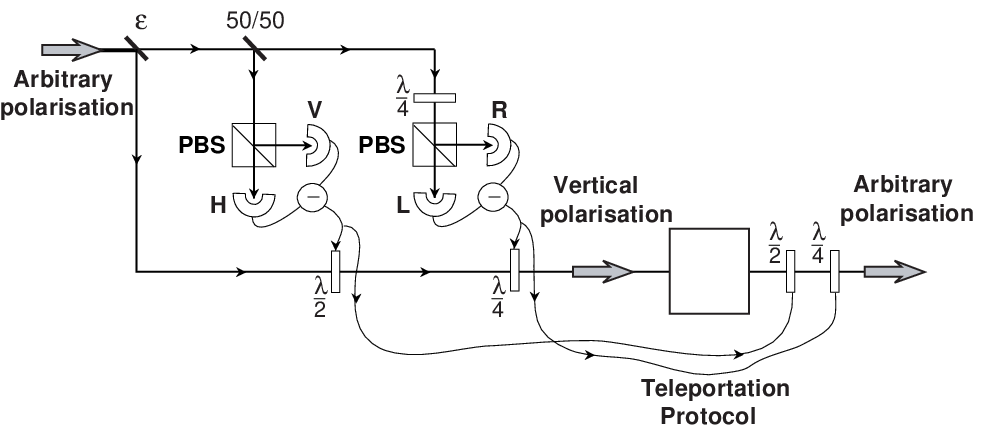
So far, we have chosen to ignore the classical amplitude of our input state. Although the fluctuations in the input polarisation are teleported by the twin teleporters, the polarisation of the input carrier field is not teleported. This is, at first thought, analogous to quadrature teleportation where the carrier amplitude, or the optical intensity, of the input beam is assumed to be unimportant in the reconstruction of the quantum state at the sideband frequency. Besides, it is relatively trivial to replicate the input intensity at the output. Interestingly however, equations (7-9) suggest that the polarisation of the input carrier field cannot be ignored in the teleportation of polarisation states. This is due to the fact that uncertainty relations of Stokes operators are directly scaled by the carrier polarisation. The carrier field polarisation consists of two amplitudes (the horizontal and vertical components) as well as one relative phase angle. Polarisation fluctuations will only be teleported properly provided the input polarisation is known and the output polarisation is set to be identical. A complete polarisation teleporter would therefore include the twin teleporters plus an optical setup presented in FIG. 4 to shift an arbitrary carrier field polarisation to a set polarisation and then, after the teleportation protocol, return it to its original polarisation.

Figure 4: Classical control system for measuring and controlling the polarisation of carrier field. This figure demonstrates that input polarisation state can be measured and fed forward to control the polarisation state of another beam. $\varepsilon$: beamsplitter with low transmittivity, H/V: horizontal/ vertical polarisation detection, R/L: right/ left circular polarisation detection, PBS: polarising beamsplitter, $\frac{\lambda}{2}$: half-wave plate, $\frac{\lambda}{4}$: quarter-wave plate. The vertical output is subsequently teleported by a chosen protocol and returned back to its original polarisation at the receiving station.

V SQD-teleporter scheme

Inspection of the Stokes operators shows that since $\hat{S_{0}}$ commutes with $\hat{S_{1}}$, $\hat{S_{2}}$ and $\hat{S_{3}}$, it can be measured with no penalty on the remaining three operators. For quadrature teleportation two squeezed beams enable teleportation of two variables, $\delta\hat{X}^{-}$ and $\delta\hat{X}^{+}$. This raises the question of whether polarisation teleportation could be achieved using only three squeezed beams (for $\hat{S_{1}}$, $\hat{S_{2}}$ and $\hat{S_{3}}$) rather than the four utilised in the previous scheme . Choosing the polarisation of the carrier beam to be vertical, causes the $\alpha_{H}$ terms in equations (4-6) to vanish, giving

$$\delta\hat{S}_{1}^{\rm SQD} = -\alpha_{V}\delta X^{+}_{V},$$ (14)

$$\delta\hat{S}_{2}^{\rm SQD} = \alpha_{V}(\delta X^{+}_{H}\cos\theta-\delta X^{-}_{H}\sin\theta),$$ (15)

$$\delta\hat{S}_{3}^{\rm SQD} = \alpha_{V}(\delta X^{-}_{H}\cos\theta+\delta X^{+}_{H}\sin\theta).$$ (16)

The linearised variances for the vertical carrier Stokes fluctuations from equations (7-9) now simplify to

$$V_{\delta\hat{S}_{1}}^{\rm SQD} = \alpha_{V}^{2}V_{V}^{+},$$ (17)

$$V_{\delta\hat{S}_{2}}^{\rm SQD} = \alpha_{V}^{2}(\cos\theta)^{2}\ V_{H}^{+}+\alpha_{V}^{2}(\sin\theta)^{2}\ V_{H}^{-}-$$ (18)

$$2\alpha_{V}^{2}\sin\theta\cos\theta\langle\delta X^{+}_{H,c}\delta X^{-}_{H,c}\rangle,$$

$$V_{\delta\hat{S}_{3}}^{\rm SQD} = \alpha_{V}^{2}(\cos\theta)^{2}\ V_{H}^{-}+\alpha_{V}^{2}(\sin\theta)^{2}\ V_{H}^{+}+$$ (19)

$$2\alpha_{V}^{2}\sin\theta\cos\theta\langle\delta X^{+}_{H,c}\delta X^{-}_{H,c}\rangle.$$

where the variances $V_{H/V}^{\pm}=V_{\rm c}^{\pm}+V_{\rm q}^{\pm}$, are the sum of classical signal and quantum fluctuation variances. The classical cross correlation terms in equations (7-9) have now reduced so that only correlations between the phase and amplitude quadratures of the horizontal input mode remain.

The phase angle $\theta$ has no affect on the classical polarisation since $\alpha_{H}=0$, therefore making the angle between $\alpha_{V}$ and $\alpha_{H}$ meaningless. It does nevertheless appear in the expressions for the variances of the Stokes operators, although the angle is not referenced to a coherent field. The situation is analogous to the case of a squeezed vacuum state where its quadrature angle, although lacking reference to a coherent amplitude, affects the variance.

The uncertainty relations in Eq. (2) are strongly affected by choosing $\langle\hat{a}_{H}\rangle=0$ since this also implies $\langle\hat{S}_{2}\rangle=\langle\hat{S}_{3}\rangle=0$. ¿From Eq. (2), the only uncertainty remaining is that between $\hat{S}_{2}$ and $\hat{S}_{3}$. Quantum teleportation of these two quantities can be achieved via a single entangled pair. $\hat{S}_{1}$ on the other hand commutes with $\hat{S}_{2}$ and $\hat{S}_{3}$ and can be determined without disturbing them, therefore its reconstruction does not require a second entangled pair. In other words, equations (15) and (16) are seen to completely decouple from equation (14). The vertical amplitude fluctuations of $\delta\hat{S}_{1}^{\rm SQD}$ can therefore be reproduced by a single quadrature (SQD) measurement [18].

The schematic of this SQD protocol is shown in FIG. 5.

Figure 5: SQD-teleporter experimental setup consisting of a direct detection SQD measurement and a quadrature teleporter circuit. Det: standard amplitude detector, + : amplitude modulator, $g_{+}$: amplitude modulator gain, PBS: polarising beamsplitter.

Vertically polarised light is incident at the input polarising beamsplitter. The bright vertical light mode is reflected and detected. The resulting photocurrent is used to control the amplitude modulation of a vertically polarised squeezed beam, SQ3. The amplitude quadrature of the modulated beam SQ3 will, in the limit of ideal squeezing and appropriate feed-forward gain, be identical to $\delta\hat{X}_{V}^{+}$, the amplitude quadrature of the the vertically polarised light at the input to the teleporter. Since $\delta\hat{S}_{1}^{\rm SQD}\propto\delta\hat{X}_{V}^{+}$ this single quadrature feed-forward loop is enough to teleport $\delta\hat{S}_{1}$ The quadrature teleportation protocol, using an EPR pair, transfers the fluctuations of $\delta\hat{S}_{2}^{\rm SQD}$ and $\delta\hat{S}_{3}^{\rm SQD}$ onto the horizontally polarised output beam EPR1 [16]. The vertical and horizontal output modes are then combined via a second polarising beamsplitter and the polarisation information is recreated. It is important to ensure that the horizontal output mode (EPR1) has much less power than the vertical output beam SQ3, in order to preserve the input polarisation.

The above scheme is not necessarily limited only to vertically polarised input states. An arbitrary input state can be rotated using a variable half and quarter-wave plate arrangement and feedback loops, such as that in FIG. 4, to ensure all of the light power is in the SQD part of the system and its polarisation is vertical. Once the protocol is complete, it can be rotated back to its original polarisation.

The amplitude squeezing of SQ3 enables, in theory, a perfect reproduction of the single amplitude quadrature fluctuation $\delta\hat{X}_{V}^{+}$. The complete polarisation teleportation system now uses only an entangled pair and one additional squeezed beam.

An interesting characteristic of the measurement of the vertical polarization is that the signal transfer is best in the limit of infinite gain. On the other hand, the conditional variance of the vertical polarisation cannot be improved as there are no correlations between the detected beam and the squeezed reconstruction beam.

It is possible however, to represent the entire system on a single T-V diagram with $T_{q}=T^{+}_{H}+T^{-}_{H}+T^{+}_{V}$ and $V_{\rm cv}=\frac{1}{3}(V^{+}_{\rm cv,H}+V^{-}_{\rm cv,H}+V^{+}_{\rm cv,V})$. Since the phase quadrature $\delta\hat{X}^{-}_{V}$ is irrelevant to the polarisation description of the state (equations (17-19)), it is reasonable not to include it in the T-V analysis, which relates to the polarisation information transferred during the teleportation process.

For simplicity, the choice of $V_{SQ3}=V_{SQ}$ is made for the remainder of this section. FIG. 6 shows a resulting three quadrature ($X_{H}^{+},\ X_{H}^{-},X_{V}^{+}$) T-V plot. For ideal squeezing of all three beams the minimum conditional variance $V_{\rm cv}\rightarrow 0$, and the maximum signal transfer coefficient $T_{q}\rightarrow 3$, can still be reached.

Figure 6: The SQD-teleporter T-V plot using only three quadratures of interest, with $V_{SQ3}=V_{SQ}$. (a) with coherent states (b) with 3 dB squeezing ($V_{\rm SQ}=0.5$), (c) with 10 dB squeezing ($V_{\rm SQ}=0.1$) and (d) Locus of unity gain points from no squeezing to perfect squeezing

In the SQD scheme, beam SQ3 needs to be amplitude squeezed in order to reduce any noise in the signal quadrature. As a result, the phase quadrature becomes very noisy as ${1}/{V_{SQ3}}\rightarrow\infty$. The unfavourable consequence of this is that the fidelity of the scheme is found to be vanishingly small. The fidelity equation (10) reduces to

$$\mathcal{F}_{\rm SQD}=\frac{2}{(1+V_{\rm SQ})\sqrt{(V_{\rm SQ3}+2)\ (\frac{1}{V_{\rm SQ3}}+1)}}$$ (20)

In fact, the maximum fidelity of the replicated quantum state is $\mathcal{F}$ = $\sqrt{(2/3)}$, attained when there is no SQ3 squeezing at all. FIG. 7 shows two possible fidelity curves, with and without SQ3 beam squeezing. The SQD-teleporter curve exceeds the results of the twin teleporters for all squeezing levels up to 80$\%$, even though less resources are used. This is because there are fewer measurement penalties in the 3 beam case. When performing classical teleportation (i.e. teleportation with coherent states in place of entanglement) of all 4 quadratures, each quadrature reconstruction will degrade the fidelity. Classical teleportation of only 3 quadratures means the fourth quadrature is not degraded and therefore does not contribute to reducing the fidelity. The classical limit in the case of the SQD protocol may then be redefined by substituting $V_{\rm SQ}=V_{\rm SQ3}=1$ in Eq. 20, giving $\mathcal{F}=1/\sqrt{6}$.

Figure 7: The fidelity curves for (a) the twin teleporter system; (b) the SQD-teleporter system with $V_{\rm SQ3}=V_{\rm SQ}$, (c) the SQD-teleporter system with no squeezing on the SQ3 beam

VI Biased entanglement teleporter scheme

Figure 8: Biased entanglement teleporter experimental setup. $\varepsilon_{1}$: the variable transmittivity beamsplitter for biased entanglement of the inputs, $\varepsilon_{2}$: the variable transmittivity beamsplitter for detection, $D_{\pm}$: amplitude/ phase homodyne detection, +/- : amplitude/ phase modulators, $g_{\pm}$: amplitude/ phase feedforward gains, PBS: polarising beamsplitter.

It is somewhat disappointing that our SQD-teleporter scheme described in section V, performs worse in terms of fidelity when the SQ3 beam is squeezed (FIG. 7(b) and (c)). In this section we present an alternative polarisation teleportation scheme that also uses three squeezed beams but can perform better than the SQD-teleporter scheme in terms of fidelity.

Here, we use the third squeezed beam to generate entanglement of the vertical polarisation. A single squeezed beam and a vacuum mode are combined on a beamsplitter (labelled $\varepsilon_{1}$), the outputs of this beamsplitter then exhibit biased entanglement [15]. That is, strong correlations are evident between the squeezed quadratures of the two outputs, but only shot noise limited correlations exist between the beams for the orthogonal quadratures [15]. One of the biased entangled beams is then mixed with the vertical mode of the input state at the second beamsplitter (labelled $\varepsilon_{2}$). The ability to choose the transmittivity of this beamsplitter allows measurements of the amplitude quadrature of the vertical signal, which is equivalent to $\delta S_{1}$, or the phase quadrature of the vertical input, which is not represented on the Poincaré sphere, or to alternatively measure any combination of the two. The signal is then detected and fed-forward to the modulators. We term this configuration biased entanglement teleportation (BET) (see FIG. 8).

The BET scheme can be thought of a modification of the twin teleporters which tries to limit the resources from four bright, squeezed beams, to only three. One EPR pair is still maximally entangled and teleports the horizontal fluctuations as before, however the vertical information on the signal is teleported with one of the squeezed beams turned off. Further, the SQD-teleporter scheme from Section V is a special case of the BET scheme and can be recovered by setting $\varepsilon_{1}=$ 1 and $\varepsilon_{2}=$ 0.

The fidelity of a BET setup surpasses the $\mathcal{F}\ =\sqrt{(2/3)}$ direct detection limit. To do this, various parameters of the system can be optimised according to the value of squeezing injected, $V^{\pm}_{\rm SQ3}$. The beamsplitter transmittivities, $\varepsilon_{1}$ and $\varepsilon_{2}$, can be changed to optimise equation (10). The amplitude modulator gain, $g_{+}$ which relates to the vertically polarised signal quadrature needs to be kept at unity. The phase modulator gain, $g_{-}$ however, relates to the quadrature with no information, and hence is optimised to minimise the reconstruction noise. Both gains are functions of $\varepsilon_{1},\varepsilon_{2}$ and the squeezing, $V_{\rm SQ3}^{\pm}$. The polarity of $g_{+}$ and the quadrature being squeezed (either $V^{-}_{\rm SQ3}$ or $V^{+}_{\rm SQ3}$), suggest four possible operating regimes. Our detailed analysis shows that three of these regimes have maximum fidelity surpassing that of the SQD-teleporter scheme. For the remainder of this section we will only discuss the best regime, which was obtained with feedforward gain of $g_{+}>$ 0, and with the input phase squeezed ($V_{\rm SQ3}^{-}<$ 1).

The improvement in the fidelity of the system occurs because at the extremes of squeezing $\varepsilon_{1}$ and $\varepsilon_{2}\rightarrow$ 0, so that almost all of the signal in the BET scheme is directed to the amplitude detector, $(D_{+}$), while most of the phase quadrature squeezing goes directly to the phase detector, $(D_{-})$. The modulation is then imprinted onto a nearly quantum noise limited beam. Some correlations exist between the detected phase fluctuations and the fluctuations of the output beam, which enable a cancellation of the output phase quadrature variance down to half the original shot noise level. The signal (amplitude) quadrature only pays the measurement penalty by coupling to a single unit of vacuum noise. For identical squeezing levels on all three beams, $V_{\rm sq}^{+}<1$, the expression for fidelity in terms of the beam splitter ratios is given by

$$\mathcal{F}_{\rm max}=\frac{\ \mathcal{A}}{\sqrt{\mathcal{B}\mathcal{C}}}\\$$ (21)

where $\mathcal{A}$, $\mathcal{B}$, and $\mathcal{C}$ are given by

$$\mathcal{A} = 2\sqrt{(\varepsilon_{2}-1)[\varepsilon_{2}(V_{\rm SQ3}^{+}-1)(\varepsilon_{1}-1)-\varepsilon_{1}(V_{\rm SQ3}^{+}-1)-1]},$$ (22)

$$\mathcal{B} = 2\varepsilon_{2}(V_{\rm SQ3}^{+}-1)\ (\varepsilon_{1}-1)-\varepsilon_{1}(V_{\rm SQ3}^{+}-1)-2,$$ (23)

$$\mathcal{C} = \varepsilon_{2}\left(3-2\varepsilon_{1}+V_{\rm SQ3}^{+}(2\varepsilon_{1}-1)\right)+2(V_{\rm SQ3}^{+}-1)\ \sqrt{\varepsilon_{2}(1-\varepsilon_{2})\varepsilon_{1}(1-\varepsilon_{1})}\ -\varepsilon_{1}(V_{\rm SQ3}^{+}-1)-3$$ (24)

Figure 9: The comparison of the fidelity curves for (a) SQD-teleporter, (b) the optimum BET scheme, (c) the optimised twin teleporters. The schemes are all equivalent at low squeezing parameter.

FIG. 9(b) illustrates the fidelity of the optimum BET scheme by varying transmittivities, $\varepsilon_{1}$ and $\varepsilon_{2}$, as a function of squeezing. The maximum reached at ideal squeezing is $\mathcal{F}=\frac{2\sqrt{2}}{3}\approx$ 0.943. As expected, unity fidelity is never reached, however for all input squeezing levels the BET scheme is better than the SQD-teleporter scheme. Furthermore, the BET scheme can surpass the performance of the twin teleporters scheme introduced in Section IV at squeezing values within experimental reach. This scheme preserves the quantum nature of the complete state well but, as will be shown shortly, when information transfer is considered it is inferior to that of SQD-teleporter scheme.

The evaluation of the transfer coefficient and conditional variance is also dependent on the optimisation of gain, beamsplitter ratios and available squeezing parameters. However the parameters optimised for fidelity, do not necessarily correspond to the best T-V result. This occurs because fidelity weights every quadrature or Stokes operator equally, whereas T-V analysis concentrates on the information containing variables $S_{1}$, $S_{2}$ and $S_{3}$. The BET system then needs to be re-optimised and again, various regimes are reached depending on the transmittivities of $\varepsilon_{1}$ and $\varepsilon_{2}$. Our analysis shows that $T_{V}^{+}$ and $V_{\rm cv}$ as a function of feedforward gain are optimised if the BET arrangement is set to recover the SQD-teleporter scheme of FIG. 6, by setting $\varepsilon_{1}=$ 1 and $\varepsilon_{2}=$ 0. Here the function $T^{+}_{V}=(4g_{+}^{2})/({4g_{+}^{2}+V_{\rm sq}^{+}})\rightarrow 1$ , as $g_{+}\rightarrow\infty$. With greater squeezing, the transfer coefficient approaches unity more rapidly as $g_{+}$ increases. The amplitude quadrature conditional variance is independent of gain $V_{\rm cv}^{+}=V_{\rm SQ3}^{+}$ and the minimum of zero occurs only in the limit of perfect squeezing.

It is clear from the above fidelity and T-V analysis that successful information transfer is not necessarily linked to an improvement in fidelity. When optimising the fidelity, the BET protocol is weighted in favour of better state overlap. This means improving the output phase noise of the SQ3 beam. Reducing this phase noise, however, means sacrificing signal and reducing the signal transfer coefficient. The decision of which characterisation method to use should be made dependent on the particular quantum information protocol, for which the teleportation scheme is to be used.

VII Optimized twin teleporter scheme

The fidelity curve as a function of squeezing for the twin teleporters in the FIG. 7(a) could also be optimised for the amplitude coded input signal considered in this paper. This can be achieved in a manner similar to the biased entanglement teleportation optimisation, by adjusting the beamsplitter transmittivities for each squeezing value. When all four inputs are equally squeezed, ($V_{SQ3}=V_{SQ}=V_{\nu}$), and the pairs are 90 degrees out of phase for best results, the fidelity is given by

$$\mathcal{F}_{\rm 4SQ}=\frac{\mathcal{D}}{\sqrt{\rm\mathcal{M}\ \mathcal{N}}}\\$$ (25)

where $\mathcal{D}$, $\mathcal{M}$, and $\mathcal{N}$ are given by

$$\mathcal{D} = 2\sqrt{V_{\rm SQ3}^{+}(\varepsilon_{2}-1)[\varepsilon_{2}\ (V_{\rm SQ3}^{+}-1)(V_{\rm SQ3}^{+}(\varepsilon_{1}-1)+\varepsilon_{1})\ +(V_{\rm SQ3}^{+})^{2}(1-\varepsilon_{1})+\varepsilon_{1}]},$$ (26)

$$\mathcal{M} = (1+V_{\rm SQ3}^{+})\left(\varepsilon_{2}(V_{\rm SQ3}^{+}-1)(1-2\varepsilon_{1})+\varepsilon_{1}(V_{\rm SQ3}^{+}-1)-V_{\rm SQ3}^{+}\right),$$

$$\mathcal{N} = \varepsilon_{2}\left(1-2V_{\rm SQ3}^{+}-2\varepsilon_{1}-(V_{\rm SQ3}^{+})^{2}(1-2\varepsilon_{1})\right)$$ (27)

$$+(1-(V_{\rm SQ3}^{+})^{2})\left(\varepsilon_{1}-2\sqrt{\varepsilon_{2}(1-\varepsilon_{2})\varepsilon_{1}(1-\varepsilon_{1})}\right)+2V_{\rm SQ3}^{+}+(V_{\rm SQ3}^{+})^{2}$$

Again, several regimes emerge, however only the optimum regime for fidelity is considered here. This is shown on FIG. 9(c). The two optimised systems of BET (FIG. 9(b)) and twin teleporters, show comparable results at lower values of the squeezing parameter, even though the twin teleporter requires more resources.

VIII Conclusion

We have investigated schemes for the teleportation of polarisation states carried by bright optical beams. We have shown that simply performing quadrature teleportation on the horizontal and vertical constituent modes separately is not optimal in terms of squeezing resources with respect to both the T-V and fidelity figures of merit. We introduce schemes that optimise the squeezing resources required for polarisation teleportation with respect to each figure of merit. We find that the optimisation is different depending on the figure of merit being used.

The difference in optimisation of the two figures of merit can be understood in the following way. When small signals are applied to the polarisation sidebands of a light field, they can be considered to be a two-mode coherent state $|\alpha_{H}\rangle|\alpha_{V}\rangle$. Due to our choice of basis, both figures of merit quantify the transfer of quantum information on the horizontal mode, however they differ in how they treat the vertical mode. The T-V analysis considers the vertical mode to be a quantum limited classical channel. On the other hand the fidelity analysis considers the vertical mode to carry quantum information on a restricted domain (i.e. $\alpha_{V}$ is restricted to be real). The appropriate figure of merit, and thus the most efficient teleportation protocol to use in a particular circumstance, depends on the way in which the quantum information is being encoded.