Structure of the Wake of a Magnetic Obstacle

Abstract

We use a combination of numerical simulations and experiments to elucidate the structure of the flow of an electrically conducting fluid past a localized magnetic field, called magnetic obstacle. We demonstrate that the stationary flow pattern is considerably more complex than in the wake behind an ordinary body. The steady flow is shown to undergo two bifurcations (rather than one) and to involve up to six (rather than just two) vortices. We find that the first bifurcation leads to the formation of a pair of vortices within the region of magnetic field that we call inner magnetic vortices, whereas a second bifurcation gives rise to a pair of attached vortices that are linked to the inner vortices by connecting vortices.

When a liquid metal moves relative to a localized magnetic field - a magnetic obstacle - the induced eddy currents produce a Lorentz force that creates vorticity. Whereas the flow pattern around a mechanical obstacle, such as the cylinder shown in Fig. 1, are well documented [2], the structure of the wake of a magnetic obstacle is poorly understood even in the seemingly simple steady state. In the present Letter we demonstrate that the first bifurcation in the flow past a magnetic obstacle leads to the formation of a vortex-pair inside the magnetic field and that the formation of attached vortices, the analog to Fig. 1$b$, is the result of a second bifurcation giving rise to a remarkably complex six-vortex pattern.

Figure 1: Streamlines of the steady flow around a solid cylinder and corresponding streamwise velocity along the centerline: (a) without vortices and (b) with attached vortices. Notice, the region of attached vortices corresponds to negative streamwise velocity.

Figure 2: (color) Magnetic obstacle (insertion) and streamwise velocity along the centerline from 3D numerical simulation ($a-c$) and experiment ($d$): N=4, Re=100 ($a$), N=11.25, Re=100 ($b$), N=11.25, Re=400 ($c$), N=11.25, Re=2000 ($d$). Dashed vertical lines mark borders of the magnetic obstacle.

Figure 3: (color). Flow streamlines in the middle plane corresponding to profiles of Fig. 2 involving inner (red $b-d$), connecting (green $c,d$), and attached (magenta $c,d$) vortices. Dashed lines mark borders of the magnetic obstacle.

Understanding the wake of a magnetic obstacle, whose prototype is shown in Fig.2, is of considerable fundamental and practical interest. On the fundamental side [3, 4, 5, 6], a magnetic obstacle represents a system with a rich variety of dynamical states whose behavior is governed by two parameters, the Reynolds number $Re=u_{0}H/\nu$ (where $u_{0}$ is velocity, $H$ is the characteristic linear size, and $\nu$ is the kinematic viscosity of the fluid) and the magnetic interaction parameter $N=\sigma HB_{0}^{2}/\rho u_{0}$ (where $\sigma$ is the electric conductivity of the fluid, $\rho$ its density and $B_{0}$ the magnitude of the magnetic field) [3]. On the practical side, spatially localized magnetic fields enjoy a variety of industrial applications [7] exemplified by electromagnetic stirring, electromagnetic brake, and non-contact flow measurement [8].

An analogy between the hydrodynamic obstacle and a braking localized magnetic field has been supposed from the beginning of Magnetohydrodynamics. However, up to now the corresponding reverse flow behind a magnetic obstacle has never been observed experimentally. The earliest 2D calculations [9] showed a kind of recirculation, but the especially designed experiments [10] failed to confirm it. Recent 2D numerical papers of Cuevas et al. revived the term ’magnetic obstacle’ and found a Karman vortex street [11] for large $Re$, as well as a vortex dipole in a creeping flow [12].

We shall derive logically, for the first time, new possible stationary magnetohydrodynamic flow patterns and illustrate them by both physical experiments and 3D numerical simulations. Technical details to reproduce our quantitative results are given to the end of the paper.

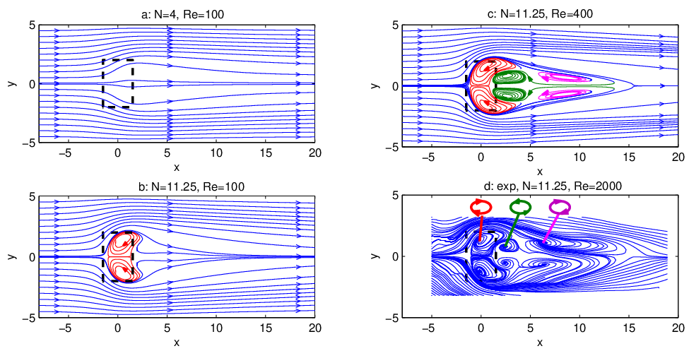
Let us recall that interaction parameter $N$ represents the ratio of the Lorentz forces to the inertial forces and Reynolds number $Re$ is the ratio of inertial and viscous forces. From this we derive that (i) the higher $N$ the stronger is the braking Lorentz force inside the obstacle and (ii) the larger $Re$ the more pronounced is the stagnant region behind the obstacle. Now we analyze all possible dependencies of streamwise velocity along the centerline (centerline curves), Fig. 2, analogously as it is shown in Fig. 1. Figure 3 illustrates these centerline curves by flow patterns obtained from 3D numerical simulation and physical experiment. It is obvious to conclude that streamwise velocity inside the magnetic obstacle is positive for small $N$ (curve $a$) and might be negative when $N$ is higher than a critical value $N_{c}^{m}$ (curves $b-d$). Past the obstacle the flow structure is analogous to that of a solid cylinder shown in Fig. 1: at low $Re$ the velocity is positive (curves $a,b$), and it might be negative when $Re$ is larger $Re_{c}(N)$ (curves $c,d$).

It is a signal for a reverse flow when a centerline curve becomes negative. Therefore, we deduce that in the most developed case there must be a pair of vortices inside the obstacle, which we call inner magnetic vortices and show by red color in Fig. 3($b-d$), and a pair of hydrodynamical attached vortices past the obstacle marked by magenta color in Fig. 3($c,d$).

Figure 4: (color) Topology of the flow involving inner (red), connecting (green), and attached (magenta) vortices, bold dashed lines mark borders of magnetic obstacle. Cross-marked are fixpoints, black lines are heteroclinic orbits.

The inner vortices and the attached vortices show the same direction of rotation determined by the main flow movement. This means that a continuous flow only can exist, if the pairs of inner and attached vortices are connected by contra-rotating connecting vortices shown by green color in Fig. 3($c,d$). These connecting vortices correspond to a local maximum of centerline curves in Fig. 2 at $x\approx 2.5$. The resulting flow structure of Fig. 3($c,d$) becomes clear from Fig. 4, where the 2D flow structure in the middle plane is organized around six hyperbolic fixpoints and their corresponding heteroclinic invariant manifolds. As can be derived from nonlinear topological dynamics [13] no other two-dimensional volume conserving and continuous differentiable flow structure is possible, in which two pairs of vortices with the same sense of rotation can coexist. The inner and connecting vortices with the surrounding invariant manifolds replace the rigid body of Fig. 1. Notice, that a virtual (magnetic) obstacle induces real vortices inside. This is a direct representation of the hydrodynamic potential theory where a real physical body is modelled by means of a virtual vortex dipole flow.

Recirculation inside the obstacle is dependent on the interaction parameter $N$ being inverse proportional to velocity. Therefore, starting from a stable flow without vortices, inner vortices and then the six-vortex pattern involving attached vortices appear by decreasing the flow rate. This is a paradoxical behavior being in contrast to the ordinary hydrodynamics where attached vortices always appear at increasing flow rate.

To confirm the foresaid theoretical finding experiments have been performed. The measured centerline velocity, curve $d$ in Fig. 2, agrees very well with simulated results in the region of the magnets. Behind the magnets there is a discrepancy which is obviously explained by the fact that the experimental $Re=2000$ is essentially larger than in 3D simulation. However, the experimental flow structure shown in Fig. 3($d$) is qualitatively the same as in Fig. 3($c$). Therefore, the found six-vortex pattern is stable in the experiments even at $Re=2000$. Both experiment and numerical simulation show that with increasing $Re$ and constant $N$ the attached vortices grow while the connecting vortices slightly shrink.

Direct quantitative comparison between experiment and simulation is not possible due to the following reasons. First, inlet flow is laminar in simulations and turbulent in experiments. Second, high experimental Hartmann number is difficult to handle in a proper 3D simulation since Hartmann layers must be finely resolved on the bottom and top walls. For qualitative comparison these factors are not important, since $Re$ number plays no role for the core flow [14] and turbulent pulsations are suppressed by magnetic field [15]. The slight spanwise asymmetry of the experimental flow, Fig. 3$d$, is due to a bend of the flow circuit in front of the channel inlet.

Let us now shortly describe some technical issues. The governing equations which were solved in the present 3D simulation to obtain Fig. 2, 3 are composed of Navier-Stokes plus Maxwell equations for moving medium and Ohm’s law. Induced magnetic field is assumed to be infinitely small compared to an external magnetic field [4]. Then, these equations are the following:

$$\frac{{\partial\textbf{u}}}{{\partial t}}+(\textbf{u}\cdot\nabla)\textbf{u}=-\nabla p+\frac{1}{Re}\triangle\textbf{u}+N(\textbf{j}\times\textbf{B}),$$

$$\textbf{j}=-\nabla\phi+\textbf{u}\times\textbf{B},\,\,\,\nabla\cdot\textbf{u}=0,\,\,\,\triangle\phi=\nabla\cdot(\textbf{u}\times\textbf{B}),$$

where $\bf{u}$ is velocity, $\bf{B}$ is external magnetic field, $\bf{j}$ is electric current density, $p$ is pressure, $\phi$ is electric potential. The above equations were solved by an own self-made 3D solver for the same rectangular duct as in the experiments. Technical numerical details are given in [14].

The experimental data presented in Fig. 2, 3 were measured by one of the authors, O.A., with the Ultrasonic Doppler Velocimeter DOP2000, on the experimental setup described in details in [15]. This setup is represented by the Ga-In-Sn eutectic alloy flowing in the rectangular duct with sizes (Length $\times$ Width $\times$ Height)=$2(L_{x}\times L_{y}\times H)$=(50 $\times$ 10 $\times$ 2). The magnets were assembled in a yoke and with horizontal sizes (Length $\times$ Width)=$2(M_{x}\times M_{y})$=(3 $\times$ 4) and distance between the poles $h=3$. All numbers are in centimeters. Magnetic field strength measured in the center of the magnetic gap is $B_{0}=0.4$T.

$Re$ and $N$ through the paper are defined with the parameters $H$, $u_{0}$ and $B_{0}$ equal to half-height of the duct, the mean flow velocity, and field intensity measured in the center of the magnetic gap, correspondingly.

External magnetic field was modelled as a field from two permanent magnets occupying a space $\Omega=\{|x|\leq M_{x},|y|\leq M_{y},|z|>=h\}$, then ${\bf B(r)}=\nabla\int_{\Omega}{\bf B_{d}(r,r^{\prime})}d{\bf r^{\prime}}$, where ${\bf B_{d}(r,r^{\prime})}=\partial_{z^{\prime}}(1/|{\bf r}-{\bf r^{\prime}}|)$ is a field created by a single magnetic dipole. After algebraic calculations:

$$B_{\gamma}(x,y,z)=\sum_{i,j,k=\pm 1}ijk\,F_{\gamma}(x-iM_{x},y-jM_{y},z-kh),$$

where $\gamma=x,y,z$ are for the magnetic field components, $F_{x}(x,y,z)=\tanh^{-1}\frac{y}{r}$, $F_{y}(x,y,z)=\tanh^{-1}\frac{x}{r}$, $F_{z}(x,y,z)=\tan^{-1}\frac{zr}{xy}$, and $r=(x^{2}+y^{2}+z^{2})^{-1/2}$. Such an analytic approach is rather precise, as was tested by comparing the calculated magnetic field with the field measured experimentally.

Figure 5: (color). (a): Stability of inner magnetic vortices in dependence on constrainment $\kappa$ and interaction parameter $N$ at fixed $Re=100$. (b): Global stability diagram giving the existence regions of all three flow types described in this Letter in dependence on ($Re$, $N$) at fixed $\kappa=0.4$.

Let us now turn to final results presented as stability diagrams in Fig. 5. They summarize the flow behavior around the magnetic obstacle dependent on the three parameters $Re$, $N$ and $\kappa$, where $\kappa=M_{y}/L_{y}$ is the constrainment ratio between the lateral size of the magnet, $2M_{y}$, and the width of the channel, $2L_{y}$. The foresaid simulated and experimental results correspond to a constrainment ratio of $\kappa=0.4$.

In Fig.5 the constrainment factor is varied for the Reynolds number $Re=100$. The less is $\kappa$, the less is the influence of side walls. The case of $\kappa\rightarrow 0$ corresponds to a free flow. The larger is $\kappa$, the more spanwise uniform is the braking Lorentz force. Therefore, in order to induce inner vortices at larger $\kappa$ it is necessary to apply a larger critical interaction parameter $N_{c}^{m}$ as one can see in Fig. 5. At $\kappa\leq 0.5$ the critical value of $N_{c}^{m}$ is of the same order of magnitude, $N_{c}^{m}\approx 6$, and after $\kappa\approx 0.8$ rapidly increases up to $N_{c}^{m}\approx 110$ at $\kappa=1$. We believe that it is impossible to provoke magnetic vortices at high $\kappa$ corresponding to spanwise uniform magnetic field.

At small constrainment ratio ($\kappa\ll 1$) and fixed $M_{x}$ the magnetic obstacle becomes very slim (magnetic blade) compared to the channel width. Then, attached vortices are not formed because of well streamlined shape of the blade, while the magnetic vortices are originated as before. Now, these magnetic vortices are elongated along side walls of the magnetic blade and are expanded in spanwise direction if interaction parameter $N$ increases.

Finally we present in Fig. 5 the stability diagram for $\kappa=0.4$. It shows, derived from a series of 3D simulation and experiments, bifurcation lines $N_{c}^{m}(Re)$ and $N_{c}^{h}(Re)$ separating the existence regions of flow without vortices (I), with inner vortices (II), and flow including inner magnetic vortices, connecting vortices and attached vortices (III). To depict the borders between regions I-III we have calculated several foothold points given in Fig. 5 by filled symbols. The open triangle symbol at $Re=4700$ was obtained experimentally. Bifurcation points were derived by monitoring the first (for inner) respective second (for attached vortices) minimum on centerline curves as shown in Fig. 2. These minima must be exactly equal to zero at the bifurcation between two flow patterns. The first bifurcation takes place slightly above $N\approx 5$ and is almost independent of $Re$. If the magnetic vortices are present, a minimum Reynolds number, $Re_{c}^{m}$, is necessary for the second bifurcation to the appearance of attached vortices analogously to ordinary hydrodynamics. Since we have never observed attached vortices in the simulation with $Re=100$ and $N\leq 36$, $Re_{c}^{m}$ is given near 100. A series of experiments at various $Re$ resulted in a critical value of $Re_{c}\approx 4700$ for inner vortices which corresponds to $N_{c}^{m}\approx 5$ fitting well to the numerical values.

In summary, new phenomena are discovered for conducting liquid flowing through a magnetic obstacle. One is the appearance of stable inner vortices inside the obstacle at magnetic interaction parameter $N\geq N_{c}^{m}$. The other is a new six-vortex flow pattern appearing at $N\geq N_{c}^{h}(Re)$. This pattern is composed of three pairs of vortices: inner, connecting, and attached. All the vortices are found both in 3D numerical simulation and in physical experiments.

References

- [1] E-mail: evgeny.votyakov@tu-ilmenau.de
- [2] R. Feynman, R. Leighton, and M. Sands, Lectures on physics. Vol II (Addison-Wesley, 1964).
- [3] J. A. Shercliff, The theory of electromagnetic flow-measurement (Cambridge University Press, 1962).
- [4] P. H. Roberts, An introduction to Magnetohydrodynamics (Longmans, Green, New York, 1967).
- [5] P. A. Davidson, An introduction to Magnetohydrodynamics (Cambridge University Press, 2001).
- [6] R. Moreau, Magnetohydrodynamics (Kluwer, 1990).
- [7] P. Davidson, Annual Review of Fluid Mechanics 31, 273 (1999).
- [8] A. Thess, E. V. Votyakov, and Y. Kolesnikov, Phys. Rev. Lett. 96, 164501 (2006).
- [9] Y. M. Gelfgat, D. E. Peterson, and E. V. Shcherbinin, Magnetohydrodynamics 14, 55 (1978).
- [10] Y. M. Gelfgat and S. V. Olshanskii, Magnetohydrodynamics 14, 151 (1978).
- [11] S. Cuevas, S. Smolentsev, and M. Abdou, J. Fluid Mech 553, 227 (2006a).
- [12] S. Cuevas, S. Smolentsev, and M. Abdou, Phys. Rev. E (2006b).
- [13] J. Guckenheimer and P. Holmes, Nonlinear Oscillations, Dynamical Systems and Bifurcations of Vector Fields (Springer Verlag, New York, 1983).
- [14] E. V. Votyakov and E. Zienicke, Fluid Dynamics and Materials Processing 3, 1 (2007).
- [15] O. Andreev, Y. Kolesnikov, and A. Thess, Phys. Fluids 18, 065108 (2006).