Understanding transverse coherence properties of X-ray beams in third generation Synchrotron Radiation sources

Abstract

This paper describes a theory of transverse coherence properties of Undulator Radiation. Our study is of very practical relevance, because it yields specific predictions of Undulator Radiation cross-spectral density in various parts of the beamline. On the contrary, usual estimations of coherence properties assume that the undulator source is quasi-homogeneous, like thermal sources, and rely on the application of van Cittert-Zernike (VCZ) theorem, in its original or generalized form, for calculating transverse coherence length in the far-field approximation. The VCZ theorem is derived in the frame of Statistical Optics using a number of restrictive assumptions: in particular, the quasi-homogeneous assumption is demonstrated to be inaccurate in many practical situations regarding undulator sources. We propose a technique to calculate the cross-spectral density from undulator sources in the most general case. Also, we find the region of applicability of the quasi-homogeneous model and we present an analytical expression for the cross-spectral density which is valid up to the exit of the undulator. For the case of more general undulator sources, simple formulas for the transverse coherence length, interpolated from numerical calculations and suitable for beamline design applications are found. Finally, using a simple vertical slit, we show how transverse coherence properties of an X-ray beam can be manipulated to obtain a larger coherent spot-size on a sample. This invention was devised almost entirely on the basis of theoretical ideas developed throughout this paper.

DEUTSCHES ELEKTRONEN-SYNCHROTRON

in der HELMHOLTZ-GEMEINSCHAFT

DESY 05-109

June 2005

Gianluca Geloni, Evgeni Saldin, Evgeni Schneidmiller and Mikhail Yurkov

Deutsches Elektronen-Synchrotron DESY, Hamburg ISSN 0418-9833 NOTKESTRASSE 85 - 22607 HAMBURG

1 Introduction

In recent years, continuous evolution of third generation light sources has allowed dramatic increase of brilliance with respect to older designs, which has triggered a number of new techniques and experiments unthinkable before. Among the most exciting properties of today third generation facilities is the high flux of coherent X-rays provided. The availability of intense coherent X-ray beams has fostered the development of new coherence-based techniques like fluctuation correlation dynamics, phase imaging, coherent X-ray diffraction (CXD) and X-ray holography. In this context, understanding the evolution of transverse coherence properties of Synchrotron Radiation (SR) along the beam line is of fundamental importance.

In general, when dealing with this problem, one should account for the fact that Synchrotron Radiation is a random statistical process. Therefore, the evolution of transverse coherence properties should be treated in terms of probabilistic statements: the shot noise in the electron beam causes fluctuations of the beam density which are random in time and space. As a result, the radiation produced by such a beam has random amplitudes and phases.

Statistical Optics [5, 6, 10] affords convenient tools to deal with fluctuating electromagnetic fields in an appropriate way. Among the most important quantities needed to describe coherent phenomena in the framework of Statistical Optics is the correlation function of the electric field. In any interference experiment one needs to know the system (second order) correlation function of the signal at a certain time and position with the signal at another time and position. Alternatively, and equivalently, one can describe the same experiment in frequency domain. In this case one is interested in the correlation function of the Fourier transform of the time domain signal at a certain frequency and position with the Fourier transform of the time domain signal at another frequency and position. The signal one is interested to study is, indeed, the Fourier transform of the original signal in time domain. In SR experiments the analysis in frequency domain is much more natural than that in the time domain. In fact, up-to-date detectors are limited to about $100$ ps time resolution and they are by no means able to resolve a single X-ray pulse in time domain. They work, instead, by counting the number of photons at a certain frequency over an integration time longer than the radiation pulse. Therefore, in this paper we will deal with signals in the frequency domain and we will often refer to the ”Fourier transform of the electric field” simply as ”the field”.

For some particular experiment one may be interested in higher order correlation functions (for instance, in the correlation between the intensities) which, in general, must be calculated separately. In the particular case when the field fluctuations can be described as a Gaussian process, the field is often said to obey Gaussian statistics. In this case, with the help of the Moment Theorem [5] one can recover correlation functions of any order from the knowledge of the second order one: this constitutes a great simplification to the task of describing coherence properties of light. A practical example of a field obeying Gaussian statistics is constituted by the case of polarized thermal light. This is more than a simple example: in fact, Statistical Optics has largely developed in connection with problems involving optical sources emitting thermal light like the sun, other stars, or incandescent lamps. As a consequence, Gaussian statistics is often taken for granted. Anyway, it is not a priori clear wether Synchrotron Radiation fields obey it or not; our analysis will show that Synchrotron Radiation is indeed a Gaussian random process. Therefore, as is also the case for polarized thermal light and any other signal obeying Gaussian statistics, when we deal with Synchrotron Radiation the basic quantity to consider is the second order correlation function of the field. Moreover, as already discussed, in Synchrotron Radiation experiments it is natural to work in the space-frequency domain, so that we will focus, in particular, on the second order correlation function in the space-frequency domain.

Besides obeying Gaussian statistics, polarized thermal light has two other specific properties allowing simplifications of the theory: the first is stationarity and the second is quasi-homogeneity. Exactly as the property of Gaussian statistics, also stationarity and quasi-homogeneity of the source are usually taken for granted in Statistical Optics problems but, unlike it, they do not belong, in general, to Synchrotron Radiation fields. In fact, as we will show, Synchrotron radiation fields are intrinsically non-stationary and not always quasi-homogeneous. Nevertheless, up to now it has been a widespread practice to assume that undulator sources are completely incoherent (i.e. homogeneous) and to apply the well known van Cittert-Zernike (VCZ) theorem for calculating the degree of transverse coherence in the far-field approximation [1]. Using the VCZ theorem, the electric field cross-correlation function in the far field is usually calculated (aside for a geometrical phase factor) as a Fourier transformation of the intensity distribution of the source, customarily located at the exit of the undulator.

Although the VCZ theorem only deals with completely incoherent sources, there exists an analogous generalized version of it which allows to extend the treat the case of quasi-homogeneous sources as well. Actually there is no unambiguous choice of terminology in literature regarding the scope of the VCZ theorem. For instance, a very well-known textbook [6] reports of a ”Zernike-propagation” equation dealing with any distance from the source. Also, sometimes [5], the generalized VCZ theorem is referred to as Schell’s theorem (and also used in some paper [2]). In this paper we will refer to the VCZ theorem and its generalized version only in the limit for a large distance from the source and for, respectively, homogeneous and quasi-homogeneous sources. However, irrespectively of different denominations, the fundamental fact holds, that once a cross-correlation function is known on a given source plane it can be propagated through the beamline at any distance from the source. It should be noted that, from this viewpoint, a source simply denotes an initial plane down the beamline from which the cross-correlation function is propagated further. Then, the position of the source down the beamline is suggested only on the ground of opportunity. On the contrary, when dealing with the VCZ theorem, the source must be (quasi)-homogeneous which explains the customary location at the exit of the undulator.

In some cases, the VCZ theorem or its generalized version may provide a convenient method for calculating the degree of transverse coherence in various parts of the beamline once the transverse coherence properties of the photon beam are specified at the exit of the undulator, that is at the source plane. In most SR applications though, such treatment is questionable. First, the source (even at the exit of the undulator) may not be quasi-homogeneous. Second, even for specific sets of problem parameters where the quasi-homogeneous model is accurate, the specification of the far-field zone depends not only on the electron beam sizes, but also on the electron beam divergencies (in both direction) and on the intrinsic divergence of the radiation connected with the undulator device. At the time being, widespread and a-critical use of the VCZ theorem and its generalization shows that there is no understanding of transverse coherence properties of X-ray beams in third generation Synchrotron Radiation sources.

If, on the one hand, the definition of the far-zone and the possible non quasi-homogeneity of SR sources constitute serious problems in the description of the coherence properties of Synchrotron light, on the other hand the intrinsic non-stationarity of the SR process does not play a very important role. In particular, as we will show, assumption of a minimal undulator bandwidth much larger than the characteristic inverse bunch duration (which is always verified in practice) allows to separate the correlation function in space-frequency domain in the product of two functions. The first function is a spectral correlation describing correlation in frequency. The second function describes correlation in space and is well-known also in the case of stationary processes as the cross-spectral density of the process. Then, the cross-spectral density can be studied independently at any given frequency giving information on the spatial correlation of the field. Subsequently, the knowledge of the spectral correlation function brings back the full expression for the space-frequency correlation.

In this paper we aim at the development of a theory of transverse coherence capable of providing very specific predictions, relevant to practice, regarding the cross-spectral density of undulator radiation at various positions along the beam-line. A fully general study of undulator sources is not a trivial one. Difficulties arise when one tries to include simultaneously the effect of intrinsic divergence of the radiation due to the presence of the undulator, of electron beam size and electron beam divergence into the insertion device. The full problem, including all effects, poses an unsolvable analytical challenge, and numerical calculations are to be preferred. Generally, the cross-spectral density of the undulator radiation is controlled by nine physical parameters which model both the electron beam and the undulator: the horizontal and vertical geometrical emittances of the electron beam $\epsilon_{x,y}$, the horizontal and vertical minimal betatron functions $\beta_{x,y}^{o}$, the observation distance down the beamline $z_{o}$, the observation frequency $\omega$, the undulator resonant frequency $\omega_{o}$, the undulator length $L_{w}$ and the length of the undulator period $\lambda_{w}$.

We will make a consistent use of dimensional analysis. Dimensional analysis of any problem, performed prior to analytical or numerical investigations, not only reduces the number of independent terms, but also allows one to classify the grouping of dimensional variables in a way that is most suitable for subsequent study. The algorithm for calculating the cross-spectral density can be formulated as a relation between dimensionless quantities. After appropriate normalization, the radiation cross-spectral density from an undulator device is described by six dimensionless quantities: the normalized emittances $\hat{\epsilon}_{x,y}=\omega_{o}\epsilon_{x,y}/c$, the normalized betatron functions $\hat{\beta}_{x,y}=\beta_{x,y}^{o}/L_{w}$, the normalized observation distance $\hat{z}_{o}=z_{o}/L_{w}$ and the normalized detuning parameter $\hat{C}=2\pi N_{w}(\omega-\omega_{o})/\omega_{o}$, where $N_{w}=L_{w}/\lambda_{w}$ is the number of undulator periods.

At some point in this work we will find it convenient to pose $\hat{C}=0$. In other words we will assume that parameters are tuned at perfect resonance. It is relevant to note that even under this simplifying assumptions, conditions for the undulator source to be quasi-homogeneous still include four parameters $\hat{\epsilon}_{x,y}$ and $\hat{\beta}_{x,y}$. For storage rings that are in operation or planned in the $\mathrm{\AA}$ngstrom wavelength range, the parameter variation of $\hat{\epsilon}_{x}\sim 10-10^{3}$, $\hat{\epsilon}_{y}\sim 10^{-1}-10$, $\hat{\beta}_{x,y}\sim 10^{-1}-10$ are possible: these include many practical situations in which the assumption of quasi-homogeneous sources and, therefore the (generalized) VCZ theorem, is not accurate.

In this paper we will first deal with the most general case of non-homogeneous sources. In fact, from a practical viewpoint, it is important to determine the cross-spectral density as a function of $\hat{\epsilon}_{x,y}$, $\hat{\beta}_{x,y}$, $\hat{C}$ and $\hat{z}_{o}$. Once a general expression for the cross-spectral density is found, it can be used as a basis for numerical calculations. A second goal of this work is to find the region of applicability of the quasi-homogeneous source model (i.e. of the generalized VCZ theorem) which will arise automatically from the dimensional analysis of the problem. Finally, we will derive analytical expressions for the cross-spectral density at $\hat{C}=0$ in various parts of the beamline.

Results may also be obtained using numerical techniques alone, starting from the Lienard-Wiechert expressions for the electromagnetic field and applying the definition of the field correlation function without any analytical manipulation. Yet, computer codes can calculate properties for a given set of parameters, but can hardly improve physical understanding, which is particularly important in the stage of planning experiments: understanding of correct approximations and their region of applicability with the help of a consistent use of dimensional analysis can simplify many tasks a lot, including practical and non-trivial ones. Moreover, at the time being, no code capable to deal with transverse coherence problems has been developed at all.

It should be noted that some theoretical attempt to follow this path has been proposed in [4]. Among the results of that paper is the fact that van Cittert-Zernike theorem could not be applied unless the electron beam divergence is much smaller than the diffraction angle, which is never verified in practice in the horizontal plane. We will show that this conclusion is incorrect.

We organize our work as follows. After this Introduction, in Section 2 we present a second-order theory of coherence for fields generated by Synchrotron Radiation sources. In Section 3 we give a derivation of the cross-spectral density for undulator-based sources in reduced units. Subsequently, we analyze the evolution of the cross-spectral density function through the beamline in the limit for $\hat{C}=0$. A particular case of quasi-homogeneous sources and its applicability region is treated under several simplifying assumptions in Section 4. Effects of the vertical emittance on the cross-spectral density are discussed in detail in Section 5, while a treatment of some non quasi-homogeneous source is given in the following Section 6. Obtained results include approximate design formula capable of describing in very simple terms the evolution of the coherence length along the beamline in many situation of practical interest. A good physical insight is useful to identify possible applications of given phenomena. In particular in Section 7 we selected one practical application to exploit the power of our approach. We show that, by means of a simple vertical slit, it is possible to manipulate transverse coherence properties of an X-ray beam to obtain a convenient coherent spot-size on the sample. This invention was devised almost entirely on the basis of theoretical ideas of rather complex and abstract nature which have been described in this paper. Finally, in Section 8, we come to conclusions.

2 Second-order coherence theory of fields generated by Synchrotron Radiation sources

2.1 Thermal light and Synchrotron Radiation: some concepts and definitions

A great majority of optical sources emits thermal light. Such is the case of the sun and the other stars, as well as of incandescent lamps. This kind of radiation consists of a large number of independent contributions (radiating atoms) and is characterized by random amplitudes and phases in space and time. The electromagnetic fields can be then conveniently described in terms of Statistical Optics, a branch of Physics that has been intensively developed during the last few decades. Today one can take advantage of a lot of existing experience and theoretical basis for the descriptions of fluctuating electromagnetic fields [5, 6].

Figure 1: Light intensity from an incandescent lamp driven by a constant electric current. A statistically stationary wave has an average that does not vary with time.

Consider the light emitted by a thermal source passing through a polarization analyzer (see Fig. 1). Properties of polarized thermal light are well-known in Statistical Optics, and are referred to as properties of completely chaotic, polarized light [5, 6]. Thermal light is a statistical random process and statements about such process are probabilistic statements. Statistical processes are handled using the concept of statistical ensemble, drawn from Statistical Mechanics, and statistical averages are performed indeed, over many ensembles, or realizations, or outcomes of the statistical process under study.

Polarized thermal light is a very particular kind of random process in that it is Gaussian, stationary and ergodic. Let us discuss these characteristics in more detail.

The properties of Gaussian random processes are well-known in Statistical Optics. For instance, the real and imaginary part of the complex amplitudes of the electric field from a polarized thermal source have Gaussian distribution, while the instantaneous radiation power fluctuates in accordance with the negative exponential distribution. Gaussian statistics alone, guarantees that higher-order correlation functions can be expressed in terms of second-order correlation functions. Moreover, it can be shown [5] that a linearly filtered Gaussian process is also a Gaussian random process. As a result, the presence of a spectral filter (monochromator) and a spatial filter as in the system depicted in Fig. 1 do not change the statistics of the signal, because they simply act as linear filters.

Stationarity is a subtle concept. There are different kinds of stationarity. Strict-stationarity means that all ensemble averages are independent on time. Wide-sense stationarity means that the signal average is independent on time and that the second order correlation function in time depends only on the difference of the observation times. However, for Gaussian processes strict and wide-sense stationarity coincide [5, 6]. As a consequence of the definition of stationarity, necessary condition for a certain process to be stationary is that the signal last forever. Yet, if a signal lasts much longer than its coherence time $\tau_{c}$ (which fixes the short-scale duration of the field fluctuations) and it is observed for a time much shorter than its duration $\sigma_{T}$, but much longer than its coherence time it can be reasonably considered as everlasting and it has a chance to be stationary as well, as in the case of thermal light.

Ergodicity is a stronger requirement than stationarity. Qualitatively, we may state that if, for a given random process all ensemble averages can be substituted by time averages, the process under study is said to be ergodic: all the statistical properties of the process can be derived from one single realization. A process must be strictly stationary in order to be ergodic. There exist stationary processes which are not ergodic. One may consider, for instance, the random constant process: this is trivially strictly stationary, but not ergodic because a single (constant) realization of the process does not allow one to characterize the process from a statistical viewpoint. However, this is a pathologic case when both the coherence time $\tau_{c}$ and the duration time of the signal $\sigma_{T}$ are infinite. On the contrary, a stationary process like the radiation from an incandescent lamp driven by a constant current has, virtually, infinite duration. In this case different ensembles are simply different observations, for given time intervals, of the same, statistically identical phenomenon: then, the concept of ensemble average and time average are equivalent and the process is also ergodic.

Statistical Optics was developed starting with signals characterized by Gaussian statistics, stationarity and ergodicity. Let us consider any Synchrotron radiation source. Like thermal light, also Synchrotron Radiation is a random process. In fact, relativistic electrons in a storage ring emit Synchrotron Radiation passing through bending magnets or undulators. The electron beam shot noise causes fluctuations of the beam density which are random in time and space from bunch to bunch. As a result, the radiation produced has random amplitudes and phases. As already declared in the Introduction we will demonstrate that the SR field obeys Gaussian statistics. In contrast with thermal light though, Synchrotron Radiation is intrinsically non-stationary (and, therefore, non-ergodic) because even if its short pulse duration cannot be resolved by detectors working in the time domain, it can nonetheless be resolved by detectors working in frequency domain. For this reason, in what follows the averaging brackets $\langle...\rangle$ will always indicate the ensemble average over bunches.

Figure 2: The intensity of an X-ray beam from a Synchrotron Radiation source. A statistically non-stationary wave has a time-varying intensity averaged over an ensemble of bunches.

In spite of differences with respect to the simpler case of thermal light, as we will see in this paper, also Synchrotron Radiation fields can be described in terms of Statistical Optics. Fig. 2 shows the geometry of the experiment under consideration. The problem is to describe the statistical properties of Synchrotron Radiation at the detector installed after the spatial and spectral filters. Radiation at the detector consists of a carrier modulation of frequency $\omega$ subjected to random amplitude and phase modulation. The Fourier decomposition of the radiation contains frequencies spread about the monochromator bandwidth $\Delta\omega_{\mathrm{m}}$: it is not possible, in practice, to resolve the oscillations of the radiation fields which occur at the frequency of the carrier modulation. It is therefore appropriate, for comparison with experimental results, to average the theoretical results over a cycle of oscillations of the carrier modulation.

Figure 3: Reciprocal width relations of Fourier transform pairs.

Fig. 3 gives a qualitative illustration of the type of fluctuations that occur in cycle-averaged Synchrotron Radiation beam intensity. Within some characteristic time, a given random function appears to be smooth, but when observed at larger scales the same random function exhibits ”rough” variations. The time scale of random fluctuations is the coherence time $\tau_{c}$. When $\tau_{c}\ll\sigma_{T}$ the radiation beyond the monochromator is partially coherent. This case is shown in Fig. 3: there, we can estimate $\tau_{c}\simeq\Delta\omega_{\mathrm{m}}^{-1}$. If the radiation beyond the monochromator is partially coherent, a spiky spectrum is to be expected. The nature of the spikes is easily described in terms of Fourier transform theory. We can expect that the typical width of the spectrum envelope should be of order of $\Delta\omega/\omega\sim(\tau_{c}\omega)^{-1}$. Also, the spectrum of the radiation from a bunch with typical duration $\sigma_{T}$ at the source plane should contain spikes with characteristic width $\Delta\omega/\omega\simeq(\omega\sigma_{T})^{-1}$, as a consequence of the reciprocal width relations of Fourier transform pairs (see, again, Fig. 3).

2.2 Second-order correlations in space-frequency domain

We start our discussion in the most generic way possible, considering a fixed polarization component of the Fourier transform at frequency $\omega$ of the electric field produced at location $(z_{o},\vec{r}_{\bot o})$, in some cartesian coordinate system, by a given collection of sources. We will denote it with ${\bar{E}}_{\bot}(z_{o},\vec{r}_{\bot o},\omega)$ and it will be linked to the time domain field ${{E}}_{\bot}(z_{o},\vec{r}_{\bot o},t)$ through the Fourier transform

$$\bar{{E}}_{\bot}(\omega)=\int_{-\infty}^{\infty}dt{{E}}_{\bot}(t)e^{i\omega t}~,$$ (3)

so that

$${{E}}_{\bot}(t)={1\over{2\pi}}\int_{-\infty}^{\infty}d\omega\bar{{E}}_{\bot}(\omega)e^{-i\omega t}~.$$ (4)

This very general collection of sources includes the case of an ultra relativistic electron beam going through a certain magnetic system and in particular an undulator, which is our case of interest. In this case $z_{o}$ is simply the observation distance along the optical axis of the system and $\vec{r}_{\bot o}$ are the transverse coordinates of the observer on the observation plane. The contribution of the $k$-th electron to the field Fourier transform at the observation point depends on the transverse offset $({l}_{xk},{l}_{yk})$ and deflection angles $(\eta_{xk},\eta_{yk})$ that the electron has at the entrance of the system with respect to the optical axis. Moreover, an arrival time $t_{k}$ at the system entrance has the effect of multiplying the field Fourier transform by a phase factor $\exp{(i\omega t_{k})}$ (that is, in time domain the electric field is retarded by a time $t_{k}$). At this point we do not need to specify explicitly the dependence on offset and deflection. The total field Fourier transform can be written as

$${\bar{E}}_{\bot}(z_{o},\vec{r}_{\bot o},\omega)=\sum_{k=1}^{N}\bar{E}_{s\bot}(\vec{\eta}_{k},\vec{l}_{k},z_{o},\vec{r}_{\bot o},\omega)\exp{(i\omega t_{k})}~,$$ (5)

where $\vec{\eta}_{k},\vec{l}_{k}$ and $t_{k}$ are random variables and $N$ is the number of electrons in the beam. It follows from Eq. (5) that the Fourier transform of the Synchrotron Radiation pulse at a fixed frequency and a fixed point in space is a sum of a great many independent contributions, one for each electron, of the form $\bar{E}_{s\bot}(\vec{\eta}_{k},\vec{l}_{k},z_{o},\vec{r}_{\bot o},\omega)\exp{(i\omega t_{k})}$. For simplicity we make three assumptions about the statistical properties of elementary phasors composing the sum, which are generally satisfied in Synchrotron Radiation problems of interest.

1) We assume that for a beam circulating in a storage ring random variables $t_{n}$ are independent from $\vec{\eta}_{n}$ and $\vec{l}_{n}$. This is always verified, because the random arrival times of electrons, due to shot noise, do not depend on the electrons offset and deflection with respect to the $z$-direction. Eq. (5) states that the $k$-th elementary contribution to the total ${\bar{E}}_{\bot}$ can be written as a product of the complex phasors $\exp{(i\omega t_{k})}$, and $\bar{E}_{s\bot}$ that, in its turn, can be written as a product of modulus and phase as $\bar{E}_{s\bot}(\vec{\eta}_{k},\vec{l}_{k},z_{o},\vec{r}_{\bot o},\omega)=\mid\bar{E}_{s\bot k}\mid\exp{(i\phi_{k})}$. Under the assumption of statistical independence of $t_{n}$ from $\vec{\eta}_{n}$ and $\vec{l}_{n}$ the complex phasors $\exp{(i\omega t_{k})}$, and $\bar{E}_{s\bot}$ are statistically independent of each other and of all the other elementary phasors for different values of $k$. The ensemble average of a given function $f$ of random variables $\vec{\eta}_{n}$, $\vec{l}_{n}$ and $t_{n}$ is by definition:

$$\langle f(\vec{\eta}_{n},\vec{l}_{n},t_{n})\rangle=\int_{-\infty}^{\infty}d\eta_{xn}\int_{-\infty}^{\infty}d\eta_{yn}\int_{-\infty}^{\infty}dl_{xn}\int_{-\infty}^{\infty}dl_{yn}\int_{-\infty}^{\infty}dt_{n}$$ (6)

$$\times f(\vec{\eta}_{n},\vec{l}_{n},t_{n})P(\vec{\eta}_{n},\vec{l}_{n},t_{n})~,$$ (7)

where $P(\vec{\eta}_{n},\vec{l}_{n},t_{n})$ is the probability density distribution in the joint random variables $\vec{\eta}_{n}$, $\vec{l}_{n}$, $t_{n}$. Independence of $t_{n}$ from $\vec{\eta}_{n}$ and $\vec{l}_{n}$ allows us to write

$$P(\vec{\eta}_{n},\vec{l}_{n},t_{n})=F_{\eta_{x},l_{x}}(\eta_{xn},l_{xn})F_{\eta_{y},l_{y}}(\eta_{yn},l_{yn})F_{t}(t_{n})~,$$ (8)

where we also assumed that the distribution in the horizontal and vertical planes are not correlated. Since electrons arrival times are completely uncorrelated from transverse coordinates and offsets, the shapes of $F_{\eta_{x},l_{x}}$, $F_{\eta_{y},l_{y}}$ and $F_{t}$ are the same for all electrons.

2) We assume that the random variables $\mid\bar{E}_{s\bot k}\mid$ (at fixed frequency $\omega$), are identically distributed for all values of $k$, with a finite mean $\langle\mid\bar{E}_{s\bot k}\mid\rangle$ and a finite second moment $\langle\mid\bar{E}_{s\bot k}\mid^{2}\rangle$. This is always the case in practice because electrons are identical particles.

3) We assume that the electron bunch duration $\sigma_{T}$ is large enough so that $\omega\sigma_{T}\gg 1$: under this assumption the phases $\omega t_{k}$ can be regarded as uniformly distributed on the interval $(0,2\pi)$. The assumption $\omega\sigma_{T}\gg 1$ is justified by the fact that $\omega$ is the undulator resonant frequency, which is high enough to guarantee that $\omega\sigma_{T}\gg 1$ for any practical choice of $\sigma_{T}$.

Figure 4: Amplitude and phase of the resultant vector (total complex amplitude) formed by a large number of complex phasors having random length and random phase.

The formal summation of phasors with random lengths and phases is illustrated in Fig. 4. Under the three previously discussed assumptions we can use the central limit theorem to conclude that the real and the imaginary part of $\bar{E}_{\bot}$ are distributed in accordance to a Gaussian law. Detailed proof of this fact is given in Appendix A. As a result, Synchrotron Radiation is a Gaussian random process and second-order field correlation function is all we need in order to specify the field statistical properties. In fact, as already remarked, higher-order correlation functions can be expressed in terms of second-order correlation functions.

In Synchrotron Radiation experiments with third generation light sources detectors are limited to about $100$ ps time resolution and are by no means able to resolve a single X-ray pulse in time domain: they work, instead, by counting the number of photons at a certain frequency over an integration time longer than the pulse. Therefore, for Synchrotron Radiation related issues the frequency domain is much more natural a choice than the time domain, and we will deal with signals in the frequency domain throughout this paper. The knowledge of the second-order field correlation function in frequency domain

$$\Gamma_{\omega}(z_{o},\vec{r}_{\bot o1},\vec{r}_{\bot o2},\omega,\omega^{\prime})=\left<{\bar{E}}_{\bot}(z_{o},\vec{r}_{\bot o1},\omega){\bar{E}}^{*}_{\bot}(z_{o},\vec{r}_{\bot o2},\omega^{\prime})\right>~,$$ (9)

is all we need to completely characterize the signal from a statistical viewpoint. For the sake of completeness it is nonetheless interesting to remark that it is possible (and often done, in Statistical Optics) to give equivalent descriptions of the process in time domain as well. First, note that the time domain process ${E}_{\bot}(t)$ is linked to ${\bar{{E}}}_{\bot}(\omega)$ by Fourier transform, and that a linearly filtered Gaussian process is also a Gaussian process (see [5] 3.6.2). As a result, ${E}_{\bot}(t)$ is a Gaussian process as well. Second, the operation of ensemble average is linear with respect to Fourier transform integration. This guarantees, that the knowledge of $\Gamma_{\omega}$ in frequency domain is completely equivalent to the knowledge of the second-order correlation function between ${E}_{\bot}(z_{o},\vec{r}_{\bot o1},t_{1})$ and ${E}_{\bot}(z_{o},\vec{r}_{\bot o2},t_{2})$. The latter is usually known as mutual coherence function and was first introduced in [9]:

$$\Gamma_{t}(z_{o},\vec{r}_{\bot o1},\vec{r}_{\bot o2},t_{1},t_{2})=\left<{{E}}_{\bot}(z_{o},\vec{r}_{\bot o1},t_{1}){{E}}^{*}_{\bot}(z_{o},\vec{r}_{\bot o2},t_{2})\right>~.$$ (10)

For the rest of this paper we will abandon almost entirely any reference to the time domain and work consistently in frequency domain with the help of Eq. (9) because, as has already been said, this is a natural choice for Synchrotron Radiation applications. In particular, as has already been anticipated, under non-restrictive assumptions on characteristic bandwidths of the process, it is possible to break the correlation function $\Gamma_{\omega}(\omega,\omega^{\prime})$ in space-frequency domain in the product of two factors, the spectral correlation function ${F}_{\omega}(\omega-\omega^{\prime})$ , and the cross-spectral density of the process $G_{\omega}(z_{o},\vec{r}_{\bot o1},\vec{r}_{\bot o2},\omega)$ [6]. The cross-spectral density can be studied independently at any given frequency giving information on the spatial correlation of the field. Subsequently, the knowledge of the spectral correlation function brings back the full expression for $\Gamma_{\omega}$.

Substituting Eq. (5) in Eq. (9) one has

$$\Gamma_{\omega}(z_{o},\vec{r}_{\bot o1},\vec{r}_{\bot o2},\omega,\omega^{\prime})=\left<\sum_{m=1}^{N}\bar{E}_{s\bot}(\vec{\eta}_{m},\vec{l}_{m},z_{o},\vec{r}_{\bot o1},\omega)\right.$$ (11)

$$\times\left.\sum_{n=1}^{N}\bar{E}^{*}_{s\bot}(\vec{\eta}_{n},\vec{l}_{n},z_{o},\vec{r}_{\bot o2},\omega^{\prime})\exp{[i(\omega t_{m}-\omega^{\prime}t_{n})]}\right>~.$$ (12)

Expanding Eq. (12) one has

$$\Gamma_{\omega}(z_{o},\vec{r}_{\bot o1},\vec{r}_{\bot o2},\omega,\omega^{\prime})=\sum_{m=1}^{N}\Bigg\langle\bar{E}_{s\bot}(\vec{\eta}_{m},\vec{l}_{m},z_{o},\vec{r}_{\bot o1},\omega)$$ (13)

$$\times\bar{E}^{*}_{s\bot}(\vec{\eta}_{m},\vec{l}_{m},z_{o},\vec{r}_{\bot o1},\omega^{\prime})\exp{[i(\omega-\omega^{\prime})t_{m}]}\Bigg\rangle$$ (14)

$$+\sum_{m\neq n}\Bigg\langle\bar{E}_{s\bot}(\vec{\eta}_{m},\vec{l}_{m},z_{o},\vec{r}_{\bot o1},\omega)\exp{(i\omega t_{m})}\Bigg\rangle$$ (15)

$$\times\Bigg\langle\bar{E}^{*}_{s\bot}(\vec{\eta}_{n},\vec{l}_{n},z_{o},\vec{r}_{\bot o2},\omega^{\prime})\exp{(-i\omega^{\prime}t_{n})}\Bigg\rangle~.$$ (16)

With the help of Eq. (7) and Eq. (8), the ensemble average $\langle\exp{(i\omega t_{k})}\rangle_{t}$ can be written as the Fourier transform of the bunch longitudinal profile function $F_{t}(t_{k})$, that is

$$\langle\exp{(i\omega t_{k})}\rangle_{t}=\int_{-\infty}^{\infty}dt_{k}F_{t}(t_{k})e^{i\omega t_{k}}={F}_{\omega}(\omega)~.$$ (17)

Using Eq. (17), Eq. (16) can be written as

$$\Gamma_{\omega}(z_{o},\vec{r}_{\bot o1},\vec{r}_{\bot o2},\omega,\omega^{\prime})=\sum_{m=1}^{N}{F}_{\omega}(\omega-\omega^{\prime})\Bigg\langle\bar{E}_{s\bot}(\vec{\eta}_{m},\vec{l}_{m},z_{o},\vec{r}_{\bot o1},\omega)$$ (18)

$$\times\bar{E}^{*}_{s\bot}(\vec{\eta}_{m},\vec{l}_{m},z_{o},\vec{r}_{\bot o2},\omega^{\prime})\Bigg\rangle_{\vec{\eta},\vec{l}}+\sum_{m\neq n}{F}_{\omega}(\omega){F}_{\omega}(-\omega^{\prime})$$ (19)

$$\times\Bigg\langle\bar{E}_{s\bot}(\vec{\eta}_{m},\vec{l}_{m},z_{o},\vec{r}_{\bot o1},\omega)\Bigg\rangle_{\vec{\eta},\vec{l}}\Bigg\langle\bar{E}^{*}_{s\bot}(\vec{\eta}_{n},\vec{l}_{n},z_{o},\vec{r}_{\bot o2},\omega^{\prime})\Bigg\rangle_{\vec{\eta},\vec{l}}~,$$ (20)

where ${F}_{\omega}^{*}(\omega^{\prime})={F}_{\omega}(-\omega^{\prime})$ because ${F}_{t}$ is a real function. When the radiation wavelengths of interest are much shorter than the bunch length we can safely neglect the second term on the right hand side of Eq. (20) since the form factor product ${F}_{\omega}(\omega){F}_{\omega}(-\omega^{\prime})$ goes rapidly to zero for frequencies larger than the characteristic frequency associated with the bunch length: think for instance, at a centimeter long bunch compared with radiation in the Angstrom wavelength range. It should be noted, however, that when the radiation wavelength of interested is longer than the bunch length the second term in Eq. (20) is dominant with respect to the first, because it scales with the number of particles squared: in this case, analysis of the second term leads to a treatment of Coherent Synchrotron Radiation phenomena (CSR). In this paper we will not be concerned with CSR and we will neglect the second term in Eq. (20), assuming that the radiation wavelength of interest is shorter than the bunch length: then, it should be noted that ${F}_{\omega}(\omega-\omega^{\prime})$ depends on the difference between $\omega$ and $\omega^{\prime}$, and the first term cannot be neglected. We can therefore write

$$\Gamma_{\omega}(z_{o},\vec{r}_{\bot o1},\vec{r}_{\bot o2},\omega,\omega^{\prime})=\sum_{m=1}^{N}{F}_{\omega}(\omega-\omega^{\prime})$$ (21)

$$\times\Bigg\langle\bar{E}_{s\bot}(\vec{\eta}_{m},\vec{l}_{m},z_{o},\vec{r}_{\bot o1},\omega)\bar{E}^{*}_{s\bot}(\vec{\eta}_{m},\vec{l}_{m},z_{o},\vec{r}_{\bot o2},\omega^{\prime})\Bigg\rangle_{\vec{\eta},\vec{l}}$$ (22)

$$=N{F}_{\omega}(\omega-\omega^{\prime})\Bigg\langle\bar{E}_{s\bot}(\vec{\eta},\vec{l},z_{o},\vec{r}_{\bot o1},\omega)\bar{E}^{*}_{s\bot}(\vec{\eta},\vec{l},z_{o},\vec{r}_{\bot o2},\omega^{\prime})\Bigg\rangle_{\vec{\eta},\vec{l}}~.$$ (23)

As one can see from Eq. (23) each electron is correlated just with itself: cross-correlation terms between different electrons was, in fact, included in the second term on the right hand side of Eq. (20), which has been dropped. It is important to note that if the dependence of $\bar{E}_{s\bot}$ on $\omega$ and $\omega^{\prime}$ is slow enough, so that $\bar{E}_{s\bot}$ does not vary appreciably on the characteristic scale of ${F}_{\omega}$, we can substitute $\bar{E}^{*}_{s\bot}(\vec{\eta},\vec{l},z_{o},\vec{r}_{\bot o2},\omega^{\prime})$ with $\bar{E}^{*}_{s\bot}(\vec{\eta},\vec{l},z_{o},\vec{r}_{\bot o2},\omega)$ in Eq. (23).

Figure 5: Schematic illustration of the relative frequency dependence of the spectral correlation function $F_{\omega}(\omega-\omega^{\prime})$ and of the cross-spectral density function (the cross-power spectrum) $G_{\omega}(z_{o},\vec{r}_{\bot o1},\vec{r}_{\bot o2},\omega)$ of the Synchrotron Radiation at points $\vec{r}_{\bot o1}$ and $\vec{r}_{\bot o2}$ at frequency $\omega$.

The situation is depicted in Fig. 5. On the one hand, the characteristic scale of ${F}_{\omega}$ is given by $1/\sigma_{T}$, where $\sigma_{T}$ is the characteristic bunch duration. On the other hand, the bandwidth of single particle undulator radiation at resonance is given by $\omega_{o}/N_{w}$, where $\omega_{o}$ is the resonant frequency and $N_{w}$ is the number of undulator periods (of order $10^{2}-10^{3}$). In the case of an electron beam the undulator spectrum will exhibit a longer tail, as has been shown in [3], which guarantees that $\omega_{o}/N_{w}$ is, indeed, a minimum for the radiation bandwidth, and is the right quantity to be compared with $1/\sigma_{T}$. As an example, for wavelengths of order $1\AA$, $N_{w}\sim 10^{3}$ and $\sigma_{T}\sim 30$ ps (see [1]), $\omega_{o}/N_{w}\sim 2\cdot 10^{16}$ Hz which is much larger than $1/\sigma_{T}\sim 3\cdot 10^{10}$ Hz. As a result we can simplify Eq. (23) to

$$\Gamma_{\omega}(z_{o},\vec{r}_{\bot o1},\vec{r}_{\bot o2},\omega,\omega^{\prime})=N{F}_{\omega}(\omega-\omega^{\prime})G_{\omega}(z_{o},\vec{r}_{\bot o1},\vec{r}_{\bot o2},\omega)$$ (24)

where

$$G_{\omega}(z_{o},\vec{r}_{\bot o1},\vec{r}_{\bot o2},\omega)=\Bigg\langle\bar{E}_{s\bot}(\vec{\eta},\vec{l},z_{o},\vec{r}_{\bot o1},\omega)\bar{E}^{*}_{s\bot}(\vec{\eta},\vec{l},z_{o},\vec{r}_{\bot o2},\omega)\Bigg\rangle_{\vec{\eta},\vec{l}}~.$$ (25)

Eq. (24) fully characterizes the system under study from a statistical viewpoint. However, in practical situations, the observation plane is behind a monochromator or, equivalently, the detector itself is capable of analyzing the energy of the photons. The presence of a monochromator simply modifies the right hand side Eq. (24) for a factor $T(\omega)T^{*}(\omega^{\prime})$, where $T$ is the monochromator transfer function:

$$\Gamma_{\omega}(z_{o},\vec{r}_{\bot o1},\vec{r}_{\bot o2},\omega,\omega^{\prime})=N{F}_{\omega}(\omega-\omega^{\prime})T(\omega)T^{*}(\omega^{\prime})G_{\omega}(z_{o},\vec{r}_{\bot o1},\vec{r}_{\bot o2},\omega)~.$$ (26)

Independently on the characteristics (and even on the presence) of the monochromator, it should be noted that both in Eq. (24) and Eq. (26), correlation in frequency and space are expressed by two separate factors. In particular, in both these equation, spatial correlation is expressed by the cross-spectral density function $G_{\omega}(z_{o},\vec{r}_{\bot o1},\vec{r}_{\bot o2},\omega)$. In other words, we are able to deal separately with spatial and spectral part of the correlation function in space-frequency domain with the only non-restrictive assumption that $\omega_{o}/N_{w}\gg 1/\sigma_{T}$. From now on we will be concerned with the calculation of the correlation function $G_{\omega}(z_{o},\vec{r}_{\bot o1},\vec{r}_{\bot o2},\omega)$, independently on the shape of the remaining factors on the right hand side of Eq. (26) which can have a simple or a complicated structure, accounting for the characteristics of the monochromator.

Before proceeding with the analysis of $G_{\omega}(z_{o},\vec{r}_{\bot o1},\vec{r}_{\bot o2},\omega)$ though, let us spend some words on these remaining factors; the presence of a monochromator introduces another bandwidth of interest. If we indicate the bandwidth of the monochromator with $\Delta\omega_{\mathrm{m}}$ and the central frequency of interest at which the monochromator is tuned with $\omega_{o}$ (typically, the undulator resonant frequency), then $T$ is peaked around $\omega_{o}$ and goes rapidly to zero as we move out of the range $(\omega_{o}-\Delta\omega_{\mathrm{m}}/2,\omega_{o}+\Delta\omega_{\mathrm{m}}/2)$. Now, if the characteristic bandwidth of the monochromator, $\Delta\omega_{\mathrm{m}}$, is large enough so that $T$ does not vary appreciably on the characteristic scale of ${F}_{\omega}$, i.e. $\Delta\omega_{\mathrm{m}}\gg 1/\sigma_{T}$, then ${F}_{\omega}(\omega-\omega^{\prime})$ is peaked at $\omega=\omega^{\prime}$. In this case the process resembles more and more a stationary process, although it will be still intrinsically non-stationary. Consider a signal observed for a time much shorter than its duration, but much longer than its coherence time, and such that the stationary model applies to it. Now imagine that we extend the observation time to a duration which is still much shorter than the signal duration, but long enough that we need to account for the intrinsical non-stationarity of the process due to finite signal duration. In this case the stationary model does not apply anymore strictly. To describe this situation, we can define a property weaker than stationarity, but nonetheless very interesting from a physical standpoint: quasi-stationarity. The time domain correlation function (that is, the mutual coherence function) can be written as

$$\Gamma_{t}(z_{o},\vec{r}_{\bot o1},\vec{r}_{\bot o2},t_{1},t_{2})=\frac{N}{(2\pi)^{2}}\int_{-\infty}^{\infty}d\omega\int_{-\infty}^{\infty}d\omega^{\prime}{F}_{\omega}(\omega-\omega^{\prime})T(\omega)T^{*}(\omega^{\prime})$$ (27)

$$\times G_{\omega}(z_{o},\vec{r}_{\bot o1},\vec{r}_{\bot o2},\omega)\exp{(-i\omega t_{1})}\exp{(i\omega^{\prime}t_{2})}~.$$ (28)

When $\Delta\omega_{\mathrm{m}}\gg 1/\sigma_{T}$, and with the help of new variables $\Delta\omega=\omega-\omega^{\prime}$ and $\omega$, we can simplify Eq. (28) accounting for the fact that ${F}_{\omega}(\omega-\omega^{\prime})$ is strongly peaked around $\Delta\omega=0$. In fact we can consider $T(\omega)T^{*}(\omega^{\prime})G_{\omega}(z_{o},\vec{r}_{\bot o1},\vec{r}_{\bot o2},\omega)\simeq|T({\omega})|^{2}G_{\omega}(z_{o},\vec{r}_{\bot o1},\vec{r}_{\bot o2},{\omega})$, so that we can integrate separately in $\Delta\omega$ and ${\omega}$ to obtain

$$\Gamma_{t}(z_{o},\vec{r}_{\bot o1},\vec{r}_{\bot o2},t_{1},t_{2})=\frac{N}{(2\pi)^{2}}\int_{-\infty}^{\infty}d\Delta\omega~{F}_{\omega}(\Delta\omega)\exp{\left(-i\Delta{\omega}{t_{2}}\right)}$$ (29)

$$\times\int_{-\infty}^{\infty}d{\omega}~|T({\omega})|^{2}G_{\omega}(z_{o},\vec{r}_{\bot o1},\vec{r}_{\bot o2},{\omega})\exp{\left[-i{\omega}(t_{1}-t_{2})\right]}$$ (30)

$$=F_{t}\left({t_{2}}\right)G_{t}\left(z_{o},\vec{r}_{\bot o1},\vec{r}_{\bot o2},{t_{1}-t_{2}}\right)~.$$ (31)

In other words, in the quasi-stationary case, $\Gamma_{t}(z_{o},\vec{r}_{\bot o1},\vec{r}_{\bot o2},t_{1},t_{2})$ is split on the product of two factors, a ”reduced mutual coherence function”, that is $G_{t}(z_{o},\vec{r}_{\bot o1},\vec{r}_{\bot o2},t_{1}-t_{2})$, and an intensity profile, that is $F(t_{2})$.

If we now assume $\Delta\omega_{\mathrm{m}}N_{w}/\omega_{o}\ll 1$ (that is usually true), $G_{\omega}(z_{o},\vec{r}_{\bot o1},\vec{r}_{\bot o2},\omega)$ $=G_{\omega}(z_{o},\vec{r}_{\bot o1},\vec{r}_{\bot o2},\omega_{o})$ is a constant function of frequency within the monochromator line. In this case, $G_{\omega}$ contains all the information about spatial correlations between different point and is, in fact, the quantity of central interest in our study, but it is independent on the frequency $\omega$. As a result we have

$$\Gamma_{t}(z_{o},\vec{r}_{\bot o1},\vec{r}_{\bot o2},t_{1},t_{2})=Ng_{t}(t_{1}-t_{2})F_{t}\left({t_{2}}\right)G_{\omega}\left(z_{o},\vec{r}_{\bot o1},\vec{r}_{\bot o2},\omega_{o}\right)~,$$ (32)

which means that the mutual coherence function $\Gamma_{t}(z_{o},\vec{r}_{\bot o1},\vec{r}_{\bot o2},t_{1},t_{2})$ is reducible, in the sense that it can be factorized as a product of two factors, the first $Ng_{t}(t_{1}-t_{2})F_{t}({t_{2}})$, characterizing the temporal coherence and the second $G_{\omega}(z_{o},\vec{r}_{\bot o1},\vec{r}_{\bot o2},\omega_{o})$ describing the spatial coherence of the system. This case is of practical importance. In fact for $1\AA$ radiation we typically have $\Delta\omega_{\mathrm{m}}/\omega_{o}\simeq 10^{-4}\div 10^{-5}$ and $N_{w}\simeq 10^{2}\div 10^{3}$, i.e. $\Delta\omega_{\mathrm{m}}N_{w}/\omega_{o}\ll 1$. It should be noted that, although Eq. (32) describes the case when $\Delta\omega_{\mathrm{m}}N_{w}/\omega_{o}\ll 1$ and $\Delta\omega_{\mathrm{m}}\gg 1/\sigma_{T}$ , only the former assumption is important for the mutual coherence function to be reducible. In fact, if the former is satisfied but the latter is not, from Eq. (28) one would simply have:

$$\Gamma_{t}(z_{o},\vec{r}_{\bot o1},\vec{r}_{\bot o2},t_{1},t_{2})=N\widetilde{g}_{t}(t_{1},t_{2})G_{\omega}\left(z_{o},\vec{r}_{\bot o1},\vec{r}_{\bot o2},\omega_{o}\right)~,$$ (33)

that is still reducible.

Eq. (31) contains two important facts:

(a) The temporal correlation function, that is $G_{t}(z_{o},\vec{r}_{\bot o1},\vec{r}_{\bot o2},{t_{1}-t_{2}})$, and the spectral density distribution of the source, that is $H(z_{o},\vec{r}_{\bot o1},\vec{r}_{\bot o2},\omega)=N|T({\omega})|^{2}G_{\omega}(z_{o},\vec{r}_{\bot o1},{\vec{r}_{\bot o2}},{\omega})$, form a Fourier pair.

(b) The intensity distribution of the radiation pulse $F_{t}({t_{2}})$ and the spectral correlation function ${F}_{\omega}(\Delta\omega)$ form a Fourier pair.

The statement (a) can be regarded as an analogue, for quasi-stationary sources, of the well-known Wiener-Khinchin theorem, which applies to stationary sources and states that the temporal correlation function and the spectral density are a Fourier pair. Since there is symmetry between time and frequency domains, a ”anti” Wiener-Khinchin theorem must also hold, and can be obtained by the usual Wiener-Khinchin theorem by exchanging frequencies and times. This is simply constituted by the statement (b).

The assumption of quasi-stationarity is not vital for the following of this work, since the cross-spectral density can be studied in any case as a function of frequency. In this respect it should be noted that, although in the large majority of the cases monochromator characteristics are not good enough to allow resolution of the non-stationary process, there are cases when it is not allowed to treat the process as if it were quasi-stationary. For instance, in [8] a particular monochromator is described with a relative resolution of $10^{-8}$ at wavelengths of about $1\AA$, or $\omega_{o}\sim 2\cdot 10^{19}$ Hz. Let us consider, as in [8], the case of radiation pulses of $32$ ps duration. Under the already accepted assumption $1/\sigma_{T}\ll\omega_{o}/N_{w}$, we can identify the radiation pulse duration with $\sigma_{T}$. Then we have $\Delta\omega_{\mathrm{m}}\sim 2\cdot 10^{11}$ Hz which is of order of $2\pi/\sigma_{T}\sim 2\cdot 10^{11}$ Hz: this means that the monochromator has the capability of resolving the non-stationary processes in the frequency domain. On the contrary, also in this case, the mutual coherence function is reducible, in the sense specified before, because $\Delta\omega_{\mathrm{m}}/\omega_{o}\simeq 10^{-8}$ and $N_{w}\simeq 10^{2}\div 10^{3}$, i.e. $\Delta\omega_{\mathrm{m}}N_{w}/\omega_{o}\ll 1$. However, such accuracy level is not usual in Synchrotron Radiation experiments.

To sum up, condition $\omega_{o}/N_{w}\gg 1/\sigma_{T}$ alone allows separate treatment of transverse coherence properties at a given frequency through the function $G_{\omega}(z_{o},\vec{r}_{\bot o1},\vec{r}_{\bot o2},\omega)$. The condition for the monochromator bandwidth $\Delta\omega_{\mathrm{m}}\gg 1/\sigma_{T}$ defines a quasi-stationary process. If the monochromator bandwidth is such that $\Delta\omega_{m}>\omega_{o}/N_{w}$, the ratio $N_{w}/(\omega_{o}\sigma_{T})$ gives us a direct measure of the accuracy of the stationary approximation which does not depend, in this case, on the presence of the monochromator. When a monochromator is present, with a bandwidth $\Delta\omega_{m}<\omega_{o}/N_{w}$, it is the ratio $1/(\Delta\omega_{\mathrm{m}}\sigma_{T})$ which gives such a measure. The condition $\Delta\omega_{\mathrm{m}}\ll\omega_{o}/N_{w}$ ensures, instead, that the mutual coherence function of the signal is reducible, in the sense specified by Eq. (33). In the following we will need only the first of these conditions, $\omega_{o}/N_{w}\gg 1/\sigma_{T}$. In fact, this is all we need in order to separate transverse and temporal coherence effects, as shown in Eq. (26).

Once transverse and temporal coherence effects are separated one can focus on the study of transverse coherence through the function $G_{\omega}(z_{o},\vec{r}_{\bot o1},\vec{r}_{\bot o2},\omega)$.

There exists an important class of sources, called quasi-homogeneous. As we will see, quasi-homogeneity is the spatial analogue of quasi-stationarity.

Figure 6: Illustrating the concept of quasi-homogeneous source. Spectral density varies so slowly with the position that it is approximatively constant over distances of the order of the correlation length $\Delta$ across the source.

In general, quasi-homogeneous sources are a particular class of Schell’s model sources. Schell’s model sources are defined by the condition that their cross-spectral density at the source plane (that is for a particular value of $z_{o}$) is of the form

$${G}_{\omega}({\vec{r}}_{\bot o1},{\vec{r}}_{\bot o2},\omega)=\left\langle\left|E({\vec{r}}_{\bot o1},\omega)\right|^{2}\right\rangle^{1/2}\left\langle\left|E({\vec{r}}_{\bot o2},\omega)\right|^{2}\right\rangle^{1/2}$$ (34)

$$\times g({\vec{r}}_{\bot o2}-{\vec{r}}_{\bot o1},\omega)~,$$ (35)

where $g({\vec{r}}_{\bot o2}-{\vec{r}}_{\bot o1},\omega)$ is the spectral degree of coherence (that is normalized to unity by definition, i.e. $g(0,\omega)=1$). Equivalently one may simply define Schell’s model sources using the condition that the spectral degree of coherence depends on the positions across the source only through the difference ${\vec{r}}_{\bot o2}-{\vec{r}}_{\bot o1}$ (see [6], 5.2.2) from which Eq. (35) follows.

Figure 7: Measurement of the cross-spectral density of a undulator source. (a) Young’s double-pinhole interferometer demonstrating the coherence properties of undulator radiation. The radiation beyond the pinholes must be spectrally filtered by a monochromator or detector (not shown in figure). (b) The fringe visibility of the resultant interference pattern is equal to the absolute value of the normalized cross-spectral density $V=|g({\vec{r}}_{\bot o2}-{\vec{r}}_{\bot o1},\omega)|$.

Quasi-homogeneous sources are Schell’s sources obeying the following extra-assumption: the spectral density ${G}_{\omega}(\vec{{r}}_{\bot o},\vec{{r}}_{\bot o},\omega)$ at the source plane, considered as a function of $\vec{{r}}_{\bot o}$, varies so slowly with the position that it is approximatively constant over distances across the source, which are of the order of the correlation length $\Delta$ (that is the effective width of $|{G}_{\omega}({\vec{r}}_{\bot o1},{\vec{r}}_{\bot o2},\omega)|$, see Fig. 6 for a qualitative illustration in one dimension).

Since for quasi-homogeneous sources the spectral density is assumed to vary slowly we are allowed to make the approximation

$${G}_{\omega}({\vec{r}}_{\bot o1},{\vec{r}}_{\bot o2},\omega)=I\left({\vec{r}}_{\bot o1},\omega\right)g({\vec{r}}_{\bot o2}-{\vec{r}}_{\bot o1},\omega)~,$$ (36)

where

$$I\left({\vec{r}}_{\bot o1},\omega\right)=\left\langle\left|E\left({\vec{r}}_{\bot o1},\omega\right)\right|^{2}\right\rangle$$ (37)

is the field intensity distribution. A schematic illustration of the measurement of the cross-spectral density of a undulator source is given in Fig. 7.

We reported definitions and differences between Schell’s sources and quasi-homogeneous sources as treated in [6] in order to review some conventional language. However, in our paper we will study and classify sources with the help of parameters from dimensional analysis of the problem. In particular, in the following we will introduce quantities that model, in dimensionless units, the electron beam dimension and divergence in the $x$ and $y$ directions ($\hat{N}_{x,y}$ and $\hat{D}_{x,y}$, respectively). When some of these parameters are much larger or much smaller than unity, in certain particular combinations discussed in the following part of this work, we will be able to point out simplifications of analytical expressions. These simplifications do not depend, in general, on the fact that the source is quasi-homogeneous or not, but simply on the fact that some of the above parameters are large or small. It will be possible to describe some parameter combination in terms of Schell’s or quasi-homogeneous model, but this will not be the case, in general. In order to link the physical properties of certain kind of sources to a certain range of parameters we will find it convenient to extend the concept of quasi-homogeneity to the concept of ”weak quasi-homogeneity”. It is better to familiarize with our new definition already here: a given wavefront at fixed position $\hat{z}_{o}$ will be said to be weakly quasi-homogeneous, by definition, when the modulus of the spectral degree of coherence $|g|$ depends on the position across the source only through the difference ${\vec{r}}_{\bot o2}-{\vec{r}}_{\bot o1}$, i.e. $|g|=w({\vec{r}}_{\bot o2}-{\vec{r}}_{\bot o1},\omega)$. This is equivalent to generalize Eq. (36) to

$$|{G}_{\omega}({\vec{r}}_{\bot o1},{\vec{r}}_{\bot o2},\omega)|=I\left({\vec{r}}_{\bot o1},\omega\right)w({\vec{r}}_{\bot o2}-{\vec{r}}_{\bot o1},\omega)~.$$ (38)

As a remark to both the definitions of quasi-homogeneity and weak quasi-homogeneity, it should be noted that they only involve conditions on the cross-spectral densities through Eq. (36) or Eq. (38): one can apply these definitions to any wavefront at any position ${z}_{o}$. This is consistent with what has been remarked in the Introduction: the choice of a source plane down the beamline is just a convention. Therefore, our definition of weak quasi-homogeneity is completely separated from the concept of source plane. It may seem, at first glance, that the definition of ”weak quasi-homogeneity” is somehow artificial but it is, on the contrary, very convenient from a practical viewpoint. In fact, in any coherent experiment, the specimen is illuminated by coherent light from some kind of aperture, or diaphragm. Think, for instance, to the usual process of selection of transversely coherent light through a spatial filter, where a diaphragm is placed downstream a pinhole. Physically, when the modulus of the spectral degree of coherence depends only on the coordinate difference ${\vec{r}}_{\bot o2}-{\vec{r}}_{\bot o1}$ the coherence properties of the beam do not depend on the position of the diaphragm with respect to the transverse coordinate of the center of the pinhole, which we may imagine on the $z$ axis: for instance, the coherence length will depend only on ${\vec{r}}_{\bot o2}-{\vec{r}}_{\bot o1}$ and not on the average position $({\vec{r}}_{\bot o2}+{\vec{r}}_{\bot o1})/2$. Mathematically, as has already been said, the definition of weak quasi-homogeneity is linked with particular combination of small and large parameters which will lead to simplifications of equations and to analytical treatment of several interesting cases.

After having introduced the definition of ”weak quasi-homogeneity” we should go back to the concept of usual quasi-homogeneity to describe a vary particular feature of it: quasi-homogeneity can be regarded as the spatial equivalent of quasi-stationarity, as anticipated before. Exactly as the time domain has a reciprocal description in terms of frequency, the space domain has a reciprocal description in terms of transverse (two-dimensional) wave vectors. However, since the frequency is fixed, the ratio between the horizontal or vertical component of the wave vector and the longitudinal wave number is representative of the propagation angle of a plane wave at fixed frequency. Therefore any given signal on a two-dimensional plane can be represented in terms of superposition of plane waves with the same frequency and different angles of propagation, which goes under the name of angular spectrum. This defines an angular domain which is the reciprocal of the space domain. Intuitively the angular spectrum representation constitutes a picture of the effects of propagation in the far zone whereas the near zone is described by the space domain. In this Section, an analogous of the Wiener-Khinchin theorem and its reciprocal form for quasi-stationary processes has been discussed. Substitution of times with position vectors and frequencies with angular vectors allows to derive similar statements for the near (space domain) and far (angular domain) zone [6]. If we use $\vec{\theta}=\vec{r}_{\bot o}/z_{o}$ (and $\vec{\theta}_{1,2}=\vec{r}_{\bot o1,2}/z_{o}$) as variables to describe radiant intensity and cross-spectral density in the far field, and if we identify points on the source plane with $\vec{r}_{\bot}$ (and $\vec{r}_{\bot 1,2}$), we have:

(a’) The cross-spectral density of the field at the source plane $g({\vec{r}}_{\bot 2}-{\vec{r}}_{\bot 1})$ and the angular distribution of the radiant intensity $I(\vec{\theta})$ are a Fourier Pair.

(b’) The cross-spectral density of the far field $g({\vec{\theta}}_{2}-{\vec{\theta}}_{1})$ and the source-intensity distribution $I(\vec{r}_{\bot})$ are, apart for a simple geometrical phase factor, a Fourier Pair.

The statement (b’) can be regarded as an analogue, for quasi-homogeneous sources, of the far-zone form of the van Cittert-Zernike theorem. The statement (a’) instead, is due to the symmetry between space and angle domains, and can be seen as an ”anti” VCZ theorem. This discussion underlines the link between the VCZ theorem and the Wiener-Khinchin theorem.

Many undulator radiation sources are quasi-homogeneous sources in the usual way. In the case of a quasi-homogeneous source of typical linear dimension $d$, the angular spectrum at distance $z_{o}\gg d\omega\Delta/c$ is expected to exhibit speckles with typical linear dimension $z_{o}(d\omega/c)^{-1}$, as illustrated in Fig. 8, which shows an intuitive picture of the propagation of transverse coherence.

Figure 8: Geometry for propagation of transverse coherence in the case of a quasi-homogeneous source.

They generate fields which are relatively simple to analyze mathematically and still rich in physical features. Although both VCZ and ”anti” VCZ theorem are based on the assumption of usual quasi-homogeneity we will see that these are often applicable, at least in some sense, also in the case of ”weakly quasi-homogeneous” wavefronts.

3 Evolution of the cross-spectral density function through the undulator beamline

In our work [3] we presented an expression for the reduced field $\tilde{E}_{\bot}(\omega)$ $=\bar{E}_{\bot}(\omega)\exp{(-i\omega z_{o}/c)}$ of a single particle with offset $\vec{l}$ and deflection $\vec{\eta}$ with respect to the optical axis $z$ in an undulator. In order to derive our result, we used a Green’s function approach to solve the paraxial Maxwell equations for the Fourier transform of the electric field and we took advantage of a consistent use of the resonance approximation. The field $\tilde{E}_{\bot}$ differs from $\bar{E}_{\bot}$ for a phase factor which depends on the variable $z_{o}$ and on the frequency $\omega$ only: therefore, the use of one expression instead of the other in the equation for $G$ does not change the result. In [3], we presented results in normalized units in the far field zone for a particle with offset and deflection. Based on that work we can calculate the field in normalized units for a particle with offset and deflection at any distance from the exit of the undulator, where the center of the undulator is taken at $z=0$, as specified in Fig. 9:

$$\hat{E}_{s\bot}=\hat{z}_{o}\int_{-1/2}^{1/2}d\hat{z}^{\prime}\frac{1}{\hat{z}_{o}-\hat{z}^{\prime}}\exp\left\{i\left[\left(\hat{C}+\frac{\left.\vec{\hat{\eta}}\right.^{2}}{2}\right)\hat{z}^{\prime}+\frac{\left(\vec{\hat{{r}}}_{\bot o}-\vec{{\hat{l}}}-\vec{\hat{\eta}}\hat{z}^{\prime}\right)^{2}}{2(\hat{z}_{o}-\hat{z}^{\prime})}\right]\right\}.$$ (39)

Eq. (39) is valid for the system tuned at resonance with the fundamental harmonic $\omega_{o}$. This means that we are considering a large number of undulator periods $N_{w}\gg 1$ and that we are looking at frequencies near the fundamental and at angles within the main lobe of the directivity diagram. In this situation one can neglect the vertical $y$-polarization of the field with an accuracy $(4\pi N_{w})^{-1}$. This constitutes a great simplification of the problem since, at any position of the observer, we may consider the electric field Fourier transform, $\hat{E}_{s\bot}$, as a complex scalar quantity corresponding to the surviving $x$-polarization component of the original vector quantity. Normalized units were defined as

$$\hat{E}_{s\bot}=-{c^{2}z_{o}\gamma\tilde{E}_{s\bot}\over{K\omega eL_{w}A_{JJ}}}~,$$ (40)

$$\vec{\hat{\eta}}=\vec{{\eta}}\sqrt{\frac{\omega L_{w}}{c}}~,$$ (41)

$$\hat{C}=L_{w}C=2\pi N_{w}\frac{\omega-\omega_{o}}{\omega_{o}}~,$$ (42)

$$\vec{\hat{r}}_{\bot o}={\vec{r}}_{\bot o}\sqrt{{\omega\over{L_{w}c}}}~,$$ (43)

$$\vec{\hat{l}}={\vec{l}}\sqrt{{\omega\over{L_{w}c}}}~,$$ (44)

$$\hat{z}={z\over{L_{w}}}~.$$ (45)

$K$ being the deflection parameter, $L_{w}$ being the undulator length,

Figure 9: Illustration of the undulator geometry and of the observation plane.

$$A_{JJ}=J_{0}\left(\frac{K^{2}}{4+2K^{2}}\right)-J_{1}\left(\frac{K^{2}}{4+2K^{2}}\right)~,$$ (46)

$$\omega_{o}=\frac{4\pi c\gamma^{2}}{\lambda_{w}\left(1+K^{2}/2\right)}$$ (47)

being the resonant frequency, $J_{n}$ the Bessel function of the first kind of order $n$, $\lambda_{w}$ the undulator period, $(-e)$ the electron charge and $\gamma$ the relativistic Lorentz factor. $\vec{\hat{l}}$ is the normalized offset in the center of the undulator. Finally, the parameter $\hat{C}$ represents the normalized detuning, which accounts for small deviation in frequency from resonance.

As it is shown in Appendix B, Eq. (39) can be rewritten as

$$\hat{E}_{s\bot}=\int_{-1/2}^{1/2}\frac{\hat{z}_{o}d\hat{z}^{\prime}}{\hat{z}_{o}-\hat{z}^{\prime}}\exp\left\{i\left[\Phi_{U}+\hat{C}\hat{z}^{\prime}+\frac{\hat{z}_{o}\hat{z}^{\prime}}{2(\hat{z}_{o}-\hat{z}^{\prime})}\left(\vec{\hat{\theta}}-\frac{\vec{\hat{l}}}{\hat{z}_{o}}-\vec{\hat{\eta}}\right)^{2}\right]\right\}$$ (48)

where

$$\vec{\hat{\theta}}=\frac{{\vec{\hat{r}}}_{\bot o}}{\hat{z}_{o}}~$$ (49)

represents the observation angle and $\Phi_{U}$ is given by

$$\Phi_{U}=\left(\vec{\hat{\theta}}-\frac{\vec{\hat{l}}}{\hat{z}_{o}}\right)^{2}\frac{\hat{z}_{o}}{2}~.$$ (50)

Eq. (48) is of the form

$$\hat{E}_{s\bot}\left(\hat{C},\hat{z}_{o},\vec{\hat{\theta}}-\frac{\vec{\hat{l}}}{\hat{z}_{o}}-\vec{\hat{\eta}}\right)=\exp{(i\Phi_{U})}S\left[\hat{C},\hat{z}_{o},\left(\vec{\hat{\theta}}-\frac{\vec{\hat{l}}}{\hat{z}_{o}}-\vec{\hat{\eta}}\right)^{2}\right]~.$$ (51)

Starting from the next Section we will restrict our attention to the case $\hat{C}=0$ for simplicity. Therefore, it may be interesting to note that in the particular case $\hat{C}=0$, the function $S$ can be represented in terms of the exponential integral function Ei as:

$$S\left(0,\hat{z}_{o},\zeta^{2}\right)=\exp(-i\hat{z}_{o}\zeta^{2}/2)\hat{z}_{o}\left[\mathrm{Ei}\left(\frac{i\hat{z}_{o}^{2}\zeta^{2}}{-1+2\hat{z}_{o}}\right)-\mathrm{Ei}\left(\frac{i\hat{z}_{o}^{2}\zeta^{2}}{1+2\hat{z}_{o}}\right)\right]$$ (52)

It is easy to show that the expression for the function $S(\cdot)$ reduces to a $\mathrm{sinc(\cdot)}$ function as $\hat{z}_{o}\gg 1$ . In fact, in this limiting case, the expression for the electric field from a single particle, given in Eq. (39) is simplified to

$$\hat{E}_{s\bot}=\exp{(i\Phi_{U})}\int_{-1/2}^{1/2}d\hat{z}^{\prime}\exp\left\{i\hat{z}^{\prime}\left[\hat{C}+\frac{1}{2}\left(\vec{\hat{{\theta}}}-\frac{\vec{\hat{l}_{x}}}{\hat{z}_{o}}-\vec{\hat{\eta}}\right)^{2}\right]\right\}~,~$$ (53)

Eq. (53) can be integrated analytically giving

$$\hat{E}_{s\bot}=\exp{(i\Phi_{U})}~~\mathrm{sinc}\left(\frac{\hat{C}}{2}+\frac{\zeta^{2}}{4}\right)~,$$ (54)

where

$$\zeta=\vec{\hat{{\theta}}}-\frac{\vec{\hat{l}}}{\hat{z}_{o}}-\vec{\hat{\eta}}~.$$ (55)

A comparison between $\mathrm{sinc}(\zeta^{2}/4)$ and the real and imaginary parts of $S(0,\hat{z}_{o},\zeta^{2})$ for $\hat{z}_{o}=1$ is given in Fig. 10.

Figure 10: Comparison between $f(\zeta)=\mathrm{sinc}(\zeta^{2}/4)$ (solid line), the real (dashed line) and the imaginary (dash-dotted line) parts of $f(\zeta)=S(0,\hat{z}_{o},\zeta^{2})$ at $\hat{z}_{o}=1$.

Let us now go back to the general case for $\hat{z}_{o}\geqslant 1/2$ and use Eq. (48) to calculate the cross-spectral density. The cross-spectral density $G_{\omega}$ is given Eq. (25) in dimensional units and as a function of dimensional variables. Since the field in Eq. (48) is given in normalized units and as a function of normalized variables $\hat{z}_{o}$, $\vec{\hat{\theta}}_{x,y}$ and $\hat{C}$, it is convenient to introduce a version of $G_{\omega}$ defined by means of the field in normalized units:

$$\hat{G}(\hat{z}_{o},\vec{\hat{\theta}}_{1},\vec{\hat{\theta}}_{2},\hat{C})=\Bigg\langle\hat{E}_{s\bot}\left(\hat{C},\hat{z}_{o},\vec{\hat{\theta}}_{1}-\frac{\vec{\hat{l}}}{\hat{z}_{o}}-\vec{\hat{\eta}}\right)\hat{E}_{s\bot}^{*}\left(\hat{C},\hat{z}_{o},\vec{\hat{\theta}}_{2}-\frac{\vec{\hat{l}}}{\hat{z}_{o}}-\vec{\hat{\eta}}\right)\Bigg\rangle_{\vec{\eta},\vec{l}}~.$$ (56)

(57)

Transformation of $G_{\omega}$ in Eq. (25) to $\hat{G}$ (and viceversa) can be easily performed shifting from dimensional to normalized variables and multiplying $G_{\omega}$ by an inessential factor:

$$\hat{G}=\left(\frac{c^{2}z_{o}\gamma}{K\omega eL_{w}A_{JJ}}\right)^{2}G_{\omega}~.$$ (58)

As a result, we can always use $\hat{G}$ in stance of $G_{\omega}$. Substituting Eq. (48) in Eq. (57) we obtain:

$$\hat{G}(\hat{z}_{o},\vec{\hat{\theta}}_{1},\vec{\hat{\theta}}_{2},\hat{C})=\Bigg\langle S\left[\hat{C},\hat{z}_{o},\left(\vec{\hat{\theta}}_{1}-\frac{\vec{\hat{l}}}{\hat{z}_{o}}-\vec{\hat{\eta}}\right)^{2}\right]S^{*}\left[\hat{C},\hat{z}_{o},\left(\vec{\hat{\theta}}_{2}-\frac{\vec{\hat{l}}}{\hat{z}_{o}}-\vec{\hat{\eta}}\right)^{2}\right]$$ (59)

$$\times\exp\left\{i\left[\left(\vec{\hat{\theta}}_{1}-\frac{\vec{\hat{l}}}{\hat{z}_{o}}\right)^{2}-\left(\vec{\hat{\theta}}_{2}-\frac{\vec{\hat{l}}}{\hat{z}_{o}}\right)^{2}\right]\frac{\hat{z}_{o}}{2}\right\}\Bigg\rangle_{\vec{\eta},\vec{l}}$$ (60)

Expanding the exponent in the exponential factor in the right hand side of Eq. (60), it is easy to see that terms in $\hat{l}_{x,y}^{2}$ cancel out. Terms in $\hat{\theta}_{x,y}^{2}$ contribute for a common factor, and only linear terms in $\hat{l}_{x,y}$ remain inside the ensemble average sign. Substitution of the ensemble average with integration over the beam distribution function leads to

$$\hat{G}(\hat{z}_{o},\vec{\hat{\theta}}_{1},\vec{\hat{\theta}}_{2},\hat{C})=\exp{\left[i\left(\vec{\hat{\theta}}_{1}^{2}-\vec{\hat{\theta}}_{2}^{2}\right)\frac{\hat{z}_{o}}{2}\right]}\int d\vec{\hat{\eta}}d\vec{\hat{l}}~F_{\vec{\hat{\eta}},\vec{\hat{l}}}\left(\vec{\hat{\eta}},\vec{\hat{l}}\right)\exp\left[i(\vec{\hat{\theta}}_{2}-\vec{\hat{\theta}_{1}})\cdot\vec{\hat{l}}\right]$$ (61)

$$\times S\left[\hat{C},\hat{z}_{o},\left(\vec{\hat{\theta}}_{1}-\frac{\vec{\hat{l}}}{\hat{z}_{o}}-\vec{\hat{\eta}}\right)^{2}\right]S^{*}\left[\hat{C},\hat{z}_{o},\left(\vec{\hat{\theta}}_{2}-\frac{\vec{\hat{l}}}{\hat{z}_{o}}-\vec{\hat{\eta}}\right)^{2}\right]~.~$$ (62)

Here integrals $d\vec{\hat{\eta}}$ and in $d\vec{\hat{l}}$ are to be intended as integrals over the entire plane spanned by the $\vec{\hat{\eta}}$ and $\vec{\hat{l}}$ vectors. Eq. (62) is very general and can be used as a starting point for computer simulations.

We already assumed that the distribution in the horizontal and vertical planes are not correlated, so that $F_{\vec{\hat{\eta}},\vec{\hat{l}}}=F_{\hat{\eta}_{x},\hat{l}_{x}}F_{\hat{\eta}_{y},\hat{l}_{y}}$. If the transverse phase space is specified at position $\hat{z}_{o}=0$ corresponding to the minimal values of the $\beta$-functions, we can write $F_{\hat{\eta}_{x},\hat{l}_{x}}=F_{\hat{\eta}_{x}}F_{\hat{l}_{x}}$ and $F_{\hat{\eta}_{y},\hat{l}_{y}}=F_{\hat{\eta}_{y}}F_{\hat{l}_{y}}$ with

$$F_{\hat{\eta}_{x}}(\hat{\eta}_{x})=\frac{1}{\sqrt{2\pi\hat{D}_{x}}}\exp{\left(-\frac{\hat{\eta}_{x}^{2}}{2\hat{D}_{x}}\right)}~,$$ (63)

$$F_{\hat{\eta}_{y}}(\hat{\eta}_{y})=\frac{1}{\sqrt{2\pi\hat{D}_{y}}}\exp{\left(-\frac{\hat{\eta}_{y}^{2}}{2\hat{D}_{y}}\right)}~,$$ (64)

$$F_{\hat{l}_{x}}(\hat{l}_{x})=\frac{1}{\sqrt{2\pi\hat{N}_{x}}}\exp{\left(-\frac{\hat{l}_{x}^{2}}{2\hat{N}_{x}}\right)}~,$$ (65)

$$F_{\hat{l}_{y}}(\hat{l}_{y})=\frac{1}{\sqrt{2\pi\hat{N}_{y}}}\exp{\left(-\frac{\hat{l}_{y}^{2}}{2\hat{N}_{y}}\right)}~.$$ (66)

From Eq. (45) and Eq. (49) it is easy to see that

$$\hat{D}_{x,y}=\sigma_{x^{\prime},y^{\prime}}^{2}{\frac{\omega L_{w}}{c}}$$ (67)

$$\hat{N}_{x,y}=\sigma^{2}_{x,y}\frac{\omega}{cL_{w}}$$ (68)

where $\sigma_{x,y}$ and $\sigma_{x^{\prime},y^{\prime}}$ are the rms transverse bunch dimension and angular spread. Parameters $\hat{N}_{x,y}$ will be indicated as the beam diffraction parameters and are, in fact, analogous to Fresnel numbers and correspond to the normalized square of the electron beam sizes, whereas $\hat{D}_{x,y}$ represent the normalized square of the electron beam divergences.

Substitution of relations (66) in Eq. (62) yields, at perfect resonance ($\hat{C}=0$):

$$\hat{G}(\hat{z}_{o},\vec{\hat{\theta}}_{1},\vec{\hat{\theta}}_{2})=\frac{\exp{\left[i\left(\vec{\hat{\theta}}_{1}^{2}-\vec{\hat{\theta}}_{2}^{2}\right){\hat{z}_{o}}/{2}\right]}}{4\pi^{2}\sqrt{\hat{D}_{x}\hat{D}_{y}\hat{N}_{x}\hat{N}_{y}}}\int_{-\infty}^{\infty}d\hat{\eta}_{x}\exp{\left(-\frac{\hat{\eta}_{x}^{2}}{2\hat{D}_{x}}\right)}$$ (69)

$$\times\int_{-\infty}^{\infty}d\hat{\eta}_{y}\exp{\left(-\frac{\hat{\eta}_{y}^{2}}{2\hat{D}_{y}}\right)}\int_{-\infty}^{\infty}d\hat{l}_{x}\exp{\left(-\frac{\hat{l}_{x}^{2}}{2\hat{N}_{x}}\right)}\int_{-\infty}^{\infty}d\hat{l}_{y}\exp{\left(-\frac{\hat{l}_{y}^{2}}{2\hat{N}_{y}}\right)}$$ (70)

$$S\left[\hat{z}_{o},\left(\vec{\hat{\theta}}_{1}-\frac{\vec{\hat{l}}}{\hat{z}_{o}}-\vec{\hat{\eta}}\right)^{2}\right]S^{*}\left[\hat{z}_{o},\left(\vec{\hat{\theta}}_{2}-\frac{\vec{\hat{l}}}{\hat{z}_{o}}-\vec{\hat{\eta}}\right)^{2}\right]\exp\left[i(\vec{\hat{\theta}}_{2}-\vec{\hat{\theta}_{1}})\cdot\vec{\hat{l}}\right]~.$$ (71)

For notational simplicity, in Eq. (71) we have substituted the proper notation $\hat{G}(\hat{z}_{o},\vec{\hat{\theta}}_{1},\vec{\hat{\theta}}_{2},\hat{C})$ with the simplified dependence $\hat{G}(\hat{z}_{o},\vec{\hat{\theta}}_{1},\vec{\hat{\theta}}_{2})$ because we will be treating the case $\hat{C}=0$ only. Consistently, also $S{[\hat{z}_{o},(\vec{\hat{\theta}}-\vec{\hat{l}}/{\hat{z}_{o}}-\vec{\hat{\eta}})^{2}]}$ is to be understood as a shortcut notation for $S[\hat{C},\hat{z}_{o},(\vec{\hat{\theta}}-\vec{\hat{l}}/\hat{z}_{o}-\vec{\hat{\eta}})^{2}]$ calculated at $\hat{C}=0$.

4 Undulator radiation as a quasi-homogeneous source

When describing physical principles it is always important to find a model which provides the possibility of an analytical description without loss of essential information about the feature of the random process.

In order to get a feeling for some realistic magnitude of parameters we start noting that the geometrical emittances of the electron beam are simply given by ${\epsilon}_{x,y}={\sigma}_{x,y}{\sigma}_{x^{\prime},y^{\prime}}$. Here they will be normalized as $\hat{\epsilon}_{x,y}={2\pi}\epsilon_{x,y}/\lambda$. Then ${\sigma}_{x,y}^{2}=\beta^{o}_{x,y}\epsilon_{x,y}$, where $\beta^{o}_{x,y}$ are the minimal values of the horizontal and vertical betatron functions. In this paper we will assume that the betatron functions will have their minimal value at the undulator center. Therefore we have ${\epsilon}_{x,y}={\sigma}_{x^{\prime},y^{\prime}}^{2}\beta^{o}_{x,y}$ or, in normalized units, $\hat{\epsilon}_{x,y}=\hat{D}_{x,y}\hat{\beta}_{x,y}$, where $\hat{\beta}_{x,y}=\beta_{x,y}^{o}/L_{w}$. Equivalently we can write $\hat{\epsilon}_{x,y}=\sqrt{\hat{D}_{x,y}\hat{N}_{x,y}}$. It follows that $\hat{N}_{x,y}=\hat{\epsilon}_{x,y}\hat{\beta}_{x,y}$. Now taking $\lambda=1~\AA$, $\epsilon_{x}=1\div 3$ nm, $\epsilon_{y}=10^{-2}\epsilon_{x}$ and $\beta^{o}_{x}=10^{-1}\div 10L_{w}$ one obtains, in normalized units, $\hat{\epsilon}_{x}=10^{2}\div 3\cdot 10^{2}$, $\hat{\epsilon}_{y}=1\div 3$ and $\hat{\beta}_{x}=10^{-1}\div 10$: therefore $\hat{D}_{x}\gg 1$, $\hat{N}_{x}\gg 1$. This is always the case in situations of practical interest, with $\hat{N}_{x}$ which may range from values much smaller to much larger than $\hat{D}_{x}$.

Assuming $\hat{D}_{x}\gg 1$ and $\hat{N}_{x}\gg 1$, independently on the values of $\hat{D}_{y}$ and $\hat{N}_{y}$, introduces simplifications in the expression for the cross-correlation function and allows further analytical investigations. As we will see, in particular, a model of the electron beam based on these assumptions contains (but it is not limited to) the class of quasi-homogeneous sources discussed in Section 2.2.

In the next Sections 4.1 and 4.2 and later in Section 5, we will see what are the conditions in terms of the dimensionless parameters $\hat{N}_{x,y}$ and $\hat{D}_{x,y}$ for some undulator radiation wavefront at position $\hat{z}_{o}$, to be quasi-homogeneous in the usual and in the weak sense (according to the definition in Section 2.2), we will justify the introduction of the concept of weak quasi-homogeneity itself and we will discuss the applicability regions of the VCZ (and ”anti” VCZ) theorem. Then, in Section 6, we will also discuss some case characterized by non weakly quasi-homogenous fields.

4.1 A simple model

To provide a first analysis of the problem we adopt some simplifying assumptions that are only occasionally met in practice.

As already assumed vertical emittance is much smaller than horizontal emittance. For notational simplicity we will make the assumptions $\hat{N}_{y}\ll 1$ and $\hat{D}_{y}\ll 1$. This means that we theoretically assume $\hat{\eta}_{y}\ll 1$ and $\hat{l}_{y}\ll 1$. As a result, the terms in $\hat{\eta}_{y}$ and $\hat{l}_{y}$ can be neglected in the $S(\cdot)$ term on the right hand side of Eq. (71). Although this model includes obvious schematization it is still close to reality in many situations, and it is only to be considered as a provisory model for physical understanding to be followed, below, by more comprehensive generalizations. In this Section we will restrict our attention at the correlation function for $\hat{\theta}_{y1}=\hat{\theta}_{y2}$ that is on any horizontal plane. Here again, for notational simplicity, we will substitute the proper notation $\hat{G}(\hat{z}_{o},{\hat{\theta}}_{x1},0,{\hat{\theta}}_{x2},0)$ with $\hat{G}(\hat{z}_{o},{\hat{\theta}}_{x1},{\hat{\theta}}_{x2})$. Eq. (71) can be greatly simplified leading to

$$\hat{G}(\hat{z}_{o},{\hat{\theta}}_{x1},{\hat{\theta}}_{x2})=\frac{1}{2\pi\sqrt{\hat{D}_{x}\hat{N}_{x}}}\exp{\left[i\left({\hat{\theta}}_{x1}^{2}-{\hat{\theta}}_{x2}^{2}\right)\hat{z}_{o}/2\right]}$$ (72)

$$\times\int_{-\infty}^{\infty}d\hat{\eta}_{x}\exp{\left(-\frac{\hat{\eta}_{x}^{2}}{2\hat{D}_{x}}\right)}\int_{-\infty}^{\infty}d\hat{l}_{x}\exp{\left(-\frac{\hat{l}_{x}^{2}}{2\hat{N}_{x}}\right)}\exp\left[i(\hat{\theta}_{x2}-\hat{\theta}_{x1})\hat{l}_{x}\right]$$ (73)

$$\times\Bigg\{S{\left[\hat{z}_{o},\left(\hat{{\theta}}_{x1}-{\hat{l}_{x}}/{\hat{z}_{o}}-\hat{\eta}_{x}\right)^{2}\right]}S^{*}{\left[\hat{z}_{o},\left(\hat{{\theta}}_{x2}-{\hat{l}_{x}}/{\hat{z}_{o}}-\hat{\eta}_{x}\right)^{2}\right]}\Bigg\}~.$$ (74)

Let us now introduce

$$\Delta\hat{\theta}=\frac{\hat{\theta}_{x1}-\hat{\theta}_{x2}}{2}$$ (75)

$$\bar{\theta}=\frac{\hat{\theta}_{x1}+\hat{\theta}_{x2}}{2}$$ (76)

With this variables redefinition we obtain

$$\hat{G}(\hat{z}_{o},\bar{\theta},\Delta\hat{\theta})=\frac{1}{2\pi\sqrt{\hat{D}_{x}\hat{N}_{x}}}\exp{\left(i2\bar{\theta}\Delta\hat{\theta}\hat{z}_{o}\right)}\int_{-\infty}^{\infty}d\hat{\eta}_{x}\exp{\left(-\frac{\hat{\eta}_{x}^{2}}{2\hat{D}_{x}}\right)}$$ (77)

$$\times\int_{-\infty}^{\infty}d\hat{l}_{x}\exp{\left(-\frac{\hat{l}_{x}^{2}}{2\hat{N}_{x}}\right)}\exp\left[-2i\Delta\hat{\theta}\hat{l}_{x}\right]\left\{S{\left[\hat{z}_{o},\left(\bar{\theta}+\Delta\hat{\theta}-{\hat{l}_{x}}/{\hat{z}_{o}}-\hat{\eta}_{x}\right)^{2}\right]}\right.$$ (78)

$$\left.\times S^{*}{\left[\hat{z}_{o},\left(\bar{\theta}-\Delta\hat{\theta}-{\hat{l}_{x}}/{\hat{z}_{o}}-\hat{\eta}_{x}\right)^{2}\right]}\right\}~.$$ (79)

A double change of variables $\hat{\eta}_{x}\longrightarrow\hat{\eta}+\bar{\theta}$ followed by $\hat{l}_{x}/\hat{z}_{o}\longrightarrow\hat{\phi}-\hat{\eta}$ yields

$$\hat{G}(\hat{z}_{o},\bar{\theta},\Delta\hat{\theta})=\frac{\exp{\left(i2\bar{\theta}\Delta\hat{\theta}\hat{z}_{o}\right)}}{2\pi\sqrt{\hat{D}\hat{N}/\hat{z}_{o}^{2}}}\int_{-\infty}^{\infty}d\hat{\eta}\exp{\left(-\frac{(\hat{\eta}+\bar{\theta})^{2}}{2\hat{D}}+2i\Delta\hat{\theta}\hat{z}_{o}\hat{\eta}\right)}$$ (80)

$$\times\int_{-\infty}^{\infty}d\hat{\phi}\exp{\left(-\frac{(\hat{\phi}-\hat{\eta})^{2}}{2\hat{N}/\hat{z}_{o}^{2}}\right)}\exp\left(-2i\Delta\hat{\theta}\hat{z}_{o}\hat{\phi}\right)$$ (81)

$$\times S^{*}{\left[\hat{z}_{o},(\hat{\phi}-\Delta\hat{\theta})^{2}\right]}S{\left[\hat{z}_{o},(\hat{\phi}+\Delta\hat{\theta})^{2}\right]}~.$$ (82)

where we have posed $\hat{D}=\hat{D}_{x}$ and $\hat{N}=\hat{N}_{x}$ for notational simplicity. Eq. (82) can be also written as

$$\hat{G}(\hat{z}_{o},\bar{\theta},\Delta\hat{\theta})=\frac{\exp{\left(i2\bar{\theta}\Delta\hat{\theta}\hat{z}_{o}\right)}}{2\pi\sqrt{\hat{D}\hat{N}/\hat{z}_{o}^{2}}}\exp{\left(-\frac{\bar{\theta}^{2}}{2\hat{D}}\right)}\int_{-\infty}^{\infty}d\hat{\phi}\left[\exp{\left(-\frac{\hat{\phi}^{2}}{2\hat{N}/\hat{z}_{o}^{2}}\right)}\right.$$ (83)

$$\left.\times\exp\left(-2i\Delta\hat{\theta}\hat{z}_{o}\hat{\phi}\right)S^{*}{\left[\hat{z}_{o},(\hat{\phi}-\Delta\hat{\theta})^{2}\right]}S{\left[\hat{z}_{o},(\hat{\phi}+\Delta\hat{\theta})^{2}\right]}\right.$$ (84)

$$\left.\times\int_{-\infty}^{\infty}d\hat{\eta}\exp{\left(-\frac{\hat{N}/\hat{z}_{o}^{2}+\hat{D}}{2\hat{D}\hat{N}/\hat{z}_{o}^{2}}\hat{\eta}^{2}+\frac{\hat{\phi}}{\hat{N}/\hat{z}_{o}^{2}}\hat{\eta}-\frac{\bar{\theta}}{\hat{D}}\hat{\eta}+2i\Delta\hat{\theta}\hat{z}_{o}\hat{\eta}\right)}\right]~.$$ (85)

The integral in $\hat{\eta}$ can be performed analytically thus leading to

$$\hat{G}(\hat{z}_{o},\bar{\theta},\Delta\hat{\theta})=\frac{\exp{\left(i2\bar{\theta}\Delta\hat{\theta}\hat{z}_{o}\right)}}{\sqrt{2\pi(\hat{N}/\hat{z}_{o}^{2}+\hat{D})}}$$ (86)

$$\times\exp{\left[-\frac{\bar{\theta}^{2}+4\hat{N}\Delta\hat{\theta}^{2}\hat{D}+4i(\hat{N}/\hat{z}_{o})\bar{\theta}\Delta\hat{\theta}}{2(\hat{N}/\hat{z}_{o}^{2}+\hat{D})}\right]}$$ (87)

$$\times\int_{-\infty}^{\infty}d\hat{\phi}\exp{\left[-\frac{\hat{\phi}^{2}+2\hat{\phi}\left(\bar{\theta}+2i(\hat{N}/\hat{z}_{o})\Delta\hat{\theta}\right)}{2(\hat{N}/\hat{z}_{o}^{2}+\hat{D})}\right]}S^{*}{\left[\hat{z}_{o},(\hat{\phi}-\Delta\hat{\theta})^{2}\right]}$$ (88)

$$\times S{\left[\hat{z}_{o},(\hat{\phi}+\Delta\hat{\theta})^{2}\right]}~.$$ (89)

It is important to remember again that an asymptotic formula for $\hat{z}_{o}\gg 1$ can be obtained from Eq. (89) simply substituting $S[\hat{z}_{o},(\hat{\phi}\pm\Delta\hat{\theta})^{2}]$ with $\mathrm{sinc}[(\hat{\phi}\pm\Delta\hat{\theta})^{2}/4]$. Then, it is easy to understand that $S$ is bound to go to zero for values of $(\hat{\phi}\pm\Delta\hat{\theta})^{2}$ larger than unity, exactly as the asymptotic terms in $\mathrm{sinc}(\cdot)$ would do. In fact, once $\hat{C}$ is set to zero, $S$ depends parametrically on the normalized distance $\hat{z}_{o}$ alone, that is $S=S[\hat{z}_{o},(\hat{\phi}\pm\Delta\hat{\theta})^{2}]$, and gives the previously found asymptotic expression of $\mathrm{sinc}[(\hat{\phi}\pm\Delta\hat{\theta})^{2}/4]$ in the limit for $\hat{z}_{o}\gg 1$. Since here $\hat{z}_{o}$ is supposed to be at least of order unity ($\hat{z}_{o}>1/2$), we can conclude that $S$ must be different from zero only for values of $(\hat{\phi}\pm\Delta\hat{\theta})^{2}$ of order unity (to be more precise, for values $(\hat{\phi}\pm\Delta\hat{\theta})^{2}\simeq 4$, $(\hat{\phi}\pm\Delta\hat{\theta})^{2}/4$ being the arguments of the sinc function) as it can be seen, for instance, from Fig. 10 for a particular case. Thus Eq. (89) and its asymptotic equivalent for $\hat{z}_{o}\gg 1$ share the same mathematical structure.

Let us now introduce the non-restrictive assumptions:

$$\hat{N}\gg 1~,~~~\hat{D}\gg 1~$$ (90)

and define

$$\hat{A}=\frac{\hat{N}}{\hat{z}_{o}^{2}}~.$$ (91)

The physical interpretation of $\hat{A}$ follows from that of $\hat{\sigma}/\hat{z}_{o}$: $\hat{A}$ is the dimensionless square of the apparent angular size of the source at the observer point position, calculated as if the source was positioned at $\hat{z}_{o}=0$. If $\hat{N}\gg 1$ and $\hat{D}\gg 1$ we have $(2\hat{A}\hat{z}_{o}^{2}\hat{D})/(\hat{A}+\hat{D})\gg 1$ for any value of $\hat{z}_{o}$ and any choice of $\hat{N}$ and $\hat{D}$. As a result, from the exponential factor $\exp{[-2\hat{A}\hat{z}_{o}^{2}\Delta\hat{\theta}^{2}\hat{D}/(\hat{A}+\hat{D})]}$ outside the integral sign in Eq. (89) we have that $G_{\omega}(\hat{z}_{o},\bar{\theta},\Delta\hat{\theta})$ is different from zero only for $\Delta\hat{\theta}\ll 1$. Then we can neglect terms in $\Delta\hat{\theta}$ in the factors $S(\cdot)$ within the integral sign thus getting

$$\hat{G}(\hat{z}_{o},\bar{\theta},\Delta\hat{\theta})=\frac{\exp{\left(i2\bar{\theta}\hat{z}_{o}\Delta\hat{\theta}\right)}}{\sqrt{2\pi(\hat{A}+\hat{D})}}\exp{\left[-\frac{\bar{\theta}^{2}+4\hat{A}\hat{z}_{o}^{2}\Delta\hat{\theta}^{2}\hat{D}+4i\hat{A}\bar{\theta}\hat{z}_{o}\Delta\hat{\theta}}{2(\hat{A}+\hat{D})}\right]}$$ (92)

$$\times\int_{-\infty}^{\infty}d\hat{\phi}~{\exp{\left[-\frac{\hat{\phi}^{2}+2\hat{\phi}\bar{\theta}}{2(\hat{A}+\hat{D})}\right]}}\exp{\left[-i\frac{2\hat{\phi}\hat{A}\hat{z}_{o}\Delta\hat{\theta}}{\hat{A}+\hat{D}}\right]}\left|S\left[\hat{z}_{o},{{\hat{\phi}^{2}}}\right]\right|^{2}~.$$ (93)

The maximal value of $\bar{\theta}$ is related with the width of the exponential function $\exp{[-\bar{\theta}^{2}}$ ${/(2\hat{A}}$ ${+2\hat{D})]}$ outside the integral sign in Eq. (93). It follows that in the limit for $\hat{D}\gg 1$ we can neglect the exponential factor $\exp{[-{(\hat{\phi}^{2}+2\hat{\phi}\bar{\theta})}/({2\hat{A}+2\hat{D})}]}$ within the integral sign: in fact, its argument assumes values of order unity for $\hat{\phi}\gg 1$, but the factor $\mid S[\hat{z}_{o},\hat{\phi}^{2}]\mid^{2}$ cuts off the integrand for $\hat{\phi}\gtrsim 1$. Therefore Eq. (93) can be simplified as follows:

$$\hat{G}(\hat{z}_{o},\bar{\theta},\Delta\hat{\theta})=\frac{\exp{\left(i2\bar{\theta}\hat{z}_{o}\Delta\hat{\theta}\right)}}{\sqrt{2\pi(\hat{A}+\hat{D})}}\exp{\left[-\frac{\bar{\theta}^{2}}{2(\hat{A}+\hat{D})}\right]}\exp{\left[-\frac{2i\hat{A}\bar{\theta}\hat{z}_{o}\Delta\hat{\theta}}{\hat{A}+\hat{D}}\right]}$$ (94)

$$\times\exp{\left[-\frac{2\hat{A}\hat{D}\hat{z}_{o}^{2}\Delta\hat{\theta}^{2}}{\hat{A}+\hat{D}}\right]}\int_{-\infty}^{\infty}d\hat{\phi}~\exp{\left[i\left(-\frac{2\hat{A}}{\hat{A}+\hat{D}}\hat{z}_{o}\Delta\hat{\theta}\right)\hat{\phi}\right]}\left|S\left[\hat{z}_{o},{{\hat{\phi}^{2}}}\right]\right|^{2}~.$$ (95)

The integral in Eq. (95) is simply the Fourier transform of the function $f(\hat{\phi})=\mid S[\hat{z}_{o},\hat{\phi}^{2}]\mid^{2}$ with respect to the variable $-2\hat{A}\hat{z}_{o}\Delta\hat{\theta}/(\hat{A}+\hat{D})$. Since the function $f(\hat{\phi})$ has values sensibly different from zero only as $\hat{\phi}$ is of order unity or smaller, its Fourier Transform will also be suppressed for values of $2\hat{A}\hat{z}_{o}|\Delta\hat{\theta}|/(\hat{A}+\hat{D})$ larger than unity, by virtue of the Bandwidth Theorem. This means that the integral in Eq. (95) gives non-negligible contributions only up to some maximal value of $|\Delta\hat{\theta}|$:

$$|\Delta\hat{\theta}|_{\mathrm{max}}\sim\frac{1}{2\hat{z}_{o}}\left(1+\frac{\hat{D}}{\hat{A}}\right)~.$$ (96)

On the other hand, the exponential factor outside the integral in Eq. (95) will cut off the function $\hat{G}$ around some other value

$$|\Delta\hat{\theta}|_{\mathrm{max}2}\sim\frac{1}{2\hat{z}_{o}}\left(\frac{1}{\hat{D}}+\frac{1}{\hat{A}}\right)^{1/2}~.$$ (97)

It is easy to see that, for any value of $\hat{z}_{o}$, $|\Delta\hat{\theta}|_{\mathrm{max}}\gg|\Delta\hat{\theta}|_{\mathrm{max}2}$. In fact we have

$$\frac{|\Delta\hat{\theta}|_{\mathrm{max}}}{|\Delta\hat{\theta}|_{\mathrm{max}2}}\sim\sqrt{\hat{D}}\sqrt{1+(\hat{D}/\hat{A})}>\sqrt{\hat{D}}\gg 1~,$$ (98)

in the limit for $\hat{D}\gg 1$. As a result the Fourier transform in Eq. (95) is significant only for values of the variable $-2\hat{A}\hat{z}_{o}\Delta\hat{\theta}/(\hat{A}+\hat{D})$ near to zero and contributes to $\hat{G}$ only by the inessential factor

$$\int_{-\infty}^{\infty}d\hat{\phi}~\left|S\left[\hat{z_{o}},{{\phi}^{2}}\right]\right|^{2}=\mathrm{constant}~.$$ (99)

In order to use the correlation function $\hat{G}$ for calculation of coherence length and other statistical properties, one has to use the spectral degree of coherence $g$, which can be presented as a function of $\bar{\theta}$ and $\Delta\hat{\theta}$ instead of $x_{\bot o2}$ and $x_{\bot o1}$:

$$g\left(\bar{\theta},\Delta\hat{\theta}\right)=\frac{\hat{G}\left(\bar{\theta},\Delta\hat{\theta}\right)}{\left\langle\left|\hat{E}_{s\bot}\left(\bar{\theta}+\Delta\hat{\theta}\right)\right|^{2}\right\rangle^{1/2}\left\langle\left|E\left(\bar{\theta}-\Delta\hat{\theta}\right)\right|^{2}\right\rangle^{1/2}}~.$$ (100)

From Eq. (95) we obtain :

$$g(\hat{z}_{o},\bar{\theta},\Delta\hat{\theta})=\exp{\left(i2\bar{\theta}\hat{z}_{o}\Delta\hat{\theta}\right)}\exp{\left[-\frac{2i\hat{A}\bar{\theta}\hat{z}_{o}\Delta\hat{\theta}}{\hat{A}+\hat{D}}\right]}\exp{\left[-\frac{2\hat{A}\hat{D}\hat{z}_{o}^{2}\Delta\hat{\theta}^{2}}{\hat{A}+\hat{D}}\right]}.$$ (101)

In the asymptotic limit for a large value of $\hat{z}_{o}$, $\hat{A}\ll 1$, Eq. (101) can be simplified to

$$g(\hat{z}_{o},\bar{\theta},\Delta\hat{\theta})=\exp{\left(i2\bar{\theta}\hat{z}_{o}\Delta\hat{\theta}\right)}\exp{\left[-\frac{2i\hat{A}\bar{\theta}\hat{z}_{o}\Delta\hat{\theta}}{\hat{D}}\right]}\exp{\left[-2\hat{A}\hat{z}_{o}^{2}\Delta\hat{\theta}^{2}\right]}~.$$ (102)

From Eq. (95) it is easy to see that the region of interest where the field intensity is not negligible is when $\bar{\theta}\lesssim\sqrt{\hat{D}}$. Therefore, Eq. (102) can be further approximated to

$$g(\hat{z}_{o},\bar{\theta},\Delta\hat{\theta})=\exp{\left(i2\bar{\theta}\hat{z}_{o}\Delta\hat{\theta}\right)}\exp{\left[-2\hat{A}\hat{z}_{o}^{2}\Delta\hat{\theta}^{2}\right]}~.$$ (103)

It is interesting to calculate the transverse coherence length $\hat{\xi}_{c}$ as a function of the observation distance $\hat{z}_{o}$. For any experiment, complete information on the coherence properties of light are given by the function $g$. When calculating the coherence length one applies a certain algorithm to $g$ thus extracting a single number. This number does not include all information about the coherence properties of light, and the algorithm applied to $g$ is simply a convenient definition. Then, in order to calculate a coherence length one has, first, to choose a definition among all the possible convenient ones. In this paper we will simply follow the approach by Mandel, originally developed for the time domain, but trivially extensible to any domain of interest, in our case the angular domain. The coherence length, naturally normalized to the diffraction length $\sqrt{L_{w}c/\omega}$ is defined as

$$\hat{\xi}_{c}(\hat{z}_{o})=2\int_{-\infty}^{\infty}|g(\Delta\hat{\theta})|^{2}d(\hat{z}_{o}\Delta\hat{\theta})~,$$ (104)

where the factor $2$ in front of the integral on the right hand side is due to the fact that we chose Mandel’s approach and that our definition of $\Delta\hat{\theta}$ differs of a factor $1/2$ from his definition. Performing the integration in Eq. (104) with the help of Eq. (101) yields:

$$\hat{\xi}_{c}(\hat{z}_{o})={\sqrt{\pi}}\left(\frac{1}{\hat{A}}+\frac{1}{\hat{D}}\right)^{1/2}~.$$ (105)

Figure 11: Coherence length $\hat{\xi}_{c}$ as a function of $\hat{z}_{o}$ and asymptotic behaviors for $\hat{z}_{o}\longrightarrow 1/2$ and $\hat{z}_{o}\gg 1$. Here $\hat{N}=10^{3}$ and $\hat{D}=10$.

4.2 Discussion

The coherence length in Eq. (105) exhibits linear dependence on $\hat{z}_{o}$, that is $\hat{\xi}_{c}\longrightarrow\sqrt{\pi/\hat{N}}~{\hat{z}_{o}}$ while for $\hat{z}_{o}\longrightarrow 1/2$ that is at the end of the undulator, it converges to a constant $\hat{\xi}_{c}\longrightarrow[\pi/(4\hat{N})+\pi/\hat{D}]^{1/2}$. Eq. (105) and its asymptotes are presented in Fig. 11 and Fig. 12 for the case $\hat{N}=10^{3}$, $\hat{D}=10$. It is evident that at the exit of the undulator, $\hat{\xi}_{c}\sim 1/\sqrt{\hat{D}}$, because $\hat{N}\gg\hat{D}$. On the other hand, horizontal dimension of the light spot is simply proportional to $\sqrt{\hat{N}}$ as it is evident from Eq. (101). This means that the horizontal dimension of the light spot is determined by the electron beam size, as is intuitive, while the beam angular distribution is printed in the fine structures of the intensity function, that are of the dimension of the coherence length. In the limit for $\hat{z}_{o}\gg 1$ the situation is reversed. The radiation field at the source can be presented as a superposition of plane waves, all at the same frequency $\omega_{o}$, but with different propagation angles with respect to the $z$-direction. Since the radiation at the exit of the undulator is partially coherent, a spiky angular spectrum is to be expected. The nature of the spikes is easily described in terms of Fourier transform theory, in perfect analogy with what has been said about the frequency spectrum in Section 2.1. From Fourier transform theorem or, directly, from Eq. (95) or from geometrical optics arguments we can expect an angular spectrum envelope with Gaussian distribution and rms width of $\sqrt{\hat{D}}$.

Also, the angular spectrum should contain spikes with characteristic width $1/\sqrt{\hat{N}}$, as a consequence of the reciprocal width relations of Fourier transform pairs (see Fig. 13). This can be seen realized in mathematical form from the expression for the cross-spectral density, Eq. (101) and from the equation for the coherence length, Eq. (105). Since $\hat{N}\gg 1$, the horizontal width of the coherence spot is much smaller than the vertical one.

It is also important to remark that the asymptotic behavior for $\hat{A}\ll 1$ of $g$ in Eq. (103) and $\hat{\xi}_{c}$

$$\hat{\xi}_{c}\longrightarrow\sqrt{\frac{\pi}{\hat{N}}}{\hat{z}_{o}}$$ (106)

Figure 12: Enlarged view of the initial part of Fig. 11.

Figure 13: Physical interpretation of the generalized van Cittert-Zernike theorem. If the radiation beyond the source plane is partially coherent, a spiky angular spectrum is expected. The nature of the spikes in the angular spectrum is easily described in Fourier transform notations. We can expect that typical width of the angular spectrum should be of order $(\omega\Delta/c)^{-1}$, where $\Delta$ is the typical linear dimension of spatially random intensity fluctuations. Also an angular spectrum of the source having transverse size $d$ should contain spikes with typical width of about $(\omega d/c)^{-1}$, a consequence of the reciprocal width relations of Fourier transform pairs.

are direct application of van Cittert-Zernike theorem. In fact, the last exponential factor on the right hand side of Eq. (102) is simply linked with the Fourier transform of $F_{\hat{l}_{x}}(\hat{l}_{x})$. We derived Eq. (102) for $\hat{N}\gg 1$ and $\hat{D}\gg 1$, with $\hat{z}_{o}^{2}\hat{D}\gg\hat{N}$: in non-normalized units these conditions mean that the VCZ theorem is applicable when the electron beam divergence is much larger than the diffraction angle, i.e. $\sigma_{x^{\prime}}^{2}\gg\lambda/(2\pi L_{w})$, the electron beam dimensions are much larger than the diffraction size, i.e. $\sigma_{x}^{2}\gg\lambda L_{w}/2\pi$, and $({\sigma}_{x^{\prime}}{z}_{o})^{2}\gg{\sigma}_{x}^{2}$. On the contrary, authors of [4] state that, in order for the van Cittert-Zernike theorem to be applicable, ”the electron-beam divergence must be much smaller than the photon divergence”, that is our diffraction angle, i.e. $\sigma_{x^{\prime}}\ll\sqrt{\lambda/(2\pi L_{w})}$ (reference [4], page 571, Eq. (57)). Our derivation shows that this conclusion is incorrect.

In [5] (paragraph 5.6.4) a rule of thumb is given for the applicability region of the generalization of the VCZ theorem to quasi-homogeneous sources. The rule of thumb requires $z_{o}>2d\Delta/\lambda$ where $d$ is ”the maximum linear dimension of the source”, that is the diameter of a source with uniform intensity and $\Delta$ ”represents the maximum linear dimension of a coherence area of the source”. In our case $d\simeq 2\sigma_{x}$, since $\sigma_{x}$ is the rms source dimension, and from Eq. (105) we have $\Delta=\xi_{c}\simeq\lambda/(2\sqrt{\pi}\sigma_{x^{\prime}})$. The rule of thumb then requires $z_{o}>2\sigma_{x}/(\sqrt{\pi}\sigma_{x^{\prime}})$: in dimensionless this reads $\hat{z}_{o}\gtrsim\sqrt{\hat{N}/\hat{D}}$. This is parametrically in agreement with our limiting condition $\hat{z}_{o}^{2}\hat{D}\gg\hat{N}$, even though these two conditions are obviously different when it come to actual estimations: our condition is, in fact, only an asymptotic one. To see how well condition $\hat{z}_{o}\gtrsim\sqrt{\hat{N}/\hat{D}}$ works in reality we might consider the plot in Fig. 11. There $\hat{N}=10^{3}$ and $\hat{D}=10$ so that, following [5] we may conclude that a good condition for the applicability of the VCZ theorem should be $\hat{z}_{o}\gtrsim 10$. However as it is seen from the figure, the linear asymptotic behavior is not yet a good approximation at $\hat{z}_{o}\simeq 10$. This may be ascribed to the fact that the derivation in [5] is not generally valid, but has been carried out for sources which drop to zero very rapidly outside the maximum linear dimension $d$ and whose correlation function also drops rapidly to zero very rapidly outside maximum linear dimension $\Delta$.

However, at least parametrically, the applicability of the VCZ theorem in the asymptotic limit $\hat{z}_{o}^{2}\hat{D}\gg\hat{N}$ can be also expected from the condition $z_{o}>2d\Delta/\lambda$ in [5]. In other words, with the help of our approach we were able to specify an asymptotic region where the VCZ theorem holds. Such a region overlaps with predictions from Statistical Optics. Statistical Optics can describe propagation of the cross-spectral density only once it is known at some source plane position. Our treatment allows us to specify the cross-spectral density at the exit of the undulator, but it should be noted that we do not need to use customary results of Statistical Optics and propagate the cross-spectral density from the exit of the undulator in order to obtain the cross-spectral density at some distance along the beamline. In fact our approach, which consists in taking advantage of the system Green’s function in paraxial approximation and, subsequently, of the resonance approximation, allows us to calculate the cross-spectral density directly at any distance from the exit of the undulator.

Let us now consider the structure of Eq. (101) and discuss the meaning of the phase terms in $\bar{\theta}\Delta\hat{\theta}$. These are important in relation with the condition for quasi-homogeneous source: their presence couples the two variables $\bar{\theta}$ and $\Delta\hat{\theta}$ and prevents the source to be quasi-homogeneous at any given value of $\hat{z}_{o}$, unless they compensate each other in some parameter region.

Let us discuss the limit, $\hat{A}\gg 1$. We may consider two subcases. First, consider $\hat{A}\gg\hat{D}\gg 1$. In this case, inspection of Eq. (101) shows that the two phase terms compensate and the source is quasi-homogeneous, because the cross-spectral density is factorized in a function of $\bar{\theta}$ and a function of $\Delta\hat{\theta}$. It should be noted that if condition $\hat{A}\gg 1$ is not satisfied at the exit of the undulator, where $\hat{z}_{o}\sim 1$, then it is never satisfied. If $\hat{N}\gg\hat{D}\gg 1$ we have a quasi-homogeneous source at the exit of the undulator.

Figure 14: Coherence length $\hat{\xi}_{c}$ as a function of $\hat{z}_{o}$ in the case $\hat{D}\gg\hat{N}\gg 1$. In particular, here, $\hat{N}=30$ and $\hat{D}=300$. The linear dependence on $\hat{z}_{o}$ starts already from the exit of the undulator, because $\hat{D}\gg\hat{N}$.

Second, consider $\hat{D}\gg\hat{N}\gg 1$. This correspond to a situation with a low value of the normalized betatron function in the horizontal direction. Figure 14 shows a numerical example with $\hat{\epsilon}_{x}=100$ and $\hat{\beta}_{x}=0.3$ that is $\hat{N}=30$ and $\hat{D}=300$: the value for the horizontal betatron function is similar to the low-$\beta$ case reported at page 12, Table 2.2.2 in [1], where $\beta_{x}=1.3$ m for a $5$m-long insertion device. The value $\hat{\epsilon}_{x}=100$ corresponds to a wavelength of about $0.6\AA$ for the PETRA III case. When $\hat{D}\gg\hat{N}\gg 1$ no compensation of the phase terms in Eq. (101) is possible, not even at the exit of the undulator. In this case, whatever the value of $\hat{z}_{o}$ we can never have a quasi-homogeneous wavefront. This constitutes no problem. Simply, the wavefront is not-quasi-homogeneous in this case. However, we may interpret the situation by saying that a ”virtual” quasi-homogeneous source placed in the center of the undulator would result in the non-homogeneous source described by Eq. (101) at the exit of the undulator. Although it physically makes no sense to discuss about Eq. (101) inside the undulator, the ”virtual” source analogy is suggested by the fact that setting $\hat{z}_{o}=0$ in Eq. (101), both phase terms become zero.

Note that in general, whatever the values of $\hat{N}\gg 1$ and $\hat{D}\gg 1$, one never has quasi-homogeneous sources in the limit for $\hat{A}\ll 1$. In fact, in the asymptotic $\hat{A}\ll 1$ only the phase factor $\exp(i2\bar{\theta}\Delta\hat{\theta}\hat{z}_{o})$ contributes, which couples $\bar{\theta}$ and $\Delta\hat{\theta}$. Such a factor is connected with phase of the field from a single electron in an undulator in the far zone, $\omega(x_{o}^{2}+y_{o}^{2})/(2cz_{o})$, which represents, in paraxial approximation, the phase difference between the point $(x_{o},y_{o},z_{o})$ and the point $(0,0,z_{o})$: in the asymptotic for large values of $\hat{z}_{o}$, the electric field generated by a single electron with offset and deflection in an undulator has a spherical wavefront (see [3]). When one calculates the field correlation function at two different points, he ends up with a contribution equal to the difference (due to complex conjugation) between $\omega(x_{o2}^{2}+y_{o2}^{2})/(2cz_{o})$ and $\omega(x_{o1}^{2}+y_{o1}^{2})/(2cz_{o})$, that for the vertical (and separately, the horizontal) direction gives exactly the shift $2\bar{\theta}\Delta\hat{\theta}\hat{z}_{o}$ in normalized units. It should be noted that such a reasoning is not limited to Synchrotron Radiation sources, but it is quite general since, as already discussed, it relies on the fact that the wavefront of a single radiator (in our case, an electron) produces a spherical wavefront in the far field. This is, for instance, the case of thermal sources as well. In other words, if the far field radiation of a quasi-homogeneous source is taken as a new source, that new source will never be quasi-homogeneous.

A common property of all situations with $\hat{N}\gg 1$ and $\hat{D}\gg 1$ is that, for any value of $\hat{z}_{o}$, the modulus of $g$, i.e. $|g|$, is always independent on $\bar{\theta}$. Moreover, it is always possible to apply the VCZ theorem starting either from a virtual quasi-homogeneous source placed at center of the undulator when $\hat{D}\gg\hat{N}\gg 1$, or otherwise from a real one placed at the exit of the undulator (or at any other position $\hat{z}_{o}$ close enough to the exit of the undulator to guarantee a quasi-homogeneous wavefront). These observations suggest to extend the concept of quasi-homogeneity, and introduce the new concept of ”weak quasi-homogeneity” as discussed before. With respect to the new coordinates $\bar{\theta}$ and $\Delta\hat{\theta}$, a given wavefront at fixed position $\hat{z}_{o}$ is said to be weakly quasi-homogeneous when $|g|$ is independent of $\bar{\theta}$. With this new definition at hand we can restate some of our conclusions in a slightly different language. We have seen that in the far field, when the VCZ theorem holds, the wavefronts are weakly quasi-homogeneous, but never quasi-homogeneous in the usual sense. In the case $\hat{N}\gg\hat{D}\gg 1$ we pass from quasi-homogeneous wavefronts (in the usual sense) in the near field to weakly-quasi homogeneous wavefronts (but not quasi-homogenous in the usual sense) in the far field. Note that the wavefronts are always weakly quasi-homogeneous, even during the transition from near to far zone. In the case $\hat{D}\gg\hat{N}\gg 1$ instead, the VCZ theorem is applicable already from the exit of the undulator, as it can be seen from Fig. 14, and the wavefront is not quasi-homogeneous in the usual sense, but still weakly quasi-homogeneous from the very beginning.

The weak quasi-homogeneity of the wavefronts at any value of $\hat{z}_{o}$, i.e. the fact that $|g|$ is independent of $\bar{\theta}$ for any value of $\hat{z}_{o}$ guarantees that the plot in Fig. 14 is universal. It should be noted that this fact depends on the choice of large parameters $\hat{N}\gg 1$ and $\hat{D}\gg 1$, but it is also strictly related with the Gaussian nature of the electron distribution in angles and offsets, that is a well-established fact for storage-ring beams. If angles or offsets were obeying different distribution laws, in general, one could not perform the integral in $\hat{\eta}$ in Eq. (82) and, in general, $|g|$ would have shown a dependence on $\bar{\theta}$: our noticeable result is linked with the properties of the exponential elementary function. However, it should be clear that even in the case when angles or offsets were obeying different distribution laws, i.e when the plot in Fig. 14 is not universal, we could have situations when wavefronts are quasi-homogeneous in the usual sense near the exit of the undulator and are weakly quasi-homogeneous in the far field limit, but not along the transition between these two zones. A more detailed discussion of this issue will be given in Section 5, where we will be discussing conditions for the source to be quasi-homogeneous.

Another remark to be made pertains the applicability of the VCZ theorem. As we deal with a quasi-homogenous source (in the usual sense) the knowledge of $I(\bar{\theta})$ and $g(\Delta\hat{\theta})$ in the far zone allow, respectively, the calculation at the source plane of $g(\Delta\hat{x})$ through the ”anti” VCZ theorem and of $I(\bar{x})$ through the VCZ theorem (here we consider only one dimension, the horizontal one $x$). Viceversa the knowledge of $I$ and $g$ at the source allow calculation of $I$ and $g$ in the far field. In terms of intensity, all information regarding wavefront evolution (assuming a quasi-homogeneous source, in the usual sense) is included in $I(\bar{\theta})$ and $I(\bar{x})$. For instance, the knowledge of $I(\bar{\theta})$ allows calculation of $g(\Delta\hat{x})$ at the source plane through the ”anti” VCZ theorem. Then, the knowledge of $g(\Delta\hat{x})$ and $I(\bar{x})$ allow the calculation of the cross-spectral density, which can be propagated at any distance, and allow to recover $g(\Delta\hat{\theta})$. So, complete characterization of the undulator source is given when $I(\bar{\theta})$ and $I(\bar{x})$, when the source is assumed quasi-homogenous.

Yet we have seen that, when the electron distribution in angles and offsets are Gaussian and $\hat{N}\gg 1$ and $\hat{D}\gg 1$, the VCZ theorem holds also in the case $\hat{D}\gg\hat{N}\gg 1$, when the source is non quasi-homogeneous in the usual sense. We have seen that the situation can be equivalently described with the help of a virtual quasi-homogeneous source in the middle of the undulator. However, such an interpretation is only valid a posteriori. For the case $\hat{N}\gg 1$ and $\hat{D}\gg 1$ there is a non quasi-homogeneous wavefront at the undulator exit; before our approach was presented one would have concluded that the VCZ theorem cannot be applied, since the spectral degree of coherence does not form a Fourier pair with the intensity distribution at the undulator exit. Our approach is based on the simplification of mathematical results through the use of small and large parameters and subsequent understanding and interpretation of these simplified results: in our analysis we were never limited to the treatment of quasi-homogenous cases alone.

As a closing remark about the coherence length we like to draw the reader’s attention on the fact that the dimensional form $\xi_{c}$ of the coherence length, given in normalized units by $\hat{\xi}_{c}$ in Eq. (105), does not include the undulator length. This is to be expected since, in the limit $\hat{N}\gg 1$ and $\hat{D}\gg 1$, the typical size and divergence of the electron beam are much larger than the diffraction size $\sqrt{cL_{w}/\omega}$ and angle $\sqrt{c/(\omega L_{w})}$, which are intrinsic properties of the undulator radiation. As a result, in this limit, the evolution of the radiation beam is a function of the electron beam parameters only, and does not depend on the undulator length. In the following Section 5, where we will extend our model to a two-dimensional case, we will see that the quasi-homogeneous approximation is valid in many practical situations, but we will have to account for diffraction of undulator radiation in the vertical direction. In this case the dimensional coherence $\xi_{c}$ length will be a function of the undulator length $L_{w}$ as well.

5 Effect of the vertical emittance on the cross-spectral density

Up to now we were dealing with the field correlation function $g$ within the framework of a one-dimensional model.

In fact we considered the limit for $\hat{\epsilon}_{y}\hat{\beta}_{y}\ll 1$ and $\hat{\epsilon}_{y}/\hat{\beta}_{y}\ll 1$ and we calculated $g$ for $\hat{\theta}_{y1}=\hat{\theta}_{y2}=0$ and $\hat{C}=0$, so that our attention was focused on coherent effects in the horizontal direction. We will now extend our considerations to a two-dimensional model always for $\hat{C}=0$. This can be done by a straightforward generalization of Eq. (89) which can be obtained from Eq. (71) following the same steps which lead to Eq. (89), but this time without assumptions on $\hat{N}_{y}$, $\hat{D}_{y}$, $\hat{\theta}_{y1}$ and $\hat{\theta}_{y2}$. Finally, at the end of calculations, our final expression for $\hat{G}$ should be normalized to

$$\hat{W}=\left\langle\left|\hat{E}_{s\bot}\left({\vec{\hat{\theta}}}_{1}\right)\right|^{2}\right\rangle^{1/2}\left\langle\left|\hat{E}_{s\bot}\left({\vec{\hat{\theta}}}_{2}\right)\right|^{2}\right\rangle^{1/2}~.$$ (107)

As has already been seen in Section 4, after normalization to $\hat{W}$ we will obtain the spectral degree of coherence $g$. With this in mind we will neglect, step after step, unnecessary multiplicative factors that, in any case, would be finally disposed after normalization of the final result. Retaining indexes $x$ and $y$ in our notation we obtain

$$\hat{G}(\hat{z}_{o},\bar{\theta}_{x},\bar{\theta}_{y},\Delta\hat{\theta}_{x},\Delta\hat{\theta}_{y})={\exp{\left[i2\left(\bar{\theta}_{x}\hat{z}_{o}\Delta\hat{\theta}_{x}+\bar{\theta}_{y}\hat{z}_{o}\Delta\hat{\theta}_{y}\right)\right]}}$$ (108)

$$\times\exp{\left[-\frac{\bar{\theta}_{x}^{2}+4\hat{A}_{x}\hat{z}_{o}^{2}\Delta\hat{\theta}_{x}^{2}\hat{D}_{x}+4i\hat{A}_{x}\bar{\theta}_{x}\hat{z}_{o}\Delta\hat{\theta}_{x}}{2(\hat{A}_{x}+\hat{D}_{x})}\right]}$$ (109)

$$\times\exp{\left[-\frac{\bar{\theta}_{y}^{2}+4\hat{A}_{y}\hat{z}_{o}^{2}\Delta\hat{\theta}_{y}^{2}\hat{D}_{y}+4i\hat{A}_{y}\bar{\theta}_{y}\hat{z}_{o}\Delta\hat{\theta}_{y}}{2(\hat{A}_{y}+\hat{D}_{y})}\right]}$$ (110)

$$\times\int_{-\infty}^{\infty}d\hat{\phi}_{x}\int_{-\infty}^{\infty}d\hat{\phi}_{y}\exp{\left[-\frac{\hat{\phi}_{x}^{2}+2\hat{\phi}_{x}\left(\bar{\theta}_{x}+2i\hat{A}_{x}\hat{z}_{o}\Delta\hat{\theta}_{x}\right)}{2(\hat{A}_{x}+\hat{D}_{x})}\right]}$$ (111)

$$\times\exp{\left[-\frac{\hat{\phi}_{y}^{2}+2\hat{\phi}_{y}\left(\bar{\theta}_{y}+2i\hat{A}_{y}\hat{z}_{o}\Delta\hat{\theta}_{y}\right)}{2(\hat{A}_{y}+\hat{D}_{y})}\right]}$$ (112)

$$\times S^{*}{\left[\hat{z}_{o},(\hat{\phi}_{x}-\Delta\hat{\theta}_{x})^{2}+(\hat{\phi}_{y}-\Delta\hat{\theta}_{y})^{2}\right]}S{\left[\hat{z}_{o},(\hat{\phi}_{x}+\Delta\hat{\theta}_{x})^{2}+(\hat{\phi}_{y}+\Delta\hat{\theta}_{y})^{2}\right]}~.$$ (113)

We will still assume $\hat{N}_{x}\gg 1$ and $\hat{D}_{x}\gg 1$. This allows to factorize the right hand side of Eq. (113) in the product of contribution depending on horizontal ($\bar{\theta}_{x},\Delta\hat{\theta}_{x}$) coordinates only with a second depending on vertical ($\bar{\theta}_{y},\Delta\hat{\theta}_{y}$) coordinates only. In fact, from the exponential factor outside the integral sign in Eq. (113) it is possible to see that the maximum value of $\Delta\hat{\theta}_{x}^{2}$ is of order $(\hat{A}_{x}+\hat{D}_{x})/(\hat{A}_{x}\hat{D}_{x}\hat{z}_{o}^{2})\ll 1$. As a result, $\Delta\hat{\theta}_{x}$ can be neglected inside the $S$ functions in Eq. (113). Moreover, since $\hat{D}_{x}\gg 1$ one can also neglect the exponential factor in $\hat{\phi}_{x}^{2}+2\hat{\phi}_{x}\bar{\theta}_{x}$ inside the integral sign. This leads to

$$\hat{G}(\hat{z}_{o},\bar{\theta}_{x},\bar{\theta}_{y},\Delta\hat{\theta}_{x},\Delta\hat{\theta}_{y})={\exp{\left[i2\left(\bar{\theta}_{x}\hat{z}_{o}\Delta\hat{\theta}_{x}+\bar{\theta}_{y}\hat{z}_{o}\Delta\hat{\theta}_{y}\right)\right]}}$$ (114)

$$\times\exp{\left[-\frac{\bar{\theta}_{x}^{2}+4\hat{A}_{x}\hat{z}_{o}^{2}\Delta\hat{\theta}_{x}^{2}\hat{D}_{x}+4i\hat{A}_{x}\bar{\theta}_{x}\hat{z}_{o}\Delta\hat{\theta}_{x}}{2(\hat{A}_{x}+\hat{D}_{x})}\right]}$$ (115)

$$\exp{\left[-\frac{\bar{\theta}_{y}^{2}+4\hat{A}_{y}\hat{z}_{o}^{2}\Delta\hat{\theta}_{y}^{2}\hat{D}_{y}+4i\hat{A}_{y}\bar{\theta}_{y}\hat{z}_{o}\Delta\hat{\theta}_{y}}{2(\hat{A}_{y}+\hat{D}_{y})}\right]}$$ (116)

$$\times\int_{-\infty}^{\infty}d\hat{\phi}_{x}\exp{\left[i\hat{\phi}_{x}\frac{2\hat{A}_{x}\hat{z}_{o}\Delta\hat{\theta}_{x}}{\hat{A}_{x}+\hat{D}_{x}}\right]}\int_{-\infty}^{\infty}d\hat{\phi}_{y}\exp{\left[-\frac{\hat{\phi}_{y}^{2}+2\hat{\phi}_{y}\left(\bar{\theta}_{y}+2i\hat{A}_{y}\hat{z}_{o}\Delta\hat{\theta}_{y}\right)}{2(\hat{A}_{y}+\hat{D}_{y})}\right]}$$ (117)

$$\times S^{*}{\left[\hat{z}_{o},\hat{\phi}_{x}^{2}+(\hat{\phi}_{y}-\Delta\hat{\theta}_{y})^{2}\right]}S{\left[\hat{z}_{o},\hat{\phi}_{x}^{2}+(\hat{\phi}_{y}+\Delta\hat{\theta}_{y})^{2}\right]}~.$$ (118)

Based on the same reasoning in Section 4.1, that we repeat here for completeness, we can also neglect the phase factor in $\hat{\phi}_{x}$ under the integral in $d\hat{\phi}_{x}$ in Eq. (118). Such integral in $d\hat{\phi}_{x}$ is simply the Fourier transform of the function

$$f(\hat{\phi}_{x})=\int_{-\infty}^{\infty}d\hat{\phi}_{y}\exp{\left[-\frac{\hat{\phi}_{y}^{2}+2\hat{\phi}_{y}\left(\bar{\theta}_{y}+2i\hat{A}_{y}\hat{z}_{o}\Delta\hat{\theta}_{y}\right)}{2(\hat{A}_{y}+\hat{D}_{y})}\right]}$$ (119)

$$\times S^{*}{\left[\hat{z}_{o},\hat{\phi}_{x}^{2}+(\hat{\phi}_{y}-\Delta\hat{\theta}_{y})^{2}\right]}S{\left[\hat{z}_{o},\hat{\phi}_{x}^{2}+(\hat{\phi}_{y}+\Delta\hat{\theta}_{y})^{2}\right]}~.$$ (120)

with respect to the variable $-2\hat{A}_{x}\hat{z}_{o}\Delta\hat{\theta}_{x}/(\hat{A}_{x}+\hat{D}_{x})$. In the argument of the $S$ functions on the right hand side of Eq. (120), $\hat{\phi}_{x}^{2}$ is always summed to positively defined quantities. This remark allows one to conclude that $f(\hat{\phi}_{x})$ has values sensibly different from zero only as $\hat{\phi}_{x}$ is of order unity or smaller. Therefore, its Fourier Transform will also be suppressed for values of $2\hat{A}_{x}\hat{z}_{o}|\Delta\hat{\theta}_{x}|/(\hat{A}_{x}+\hat{D}_{x})$ larger than unity, by virtue of the Bandwidth Theorem. This means that the integral in $d\hat{\phi}_{x}$ in Eq. (118) gives non-negligible contributions only up to some maximal value of $|\Delta\hat{\theta}_{x}|$:

$$|\Delta\hat{\theta}|_{x\mathrm{max}}\sim\frac{1}{2\hat{z}_{o}}\left(1+\frac{\hat{D}_{x}}{\hat{A}_{x}}\right)~.$$ (121)

On the other hand, the exponential factor outside the integral in Eq. (118) will cut off the function $\hat{G}$ around some other value

$$|\Delta\hat{\theta}|_{x\mathrm{max}2}\sim\frac{1}{2\hat{z}_{o}}\left(\frac{1}{\hat{D}_{x}}+\frac{1}{\hat{A}_{x}}\right)^{1/2}~.$$ (122)

It is easy to see that, for any value of $\hat{z}_{o}$, $|\Delta\hat{\theta}|_{x\mathrm{max}}\gg|\Delta\hat{\theta}|_{x\mathrm{max}2}$. In fact we have

$$\frac{|\Delta\hat{\theta}|_{x\mathrm{max}}}{|\Delta\hat{\theta}|_{x\mathrm{max}2}}\sim\sqrt{\hat{D}_{x}}\sqrt{1+(\hat{D}_{x}/\hat{A}_{x})}>\sqrt{\hat{D}_{x}}\gg 1~,$$ (123)

in the limit for $\hat{D}_{x}\gg 1$. As a result the Fourier transform in Eq. (118) is significant only for values of the variable $-2\hat{A}_{x}\hat{z}_{o}\Delta\hat{\theta}_{x}/(\hat{A}_{x}+\hat{D}_{x})$ near to zero. As a result we obtain the following equation for $\hat{G}$:

$$\hat{G}(\hat{z}_{o},\bar{\theta}_{x},\bar{\theta}_{y},\Delta\hat{\theta}_{x},\Delta\hat{\theta}_{y})={\exp{\left[i2\left(\bar{\theta}_{x}\hat{z}_{o}\Delta\hat{\theta}_{x}+\bar{\theta}_{y}\hat{z}_{o}\Delta\hat{\theta}_{y}\right)\right]}}$$ (124)

$$\times\exp{\left[-\frac{\bar{\theta}_{x}^{2}+4\hat{A}_{x}\hat{z}_{o}^{2}\Delta\hat{\theta}_{x}^{2}\hat{D}_{x}+4i\hat{A}_{x}\bar{\theta}_{x}\hat{z}_{o}\Delta\hat{\theta}_{x}}{2(\hat{A}_{x}+\hat{D}_{x})}\right]}$$ (125)

$$\exp{\left[-\frac{\bar{\theta}_{y}^{2}+4\hat{A}_{y}\hat{z}_{o}^{2}\Delta\hat{\theta}_{y}^{2}\hat{D}_{y}+4i\hat{A}_{y}\bar{\theta}_{y}\hat{z}_{o}\Delta\hat{\theta}_{y}}{2(\hat{A}_{y}+\hat{D}_{y})}\right]}$$ (126)

$$\times\int_{-\infty}^{\infty}d\hat{\phi}_{y}\exp{\left[-\frac{\hat{\phi}_{y}^{2}+2\hat{\phi}_{y}\left(\bar{\theta}_{y}+2i\hat{A}_{y}\hat{z}_{o}\Delta\hat{\theta}_{y}\right)}{2(\hat{A}_{y}+\hat{D}_{y})}\right]}$$ (127)

$$\times\int_{-\infty}^{\infty}d\hat{\phi}_{x}S^{*}{\left[\hat{z}_{o},\hat{\phi}_{x}^{2}+(\hat{\phi}_{y}-\Delta\hat{\theta}_{y})^{2}\right]}S{\left[\hat{z}_{o},\hat{\phi}_{x}^{2}+(\hat{\phi}_{y}+\Delta\hat{\theta}_{y})^{2}\right]}~,$$ (128)

where horizontal and vertical coordinates are obviously factorized.

Eq. (128) has been derived assuming $\hat{N}_{x}\gg 1$ and $\hat{D}_{x}\gg 1$. Note that assuming setting $\Delta\hat{\theta}_{y}=\bar{\theta}_{y}=0$ one can obtain Eq. (101) from Eq. (128). This proves that Eq. (101) has a wider range of validity than that for $\hat{N}_{y}\ll 1$ and $\hat{D}_{y}\ll 1$ (as the reader will remember, these assumptions were made just for notational simplicity). In fact, as $\hat{N}_{x}\gg 1$ and $\hat{D}_{x}\gg 1$ horizontal and vertical direction factorize and the horizontal factor is always that in Eq. (101), independently on $\hat{N}_{y}$ and $\hat{D}_{y}$.

Under one of the two extra assumptions $\hat{N}_{y}\gg 1$ or $\hat{D}_{y}\gg 1$, Eq. (128) can be further simplified and often describes a weakly quasi-homogeneous wavefront according to the definition given at the end of Section 4.1. At the end of the Section we will show that as $\hat{D}_{y}\gg 1$ we always have a weakly quasi-homogeneous wavefront, for any value of $\hat{N}_{y}$. It will also be seen that the same applies when $\hat{N}_{y}\gg 1$ and $\hat{A}_{y}\ll 1$ (far field) or $\hat{A}_{y}\gg 1$ (near field) for any value of $\hat{D}_{y}$. However, as $\hat{N}_{y}\gg 1$, $\hat{D}_{y}\lesssim 1$ and $\hat{A}_{y}\sim 1$ we have an intermediate region between the near and far region were, in general, wavefronts are not quasi-homogeneous, not even in the weak case.

For simplicity of discussion we will set $\bar{\theta}_{x}=\bar{\theta}_{y}=0$ thus obtaining from Eq. (128)

$$\hat{G}(\hat{z}_{o},\Delta\hat{\theta}_{x},\Delta\hat{\theta}_{y})=\exp{\left[-\frac{2\hat{A}_{x}\hat{z}_{o}^{2}\Delta\hat{\theta}_{x}^{2}\hat{D}_{x}}{(\hat{A}_{x}+\hat{D}_{x})}\right]}\exp{\left[-\frac{2\hat{A}_{y}\hat{z}_{o}^{2}\Delta\hat{\theta}_{y}^{2}\hat{D}_{y}}{(\hat{A}_{y}+\hat{D}_{y})}\right]}$$ (129)

$$\times\int_{-\infty}^{\infty}d\hat{\phi}_{y}\exp{\left[-\frac{\hat{\phi}_{y}^{2}+2\hat{\phi}_{y}\left(2i\hat{A}_{y}\hat{z}_{o}\Delta\hat{\theta}_{y}\right)}{2(\hat{A}_{y}+\hat{D}_{y})}\right]}$$ (130)

$$\times\int_{-\infty}^{\infty}d\hat{\phi}_{x}S^{*}{\left[\hat{z}_{o},\hat{\phi}_{x}^{2}+(\hat{\phi}_{y}-\Delta\hat{\theta}_{y})^{2}\right]}S{\left[\hat{z}_{o},\hat{\phi}_{x}^{2}+(\hat{\phi}_{y}+\Delta\hat{\theta}_{y})^{2}\right]}~,~~~~~~$$ (131)

which is easier to manipulate. It should be reminded that, if one is interested in ascertaining the weak quasi-homogeneity of a wavefront, one has to deal with the full Eq. (128). Moreover, it should be noted that on the one hand, within the weak quasi-homogeneous case, Eq. (131) is quite general and we can extract from it all important information on the transverse coherence independently on the values of $\bar{\theta}_{x}$ and $\bar{\theta}_{y}$ . On the other hand though, in the case the weakly quasi-homogeneous assumption fails, Eq. (131), e.g. when $\hat{N}_{y}\gg 1$, $\hat{D}_{y}\lesssim 1$ and $\hat{A}_{y}\sim 1$ as we will see, $|g|$ depends on $\bar{\theta}_{y}$ and the study of Eq. (131) has a more restricted range of validity, namely for the particular value of $\bar{\theta}_{y}=0$.

In Section 5.1 we will assume $\hat{N}_{y}\gg 1$ and arbitrary $\hat{D}_{y}$, while in Section 5.2 we will study the case with arbitrary $\hat{N}_{y}$ and $\hat{D}_{y}\gg 1$.

In general, the coherence length in the $\hat{y}$ direction (calculated at $\Delta\hat{\theta}_{x}=0$, but trivially extendible to the case $\Delta\hat{\theta}_{x}\neq 0$), $\hat{\xi}_{cy}$ is a function of $\hat{D}_{y}$, $\hat{N}_{y}$ and $\hat{z}_{o}$, as it can be concluded by inspection of the general expression for $\hat{G}$ in Eq. (113).

As $\hat{N}_{y}\gg 1$ and $\hat{D}_{y}$ is arbitrary we will demonstrate that $\hat{\xi}_{cy}$ can be approximated as

$$\hat{\xi}_{cy}=\Phi\left[\hat{D}_{y},\hat{A}_{y}\right]~,$$ (132)

where $\Phi$ is a universal function of the dimensionless parameters $\hat{D}_{y}$ and $\hat{A}_{y}$. We will first study the asymptotic cases $\hat{D}_{y}\gg 1$ and $\hat{D}_{y}\ll 1$, which are useful for physical understanding. Then we will generalize our results accounting for the influence of a finite divergence of the electron beam on the cross-spectral density. An analytical approximation for the function ${\Phi}$ will be proposed. This will be chosen to match in a very simple way both asymptotic expressions for $\hat{D}_{y}\gg 1$ and $\hat{D}_{y}\ll 1$: we will demonstrate that for any value of $\hat{D}_{y}$, discrepancies between the approximated and the actual (numerically calculated) expression are less than $10\%$, though there is no theoretical reason to assume, a priori, this relatively good accuracy. Also, at $\hat{A}_{y}\ll 1$ (and $\hat{N}_{y}\gg 1$) we will see that the VCZ theorem always hold.

As $\hat{N}_{y}$ is arbitrary and $\hat{D}_{y}\gg 1$ we will show, instead, that the coherence length (calculated again at $\Delta\hat{\theta}_{x}=0$, but trivially extendible to the case $\Delta\hat{\theta}_{x}\neq 0$) can be approximated as

$$\hat{\xi}_{cy}=\Psi\left[\hat{D}_{y},\hat{z}_{o}^{2}/\hat{N}_{\mathrm{eff}}(\hat{N}_{y})\right]~,$$ (133)

$\hat{N}_{\mathrm{eff}}(\hat{N}_{y})$ being a universal function of the Fresnel number $\hat{N}_{y}$. $\Psi$ is a universal function of the dimensionless parameters $\hat{D}_{y}$, $\hat{N}_{y}$ and $\hat{z}_{o}$. As usual in this paper, we will first study the asymptotic cases $\hat{N}_{y}\gg 1$ and $\hat{N}_{y}\ll 1$. Then we will generalize our results accounting for any value of $\hat{N}_{y}$. As before, an analytical approximation for $\Psi$ will be proposed. This will be chosen to match in a very simple way both asymptotic expressions for $\hat{N}_{y}\gg 1$ and $\hat{N}_{y}\ll 1$: again, we will demonstrate that for any value of $\hat{N}_{y}$, discrepancies between the approximated and the actual (numerically calculated) expression are less than $13\%$ though there is no theoretical reason to assume, a priori, this relatively good accuracy.

The case for a large Fresnel number with a finite electron beam divergence, or viceversa of a large beam divergence and a finite Fresnel number, is of practical importance. To give a numerical example, let us put $\lambda=1~\AA$, and consider a typical vertical emittance (for third generation sources in operation) $\epsilon_{y}\simeq 3\cdot 10^{-11}$ m, that is $\hat{\epsilon}_{y}\simeq 2$. On the one hand, if $\hat{\beta}_{y}=3$, we have $\hat{D}_{y}\simeq 0.6$ and $\hat{N}_{y}\simeq 6$. On the other hand, if $\hat{\beta}_{y}=0.3$ we have, viceversa, $\hat{D}_{y}\simeq 6$ and $\hat{N}_{y}\simeq 0.6$.

5.1 Very large Fresnel number $\hat{N}_{y}\gg 1$, arbitrary divergence parameter $\hat{D}_{y}$

As a matter of fact, the only important assumptions used to derive results Section 4.1 were that $\hat{N}_{x}\gg 1$ and $\hat{D}_{x}\gg 1$ that are valid here as well. When these assumptions are granted, results can be factorized as a product of factors dependent separately on the $x$ and on the $y$ directions. Then the spectral degree of coherence in the horizontal direction will always be the same as in Section 4.1. Differences will arise here, of course, due to $\hat{\theta}_{y1}\neq\hat{\theta}_{y2}$.

5.1.1 Case with divergence parameter $\hat{D}_{y}\gg 1$.

This case is the easiest to analyze, because one can follow step by step the derivation for the one dimensional model given in the previous Section 4.1. Calculations in the vertical direction $y$ simply follow the derivation for the horizontal direction $x$. As a result, one can start from Eq. (113) and perform, separately for the $x$ and the $y$ directions, the same simplifications which hold for the one-dimensional model. By comparison with Eq. (101), one obtains directly the result

$$g(\hat{z}_{o},\Delta\hat{\theta}_{x},\Delta\hat{\theta}_{y})=\exp{\left[-\frac{2\hat{A}_{x}\hat{D}_{x}}{\hat{A}_{x}+\hat{D}_{x}}\hat{z}_{o}^{2}\Delta\hat{\theta}_{x}^{2}\right]}\exp{\left[-\frac{2\hat{A}_{y}\hat{D}_{y}}{\hat{A}_{y}+\hat{D}_{y}}\hat{z}_{o}^{2}\Delta\hat{\theta}_{y}^{2}\right]}~.$$ (134)

Normalization of Eq. (134) according to Eq.(107) has been obtained simply setting $\hat{G}(\hat{z}_{o},0,0)=1$. In this case as well, two-dimensional Fourier Transform of $|S[\hat{z}_{o},{\hat{\phi}_{x}^{2}+\hat{\phi}_{y}^{2}}]|^{2}$ calculated with respect the variables $-2\hat{A}_{x}\hat{z}_{o}\Delta\hat{\theta}_{x}$ $/(\hat{A}_{x}+\hat{D}_{x})$ and $-2\hat{A}_{y}\hat{z}_{o}\Delta\hat{\theta}_{y}$ $/(\hat{A}_{y}+\hat{D}_{y})$ gives, in analogy with Eq. (99), an unessential factor

$$\int_{-\infty}^{\infty}d\hat{\phi}_{x}\int_{-\infty}^{\infty}d\hat{\phi}_{y}~\left|S\left[\hat{z}_{o},{\hat{\phi}_{x}^{2}+\hat{\phi}_{y}^{2}}\right]\right|^{2}=\mathrm{constant}~,$$ (135)

which has been included in the normalization. Again, similarly as before one can calculate the coherence area $\hat{\Omega}_{c}(\hat{z}_{o})$ defined in analogy with $\hat{\xi}_{c}(\hat{z}_{o})$ as

$$\hat{\Omega}_{c}(\hat{z}_{o})=\hat{\xi}_{cx}(\hat{z}_{o})\hat{\xi}_{cy}(\hat{z}_{o})$$ (136)

Performing the integration yields:

$$\hat{\Omega}_{c}={\pi}\left(\frac{1}{\hat{A}_{x}}+\frac{1}{\hat{D}_{x}}\right)^{1/2}\left(\frac{1}{\hat{A}_{y}}+\frac{1}{\hat{D}_{y}}\right)^{1/2}$$ (137)

In the limit for a large value of $\hat{z}_{o}$ the coherence area exhibits quadratic dependence on $\hat{z}_{o}$, that is $\hat{\Omega}_{c}\longrightarrow{\pi\hat{z}_{o}^{2}}/(\hat{N}_{x}\hat{N}_{y})^{1/2}$ while for $\hat{z}_{o}\longrightarrow 1/2$, that is at the end of the undulator, it converges to the constant value $\hat{\Omega}_{c}\longrightarrow$ $\pi\left[{1}/(4{\hat{N}_{x}})+{1}/{\hat{D}_{x}}\right]^{1/2}\left[{1}/(4{\hat{N}_{y}})+{1}/{\hat{D}_{y}}\right]^{1/2}$.

It should be noted as before that the asymptotic behavior for $\hat{z}_{o}\gg 1$ of $g$

$$g(\hat{z}_{o},\Delta\hat{\theta}_{x},\Delta\hat{\theta}_{y})=\exp{\left[-2\hat{A}_{x}\hat{z}_{o}^{2}\Delta\hat{\theta}_{x}^{2}\right]}\exp{\left[-2\hat{A}_{y}\hat{z}_{o}^{2}\Delta\hat{\theta}_{y}^{2}\right]}~$$ (138)

and $\hat{\Omega}_{c}$

$$\hat{\Omega}_{c}=\frac{\pi\hat{z}_{o}^{2}}{\sqrt{\hat{N}_{x}\hat{N}_{y}}}$$ (139)

are direct application of van Cittert-Zernike theorem, as it must be since $\hat{A}_{x,y}\ll 1$. In fact, Eq. (138) is simply linked with the two-dimensional Fourier transform of $F_{\hat{l}_{x}}(\hat{l}_{x})F_{\hat{l}_{y}}(\hat{l}_{y})$.

5.1.2 Case with divergence parameter $\hat{D}_{y}\ll 1$.

With respect to the situation treated in Paragraph 5.1.1, this case requires a more careful analysis of the relations between different parameters. In fact, on the one hand $\hat{D}_{y}\ll 1$ implies that the electron beam divergence drops out of the problem parameters, but on the other hand in this case the divergence of the radiation is described by the intrinsic divergence of undulator radiation, that is described by a more complicate mathematical function, compared with a Gaussian. In relation with this, it should be noted that simplifications in Section 4.1 pr 5.1.1 were based on the very specific properties of the Gaussian function representing the electron distributions in offset and deflection. Luckily, this is a realistic description in storage ring beam physics.

Let us consider Eq.(131). In order to derive it we only used the assumptions $\hat{N}_{x}\gg 1$ and $\hat{D}_{x}\gg 1$, for $\bar{\theta}_{x}=\bar{\theta}_{y}=0$. The result of operations on the right hand side of Eq. (131) depend on how $\hat{N}_{y}$ scales with respect to $\hat{z}_{o}^{2}$. The cases for $\hat{A}_{y}>1$ cannot be dealt with fully analytically. In the following we will analyze the asymptotic situation $\hat{A}_{y}\ll 1$ and then we will treat semi-analytically the generic situation for all values of $\hat{A}_{y}$. As we will see, as soon as $\hat{A}_{y}<1$ we start to be in the applicability region of the VCZ theorem.

It should be noted that the dependence in $\Delta\hat{\theta}_{x}$ and $\Delta\hat{\theta}_{y}$ in Eq. (131) are already separated. Therefore, what has been said in Section 4.1 regarding the behavior of coherence properties in the horizontal direction hold independently of the behavior of coherence properties in the vertical direction.

     (A) Far zone case: $\hat{A}_{y}\ll 1$. --- Since $\hat{N}_{y}\gg 1$ it must be $\hat{z}_{o}^{2}\gg\hat{N}_{y}\gg 1$ in order to allow for $\hat{A}_{y}\ll 1$. Since we are working in quasi-homogeneous source condition ($\hat{N}_{x,y}\gg 1$) in the limiting situation $\hat{A}_{y}\ll 1$ we should recover VCZ theorem: this is the far field case. Even in the presence of the extra parameter $\hat{D}_{y}$ we can treat the generic case $\hat{A}_{y}\ll 1$ independently on how $\hat{A}_{y}$ compares with respect to $\hat{D}_{y}$.

Eq. (131) can be simplified on the assumptions $\hat{A}_{y}\ll 1$ and $\hat{D}_{y}\ll 1$. In fact, the Gaussian exponential factor inside the integral in $d\hat{\phi}_{y}$ in Eq. (131) imposes a maximal value $\hat{\phi}_{y}^{2}\sim\hat{A}_{y}+\hat{D}_{y}\ll 1$.

Simultaneously, from the oscillating factor, always inside the integral in $d\hat{\phi}_{y}$, we have a condition for the maximal value of $\Delta\hat{\theta}_{y}^{2}\sim 1/\hat{z}_{o}^{2}\ll 1$: in fact, if this condition is not fulfilled the integrand will be highly oscillatory. Alternatively, we can obtain a similar condition from the Gaussian exponential factor in $\Delta\hat{\theta}_{y}$ outside the integral, since $\Delta\hat{\theta}_{y}^{2}\sim 1/(\hat{A}_{y}\hat{z}_{o}^{2})\ll 1$.

As a result, the dependence of $S$ on $(\hat{\phi}+\Delta\hat{\theta}_{y})^{2}$ can be dropped giving

$$\hat{G}(\hat{z}_{o},\Delta\hat{\theta}_{x},\Delta\hat{\theta}_{y})=\exp{\left[-\frac{2\hat{A}_{x}\hat{z}_{o}^{2}\Delta\hat{\theta}_{x}^{2}\hat{D}_{x}}{(\hat{A}_{x}+\hat{D}_{x})}\right]}\exp{\left[-\frac{2\hat{A}_{y}\hat{z}_{o}^{2}\Delta\hat{\theta}_{y}^{2}\hat{D}_{y}}{(\hat{A}_{y}+\hat{D}_{y})}\right]}$$ (140)

$$\times\int_{-\infty}^{\infty}d\hat{\phi}_{x}\left|S\left[{\hat{z}_{o},\hat{\phi}_{x}^{2}}\right]\right|^{2}$$ (141)

$$\times\int_{-\infty}^{\infty}d\hat{\phi}_{y}\exp{\left[-\frac{\hat{\phi}_{y}^{2}+2\hat{\phi}_{y}\left(2i\hat{A}_{y}\hat{z}_{o}\Delta\hat{\theta}_{y}\right)}{2(\hat{A}_{y}+\hat{D}_{y})}\right]}~.$$ (142)

The integral in $d\hat{\phi}_{y}$ can be performed giving

$$\hat{G}(\hat{z}_{o},\Delta\hat{\theta}_{x},\Delta\hat{\theta}_{y})=\exp{\left[-\frac{2\hat{A}_{x}\hat{z}_{o}^{2}\Delta\hat{\theta}_{x}^{2}\hat{D}_{x}}{\hat{A}_{x}+\hat{D}_{x}}\right]}$$ (143)

$$\times\exp{\left[-\frac{2\hat{A}_{y}\hat{z}_{o}^{2}\Delta\hat{\theta}_{y}^{2}\hat{D}_{y}}{\hat{A}_{y}+\hat{D}_{y}}\right]}\exp{\left[-\frac{2\hat{A}_{y}^{2}\hat{z}_{o}^{2}\Delta\hat{\theta}_{y}^{2}}{\hat{A}_{y}+\hat{D}_{y}}\right]}$$ (144)

$$\times\int_{-\infty}^{\infty}d\hat{\phi}_{x}\left|S\left[{\hat{z}_{o},\hat{\phi}_{x}^{2}}\right]\right|^{2}~.$$ (145)

Normalizing $\hat{G}$ in such a way that $\hat{G}(\hat{z}_{o},0,0)=1$ we obtain the following expression for the spectral degree of coherence $g$:

$$g(\hat{z}_{o},\Delta\hat{\theta}_{x},\Delta\hat{\theta}_{y})=\exp{\left[-\frac{2\hat{A}_{x}\hat{z}_{o}^{2}\Delta\hat{\theta}_{x}^{2}\hat{D}_{x}}{\hat{A}_{x}+\hat{D}_{x}}\right]}$$ (146)

$$\times\exp{\left[-\frac{2\hat{A}_{y}\hat{z}_{o}^{2}\Delta\hat{\theta}_{y}^{2}\hat{D}_{y}}{\hat{A}_{y}+\hat{D}_{y}}\right]}\exp{\left[-\frac{2\hat{A}_{y}^{2}\hat{z}_{o}^{2}\Delta\hat{\theta}_{y}^{2}}{\hat{A}_{y}+\hat{D}_{y}}\right]}~.$$ (147)

Finally, combination of the second and the third exponential functions yields the result

$$g(\hat{z}_{o},\Delta\hat{\theta}_{x},\Delta\hat{\theta}_{y})=\exp{\left[-\frac{2\hat{A}_{x}\hat{z}_{o}^{2}\Delta\hat{\theta}_{x}^{2}\hat{D}_{x}}{(\hat{A}_{x}+\hat{D}_{x})}\right]}\exp{\left[-2\hat{A}_{y}\hat{z}_{o}^{2}\Delta\hat{\theta}_{y}^{2}\right]}~,$$ (148)

that is, again, a direct application of the van Cittert-Zernike theorem. For $\Delta\hat{\theta}_{x}=0$ we have

$$\xi_{cy}=\left(\frac{\pi}{\hat{A}_{y}}\right)^{1/2}~.$$ (149)

     (B) Case $\hat{A}_{y}\gg 1$. --- This case encompasses situations with $\hat{z}_{o}\sim 1$ as well as situations with $\hat{z}_{o}\gg 1$.

Let us first consider $\hat{z}_{o}\gg 1$. Looking at the integral in $\hat{\phi}_{y}$ in Eq. (131) it is easy to recognize that its integrand is highly oscillatory in $\hat{\phi}_{y}$ when $2\hat{\phi}_{y}\hat{z}_{o}\Delta\hat{\theta}_{y}\gg 1$, since $\hat{A}_{y}/(\hat{A}_{y}+\hat{D}_{y})<1$. Therefore, the integrand will contribute to the integral significatively only up to values $2\hat{\phi}_{y}\hat{z}_{o}\Delta\hat{\theta}_{y}\lesssim 1$. On the other hand, the terms in $S$ give non negligible contributions only for values of $\hat{\phi}_{y}$ up to order unity. As a result, it must be $2\hat{z}_{o}\Delta\hat{\theta}_{y}\lesssim 1$. As $\hat{z}_{o}\sim 1$ the width of $g$ in $\Delta\hat{\theta}_{y}$ is then of order unity. When $\hat{z}_{o}$ becomes larger than unity, the angular width $\Delta\hat{\theta}_{y}$ will decrease and asymptotically, as $\hat{z}_{o}\gg 1$, one will have a rapidly oscillating integrand for $\Delta\hat{\theta}_{y}\sim 1/\hat{z}_{o}\ll 1$. However note that $\Delta\hat{\theta}_{y}$ must be multiplied by $\hat{z}_{o}$ in order to obtain the correlation length which means that this remains constant and comparable with the diffraction length $\sqrt{cL_{w}/\omega}$ as $\hat{z}_{o}$ increases. As a result, under the assumption $\hat{z}_{o}\gg 1$, terms in $\Delta\hat{\theta}_{y}$ can be dropped in the functions $S(\cdot)$ of Eq. (131), and the functions $S$ can be substituted with their limiting form $\mathrm{sinc}$. Moreover, in the limit for $\hat{A}_{y}\gg 1$ and $\hat{D}_{y}\ll 1$ we have

$$\hat{G}(\hat{z}_{o},\Delta\hat{\theta}_{x},\Delta\hat{\theta}_{y})=\exp{\left[-\frac{2\hat{A}_{x}\hat{D}_{x}\hat{z}_{o}^{2}\Delta\hat{\theta}_{x}^{2}}{\hat{A}_{x}+\hat{D}_{x}}\right]}\exp{\left[-{2\hat{D}_{y}\hat{z}_{o}^{2}\Delta\hat{\theta}_{y}^{2}}\right]}$$ (150)

$$\times\int_{-\infty}^{\infty}d\hat{\phi}_{y}\exp{\left[-i\left(2\hat{z}_{o}\Delta\hat{\theta}_{y}\right)\hat{\phi}_{y}\right]}\int_{-\infty}^{\infty}d\hat{\phi}_{x}~\mathrm{sinc}^{2}\left[\left({\hat{\phi}_{x}^{2}+\hat{\phi}_{y}^{2}}\right)/4\right]~,$$ (151)

where the simplification in the phase under the integral in $d\hat{\phi}_{y}$ is possible for $\hat{z}_{o}\Delta\hat{\theta}_{y}\hat{\phi}_{y}\hat{D}_{y}/\hat{A}_{y}\ll 1$ and the exponential function $\exp{[-{\hat{\phi}_{y}^{2}}/2(\hat{A}_{y}+\hat{D}_{y})]}$ under the integral in $d\hat{\phi}_{y}$ can be neglected because the $\mathrm{sinc}(\cdot)$ function has characteristic length in $\hat{\phi}_{y}$ of order unity. Eq. (151) is therefore valid in the limit for $\hat{A}_{y}\gg 1$, $\hat{D}_{y}\ll 1$ and $\hat{z}_{o}\gg 1$. The integral in $d\hat{\phi}_{y}$ in Eq. (151) is simply the Fourier transform of the universal function

$${I_{S}}(\hat{\phi}_{y})=\int_{-\infty}^{\infty}d\hat{\phi}_{x}~\mathrm{sinc}^{2}\left[\left({\hat{\phi}_{x}^{2}+\hat{\phi}_{y}^{2}}\right)/4\right]~.$$ (152)

done with respect to the variable $2\hat{z}_{o}\Delta\hat{\theta}_{y}$, conjugate to $\hat{\phi}_{y}$, that is

$$\hat{G}(\hat{z}_{o},\Delta\hat{\theta}_{x},\Delta\hat{\theta}_{y})=\exp{\left[-\frac{2\hat{A}_{x}\hat{D}_{x}\hat{z}_{o}^{2}\Delta\hat{\theta}_{x}^{2}}{\hat{A}_{x}+\hat{D}_{x}}\right]}\exp{\left[-{2\hat{D}_{y}\hat{z}_{o}^{2}\Delta\hat{\theta}_{y}^{2}}\right]}$$ (153)

$$\times\int_{-\infty}^{\infty}d\hat{\phi}_{y}\exp{\left[-i\left(2\hat{z}_{o}\Delta\hat{\theta}_{y}\right)\hat{\phi}_{y}\right]}{I_{S}}(\hat{\phi}_{y})~.$$ (154)

It is not difficult to see that the width of this Fourier transform in $\Delta\hat{\theta}_{y}\hat{z}_{o}$ is much smaller than the characteristic width imposed by the Gaussian exponentials outside the integration sign, their ratio being of order $\hat{D}_{y}\ll 1$. This means that the Gaussian in $\Delta\hat{\theta}_{y}^{2}$ outside the integral sign is almost constant with respect to the behavior of the Fourier transform, and can be neglected, to obtain

$$\hat{G}(\hat{z}_{o},\Delta\hat{\theta}_{x},\Delta\hat{\theta}_{y})=\exp{\left[-\frac{2\hat{A}_{x}\hat{D}_{x}\hat{z}_{o}^{2}\Delta\hat{\theta}_{x}^{2}}{\hat{A}_{x}+\hat{D}_{x}}\right]}\int_{-\infty}^{\infty}d\hat{\phi}_{y}\exp{\left[-i\left(2\hat{z}_{o}\Delta\hat{\theta}_{y}\right)\hat{\phi}_{y}\right]}{I_{S}}(\hat{\phi}_{y})~.$$ (155)

(156)

The assumption $\hat{z}_{o}\gg 1$ was vital for the derivation of Eq. (156). However, for all values of $\hat{z}_{o}$ such that $\hat{A}_{y}\gg 1$ (and, therefore, up to the exit of the undulator at $\hat{z}_{o}=1/2$), it is easy to see from Eq. (113) that the source is quasi-homogeneous, so that the ”anti” VCZ theorem applies and the cross-spectral density of the field at the source plane forms a Fourier couple with the angular distribution of the radiant intensity, which is simply given by $I_{S}$ as defined in Eq. (152).

Figure 15: The normalized radiant intensity $I_{S}$, calculated from Eq. (152), as a function of the normalized vertical angle $\hat{\phi}_{y}$.

It is interesting to justify the fact that $I_{S}$ is in fact the angular distribution of the radiant intensity. To this purpose, it is sufficient to note that $I_{S}$ is simply, normalization factors aside, Eq. (176) of [3], which represents the intensity from a beam with $\hat{\epsilon}_{x}\rightarrow\infty$ and $\hat{\epsilon}_{y}\rightarrow 0$. A representation of ${I_{S}}(\hat{\phi}_{y})$ is given in Fig. 15.

As a result, one may therefore conclude that Eq. (156) is valid in general, for any value of $\hat{z}_{o}$ such that $\hat{A}_{y}\gg 1$, in the asymptotic limit $\hat{D}_{y}\ll 1$.

It is important to note that Eq. (156) can be written as

$$g(\hat{z}_{o},\Delta\hat{\theta}_{x},\Delta\hat{\theta}_{y})=\exp{\left[-\frac{2\hat{A}_{x}\hat{D}_{x}\hat{z}_{o}^{2}\Delta\hat{\theta}_{x}^{2}}{(\hat{A}_{x}+\hat{D}_{x})}\right]}\gamma(\hat{z}_{o}\Delta\hat{\theta}_{y})~,$$ (157)

where $\gamma(\hat{z}_{o}\Delta\hat{\theta}_{y})$, given by

$$\gamma(\hat{z}_{o}\Delta\hat{\theta}_{y})=\frac{1}{2\pi^{2}}\int_{-\infty}^{\infty}d\hat{\phi}_{y}\exp{\left[-i\left(2\hat{z}_{o}\Delta\hat{\theta}_{y}\right)\hat{\phi}_{y}\right]}{I_{S}}(\hat{\phi}_{y})~,$$ (158)

is a universal function normalized to unity. It is possible to calculate Eq. (158) analytically. To this purpose, it is sufficient to note that the Fourier Transform

$${\gamma_{1}}(\xi,\eta)=\int_{-\infty}^{\infty}d\hat{\phi}_{x}\int_{-\infty}^{\infty}d\hat{\phi}_{y}\exp{\left[i(\xi\hat{\phi}_{x}+\eta\hat{\phi}_{y})\right]}\mathrm{sinc}^{2}\left(\frac{\hat{\phi}_{x}^{2}+\hat{\phi}_{y}^{2}}{4}\right)~$$ (159)

can be evaluated with the help of the Bessel-Fourier formula as

$${\gamma_{1}}(\lambda)=2\pi\int_{0}^{\infty}d{\phi}~{\phi}J_{0}\left({\phi}\lambda\right)\mathrm{sinc}^{2}\left(\frac{{\phi}^{2}}{4}\right)~$$ (160)

$$=2\pi\left[\pi+\lambda^{2}\mathrm{Ci}\left(\frac{\lambda^{2}}{2}\right)-2\sin\left(\frac{\lambda^{2}}{2}\right)-2\mathrm{Si}\left(\frac{\lambda^{2}}{2}\right)\right]$$ (161)

where $\lambda^{2}=\xi^{2}+\eta^{2}$, $\phi^{2}=\phi_{x}^{2}+\phi_{y}^{2}$, $\mathrm{Si}(\cdot)$ is the sine integral function and $\mathrm{Ci}(\cdot)$ is the cosine integral function. As a result one has

$$\gamma(\hat{z}_{o}\Delta\hat{\theta}_{y})=\frac{2}{\pi}\left[\frac{\pi}{2}+2\hat{z}_{o}^{2}\Delta\hat{\theta}_{y}^{2}\mathrm{Ci}\left(2\hat{z}_{o}^{2}\Delta\hat{\theta}_{y}^{2}\right)-\sin\left(2\hat{z}_{o}^{2}\Delta\hat{\theta}_{y}^{2}\right)-\mathrm{Si}\left(2\hat{z}_{o}^{2}\Delta\hat{\theta}_{y}^{2}\right)\right]~.$$ (162)

(163)

The function $\gamma(\hat{z}_{o}\Delta\hat{\theta}_{y})$ is illustrated in Fig. 17.

It should be noted that $\gamma(\hat{z}_{o}\Delta\hat{\theta}_{y})$ is the spectral degree of coherence $g$ calculated for $\Delta\hat{\theta}_{x}=0$ in the limit for $\hat{A}_{y}\gg 1$ and $\hat{D}_{y}\ll 1$, in agreement with Eq. (157).

Figure 16: Values of $\exp[-\hat{\phi}_{y}/(2\hat{A}_{y})]I_{S}(\hat{\phi}_{y})$ as a function of $\hat{\phi}_{y}$. Solid line: $\hat{A}_{y}=10$, the plot is still similar to Fig. 15. Dashed line: $\hat{A}_{y}=1.0$.

Figure 17: Behavior of $|\gamma|$ as a function of $\hat{z}_{o}\Delta\hat{\theta}_{y}$. This universal plot illustrates the absolute value of the spectral degree of coherence $|g|$ calculated for $\Delta\hat{\theta}_{x}=0$ in the limit for $\hat{A}_{y}\gg 1$ and $\hat{D}_{y}\ll 1$ .

Figure 18: The behavior of the absolute value of the spectral degree of coherence $g$ (at perfect resonance) as a function of $\hat{z}_{o}\Delta\hat{\theta}_{y}$. Here $\hat{z}_{o}=1/2$, $\hat{N}_{y}=10$ and $\hat{D}_{y}$ is negligible. The black circles represent actual numerical data.

     (C) Case $\hat{A}_{y}\sim 1.~$— In case (B) we have shown that terms in $\Delta\hat{\theta}_{y}$ can be dropped in the functions $S(\cdot)$ of Eq. (131), for every value of $\hat{z}_{o}$, and the functions $S$ can be substituted with their limiting form $\mathrm{sinc}$. In the case of $\hat{A}_{y}\sim 1$ and $\hat{D}_{y}\ll 1$ we have

$$\hat{G}(\hat{z}_{o},\Delta\hat{\theta}_{x},\Delta\hat{\theta}_{y})=\exp{\left[-\frac{2\hat{A}_{x}\hat{D}_{x}\hat{z}_{o}^{2}\Delta\hat{\theta}_{x}^{2}}{\hat{A}_{x}+\hat{D}_{x}}\right]}\exp{\left[-{2\hat{D}_{y}\hat{z}_{o}^{2}\Delta\hat{\theta}_{y}^{2}}\right]}$$ (164)

$$\times\int_{-\infty}^{\infty}d\hat{\phi}_{y}\exp{\left[-i{2\hat{z}_{o}\Delta\hat{\theta}_{y}}\hat{\phi}_{y}\right]}\exp{\left[-\frac{\hat{\phi}_{y}^{2}}{2\hat{A}_{y}}\right]}$$ (165)

$$\times\int_{-\infty}^{\infty}d\hat{\phi}_{x}~\mathrm{sinc}^{2}\left[\left({\hat{\phi}_{x}^{2}+\hat{\phi}_{y}^{2}}\right)/4\right]~.$$ (166)

The integral in $d\hat{\phi}_{y}$ in Eq. (166) is the Fourier transform of

$${F_{S}}(\hat{\phi}_{y})=I_{S}(\hat{\phi}_{y})\exp{\left[-\frac{\hat{\phi}_{y}^{2}}{2\hat{A}_{y}}\right]}$$ (167)

done with respect to the variable $2\hat{z}_{o}\Delta\hat{\theta}_{y}$, conjugate to $\hat{\phi}_{y}$. Similarly as before, it is not difficult to see that the width of this Fourier transform in $\Delta\hat{\theta}_{y}\hat{z}_{o}$ is much smaller than the characteristic width imposed by the Gaussian exponentials outside the integration sign, their ratio being of order $\hat{D}_{y}\ll 1$. This means that the Gaussian in $\Delta\hat{\theta}_{y}^{2}$ outside the integral sign is almost constant with respect to the behavior of the Fourier transform, and can be neglected. Using the definition of $F_{S}$ in Eq. (167) we have

$$\hat{G}(\hat{z}_{o},\Delta\hat{\theta}_{x},\Delta\hat{\theta}_{y})=\exp{\left[-\frac{2\hat{A}_{x}\hat{D}_{x}\hat{z}_{o}^{2}\Delta\hat{\theta}_{x}^{2}}{\hat{A}_{x}+\hat{D}_{x}}\right]}\int_{-\infty}^{\infty}d\hat{\phi}_{y}\exp{\left[-i{2\hat{z}_{o}\Delta\hat{\theta}_{y}}\hat{\phi}_{y}\right]}{F_{S}}(\hat{\phi}_{y})~.$$ (168)

(169)

At this point, no simplification is possible and numerical analysis of the problem should be undertaken in order to calculate $\hat{G}$, followed by normalization according to

$$\hat{G}(\hat{z}_{o},0,0)=\int_{-\infty}^{\infty}d\hat{\phi}_{y}{F_{S}}(\hat{\phi}_{y})~,$$ (170)

as already said, in order to find an expression for the complex degree of coherence $g$. This discussion underlines again how the correlation angle $\Delta\hat{\theta}_{y}$ in the $y$ direction behaves. It starts from a constant value equal to the diffraction angle $\sqrt{c/(\omega L_{w})}$ when $\hat{z}_{o}\sim 1$, which corresponds to the maximal possible value of $\hat{A}_{y}$ once $\hat{N}_{y}$ is fixed. Then it decreases as $\hat{z}_{o}$ grows. Asymptotically in limit for $\hat{z}_{o}\gg 1$ (but still such that $\hat{z}_{o}^{2}\lesssim\hat{N}_{y}$), it behaves as $\sim 1/\hat{z}_{o}$, as it is clear from the fact that the function ${F_{S}}$, which is Fourier Transformed in Eq. (169), does not depend on any parameter. However, it should be noted that $\Delta\hat{\theta}_{y}$ must be multiplied by $\hat{z}_{o}$ in order to obtain the correlation length, which means that this remains constant and comparable with the diffraction length $\sqrt{cL_{w}/\omega}$ as $\hat{z}_{o}$ increases. Correlation length in the $x$ direction is governed instead by the Gaussian exponential function in ${\Delta}\hat{\theta}_{x}$ outside the integral sign in Eq. (169), exactly as in the simplified model treated in Section 4.1.

We performed some numerical calculation with the aim of giving the reader an exemplification. We set $\Delta\hat{\theta}_{x}=0$ and $\hat{N}_{y}=10$. Assuming that we are in the asymptotic limit $\hat{D}\ll 1$ we can rely on what has been said in this paragraph to calculate $g$ and on Eq. (104) to calculate the correlation length $\xi_{cy}$ in the vertical direction for any value of $\hat{z}_{o}$. These numerical results must agree with the Van Cittert-Zernike limit for $\hat{A}_{y}\ll 1$ treated in paragraph 5.1.1 (A): in fact, Eq. (148) and Eq. (104) yield immediately a linear dependence of $\xi_{cy}$ on $\hat{z}_{o}$ as $\hat{A}_{y}\ll 1$. Then, using paragraph 5.1.1 (B) we can extend the function $\xi_{cy}(\hat{z}_{o})$ to all values of $\hat{z}_{o}$. In this way we obtain $\xi_{cy}(\hat{z}_{o})$ for every value of $\hat{z}_{o}$. In Fig. 16 we plot Eq. (167) for two particular values of $\hat{A}_{y}$: $\hat{A}_{y}=10$ (solid line) and $\hat{A}_{y}=1$ (dashed line). Note that the solid line Fig. 16 is still similar to Fig. 15, although the tails are changing and the width is already smaller.

Figure 19: Normalized coherence length $\hat{\xi}_{cy}$ as a function of the normalized distance $\hat{z}_{o}$ when the electron beam divergence is negligible. Here $\hat{N}_{y}=10$. The black circles represent actual numerical calculations. The asymptotic limit for $\hat{A}_{y}\ll 1$ (VCZ theorem) is shown with a dotted line. Finally, the solid line is calculated with the approximated formula (171).

The following step is to calculate the Fourier Transform of $F_{S}$ according to Eq. (169) after normalization procedure according to Eq. (170). This gives $g$ calculated for $\Delta\hat{\theta}_{x}=0$. Fig. 18 illustrates $\mid g\mid$ for $\hat{z}_{o}=1/2$ as a function of $\hat{z}_{o}\Delta\hat{\theta}_{y}$ at $\Delta\hat{\theta}_{x}=0$. Note that for this parameter choice we are still in the limit for $\hat{A}_{y}\gg 1$, which explains why Fig. 18 is practically identical to the universal plot Fig. 17.

One can calculate the coherence length $\hat{\xi}_{cy}(\hat{z}_{o})$ straightforwardly by means of Eq. (104). The curve obtained can be then compared, in the limit for $\hat{A}_{y}\ll 1$, with the van Cittert-Zernike behavior illustrated in Paragraph 5.1.2 (A). Fig. 19 shows our results. The black circles represent actual numerical calculations. The asymptotic limit for $\hat{A}_{y}\ll 1$ (VCZ theorem) is shown with a dotted line. When $\hat{N}_{y}\gg 1$ and $\hat{D}_{y}\ll 1$, the coherence length $\hat{\xi}_{cy}(\hat{z}_{o})$ can be calculated with the approximated formula

$$\hat{\xi}_{cy}\simeq\left[a^{2}+\frac{\pi}{\hat{A}_{y}}\right]^{1/2}~.$$ (171)

Under the approximation of negligibly small electron beam divergence in the vertical direction, the normalized coherence length is thus a universal function of one dimensionless parameter, $\hat{A}_{y}$. On the one hand, Eq. (171) accounts for the asymptotic behavior as $\hat{A}_{y}\ll 1$ (VCZ theorem). On the other hand, the value of $\hat{\xi}_{cy}$ in Eq. (171) approaches the constant value $\hat{\xi}_{cy}\longrightarrow a$ for asymptotically large values of $\hat{A}_{y}$. Beside accurately reproducing the asymptotes for small and large values of $\hat{A}_{y}$, Eq. (171) provides an accuracy of several per cent with respect to the result of numerical calculations (when $\hat{A}_{y}$ is within the limits $(0,\infty)$), in the whole range of the parameter $\hat{A}_{y}$. The solid line in Fig. 19 is calculated with the approximated formula (171), where calculated $a$ numerically using Eq. (156) to calculate $\hat{\xi}_{cy}$ and obtaining $a\simeq 1.12$. Therefore, according to Eq. (171), when $\hat{N}_{y}\gg 1$ and $\hat{D}_{y}\ll 1$, we have $\hat{\xi}_{cy}=const=1.12$ at the undulator exit (with accuracy $\hat{D}_{y}\ll 1$ and $1/\hat{N}_{y}\ll 1$) and, in dimensional units, $\xi_{cy}=1.12\sqrt{L_{w}c/\omega}$. In this case the coherence length is a function of undulator length and wavelength due to the intrinsic divergence of the undulator radiation and $a=1.12$ is a universal constant.

5.1.3 Case with finite divergence parameter $\hat{D}_{y}$.

We will first discuss, in Paragraph 5.1.3 (A), the limit for $\hat{A}_{y}\ll 1$: in this case, whatever the value of $\hat{D}_{y}$, we will recover the VCZ theorem. Note that, although we are discussing the limit $\hat{N}_{y}\gg 1$ there always be values of $\hat{z}_{o}$ large enough so that $\hat{A}_{y}\ll 1$. Further on, in Paragraph 5.1.3 (B), we will discuss the case $\hat{A}_{y}\gg 1$: note that, since we are discussing the limit for $\hat{N}_{y}\gg 1$, this will always be the case near the exit of the undulator at $\hat{z}_{o}=1/2$. We will be particularly interested to this situation; in fact, the study of the case $\hat{A}_{y}\gg 1$ near the exit of the undulator will allow us to give an explicit representation of Eq. (132).

     (A) Far zone case $\hat{A}_{y}\ll 1$. --- Eq. (131) is still valid and can be calculated numerically, in principle, for any value of $\hat{z}_{o}$. In the case $\hat{A}_{y}\ll 1$ it can be further simplified. In fact, in this situation, the second exponential function of the right hand side of Eq. (131) limits the possible values of $\Delta\hat{\theta}_{y}$ to $\Delta\hat{\theta}_{y}\ll 1$. Moreover $\hat{z}_{o}\gg 1$ so that Eq. (166) is valid in this case. In particular, remembering the definition of $F_{S}(\hat{\phi}_{y})$ in Eq. (167) we have

$$\hat{G}(\hat{z}_{o},\Delta\hat{\theta}_{x},\Delta\hat{\theta}_{y})=\exp{\left[-\frac{2\hat{A}_{x}\hat{z}_{o}^{2}\Delta\hat{\theta}_{x}^{2}\hat{D}_{x}}{(\hat{A}_{x}+\hat{D}_{x})}\right]}\exp{\left[-\frac{2\hat{A}_{y}\hat{z}_{o}^{2}\Delta\hat{\theta}_{y}^{2}\hat{D}_{y}}{(\hat{A}_{y}+\hat{D}_{y})}\right]}$$ (172)

$$\times\int_{-\infty}^{\infty}d\hat{\phi}_{y}\exp{\left[-i\frac{2\hat{A}_{y}\hat{z}_{o}\Delta\hat{\theta}_{y}}{\hat{A}_{y}+\hat{D}_{y}}\hat{\phi}_{y}\right]}F_{S}(\hat{\phi}_{y})~.~~~~~~$$ (173)

It is not difficult to see that the ratio between the characteristic width in $\Delta\hat{\theta}_{y}$ of the exponential function outside the integral sign and the exponential function in inside the integral sign in Eq. (173) is of order $\sqrt{\hat{A}_{y}/\hat{D}_{y}}$ and it is always much smaller than unity unless $\hat{D}_{y}\ll 1$: such a case has already been treated before in Paragraph 5.1.1 (A), and has been shown to obey the VCZ theorem . For all other values of $\hat{D}_{y}$ we have, automatically, $\hat{D}_{y}\gg\hat{A}_{y}$, so that we can neglect the integral in $d\hat{\phi}_{y}$ and we get back once more the Van Cittert-Zernike regime. To sum up, we obtain the following expression for $g$, which is valid for $\hat{A}_{y}\ll 1$ with no restrictions on $\hat{D}_{y}$:

$$g(\hat{z}_{o},\Delta\hat{\theta}_{x},\Delta\hat{\theta}_{y})=\exp{\left[-\frac{2\hat{A}_{x}\hat{z}_{o}^{2}\Delta\hat{\theta}_{x}^{2}\hat{D}_{x}}{(\hat{A}_{x}+\hat{D}_{x})}\right]}\exp{\left[-{2\hat{A}_{y}\hat{z}_{o}^{2}\Delta\hat{\theta}_{y}^{2}}\right]}~.~~~~~~$$ (174)

Calculation of the coherence length from Eq. (174) at $\Delta\hat{\theta}_{x}=0$ gives once more the behavior

$$\xi_{cy}=\left(\frac{\pi}{\hat{A}_{y}}\right)^{1/2}~,$$ (175)

which is consistent with the partial result in Paragraph 5.1.1 (A).

     (B) Near zone, $\hat{A}_{y}\gg 1$. --- Equation (166) is still valid in this case and following the same line of reasoning as paragraph 5.1.2 (B) one gets

$$g(\hat{z}_{o},\Delta\hat{\theta}_{x},\Delta\hat{\theta}_{y})=\exp{\left[-\frac{2\hat{A}_{x}\hat{D}_{x}\hat{z}_{o}^{2}\Delta\hat{\theta}_{x}^{2}}{(\hat{A}_{x}+\hat{D}_{x})}\right]}\exp{\left[-\frac{2\hat{A}_{y}\hat{D}_{y}\hat{z}_{o}^{2}\Delta\hat{\theta}_{y}^{2}}{(\hat{A}_{y}+\hat{D}_{y})}\right]}\gamma(\hat{z}_{o}\Delta\hat{\theta}_{y})~,$$ (176)

(177)

valid for $\hat{A}_{y}\gg 1$ and arbitrary $\hat{D}_{y}$. Note that since we are working in the limit for $\hat{N}_{y}\gg 1$, for $\hat{z}_{o}=1/2$ we have $\hat{A}_{y}\gg 1$. We can see from Eq. (177) that, for finite values of $\hat{D}_{y}$, the cross-spectral density $g$, evaluated at the exit of the undulator for $\Delta\hat{\theta}_{x}=0$, is given by the product of the exponential function $\exp{[-2\hat{D}_{y}\hat{z}_{o}^{2}\Delta\hat{\theta}_{y}^{2}]}$ with the function illustrated in Fig. 18. This remark is intuitively sound. Since $\hat{N}_{y}\gg 1$ in fact we have weakly quasi-homogeneous wavefronts near the exit of the undulator, and we can use the ”anti” VCZ theorem to conclude that $g$ must for a Fourier couple with the intensity distribution in the far zone. This will simply be, for any arbitrary $\hat{D}_{y}$, a convolution between a Gaussian distribution with rms width equal to $\sqrt{\hat{D}_{y}}$ and $I_{S}$, which is the angular distribution of radiant intensity for a beam with $\hat{\epsilon}_{x}\longrightarrow\infty$ and $\hat{\epsilon}_{y}\longrightarrow 0$. Finally, the Fourier transform of such a convolution between two function is simply given by the product of the Fourier transforms of the two functions.

     (C) Approximate formula. --- With in mind Eq. (137), Eq. (171) and Eq. (175) we make the working hypothesis that Eq. (132) has the form

$$\hat{\xi}_{cy}=\left(\frac{\pi}{\hat{D}_{\mathrm{eff}}(\hat{D}_{y})}+\frac{\pi}{\hat{A}_{y}}\right)^{1/2}~.$$ (178)

Within the assumption $\hat{N}_{y}\gg 1$, we have seen that if $\hat{D}_{y}\gg 1$ Eq. (137) is valid with relative accuracy $1/\hat{D}_{y}$. This means that, in this limit, $\hat{D}_{\mathrm{eff}}(\hat{D}_{y})=\hat{D}_{y}$. Then we have seen that if $\hat{D}_{y}\ll 1$ Eq. (171) holds with accuracy $1/\hat{N}_{y}$. This means that $\hat{D}_{\mathrm{eff}}(0)=2.50$. Moreover we have seen that in the far zone case, in the limit for $\hat{A}_{y}\ll 1$, the VCZ theorem holds, in agreement with Eq. (175).

We are now in position to calculate $\hat{D}_{\mathrm{eff}}=f(\hat{D}_{y})$ for any value of $\hat{D}_{y}$. Evaluation of Eq. (177) at $\hat{z}_{o}=1/2$, followed by normalization according to $\hat{G}(\hat{z}_{o},0,0)=1$ gives the function $g$. Further integration of $|g|^{2}$ to calculate the correlation function allows to recover $\hat{D}_{\mathrm{eff}}=f(\hat{D}_{y})$ as plotted in Fig. 20.

Figure 20: Comparison between exact and interpolated $\hat{D}_{\mathrm{eff}}$ functions. Solid line: plot of the exact result. Circles: approximation according to Eq. (179).

Figure 21: Relative accuracy $\Delta(\hat{D}_{y})$ of the match between true and interpolated $\hat{D}_{\mathrm{eff}}$ functions.

One may choose to calculate $\hat{D}_{\mathrm{eff}}=f(\hat{D}_{y})$ numerically, but it is also possible to use, with reasonable accuracy, the following analytical interpolation of $\hat{D}_{\mathrm{eff}}$:

$$\hat{D}_{\mathrm{eff}}\simeq\hat{D}_{\mathrm{eff}}(0)+\hat{D}_{y}=2.50+\hat{D}_{y}~.$$ (179)

There is of some interest to compare the exact and interpolated $\hat{D}_{\mathrm{eff}}(\hat{D}_{y})$ functions. Fig. 21 shows the function

$$\Delta(\hat{D}_{y})=\left|1-\frac{\hat{D}_{\mathrm{eff}}(\hat{D}_{y})}{\hat{D}_{\mathrm{eff}}(0)+\hat{D}_{y}}\right|~.$$ (180)

There is seen to be good agreement between the interpolated and exact $\hat{D}_{\mathrm{eff}}$ functions for small and large value of $\hat{D}_{y}$. Noticeable discrepancies for $\hat{D}_{y}$ close to unity are, anyway, less than $10\%$.

Our conclusive result is, therefore, the following: when $\hat{N}_{y}\gg 1$ and $\hat{D}_{y}$ assumes arbitrary values we have:

$$\hat{\xi}_{cy}\simeq\left(\frac{\pi}{2.50+\hat{D}_{y}}+\frac{\pi}{\hat{A}_{y}}\right)^{1/2}~.$$ (181)

Also, it is important to remember that under conditions $\hat{N}_{y}\gg 1$ and arbitrary $\hat{D}_{y}$ the spectral degree of coherence is given by Eq. (177) in the near zone, and by Eq. (174) in the far zone.

The final step is to check that our main work hypothesis, i.e. that the coherence length has the form in Eq. (178) is correct. This can be done comparing Eq. (181) with numerical calculations for any given value of $\hat{N}_{y}\gg 1$ and a finite $\hat{D}_{y}$, which give a good agreement.

5.2 Very large divergence $\hat{D}_{y}\gg 1$, arbitrary Fresnel number $\hat{N}_{y}$

We now move on to treat the case with arbitrary beam transverse size compared with the diffraction size (i.e. arbitrary Fresnel number $\hat{N}_{y}$) and large divergence compared with the diffraction angle (i.e. $\hat{D}_{y}\gg 1$). The particular case for $\hat{N}_{y}\gg 1$ and $\hat{D}_{y}\gg 1$ overlaps with the previous Section 5.1 and has already been treated in Section 5.1.1. The conclusion was that $\xi_{cy}=(\pi/\hat{D}_{y}+\pi/\hat{A}_{y})^{1/2}$. In all the other remaining cases Eq. (131) can be simplified as follows:

$$\hat{G}(\hat{z}_{o},\Delta\hat{\theta}_{x},\Delta\hat{\theta}_{y})=\exp{\left[-\frac{2\hat{A}_{x}\hat{z}_{o}^{2}\Delta\hat{\theta}_{x}^{2}\hat{D}_{x}}{\hat{A}_{x}+\hat{D}_{x}}\right]}\exp{\left[-\frac{2\hat{A}_{y}\hat{z}_{o}^{2}\Delta\hat{\theta}_{y}^{2}\hat{D}_{y}}{\hat{A}_{y}+\hat{D}_{y}}\right]}$$ (182)

$$\times\int_{-\infty}^{\infty}d\hat{\phi}_{y}\int_{-\infty}^{\infty}d\hat{\phi}_{x}S^{*}{\left[\hat{z}_{o},\hat{\phi}_{x}^{2}+(\hat{\phi}_{y}-\Delta\hat{\theta}_{y})^{2}\right]}S{\left[\hat{z}_{o},\hat{\phi}_{x}^{2}+(\hat{\phi}_{y}+\Delta\hat{\theta}_{y})^{2}\right]}~,~~~~~~$$ (183)

that is

$$g(\hat{z}_{o},\Delta\hat{\theta}_{x},\Delta\hat{\theta}_{y})=\exp{\left[-\frac{2\hat{A}_{x}\hat{z}_{o}^{2}\Delta\hat{\theta}_{x}^{2}\hat{D}_{x}}{\hat{A}_{x}+\hat{D}_{x}}\right]}\exp{\left[-\frac{2\hat{A}_{y}\hat{z}_{o}^{2}\Delta\hat{\theta}_{y}^{2}\hat{D}_{y}}{\hat{A}_{y}+\hat{D}_{y}}\right]}\tilde{f}(\hat{z}_{o},\Delta\hat{\theta}_{y})~,$$ (184)

(185)

where

$$\tilde{f}(\hat{z}_{o},\Delta\hat{\theta}_{y})=\frac{1}{2\pi^{2}}\int_{-\infty}^{\infty}d\hat{\phi}_{y}\int_{-\infty}^{\infty}d\hat{\phi}_{x}S^{*}{\left[\hat{z}_{o},\hat{\phi}_{x}^{2}+(\hat{\phi}_{y}-\Delta\hat{\theta}_{y})^{2}\right]}S{\left[\hat{z}_{o},\hat{\phi}_{x}^{2}+(\hat{\phi}_{y}+\Delta\hat{\theta}_{y})^{2}\right]}~,~~~~~~$$ (186)

As is shown in Appendix C, having defined

$$\beta(\Delta\hat{\theta}_{y})=\frac{1}{2\pi^{2}}\int_{-\infty}^{\infty}d\hat{\phi}_{y}\int_{-\infty}^{\infty}d\hat{\phi}_{x}\mathrm{sinc}{\left[\frac{\hat{\phi}_{x}^{2}+(\hat{\phi}_{y}-\Delta\hat{\theta}_{y})^{2}}{4}\right]}\mathrm{sinc}{\left[\frac{\hat{\phi}_{x}^{2}+(\hat{\phi}_{y}+\Delta\hat{\theta}_{y})^{2}}{4}\right]}~,~~~~~~$$ (187)

we have the important result

$$\tilde{f}(\hat{z}_{o},\Delta\hat{\theta}_{y})=\beta(\Delta\hat{\theta}_{y})$$ (188)

for every choice of $\hat{z}_{o}$. $\beta$ is defined in such a way to be normalized to unity. If we account for Eq. (188) we obtain the following expression for the spectral degree of coherence $g$:

$$g(\hat{z}_{o},\Delta\hat{\theta}_{x},\Delta\hat{\theta}_{y})=\exp{\left[-\frac{2\hat{A}_{x}\hat{z}_{o}^{2}\Delta\hat{\theta}_{x}^{2}\hat{D}_{x}}{\hat{A}_{x}+\hat{D}_{x}}\right]}\exp{\left[-\frac{2\hat{A}_{y}\hat{z}_{o}^{2}\Delta\hat{\theta}_{y}^{2}\hat{D}_{y}}{\hat{A}_{y}+\hat{D}_{y}}\right]}\beta(\Delta\hat{\theta}_{y})~.$$ (189)

(190)

It should be noted that, as $\hat{N}_{y}\gg 1$, the width of the gaussian function in $\Delta\hat{\theta}_{y}$ in Eq. (190) becomes much smaller than unity and the function $\beta$ can be considered constant and drops out of the normalized expression for $g$. So, even if we did not analyze here the limit for $\hat{N}_{y}\gg 1$ (we did it in Paragraph 5.1.1), we see that the limit of Eq. (190) for $\hat{N}_{y}\gg 1$ restitutes the results found in Paragraph 5.1.1. Therefore we conclude that Eq. (190) is valid for any value of $\hat{N}_{y}$.

Figure 22: Plot of $|\beta|$ as a function of $\Delta\hat{\theta}_{y}$. This universal plot illustrates the absolute value of the spectral degree of coherence $|g|$ calculated for $\Delta\hat{\theta}_{x}=0$ in the limit for $\hat{N}_{y}\ll 1$ and $\hat{D}_{y}\gg 1$.

As is shown in Appendix C, the function $\beta(\Delta\hat{\theta}_{y})$ can also be calculated as

$${\beta}(\Delta\hat{\theta}_{y})=\frac{1}{\pi}\int_{0}^{\infty}d\alpha~\alpha J_{0}\left(\alpha\frac{\Delta\hat{\theta}_{y}}{2}\right)\left[\pi-2\mathrm{Si}(\alpha^{2})\right]^{2}~.$$ (191)

where $\mathrm{Si}$ indicates the sine integral function. The representation of $\beta$ in Eq. (191) is easier to deal with numerically, because it involves a one-dimensional integration only. Performing the integral, one can tabulate $|\beta|$ to obtain the plot in Fig. 22. This is an universal plot. It should be noted that $\beta(\Delta\hat{\theta}_{y})$ is the spectral degree of coherence $g$ calculated for $\Delta\hat{\theta}_{x}=0$ in the limit for $\hat{N}_{y}\ll 1$ and $\hat{D}_{y}\gg 1$. Its generalization for arbitrary $\hat{N}_{y}$ is given by Eq. (190). Using Eq. (190) and the tabulated values for the universal function $\beta$ we can therefore calculate $g$ numerically for any choice of $\hat{N}_{y}$ and subsequently, we can calculate the coherence length $\xi_{cy}(\hat{z}_{o})$. For instance, in the particular case $\hat{N}_{y}=10$ and $\Delta\hat{\theta}_{x}=0$ we obtain the simple linear behavior

$$\xi_{cy}(\hat{z}_{o})=0.54\hat{z}_{o}$$ (192)

For a generic value of $\hat{N}_{y}$, one can introduce an effective function $\hat{N}_{\mathrm{eff}}(\hat{N}_{y})$ so that

Figure 23: Comparison between exact and approximated $\hat{N}_{\mathrm{eff}}(\hat{N}_{y})$ functions. Solid line: plot of the exact results. Circles: interpolation according to Eq. (196).

$$\xi_{cy}(\hat{z}_{o})=\sqrt{\frac{\pi}{\hat{N}_{\mathrm{eff}}(\hat{N}_{y})}}\hat{z}_{o}$$ (193)

On the one hand, the function $\hat{N}_{\mathrm{eff}}(\hat{N}_{y})$ can be computed numerically, similarly as we did for the particular case $\hat{N}_{y}=10$. $\hat{N}_{\mathrm{eff}}(\hat{N}_{y})$ is represented by the solid line in Fig. 23.

On the other hand, one may also use an interpolation for $\hat{N}_{\mathrm{eff}}(\hat{N}_{y})$. First, numerical calculations tell us that, in the particular case $\hat{N}_{y}\longrightarrow 0$, we have

$$\xi_{cy}(\hat{z}_{o})=\sqrt{\frac{\pi}{0.35}}\hat{z}_{o}~.$$ (194)

Second, as $\hat{D}_{y}\gg 1$ and $\hat{N}_{y}\gg\hat{D}_{y}$ we have

$$\xi_{cy}(\hat{z}_{o})\longrightarrow\sqrt{\frac{\pi}{\hat{N}_{y}}}\hat{z}_{o}~.$$ (195)

The simpler interpolated formula which satisfies both asymptotes is therefore:

$$\hat{N}_{\mathrm{eff}}(\hat{N}_{y})\simeq\hat{N}_{y}+0.35~,$$ (196)

The interpolation of $\hat{N}_{\mathrm{eff}}(\hat{N}_{y})$ is represented by black circles line in Fig. 23.

Figure 24: Relative accuracy $\Delta(\hat{N}_{y})$ of the match between exact and interpolated $\hat{N}_{\mathrm{eff}}$ functions.

There is of some interest to compare the exact and interpolated $\hat{N}_{\mathrm{eff}}(\hat{N}_{y})$ functions. Fig. 24 shows the function

$$\Delta(\hat{N}_{y})=\left|1-\frac{\hat{N}_{\mathrm{eff}}(\hat{N}_{y})}{\hat{N}_{\mathrm{eff}}(0)+\hat{N}_{y}}\right|~.$$ (197)

There is seen to be good agreement between the interpolated and exact $\hat{N}_{\mathrm{eff}}$ functions for small and large value of $\hat{N}_{y}$. Noticeable discrepancies for $\hat{N}_{y}$ close to unity are, anyway, less than $13\%$.

Since in the case $\hat{D}_{y}\gg 1$ and $\hat{N}_{y}\gg 1$ we concluded that $\xi_{cy}=(\pi/\hat{D}_{y}+\pi/\hat{A}_{y})^{1/2}$, we can formulate the hypothesis that, for $\hat{D}_{y}\gg 1$ and generic value of $\hat{N}_{y}$ one has

$$\xi_{cy}(\hat{z}_{o})=\left(\frac{\pi}{\hat{D}_{y}}+{\frac{\pi}{0.35+\hat{N}_{y}}}\hat{z}_{o}^{2}\right)^{1/2}~.$$ (198)

The final step is to check that such hypothesis is correct. This can be done comparing Eq. (198) with numerical calculations for any given value of $\hat{D}_{y}\gg 1$ and finite $\hat{N}_{y}$, which give a good agreement.

5.3 Conditions for the source to be quasi-homogeneous

Up to this moment we discussed, for simplicity, the case $\bar{\theta}_{x}=\bar{\theta}_{y}=0$. We will now treat the generic case with arbitrary $\bar{\theta}_{x}$ and $\bar{\theta}_{y}$. This discussion will reduce to the relation between the weakly quasi-homogeneous condition and our assumptions $\hat{N}_{x}\gg 1$, $\hat{D}_{x}\gg 1$ and either $\hat{N}_{y}\gg 1$ or $\hat{D}_{y}\gg 1$. When we deal with weakly quasi-homogeneous wavefront, the results found for $\bar{\theta}_{x}=\bar{\theta}_{y}=0$ have extended validity for generic values of $\bar{\theta}_{x}$ and $\bar{\theta}_{y}$. As already said before though, we will find that the wavefronts are not always weakly quasi-homogeneous in the vertical $y$ direction. In this case, previously found results are only valid in the particular case $\bar{\theta}_{y}=0$. Let us consider the situation in more detail. We will start with Eq. (128), that may also be written as

$$\hat{G}(\hat{z}_{o},\bar{\theta}_{x},\bar{\theta}_{y},\Delta\hat{\theta}_{x},\Delta\hat{\theta}_{y})={\exp{\left[i2\left(\bar{\theta}_{x}\hat{z}_{o}\Delta\hat{\theta}_{x}+\bar{\theta}_{y}\hat{z}_{o}\Delta\hat{\theta}_{y}\right)\right]}}$$ (199)

$$\times\exp{\left[-\frac{\bar{\theta}_{x}^{2}+4\hat{A}_{x}\hat{z}_{o}^{2}\Delta\hat{\theta}_{x}^{2}\hat{D}_{x}+4i\hat{A}_{x}\bar{\theta}_{x}\hat{z}_{o}\Delta\hat{\theta}_{x}}{2(\hat{A}_{x}+\hat{D}_{x})}\right]}$$ (200)

$$\exp{\left[-\frac{2\hat{A}_{y}\hat{z}_{o}^{2}\Delta\hat{\theta}_{y}^{2}\hat{D}_{y}+2i\hat{A}_{y}\bar{\theta}_{y}\hat{z}_{o}\Delta\hat{\theta}_{y}}{\hat{A}_{y}+\hat{D}_{y}}\right]}$$ (201)

$$\times\int_{-\infty}^{\infty}d\hat{\phi}_{y}\exp{\left[-\frac{(\bar{\theta}_{y}+\hat{\phi}_{y})^{2}+4i\hat{\phi}_{y}\hat{A}_{y}\hat{z}_{o}\Delta\hat{\theta}_{y}}{2(\hat{A}_{y}+\hat{D}_{y})}\right]}$$ (202)

$$\times\int_{-\infty}^{\infty}d\hat{\phi}_{x}S^{*}{\left[\hat{z}_{o},\hat{\phi}_{x}^{2}+(\hat{\phi}_{y}-\Delta\hat{\theta}_{y})^{2}\right]}S{\left[\hat{z}_{o},\hat{\phi}_{x}^{2}+(\hat{\phi}_{y}+\Delta\hat{\theta}_{y})^{2}\right]}~.$$ (203)

5.3.1 Very large divergence parameter $\hat{D}_{y}\gg 1$

Because of the properties of the $S$ function $\hat{\phi}_{y}$ can only change of a quantity $\Delta\hat{\phi}_{y}\sim 1$, otherwise the $S$ functions will drop to zero. Then, since $\hat{D}_{y}\gg 1$ we have from Eq. (203)

$$\hat{G}(\hat{z}_{o},\bar{\theta}_{x},\bar{\theta}_{y},\Delta\hat{\theta}_{x},\Delta\hat{\theta}_{y})={\exp{\left[i2\left(\bar{\theta}_{x}\hat{z}_{o}\Delta\hat{\theta}_{x}+\bar{\theta}_{y}\hat{z}_{o}\Delta\hat{\theta}_{y}\right)\right]}}$$ (204)

$$\times\exp{\left[-\frac{\bar{\theta}_{x}^{2}+4\hat{A}_{x}\hat{z}_{o}^{2}\Delta\hat{\theta}_{x}^{2}\hat{D}_{x}+4i\hat{A}_{x}\bar{\theta}_{x}\hat{z}_{o}\Delta\hat{\theta}_{x}}{2(\hat{A}_{x}+\hat{D}_{x})}\right]}$$ (205)

$$\exp{\left[-\frac{2\hat{A}_{y}\hat{z}_{o}^{2}\Delta\hat{\theta}_{y}^{2}\hat{D}_{y}+2i\hat{A}_{y}\bar{\theta}_{y}\hat{z}_{o}\Delta\hat{\theta}_{y}}{\hat{A}_{y}+\hat{D}_{y}}\right]}$$ (206)

$$\times\exp{\left[-\frac{\bar{\theta}_{y}^{2}}{2(\hat{A}_{y}+\hat{D}_{y})}\right]}\int_{-\infty}^{\infty}d\hat{\phi}_{y}\exp{\left[-\frac{2i\hat{\phi}_{y}\hat{A}_{y}\hat{z}_{o}\Delta\hat{\theta}_{y}}{(\hat{A}_{y}+\hat{D}_{y})}\right]}$$ (207)

$$\times\int_{-\infty}^{\infty}d\hat{\phi}_{x}S^{*}{\left[\hat{z}_{o},\hat{\phi}_{x}^{2}+(\hat{\phi}_{y}-\Delta\hat{\theta}_{y})^{2}\right]}S{\left[\hat{z}_{o},\hat{\phi}_{x}^{2}+(\hat{\phi}_{y}+\Delta\hat{\theta}_{y})^{2}\right]}~.$$ (208)

that is obviously weakly quasi-homogeneous.

5.3.2 Very large Fresnel number $\hat{N}_{y}\gg 1$.

     (A) Case $\hat{A}_{y}\gg 1$.—  In the case $\hat{A}_{y}\gg 1$ we can follow the same line of reasoning in Section 5.3.1 simply replacing the roles of $\hat{D}_{y}$ with $\hat{A}_{y}$, obtaining

$$\hat{G}(\hat{z}_{o},\bar{\theta}_{x},\bar{\theta}_{y},\Delta\hat{\theta}_{x},\Delta\hat{\theta}_{y})={\exp{\left[i2\left(\bar{\theta}_{x}\hat{z}_{o}\Delta\hat{\theta}_{x}+\bar{\theta}_{y}\hat{z}_{o}\Delta\hat{\theta}_{y}\right)\right]}}$$ (209)

$$\times\exp{\left[-\frac{\bar{\theta}_{x}^{2}+4\hat{A}_{x}\hat{z}_{o}^{2}\Delta\hat{\theta}_{x}^{2}\hat{D}_{x}+4i\hat{A}_{x}\bar{\theta}_{x}\hat{z}_{o}\Delta\hat{\theta}_{x}}{2(\hat{A}_{x}+\hat{D}_{x})}\right]}$$ (210)

$$\exp{\left[-\frac{2\hat{A}_{y}\hat{z}_{o}^{2}\Delta\hat{\theta}_{y}^{2}\hat{D}_{y}+2i\hat{A}_{y}\bar{\theta}_{y}\hat{z}_{o}\Delta\hat{\theta}_{y}}{\hat{A}_{y}+\hat{D}_{y}}\right]}$$ (211)

$$\times\exp{\left[-\frac{\bar{\theta}_{y}^{2}}{2(\hat{A}_{y}+\hat{D}_{y})}\right]}\int_{-\infty}^{\infty}d\hat{\phi}_{y}\exp{\left[-\frac{2i\hat{\phi}_{y}\hat{A}_{y}\hat{z}_{o}\Delta\hat{\theta}_{y}}{(\hat{A}_{y}+\hat{D}_{y})}\right]}$$ (212)

$$\times\int_{-\infty}^{\infty}d\hat{\phi}_{x}S^{*}{\left[\hat{z}_{o},\hat{\phi}_{x}^{2}+(\hat{\phi}_{y}-\Delta\hat{\theta}_{y})^{2}\right]}S{\left[\hat{z}_{o},\hat{\phi}_{x}^{2}+(\hat{\phi}_{y}+\Delta\hat{\theta}_{y})^{2}\right]}~.$$ (213)

that is obviously weakly quasi-homogeneous.

     (B) Case $\hat{A}_{y}\ll 1.$—  In this situation it must be $\hat{z}_{o}\gg 1$. Therefore we can substitute all $S$ functions with $\mathrm{sinc}$ functions. The case $\hat{D}_{y}\gg 1$ has been already treated. Let us, therefore, first assume $\hat{D}_{y}\sim 1$. Using the fact that $\Delta\hat{\theta}_{y}^{2}\ll 1/\hat{z}_{o}^{2}\ll 1$, Eq. (203) gives directly

$$\hat{G}(\hat{z}_{o},\bar{\theta}_{x},\bar{\theta}_{y},\Delta\hat{\theta}_{x},\Delta\hat{\theta}_{y})={\exp{\left[i2\left(\bar{\theta}_{x}\hat{z}_{o}\Delta\hat{\theta}_{x}+\bar{\theta}_{y}\hat{z}_{o}\Delta\hat{\theta}_{y}\right)\right]}}$$ (214)

$$\times\exp{\left[-\frac{\bar{\theta}_{x}^{2}+4\hat{A}_{x}\hat{z}_{o}^{2}\Delta\hat{\theta}_{x}^{2}\hat{D}_{x}+4i\hat{A}_{x}\bar{\theta}_{x}\hat{z}_{o}\Delta\hat{\theta}_{x}}{2(\hat{A}_{x}+\hat{D}_{x})}\right]}\exp{\left[-{2\hat{A}_{y}\hat{z}_{o}^{2}\Delta\hat{\theta}_{y}^{2}}\right]}$$ (215)

$$\times\int_{-\infty}^{\infty}d\hat{\phi}_{y}\exp{\left[-\frac{(\hat{\phi}_{y}+\bar{\theta}_{y})^{2}}{2\hat{D}_{y}}\right]}I_{S}(\hat{\phi}_{y})~,$$ (216)

that is obviously weakly quasi-homogeneous.

Now let us consider the case $\hat{D}_{y}\ll 1$. Eq. (203) can be simplified on the assumptions $\hat{A}_{y}\ll 1$ and $\hat{D}_{y}\ll 1$. In fact, the Gaussian exponential factor inside the integral in $d\hat{\phi}_{y}$ in Eq. (203) imposes a maximal value $(\bar{\theta}_{y}+\hat{\phi}_{y})^{2}\sim\hat{A}_{y}+\hat{D}_{y}\ll 1$.

Simultaneously, from the Gaussian exponential factor in $\Delta\hat{\theta}_{y}$ outside the integral, we have a condition for the maximal value of $\Delta\hat{\theta}_{y}^{2}\sim 1/\hat{z}_{o}^{2}\ll 1$ since $\Delta\hat{\theta}_{y}^{2}\sim 1/(\hat{A}_{y}\hat{z}_{o}^{2})\ll 1$.

As a result, the dependence of $S$ on $(\hat{\phi}+\Delta\hat{\theta}_{y})^{2}$ can be substituted by a dependence on $\bar{\theta}_{y}$ and, as has already been said, the $S$ functions can be substituted with $\mathrm{sinc}$ functions, giving

$$\hat{G}(\hat{z}_{o},\bar{\theta}_{x},\bar{\theta}_{y},\Delta\hat{\theta}_{x},\Delta\hat{\theta}_{y})={\exp{\left[i2\left(\bar{\theta}_{x}\hat{z}_{o}\Delta\hat{\theta}_{x}+\bar{\theta}_{y}\hat{z}_{o}\Delta\hat{\theta}_{y}\right)\right]}}$$ (217)

$$\times\exp{\left[-\frac{\bar{\theta}_{x}^{2}+4\hat{A}_{x}\hat{z}_{o}^{2}\Delta\hat{\theta}_{x}^{2}\hat{D}_{x}+4i\hat{A}_{x}\bar{\theta}_{x}\hat{z}_{o}\Delta\hat{\theta}_{x}}{2(\hat{A}_{x}+\hat{D}_{x})}\right]}$$ (218)

$$\times\exp{\left[-\frac{2\hat{A}_{y}\hat{z}_{o}^{2}\Delta\hat{\theta}_{y}^{2}\hat{D}_{y}+2i\hat{A}_{y}\bar{\theta}_{y}\hat{z}_{o}\Delta\hat{\theta}_{y}}{\hat{A}_{y}+\hat{D}_{y}}\right]}I_{S}(\bar{\theta}_{y})$$ (219)

$$\times\int_{-\infty}^{\infty}d\hat{\phi}_{y}\exp{\left[-\frac{(\bar{\theta}_{y}+\hat{\phi}_{y})^{2}+2\hat{\phi}_{y}\left(2i\hat{A}_{y}\hat{z}_{o}\Delta\hat{\theta}_{y}\right)}{2(\hat{A}_{y}+\hat{D}_{y})}\right]}~.$$ (220)

The integral in $d\hat{\phi}_{y}$ can be performed giving

$$\hat{G}(\hat{z}_{o},\bar{\theta}_{x},\bar{\theta}_{y},\Delta\hat{\theta}_{x},\Delta\hat{\theta}_{y})={\exp{\left[i2\left(\bar{\theta}_{x}\hat{z}_{o}\Delta\hat{\theta}_{x}+\bar{\theta}_{y}\hat{z}_{o}\Delta\hat{\theta}_{y}\right)\right]}}$$ (221)

$$\times\exp{\left[-\frac{\bar{\theta}_{x}^{2}+4\hat{A}_{x}\hat{z}_{o}^{2}\Delta\hat{\theta}_{x}^{2}\hat{D}_{x}+4i\hat{A}_{x}\bar{\theta}_{x}\hat{z}_{o}\Delta\hat{\theta}_{x}}{2(\hat{A}_{x}+\hat{D}_{x})}\right]}$$ (222)

$$\times\exp{\left[-\frac{2\hat{A}_{y}\hat{z}_{o}^{2}\Delta\hat{\theta}_{y}^{2}\hat{D}_{y}+2i\hat{A}_{y}\bar{\theta}_{y}\hat{z}_{o}\Delta\hat{\theta}_{y}}{\hat{A}_{y}+\hat{D}_{y}}\right]}$$ (223)

$$\times\exp{\left[-\frac{2\hat{A}_{y}^{2}\hat{z}_{o}^{2}\Delta\hat{\theta}_{y}^{2}}{\hat{A}_{y}+\hat{D}_{y}}\right]}\exp{\left[\frac{2i\hat{A}_{y}\bar{\theta}_{y}\hat{z}_{o}\Delta\hat{\theta}_{y}}{\hat{A}_{y}+\hat{D}_{y}}\right]}I_{S}(\bar{\theta}_{y})~.$$ (224)

Normalizing $\hat{G}$ in such a way that $\hat{G}(\hat{z}_{o},\bar{\theta}_{x},\bar{\theta}_{y},0,0)=1$ we obtain the following expression for the spectral degree of coherence $g$:

$$g(\hat{z}_{o},\Delta\hat{\theta}_{x},\Delta\hat{\theta}_{y})={\exp{\left[i2\left(\bar{\theta}_{x}\hat{z}_{o}\Delta\hat{\theta}_{x}+\bar{\theta}_{y}\hat{z}_{o}\Delta\hat{\theta}_{y}\right)\right]}}$$ (225)

$$\times\exp{\left[-\frac{\bar{\theta}_{x}^{2}+4\hat{A}_{x}\hat{z}_{o}^{2}\Delta\hat{\theta}_{x}^{2}\hat{D}_{x}+4i\hat{A}_{x}\bar{\theta}_{x}\hat{z}_{o}\Delta\hat{\theta}_{x}}{2(\hat{A}_{x}+\hat{D}_{x})}\right]}\exp{\left[-{2\hat{A}_{y}\hat{z}_{o}^{2}\Delta\hat{\theta}_{y}^{2}}\right]}~,$$ (226)

which generalizes Eq. (147) for any value of $\bar{\theta}_{x}$ and $\bar{\theta}_{y}$, and shows weak quasi-homogeneity of the wavefronts.

     (C) Case $\hat{A}_{y}\sim 1.$—  Since $\hat{N}_{y}\gg 1$ and $\hat{z}_{o}\gg 1$, the exponential function in $\Delta\hat{\theta}_{y}$ outside the integral sign of Eq. (128) impose $\Delta\hat{\theta}_{y}\ll 1$ so that

$$\hat{G}(\hat{z}_{o},\bar{\theta}_{x},\bar{\theta}_{y},\Delta\hat{\theta}_{x},\Delta\hat{\theta}_{y})={\exp{\left[i2\left(\bar{\theta}_{x}\hat{z}_{o}\Delta\hat{\theta}_{x}+\bar{\theta}_{y}\hat{z}_{o}\Delta\hat{\theta}_{y}\right)\right]}}$$ (227)

$$\times\exp{\left[-\frac{\bar{\theta}_{x}^{2}+4\hat{A}_{x}\hat{z}_{o}^{2}\Delta\hat{\theta}_{x}^{2}\hat{D}_{x}+4i\hat{A}_{x}\bar{\theta}_{x}\hat{z}_{o}\Delta\hat{\theta}_{x}}{2(\hat{A}_{x}+\hat{D}_{x})}\right]}$$ (228)

$$\exp{\left[-\frac{2\hat{A}_{y}\hat{z}_{o}^{2}\Delta\hat{\theta}_{y}^{2}\hat{D}_{y}+2i\hat{A}_{y}\bar{\theta}_{y}\hat{z}_{o}\Delta\hat{\theta}_{y}}{\hat{A}_{y}+\hat{D}_{y}}\right]}$$ (229)

$$\times\int_{-\infty}^{\infty}d\hat{\phi}_{y}\exp{\left[-\frac{(\bar{\theta}_{y}+\hat{\phi}_{y})^{2}+4i\hat{\phi}_{y}\hat{A}_{y}\hat{z}_{o}\Delta\hat{\theta}_{y}}{2(\hat{A}_{y}+\hat{D}_{y})}\right]}I_{S}(\hat{\phi}_{y})~.$$ (230)

The intensity distribution can be found from Eq. (230) setting $\Delta\hat{\theta}_{x}=\Delta\hat{\theta}_{y}=0$ thus obtaining

$$I(\hat{z}_{o},\bar{\theta}_{x},\bar{\theta}_{y})=\exp{\left[-\frac{\bar{\theta}_{x}^{2}}{2(\hat{A}_{x}+\hat{D}_{x})}\right]}\int_{-\infty}^{\infty}d\hat{\phi}_{y}\exp{\left[-\frac{(\bar{\theta}_{y}+\hat{\phi}_{y})^{2}}{2(\hat{A}_{y}+\hat{D}_{y})}\right]}I_{S}(\hat{\phi}_{y})~.$$ (231)

(232)

It is evident by inspection that we cannot factorize Eq. (230) to obtain $|\hat{G}|=I(\hat{z}_{o},\bar{\theta}_{x},\bar{\theta}_{y})w(\hat{z}_{o},\Delta\hat{\theta}_{x},\Delta\hat{\theta}_{y})$ (where have put $|g|=w(\hat{z}_{o},\Delta\hat{\theta}_{x},\Delta\hat{\theta}_{y})$). As a result we conclude that, in this case, the wavefront is not quasi-homogeneous, not even in the weak sense.

5.3.3 Discussion.

Let us discuss the results obtained in this analysis of quasi-homogeneity.

In Section 4.1 we have seen that weakly quasi-homogeneous wavefronts which are not quasi-homogeneous in the usual sense are present in the far field, when the VCZ theorem holds. From our analysis in the one-dimensional framework, the notion of far zone arises in the $x$ direction, when the apparent angular dimension $\hat{A}_{x}$ of the source is much smaller than the divergence of the radiation beam that, in this case, can be identified with the electron beam divergence $\hat{D}_{x}\gg 1$. Both $\hat{N}_{x}\gg 1$ and $\hat{D}_{x}\gg 1$. If $\hat{A}_{x}\ll\hat{D}_{x}$ the wavefront is quasi-homogenous but only in the weak sense, one is in the far zone and the VCZ theorem applies. If $\hat{A}_{x}\gg\hat{D}_{x}$ one is in the near field zone and the wavefront is quasi-homogeneous in the usual sense. Transition from the near to the far zone always involves, in this case, weakly quasi-homogeneous wavefront.

In the two-dimensional framework studied in the present Section, as for the one-dimensional model, both $\hat{N}_{x}$ and $\hat{D}_{x}\gg 1$. The $x$ and the $y$ coordinates appear factorized and the far zone applies now separately to both $x$ and $y$ directions, meaning that $\hat{A}_{x,y}$ of the source is much smaller than the divergence of the radiation beam. In other words, we are in the far zone as soon as the (square of the) beam size at a given $\hat{z}_{o}$ begins to be much larger than the (square of the) initial size of radiation (i.e. much larger than the Fresnel numbers $\hat{N}_{x,y}$).

In the case $\hat{D}_{y}\gg 1$, independently on the value of $\hat{N}_{y}$, we will always have weakly quasi-homogeneous (but not always quasi-homogeneous in the usual sense!) wavefronts at any distance $\hat{z}_{o}$. This is exactly the situation discussed for the $x$ direction, where transitions from the near ($\hat{A}_{y}\gg\hat{D}_{y}$) to the far field ($\hat{A}_{y}\ll\hat{D}_{y}$) involve only weakly quasi-homogeneous wavefronts. Moreover, in the far field zone, the VCZ theorem is valid.

In the case with $\hat{D}_{y}\lesssim 1$, $\hat{N}_{y}\gg 1$ we will have quasi-homogeneous wavefronts in the usual sense at $\hat{z}_{o}\sim 1$ (near zone) and weak quasi-homogeneous wavefronts in the far zone, at $\hat{z}_{o}\gg 1$.

Finally, if $\hat{N}_{y}\gg 1$, $\hat{D}_{y}\lesssim 1$ and $\hat{A}_{y}\sim 1$, i.e. for distances $\hat{z}_{o}\sim\sqrt{\hat{N}_{y}}$, we have seen that the wavefront is non quasi-homogenous, not even in the weak sense.

These results can be seen in terms of convolution between the Gaussian distribution of intensity associated to the electron beam emittance and the distribution of intensity due to intrinsic properties of undulator radiation. The only case, among those treated up to now, when such a convolution does not simplify into the product of separate factors is when $\hat{N}_{y}\gg 1$, $\hat{D}_{y}$ not much larger than unity and $\hat{A}_{y}\sim 1$: in this case we do not have quasi-homogeneous wavefronts, not even in the weak sense.

6 Radiation from some non-homogeneous undulator sources

In Section 4.1 we treated a simplified situation with $\hat{N}_{x}\gg 1$, $\hat{D}_{x}\gg 1$ and $\hat{\theta}_{y1}=\hat{\theta}_{y2}$. Moreover, for simplicity of calculations we assumed $\hat{N}_{y}\ll 1$ and $\hat{D}_{y}\ll 1$. In Section 5, instead, we treated the case of electron beams with $\hat{N}_{x}\gg 1$, $\hat{D}_{x}\gg 1$ and either $\hat{N}_{y}\gg 1$ or $\hat{D}_{y}\gg 1$ (or both). It is important to note that, in the $x$ direction, the results obtained in Section 4.1 are the same as the one in Section 5. In fact as $\hat{N}_{x}\gg 1$ and $\hat{D}_{x}\gg 1$, the cross-spectral density factorizes in the product of two contributions depending separately on the $x$ and $y$ coordinates, and under $\hat{N}_{x}\gg 1$ and $\hat{D}_{x}\gg 1$ the derivation of the $x$-dependent factor is always the same.

We have seen that in some of the cases discussed in Section 5.3, the assumptions $\hat{N}_{x}\gg 1$, $\hat{D}_{x}\gg 1$ and either $\hat{N}_{y}\gg 1$ or $\hat{D}_{y}\gg 1$ (or both) were enough to guarantee that the wavefront is weakly quasi-homogeneous in the sense specified by Eq. (38). In this Section we will extend our analytical investigations to some cases outside the range of parameters treated before, where the weakly quasi-homogeneous assumption is not fulfilled in the far zone. In particular, we will demonstrate that, under conditions $\hat{N}_{x}\gg 1$, $\hat{D}_{x}\gg 1$ and both $\hat{N}_{y}\ll 1$ and $\hat{D}_{y}\ll 1$, wavefronts are not weakly quasi-homogenous in the vertical $y$ direction (although they are in the horizontal $x$ direction).

First, in Section 6.1 we will analyze the case $\hat{N}_{x}\sim 1$, $\hat{D}_{x}\ll 1$. Assuming a vertical emittance of the electron beam much smaller than the horizontal emittance $\hat{\epsilon}_{y}\ll\hat{\epsilon}_{x}$, we have, automatically $\hat{N}_{y}\ll 1$ and $\hat{D}_{y}\ll 1$. This corresponds to a practically important situation. For instance, consider a VUV beamline at a third generation light source with $\lambda=30$ nm, $\epsilon_{x}=3\cdot 10^{-9}$ m, and $\epsilon_{y}=0.03\cdot 10^{-9}$ m, i.e. $\hat{\epsilon}_{x}=0.6$ and $\hat{\epsilon}_{y}=6\cdot 10^{-3}$. If $\hat{\beta}_{x}=3$ we would have $\hat{N}_{x}=2$ and $\hat{D}_{x}=0.2$. Second, in Section 6.2 we will study the situation $\hat{N}_{y}\lesssim 1$ and $\hat{D}_{y}\ll 1$ with $\hat{N}_{x}\gg 1$ and $\hat{D}_{x}\gg 1$, that will give us back also the limiting case for $\hat{N}_{y}\ll 1$ and $\hat{D}_{y}\ll 1$ with $\hat{N}_{x}\gg 1$ and $\hat{D}_{x}\gg 1$ (already discussed in Section 4.1). The situation with finite vertical Fresnel number and negligible vertical divergence (compared with the diffraction angle) is a very practical one: for instance, given a third generation light source with $\lambda=1\AA$ and $\epsilon_{y}=10^{-11}$ m, i.e. $\hat{\epsilon}_{y}=0.6$, a value $\hat{\beta}_{y}=6$ corresponds to $\hat{D}_{y}=0.1$ and $\hat{N}_{y}=3.6$.

Although in these two cases, the weakly quasi-homogeneous assumption is not fulfilled we will see that the choice $\hat{z}_{o}\gg 1$ will allow us to treat these situations in analogy with respect to some weakly quasi-homogeneous case we already dealt with.

6.1 Case $\hat{N}_{x}\sim 1$, $\hat{D}_{x}\ll 1$.

Assuming a vertical emittance of the ring much smaller than the horizontal emittance $\hat{\epsilon}_{y}\ll\hat{\epsilon}_{x}$, we have, automatically, $\hat{N}_{y}\ll 1$ and $\hat{D}_{y}\ll 1$. We start with Eq. (113), that can be specialized to an equation dependent on the $x$ coordinates only and, in the case for $\hat{z}_{o}\gg 1$, can be written as

$$\hat{G}(\hat{z}_{o},\bar{\theta},\Delta\hat{\theta})=\frac{\exp{\left(i2\bar{\theta}\Delta\hat{\theta}\hat{z}_{o}\right)}}{\sqrt{2\pi(\hat{N}/\hat{z}_{o}^{2}+\hat{D})}}\exp{\left[-\frac{4\hat{N}\Delta\hat{\theta}^{2}\hat{D}+4i(\hat{N}/\hat{z}_{o})\bar{\theta}\Delta\hat{\theta}}{2(\hat{N}/\hat{z}_{o}^{2}+\hat{D})}\right]}$$ (233)

$$\times\int_{-\infty}^{\infty}d\hat{\phi}\exp{\left[-\frac{\left(\hat{\phi}+\bar{\theta}\right)^{2}+4i\hat{\phi}(\hat{N}/\hat{z}_{o})\Delta\hat{\theta}}{2(\hat{N}/\hat{z}_{o}^{2}+\hat{D})}\right]}$$ (234)

$$\times\mathrm{sinc}{\left[(\hat{\phi}-\Delta\hat{\theta})^{2}/4\right]}\mathrm{sinc}{\left[(\hat{\phi}+\Delta\hat{\theta})^{2}/4\right]}~,$$ (235)

where we systematically omitted $x$ subscripts. Since $\hat{A}+\hat{D}\ll 1$, the exponential factor in $(\phi+\bar{\theta})^{2}$ inside the integral sign in Eq. (235) behaves like a $\delta$-Dirac function with respect to the $\mathrm{sinc}(\cdot)$ functions inside the same integral: as a result we can substitute $\phi$ with $\bar{\theta}$ in the $\mathrm{sinc}(\cdot)$ functions, which drop out of the integral sign. Then, the integral in $d\hat{\phi}$ can be calculated analytically so that we have:

$$\hat{G}(\hat{z}_{o},\bar{\theta},\Delta\hat{\theta})={\exp{\left(i2\bar{\theta}\Delta\hat{\theta}\hat{z}_{o}\right)}}\exp{\left[-\frac{2\hat{N}\Delta\hat{\theta}^{2}\hat{D}}{\hat{N}/\hat{z}_{o}^{2}+\hat{D}}\right]}$$ (236)

$$\times\mathrm{sinc}{\left[(\bar{\theta}-\Delta\hat{\theta})^{2}/4\right]}\mathrm{sinc}{\left[(\bar{\theta}+\Delta\hat{\theta})^{2}/4\right]}$$ (237)

$$\times\exp{\left[-\frac{2(\hat{N}^{2}/\hat{z}_{o}^{2})\Delta\hat{\theta}^{2}}{\hat{N}/\hat{z}_{o}^{2}+\hat{D}}\right]}~.$$ (238)

Combination of the second and the third exponential function yields

$$\hat{G}(\hat{z}_{o},\bar{\theta},\Delta\hat{\theta})={\exp{\left(i2\bar{\theta}\Delta\hat{\theta}\hat{z}_{o}\right)}}\exp{\left[-{2\hat{N}\Delta\hat{\theta}^{2}}\right]}$$ (239)

$$\times\mathrm{sinc}{\left[(\bar{\theta}-\Delta\hat{\theta})^{2}/4\right]}\mathrm{sinc}{\left[(\bar{\theta}+\Delta\hat{\theta})^{2}/4\right]}~.$$ (240)

Finally, in order to obtain the degree of spectral coherence $g$ we should normalize $\hat{G}$ according to Eq. (107) thus obtaining

$$g(\hat{z}_{o},\bar{\theta},\Delta\hat{\theta})={\exp{\left(i2\bar{\theta}\Delta\hat{\theta}\hat{z}_{o}\right)}}\exp{\left[-{2\hat{N}\Delta\hat{\theta}^{2}}\right]}~.$$ (241)

According to Eq. (241) the spectral degree of coherence $g$ is such that $|g|$ is only function of $\Delta\hat{\theta}$. Moreover, the dependence of $g$ on the phase $2\bar{\theta}\Delta\hat{\theta}\hat{z}_{o}$ is a feature for radiation from Schell’s model sources in the far field, that we have already encountered many times in the study of weakly quasi-homogenous cases. As a result we can conclude that the radiation of the undulator source at $\hat{N}_{x}\sim 1$ and $\hat{D}_{x}\ll 1$ represents the far field radiation of a Schell’s model source. Finally, it should be noted that in a two-pinhole experiment, for any vertical position of the pinholes, the fringe visibility, i.e. the modulus of the spectral degree of coherence depends only on the separation along the horizontal $x$ direction. As a result, while in Section 4.1 we put $\hat{\theta}_{y1}=\hat{\theta}_{y2}$, thus selecting from the very beginning a horizontal plane, the present case can be fully described by a one-dimensional model, independently on the choice of transverse coordinates of the pinholes.

6.2 Case $\hat{N}_{y}\lesssim 1$ and $\hat{D}_{y}\ll 1$ with $\hat{N}_{x}\gg 1$, $\hat{D}_{x}\gg 1$

In this situation we go back to a two-dimensional model. When $\hat{z}_{o}\gg 1$ we have $\hat{A}_{y}\ll 1$, which is the limiting case treated in Paragraph 5.1.2 (A): the difference is that, now $\hat{N}_{y}\sim 1$. Let us start with Eq. (128) written as

$$\hat{G}(\hat{z}_{o},\bar{\theta}_{x},\bar{\theta}_{y},\Delta\hat{\theta}_{x},\Delta\hat{\theta}_{y})={\exp{\left[i2\left(\bar{\theta}_{x}\hat{z}_{o}\Delta\hat{\theta}_{x}+\bar{\theta}_{y}\hat{z}_{o}\Delta\hat{\theta}_{y}\right)\right]}}$$ (242)

$$\times\exp{\left[-\frac{\bar{\theta}_{x}^{2}+4\hat{A}_{x}\hat{z}_{o}^{2}\Delta\hat{\theta}_{x}^{2}\hat{D}_{x}+4i\hat{A}_{x}\bar{\theta}_{x}\hat{z}_{o}\Delta\hat{\theta}_{x}}{2(\hat{A}_{x}+\hat{D}_{x})}\right]}$$ (243)

$$\exp{\left[-\frac{2\hat{A}_{y}\hat{z}_{o}^{2}\Delta\hat{\theta}_{y}^{2}\hat{D}_{y}+2i\hat{A}_{y}\bar{\theta}_{y}\hat{z}_{o}\Delta\hat{\theta}_{y}}{\hat{A}_{y}+\hat{D}_{y}}\right]}$$ (244)

$$\times\int_{-\infty}^{\infty}d\hat{\phi}_{y}\exp{\left[-\frac{(\bar{\theta}_{y}+\hat{\phi}_{y})^{2}+4i\hat{\phi}_{y}\hat{A}_{y}\hat{z}_{o}\Delta\hat{\theta}_{y}}{2(\hat{A}_{y}+\hat{D}_{y})}\right]}$$ (245)

$$\times\int_{-\infty}^{\infty}d\hat{\phi}_{x}S^{*}{\left[\hat{z}_{o},\hat{\phi}_{x}^{2}+(\hat{\phi}_{y}-\Delta\hat{\theta}_{y})^{2}\right]}S{\left[\hat{z}_{o},\hat{\phi}_{x}^{2}+(\hat{\phi}_{y}+\Delta\hat{\theta}_{y})^{2}\right]}~,$$ (246)

$\hat{A}_{y}\ll 1$ and $\hat{D}_{y}\ll 1$ impose a maximal value of $(\bar{\theta}_{y}+\hat{\phi}_{y})^{2}\sim\hat{A}_{y}+\hat{D}_{y}\ll 1$. Moreover the $S$ functions can be substituted with $\mathrm{sinc}$ functions since we are working in the limit for $\hat{z}_{o}\gg 1$. Then, from Eq. (246) we obtain

$$\hat{G}(\hat{z}_{o},\bar{\theta}_{x},\bar{\theta}_{y},\Delta\hat{\theta}_{x},\Delta\hat{\theta}_{y})={\exp{\left[i2\left(\bar{\theta}_{x}\hat{z}_{o}\Delta\hat{\theta}_{x}+\bar{\theta}_{y}\hat{z}_{o}\Delta\hat{\theta}_{y}\right)\right]}}$$ (247)

$$\times\exp{\left[-\frac{\bar{\theta}_{x}^{2}+4\hat{A}_{x}\hat{z}_{o}^{2}\Delta\hat{\theta}_{x}^{2}\hat{D}_{x}+4i\hat{A}_{x}\bar{\theta}_{x}\hat{z}_{o}\Delta\hat{\theta}_{x}}{2(\hat{A}_{x}+\hat{D}_{x})}\right]}$$ (248)

$$\exp{\left[-\frac{2\hat{A}_{y}\hat{z}_{o}^{2}\Delta\hat{\theta}_{y}^{2}\hat{D}_{y}+2i\hat{A}_{y}\bar{\theta}_{y}\hat{z}_{o}\Delta\hat{\theta}_{y}}{\hat{A}_{y}+\hat{D}_{y}}\right]}$$ (249)

$$\times\int_{-\infty}^{\infty}d\hat{\phi}_{x}\mathrm{sinc}{\left[\frac{\hat{\phi}_{x}^{2}+(\bar{\theta}_{y}-\Delta\hat{\theta}_{y})^{2}}{4}\right]}\mathrm{sinc}{\left[\frac{\hat{\phi}_{x}^{2}+(\bar{\theta}_{y}+\Delta\hat{\theta}_{y})^{2}}{4}\right]}$$ (250)

$$\times\int_{-\infty}^{\infty}d\hat{\phi}_{y}\exp{\left[-\frac{(\bar{\theta}_{y}+\hat{\phi}_{y})^{2}+4i\hat{\phi}_{y}\hat{A}_{y}\hat{z}_{o}\Delta\hat{\theta}_{y}}{2(\hat{A}_{y}+\hat{D}_{y})}\right]}~,$$ (251)

As done before, the integral in $d\hat{\phi}_{y}$ can be performed giving

$$\hat{G}(\hat{z}_{o},\bar{\theta}_{x},\bar{\theta}_{y},\Delta\hat{\theta}_{x},\Delta\hat{\theta}_{y})={\exp{\left[i2\left(\bar{\theta}_{x}\hat{z}_{o}\Delta\hat{\theta}_{x}+\bar{\theta}_{y}\hat{z}_{o}\Delta\hat{\theta}_{y}\right)\right]}}$$ (252)

$$\times\exp{\left[-\frac{\bar{\theta}_{x}^{2}+4\hat{A}_{x}\hat{z}_{o}^{2}\Delta\hat{\theta}_{x}^{2}\hat{D}_{x}+4i\hat{A}_{x}\bar{\theta}_{x}\hat{z}_{o}\Delta\hat{\theta}_{x}}{2(\hat{A}_{x}+\hat{D}_{x})}\right]}$$ (253)

$$\exp{\left[-\frac{2\hat{A}_{y}\hat{z}_{o}^{2}\Delta\hat{\theta}_{y}^{2}\hat{D}_{y}+2i\hat{A}_{y}\bar{\theta}_{y}\hat{z}_{o}\Delta\hat{\theta}_{y}}{\hat{A}_{y}+\hat{D}_{y}}\right]}$$ (254)

$$\times\exp{\left[-\frac{2\hat{A}_{y}^{2}\hat{z}_{o}^{2}\Delta\hat{\theta}_{y}^{2}}{\hat{A}_{y}+\hat{D}_{y}}\right]}\exp{\left[\frac{2i\hat{A}_{y}\bar{\theta}_{y}\hat{z}_{o}\Delta\hat{\theta}_{y}}{\hat{A}_{y}+\hat{D}_{y}}\right]}$$ (255)

$$\times\int_{-\infty}^{\infty}d\hat{\phi}_{x}\mathrm{sinc}{\left[\frac{\hat{\phi}_{x}^{2}+(\bar{\theta}_{y}-\Delta\hat{\theta}_{y})^{2}}{4}\right]}\mathrm{sinc}{\left[\frac{\hat{\phi}_{x}^{2}+(\bar{\theta}_{y}+\Delta\hat{\theta}_{y})^{2}}{4}\right]}~,$$ (256)

that is

$$\hat{G}(\hat{z}_{o},\bar{\theta}_{x},\bar{\theta}_{y},\Delta\hat{\theta}_{x},\Delta\hat{\theta}_{y})={\exp{\left[i2\left(\bar{\theta}_{x}\hat{z}_{o}\Delta\hat{\theta}_{x}+\bar{\theta}_{y}\hat{z}_{o}\Delta\hat{\theta}_{y}\right)\right]}}$$ (257)

$$\times\exp{\left[-\frac{\bar{\theta}_{x}^{2}+4\hat{A}_{x}\hat{z}_{o}^{2}\Delta\hat{\theta}_{x}^{2}\hat{D}_{x}+4i\hat{A}_{x}\bar{\theta}_{x}\hat{z}_{o}\Delta\hat{\theta}_{x}}{2(\hat{A}_{x}+\hat{D}_{x})}\right]}\exp{\left[-{2\hat{A}_{y}\hat{z}_{o}^{2}\Delta\hat{\theta}_{y}^{2}}\right]}$$ (258)

$$\times\int_{-\infty}^{\infty}d\hat{\phi}_{x}\mathrm{sinc}{\left[\frac{\hat{\phi}_{x}^{2}+(\bar{\theta}_{y}-\Delta\hat{\theta}_{y})^{2}}{4}\right]}\mathrm{sinc}{\left[\frac{\hat{\phi}_{x}^{2}+(\bar{\theta}_{y}+\Delta\hat{\theta}_{y})^{2}}{4}\right]}~.$$ (259)

Finally, normalization according to Eq. (107) yields

$$g(\hat{z}_{o},\bar{\theta}_{x},\bar{\theta}_{y},\Delta\hat{\theta}_{x},\Delta\hat{\theta}_{y})={\exp{\left[i2\left(\bar{\theta}_{x}\hat{z}_{o}\Delta\hat{\theta}_{x}+\bar{\theta}_{y}\hat{z}_{o}\Delta\hat{\theta}_{y}\right)\right]}}$$ (260)

$$\times\exp{\left[-\frac{2\hat{A}_{x}\hat{z}_{o}^{2}\Delta\hat{\theta}_{x}^{2}\hat{D}_{x}+2i\hat{A}_{x}\bar{\theta}_{x}\hat{z}_{o}\Delta\hat{\theta}_{x}}{\hat{A}_{x}+\hat{D}_{x}}\right]}\exp{\left[-{2\hat{A}_{y}\hat{z}_{o}^{2}\Delta\hat{\theta}_{y}^{2}}\right]}$$ (261)

$$\times{\int_{-\infty}^{\infty}d\hat{\phi}_{x}\mathrm{sinc}{\left[\frac{\hat{\phi}_{x}^{2}+(\bar{\theta}_{y}-\Delta\hat{\theta}_{y})^{2}}{4}\right]}\mathrm{sinc}{\left[\frac{\hat{\phi}_{x}^{2}+(\bar{\theta}_{y}+\Delta\hat{\theta}_{y})^{2}}{4}\right]}}$$ (262)

$$\times\left[\int_{-\infty}^{\infty}d\hat{\phi}_{x}\mathrm{sinc}^{2}\left\{\frac{\hat{\phi}_{x}^{2}+(\bar{\theta}_{y}-\Delta\hat{\theta}_{y})^{2}}{4}\right\}\right]^{-1/2}$$ (263)

$$\times{\left[\int_{-\infty}^{\infty}d\hat{\phi}_{x}\mathrm{sinc}^{2}\left\{\frac{\hat{\phi}_{x}^{2}+(\bar{\theta}_{y}+\Delta\hat{\theta}_{y})^{2}}{4}\right\}\right]^{-1/2}}~.$$ (264)

Obviously $|g|$ is a function of both $\bar{\theta}_{y}$ and $\Delta{\theta}$, so that in this case we have neither weak quasi-homogeneity, neither wavefronts which can be described by Schell’s model. However it should be noted that the integrals in Eq. (264) do not contain any parametric dependence.

It is interesting to have some final comment on Eq. (264). In the limit for $\hat{N}_{y}\ll 1$, we recover the case discussed in Section 4.1, the only difference being that we did not set $\hat{\theta}_{y1}=\hat{\theta}_{y2}=0$: in Section 4.1 we chose to deal with a one-dimensional model putting ourselves on the horizontal plane. Now, Eq. (264) allows to study the full two-dimensional situation in the limit for $\hat{N}_{y}\ll 1$. In this case we see that the exponential function $\exp{[-{2\hat{A}_{y}\hat{z}_{o}^{2}\Delta\hat{\theta}_{y}^{2}}]}$ can be neglected because we have a maximum value of $\Delta\hat{\theta}_{y}\sim 1$. As a result we obtain:

$$g(\hat{z}_{o},\bar{\theta}_{x},\bar{\theta}_{y},\Delta\hat{\theta}_{x},\Delta\hat{\theta}_{y})={\exp{\left[i2\bar{\theta}_{x}\hat{z}_{o}\Delta\hat{\theta}_{x}\right]}}$$ (265)

$$\times\exp{\left[-\frac{2\hat{A}_{x}\hat{z}_{o}^{2}\Delta\hat{\theta}_{x}^{2}\hat{D}_{x}+2i\hat{A}_{x}\bar{\theta}_{x}\hat{z}_{o}\Delta\hat{\theta}_{x}}{\hat{A}_{x}+\hat{D}_{x}}\right]}{\exp{\left[i2\bar{\theta}_{y}\hat{z}_{o}\Delta\hat{\theta}_{y}\right]}}\chi(\bar{\theta}_{y},\Delta\hat{\theta}_{y})~,$$ (266)

where

$$\chi(\bar{\theta}_{y},\Delta\hat{\theta}_{y})={\int_{-\infty}^{\infty}d\hat{\phi}_{x}\mathrm{sinc}{\left[\frac{\hat{\phi}_{x}^{2}+(\bar{\theta}_{y}-\Delta\hat{\theta}_{y})^{2}}{4}\right]}\mathrm{sinc}{\left[\frac{\hat{\phi}_{x}^{2}+(\bar{\theta}_{y}+\Delta\hat{\theta}_{y})^{2}}{4}\right]}}$$ (267)

$$\times\left[\int_{-\infty}^{\infty}d\hat{\phi}_{x}\mathrm{sinc}^{2}\left\{\frac{\hat{\phi}_{x}^{2}+(\bar{\theta}_{y}-\Delta\hat{\theta}_{y})^{2}}{4}\right\}\right]^{-1/2}$$ (268)

$$\times{\left[\int_{-\infty}^{\infty}d\hat{\phi}_{x}\mathrm{sinc}^{2}\left\{\frac{\hat{\phi}_{x}^{2}+(\bar{\theta}_{y}+\Delta\hat{\theta}_{y})^{2}}{4}\right\}\right]^{-1/2}}~.$$ (269)

Figure 25: Three-dimensional representation of $\chi$ as a function of $\bar{\theta}_{y}$ and $\Delta\hat{\theta}_{y}$.

Figure 26: Plot $\chi(0.5,x)$, illustrating the cut of Fig. 25 at $\bar{\theta}_{y}=0.5$ (or fixed $\Delta\hat{\theta}_{y}=0.5$).

Figure 27: Plot $\chi(x,x)$, illustrating the cut of Fig. 25 at $\bar{\theta}_{y}=\Delta\hat{\theta}_{y}$.

Figure 28: Plot of $\bar{\theta}_{y,Z}$ as a function of $\Delta\hat{\theta}_{y}$. $\bar{\theta}_{y,Z}$ are some zeros of $\chi$, i.e. some of the values of $\bar{\theta}_{y}$ such that $\chi(\Delta\hat{\theta}_{y},\bar{\theta}_{y,Z})=0$.

Figure 29: Comparison between some zeros of $\chi$, $\Delta\hat{\theta}_{z}(\bar{\theta}_{y})$ (black circles), and the directivity diagram of undulator radiation in the vertical direction at very large horizontal electron beam divergence $\hat{D}_{x}\gg 1$ and negligible vertical divergence $\hat{D}_{y}\ll 1$ (solid line).

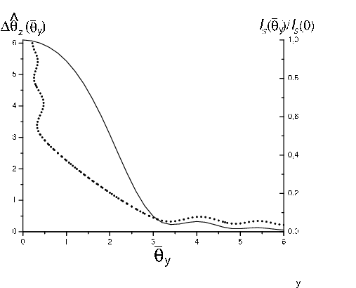
It should be noted that Eq. (269) does not depend on parameters and is, in fact, a universal function. Besides a geometrical factor ${\exp{[i2\bar{\theta}_{y}\hat{z}_{o}\Delta\hat{\theta}_{y}]}}$, the function $\chi$ represents the spectral degree of coherence in the vertical direction, once the horizontal coordinates are fixed. The fact that it is a universal function means that even in the case of zero vertical emittance we never have full coherence in the vertical direction. On the one hand, this phenomenon can be seen to be an influence of the presence of horizontal emittance on the vertical coherence properties of the photon beam, as the integral in $d\hat{\phi}_{x}$ in $\chi$ comes from an integration over the horizontal electron beam distribution. On the other hand, being $\chi$ a universal function, the influence of the horizontal emittance on the vertical coherence does not depend, in the limit for $\hat{N}_{x}\gg 1$ and $\hat{D}_{x}\gg 1$, on the actual values of $\hat{N}_{x}$ and $\hat{D}_{x}$. It is straightforward to see that $\chi$ is symmetric with respect to $\Delta\hat{\theta}_{y}$ and with respect to the exchange of $\Delta\hat{\theta}_{y}$ with $\bar{\theta}_{y}$. When $\bar{\theta}_{y}=0$, i.e. $\hat{\theta}_{y1}=-\hat{\theta}_{y2}$, we obviously obtain $\chi(0,\Delta\hat{\theta}_{y})=1$ that corresponds to complete coherence. In Fig. 25 we plot the three-dimensional representation of $\chi(\bar{\theta}_{y},\Delta\hat{\theta}_{y})$. In order to get a feeling for the behavior of $\chi$ we also plot, in Fig. 26 and Fig. 27, two cuts of Fig. 25 illustrating, respectively, the behavior of $\chi$ for a fixed $\bar{\theta}_{y}=0.5$ (or fixed $\Delta\hat{\theta}_{y}=0.5$) and at $\bar{\theta}_{y}=\Delta\hat{\theta}_{y}$.

As it is evident from Fig. 25, $\chi$ exhibits, for any fixed value of $\Delta\hat{\theta}_{y}$, many different zeros in $\bar{\theta}_{y}$. In Fig. 28 we illustrate some of these zeros as a function of $\Delta\hat{\theta}_{y}$, $\bar{\theta}_{y,Z}(\Delta\hat{\theta}_{y})$. The interest of this plot is that, once a certain distance $\hat{z}_{o}\Delta\hat{\theta}_{y}$ between two pinholes is fixed, it illustrates at what position of the pinhole system, $\bar{\theta}_{y,Z}$, the spectral degree of coherence drops from unity to zero for the first time.

It is interesting to compare Fig. 28, with the directivity diagram of the radiant intensity $I_{S}(\bar{\theta}_{y})$. This comparison is shown in Fig. 29. In the limit for $\hat{N}_{y}\ll 1$ and $\hat{D}_{y}\ll 1$, one may increase the degree of coherence of the beam by spatially filtering the radiation in the far field. If a vertical slit is used with aperture $d$ much larger than the horizontal coherence length, i.e. $d\gg\hat{\xi}_{cx}$, one would have poor coherence. Decreasing the aperture of the slit will increase the coherence of the X-ray beam up to some value $d$ smaller than $\hat{\xi}_{c}$. Within our assumption $\hat{N}_{x}\gg 1$ one has the far field approximation $\hat{\xi}_{cx}=(\pi/\hat{N}_{x})^{1/2}\hat{z}_{o}$. When $d$ becomes smaller and smaller with respect to $(\pi/\hat{N}_{x})^{1/2}\hat{z}_{o}$ the spectral degree of coherence $g$ can be identified with the universal function $\chi$, as once can see by inspecting Eq. (266). As a result, as $d$ becomes smaller one loses photons, but the X-ray beam transverse coherence ceases to improve because, as is seen in Fig. 29, the transverse degree of coherence $g=\chi$ drops to zero along the vertical radiation pattern of the filtered X-ray beam: for instance, from Fig. 29 one can see that $\chi$ drops to zero for the first time at $\Delta\hat{\theta}\sim 1$ $\bar{\theta}_{y}\sim 2$, where the X-ray flux is still intense. This behavior of the degree of coherence should be taken into account at the stage of planning experiments. To give an example, after spatial filtering, one may conduct a two-pinhole experiment (like the one illustrated in Fig. 7) and find, surprisingly, that for some vertical position $\bar{\theta}_{y}$ of the pinholes (at fixed $\Delta\hat{\theta}_{y}$) well within the radiation pattern diagram he will have no fringes, but for some other vertical position he can find perfect visibility. So, without the knowledge of the function $\chi$ a user would not even have the possibility to predict the outcomes of a simple two-pinhole experiment.

From the definitions of $\chi$, $\beta$, $\gamma$ and $I_{S}$ it can be seen that all universal functions introduced in this work are partial cases of the more generic

$$M(\bar{\theta}_{y},\Delta\hat{\theta}_{y})={\int_{-\infty}^{\infty}d\hat{\phi}_{x}\mathrm{sinc}{\left[\frac{\hat{\phi}_{x}^{2}+(\bar{\theta}_{y}-\Delta\hat{\theta}_{y})^{2}}{4}\right]}\mathrm{sinc}{\left[\frac{\hat{\phi}_{x}^{2}+(\bar{\theta}_{y}+\Delta\hat{\theta}_{y})^{2}}{4}\right]}}~.$$ (270)

In fact

$$\chi(\bar{\theta}_{y},\Delta\hat{\theta}_{y})=\frac{M(\bar{\theta}_{y},\Delta\hat{\theta}_{y})}{\left[M(\bar{\theta}_{y}+\Delta\hat{\theta}_{y},0)\right]^{1/2}\left[M(\bar{\theta}_{y}-\Delta\hat{\theta}_{y},0)\right]^{1/2}}$$ (271)

$$I_{S}(\bar{\theta}_{y})=M(\bar{\theta}_{y},0)$$ (272)

$$\beta(\Delta\hat{\theta}_{y})=\frac{1}{2\pi^{2}}\int_{-\infty}^{\infty}d\xi M(\xi,\Delta\hat{\theta}_{y})$$ (273)

$$\gamma(x)=\frac{1}{2\pi^{2}}\int_{-\infty}^{\infty}d\xi\exp[-i(2x)\xi]M(\xi,0)~.$$ (274)

Figure 30: Three-dimensional representation of $M$ as a function of $\bar{\theta}_{y}$ and $\Delta\hat{\theta}_{y}$.

The knowledge of $M$ is all one needs to calculate coherence properties out of many experimental setups, in very practical situations. It is therefore worth to tabulate $M$. We present a 3D plot of $M$, obtained from such tabulation, in Fig. 30.

Finally, it is interesting to sum up and compare results for the far field region obtained in this Section (non-homogeneous undulator source) with results obtained in Section 5. Many users performing coherent experiments with X-ray beams are interested in the beam coherence properties in the far field. We have seen that in the most general situation for third generation light sources one is interested in the case $\hat{N}_{x}\gg 1$ and $\hat{D}_{x}\gg 1$, which guarantees factorization of results in the $x$ and $y$ direction, with arbitrary $\hat{N}_{y}$ and $\hat{D}_{y}$. In this case we will not have, in general, weakly quasi-homogeneous radiation in the vertical direction. The spectral degree of coherence can be found by simplifying Eq. (128) in the mathematical limit $\hat{z}_{o}\longrightarrow\infty$:

$$g(\hat{z}_{o},\bar{\theta}_{x},\bar{\theta}_{y},\Delta\hat{\theta}_{x},\Delta\hat{\theta}_{y})={\exp{\left[i2\left(\bar{\theta}_{x}\hat{z}_{o}\Delta\hat{\theta}_{x}+\bar{\theta}_{y}\hat{z}_{o}\Delta\hat{\theta}_{y}\right)\right]}}$$ (275)

$$\times\exp{\left[-2\hat{N}_{x}\Delta\hat{\theta}_{x}^{2}\right]}\exp{\left[-2\hat{N}_{y}\Delta\hat{\theta}_{y}^{2}\right]}\int_{-\infty}^{\infty}d\hat{\phi}_{y}\exp{\left[-\frac{(\bar{\theta}_{y}+\hat{\phi}_{y})^{2}}{2\hat{D}_{y}}\right]}M(\hat{\phi}_{y},\Delta\hat{\theta}_{y})$$ (276)

$$\times\left\{\int_{-\infty}^{\infty}d\hat{\phi}_{y}\exp{\left[-\frac{(\hat{\phi}_{y}+\bar{\theta}_{y}+\Delta\hat{\theta}_{y})^{2}}{2\hat{D}_{y}}\right]}I_{S}(\hat{\phi}_{y})\right\}^{-1/2}$$ (277)

$$\times\left\{\int_{-\infty}^{\infty}d\hat{\phi}_{y}\exp{\left[-\frac{(\hat{\phi}_{y}+\bar{\theta}_{y}-\Delta\hat{\theta}_{y})^{2}}{2\hat{D}_{y}}\right]}I_{S}(\hat{\phi}_{y})\right\}^{-1/2}~.$$ (278)

We can see that for any value of $\hat{N}_{y}$ and $\hat{D}_{y}$, in the far field limit we obtain a contribution to the cross-spectral density for the $x$ and for the $y$ direction. The contribution for the $y$ direction can be expressed in terms of the product of an exponential function and convolutions between the (Gaussian) electron beam divergence and universal functions.

On the one hand, as $\hat{D}_{y}\ll 1$ we have

$$g(\hat{z}_{o},\bar{\theta}_{x},\bar{\theta}_{y},\Delta\hat{\theta}_{x},\Delta\hat{\theta}_{y})={\exp{\left[i2\left(\bar{\theta}_{x}\hat{z}_{o}\Delta\hat{\theta}_{x}+\bar{\theta}_{y}\hat{z}_{o}\Delta\hat{\theta}_{y}\right)\right]}}$$ (279)

$$\times\exp{\left[-2\hat{N}_{x}\Delta\hat{\theta}_{x}^{2}\right]}\exp{\left[-2\hat{N}_{y}\Delta\hat{\theta}_{y}^{2}\right]}\chi(\bar{\theta}_{y},\Delta\hat{\theta}_{y})~.$$ (280)

On the other hand, as $\hat{D}_{y}\gg 1$ we have weakly quasi-homogeneous wavefronts and

$$g(\hat{z}_{o},\bar{\theta}_{x},\bar{\theta}_{y},\Delta\hat{\theta}_{x},\Delta\hat{\theta}_{y})={\exp{\left[i2\left(\bar{\theta}_{x}\hat{z}_{o}\Delta\hat{\theta}_{x}+\bar{\theta}_{y}\hat{z}_{o}\Delta\hat{\theta}_{y}\right)\right]}}$$ (281)

$$\times\exp{\left[-2\hat{N}_{x}\Delta\hat{\theta}_{x}^{2}\right]}\exp{\left[-2\hat{N}_{y}\Delta\hat{\theta}_{y}^{2}\right]}\beta(\Delta\hat{\theta}_{y})~$$ (282)

where $\beta(\Delta\hat{\theta}_{y})$ is given in Eq. (191).

Moreover, as $\hat{N}_{y}\gg 1$, and for arbitrary $\hat{D}_{y}$ we have:

$$g(\hat{z}_{o},\bar{\theta}_{x},\bar{\theta}_{y},\Delta\hat{\theta}_{x},\Delta\hat{\theta}_{y})={\exp{\left[i2\left(\bar{\theta}_{x}\hat{z}_{o}\Delta\hat{\theta}_{x}+\bar{\theta}_{y}\hat{z}_{o}\Delta\hat{\theta}_{y}\right)\right]}}$$ (283)

$$\times\exp{\left[-2\hat{N}_{x}\Delta\hat{\theta}_{x}^{2}\right]}\exp{\left[-2\hat{N}_{y}\Delta\hat{\theta}_{y}^{2}\right]}~.$$ (284)

It should be noted that Eq. (284) is simply a consequence of the application of the VCZ theorem in both horizontal and vertical directions.

7 Application: Coherent X-ray beam expander scheme

In this Section we show how transverse coherence properties of an X-ray beam can be manipulated to obtain a larger coherent spot-size on a sample.

The idea of increasing the horizontal width of the coherence spot is based on the use of a downstream slit for selection of the transversely coherent fraction of undulator radiation. Imagine a slit very close to the exit of the undulator with an aperture $d$ comparable with the coherent length of the radiation at the exit of the undulator $\hat{\xi}_{cx}=\sqrt{\pi/\hat{D}_{x}}$, as illustrated in Fig. 31. The new radiation source after the slit is now coherent and characterized by a horizontal dimension of the light spot equal to $\sqrt{\pi/\hat{D}_{x}}$. In the far field one can take advantage of the reciprocal width relations of Fourier transform pairs or, equivalently, the expression for the Fraunhoffer diffraction pattern from a slit, i.e. a $\mathrm{sinc}$ function, to calculate the magnitude of the coherence spot. There is, of course, some arbitrary convention to agree upon when it comes to the definition of the width of the $\mathrm{sinc}$ function but, numerical factors aside, this reasoning shows qualitatively that the coherence spot is of order $\sqrt{\hat{D}_{x}}\hat{z}_{o}$ which is $\hat{\epsilon}_{x}$ times larger than the spot size dimension in the case of free-space propagation, of order $\hat{z}_{o}/\sqrt{\hat{N}_{x}}$. The radiation beyond the slit must be then spectrally filtered by a monochromator (not shown in Fig. 31) to further narrow the spectral bandwidth. Here we assume that the radiation frequency $\omega$ is equal to the fundamental frequency $\omega_{o}$. The radiation beyond the slit is transversely coherent when the aperture $d$ is equal (at most) to the coherence length $\xi_{cx}$.

Let us present a numerical example illustrating the improvement of the horizontal coherence length obtained by slit application. Let us consider the case when the electron horizontal emittance is large $\hat{\epsilon}_{x}\gg 1$ and the vertical emittance is small $\hat{\epsilon}_{y}\ll 1$, with $\hat{N}_{x}\gg\hat{D}_{x}$. Since $\hat{N}_{x}=\hat{\epsilon}_{x}\hat{\beta}_{x}$ and $\hat{D}_{x}=\hat{\epsilon}_{x}/\hat{\beta}_{x}$, this is the case, for instance when $\hat{\beta}_{x}\simeq 10$. Then, for $\hat{\epsilon}_{x}=100$ we have $\hat{N}_{x}=1000$ and $\hat{D}_{x}=10$. This particular numerical example has been considered in Section 4.1 to illustrate, in free space, the behavior of the coherence length as a function of the position along the beamline, given in Eq. (105). Suppose we install the slit at $\hat{z}_{o}=2$. From Eq. (105) we have $\hat{\xi}_{cx\mid\hat{z}_{o}=2}\sim\sqrt{\pi/\hat{D}_{x}}\sim 0.6$. At $\hat{z}_{o}=12$ we have a situation close to the asymptotic behavior where the field diffracted by the slit can be treated in the Fraunhofer approximation and $\hat{\xi}_{cx\mid\hat{z}_{o}=12}\sim\sqrt{\hat{D}_{x}}\hat{z}_{o}\sim 30$. Comparison of the asymptotic behaviors after spatial filtering with respect to the free-space propagation case is given in Fig. 32. Note that only the asymptotic behaviors near the slit and at large distance $\hat{z}_{o}\gg 1$ are plotted for the spatially filtered radiation. What is important is, in fact, the comparison between the coherent distance at large values of $\hat{z}_{o}$ with and without spatial filtering in the near zone.

This is an example in which evolution of transverse coherence through the beam line plays an important role. In fact, the ability of spatially filter radiation by a slit requires the knowledge of the transverse coherence length variation along the beamline.

Figure 31: Undulator radiation with a coherent X-ray beam expander.

Figure 32: Behavior of the horizontal coherence length as a function of distance for free space (dashed line) and comparison with asymptotic behaviors near the slit and at large distances (solid lines).

Let us calculate the number of coherent photons observed beyond the aperture. In the region of parameters where $\hat{N}_{x}\gg 1$ and $\hat{D}_{x}\gg 1$, the number of transversely coherent photons into the slit aperture $d=\xi_{cx}$ can be calculated as

$$(N_{\mathrm{ph}})_{\mathrm{coh}}=\frac{dN_{\mathrm{ph}}}{dx}\xi_{cx}~.$$ (285)

In the near-zone limit the slit is positioned at a position down the beamline $z_{s}\simeq\beta_{x}$ so that, from Eq. (105) and Eq. (89) we have:

$$\frac{dN_{\mathrm{ph}}}{dx}=\frac{N_{\mathrm{ph}}}{\sqrt{2\pi\sigma_{x}^{2}}}~$$ (286)

and

$$\xi_{cx}={\sqrt{\pi}}\frac{\lambda}{2\pi\sigma_{x^{\prime}}}~.$$ (287)

Therefore we can write

$$\frac{dN_{\mathrm{ph}}}{dx}\xi_{cx}={\sqrt{\pi}}\frac{\lambda N_{\mathrm{ph}}}{\sqrt{(2\pi)^{3}\sigma_{x}^{2}\sigma_{x^{\prime}}^{2}}}~.$$ (288)

At the opposite extreme, with the distance $z_{s}$ much larger than $\beta_{x}$ we find that, always from Eq. (105) and Eq. (89)

$$\frac{dN_{\mathrm{ph}}}{dx}=\frac{N_{\mathrm{ph}}}{\sqrt{2\pi z_{s}^{2}\sigma_{x^{\prime}}^{2}}}$$ (289)

and

$$\xi_{cx}={\sqrt{\pi}}\frac{\lambda z_{s}}{2\pi\sigma_{x}}~.$$ (290)

Therefore we can write

$$\frac{dN_{\mathrm{ph}}}{dx}\xi_{cx}={\sqrt{\pi}}\frac{\lambda N_{\mathrm{ph}}}{\sqrt{(2\pi)^{3}\sigma_{x}^{2}\sigma_{x^{\prime}}^{2}}}~.$$ (291)

Thus, the number of transversely coherent photons into the slit aperture $d=\xi_{cx}$ will be independent of the distance $z_{s}$. This means that operation of spatial filtering in the near field region, as proposed by us, will not diminish the number of coherent photons with respect to the usual practice in which spatial filtering to obtain coherent radiation is performed in the far field: its effect will only be that of increasing the horizontal dimension of the coherent spot size. This possibility to create transversely coherent radiation with large divergence in the horizontal direction is important for many experiments. The distance of the slit from the exit of the undulator sets a limit to achievable linear dimension of coherence area. If we build a coherent X-ray beam line, we want to have large linear dimension of coherence area at the specimen position. Therefore, in order to have a largest linear dimension of coherence area at the specimen position $\xi_{cx}(z_{o})\simeq\sigma_{x^{\prime}}z_{o}$ we must have a slit aperture of at most of the size $d\simeq\lambda/(2\pi\sigma_{x^{\prime}})$ installed in the near zone at $z_{s}\simeq\beta_{x}$. In order not to loose coherent photons instead, the slit aperture must be at least of the size $d\simeq\lambda/(2\pi\sigma_{x^{\prime}})$. The right compromise is thus a slit aperture of the size $d\simeq\lambda/(2\pi\sigma_{x^{\prime}})$ installed in the near zone at $z_{s}\simeq\beta_{x}$.

8 Conclusions

Before this work, no satisfactory theory describing spatial coherence from undulator radiation sources has been built. In this paper we developed such a theory of transverse coherence dealing with X-ray beams, with particular attention to third generation light sources.

First we studied Synchrotron Radiation as a random statistical process using the language of Statistical Optics. Statistical Optics developed around Gaussian, stationary processes characterized by quasi-homogeneous sources; under these assumptions, the characterization of statistical properties of the process are greatly simplified and the van Cittert-Zernike theorem (or its generalized version) can be used in order to describe the X-ray beam partial coherence properties in the far field region. However, for Synchrotron Radiation, there is no a priori reason to hold these assumptions satisfied.

We showed that Synchrotron Radiation is a Gaussian random process. As a result, statistical properties of Synchrotron Radiation are described satisfactory by second-order field correlation functions. We used a frequency domain analysis to describe them from a mathematical viewpoint. This choice is very natural. In fact, up-to-date detectors are limited to about $100$ ps time resolution: therefore, in real-life experiments with third generation light sources, detectors are by no means able to resolve a single X-ray pulse in time domain and work, instead, by counting the number of photons at a certain frequency over an integration time longer than the radiation pulse. As a consequence of the frequency domain analysis we could study the spatial correlation for a given frequency content using the cross-spectral density of the system which, independently of the spectral correlation function, can be used to extract useful information even if the process is not stationary.

We gave an expression for the process cross-spectral density dependent on six dimensionless parameters. Subsequently we tuned parameters at perfect resonance, thus obtaining a simplified expression.

First we studied the limit of applicability of the quasi-homogeneous model from an analytical viewpoint, within the framework of simplifying assumptions, namely in the limit of small electron beam divergence and Fresnel number in the vertical direction, of large electron beam divergence and Fresnel number in the horizontal direction, and performing calculations for the cross-spectral density on the horizontal plane only. This simplified study allowed us to introduce the concept of weakly quasi-homogeneous radiation and virtual quasi-homogeneous source while discussing the applicability region of the VCZ theorem.

Second, we studied the effect of the vertical emittance on the cross-spectral density. This study led us to analyze both cases in which the sources are weakly quasi-homogeneous and cases when they are not quasi-homogeneous at all. In the limit for large horizontal beam divergence and Fresnel number, which is always satisfied for third generation light sources, we found that the spectral degree of coherence factorizes in the product of factors depending separately on the horizontal and on the vertical coordinates. In the far field limit the vertical part of the spectral degree of coherence can be expressed in terms of the product of an exponential function (which, alone, would simply satisfy the VCZ theorem) and convolutions between the electron beam divergence in the vertical direction and a universal functions, that we introduced in our work. The universality of such a function implied that even for zero vertical emittance we never have full coherence in the vertical direction. This unexpected result is due to the influence of the horizontal emittance on the vertical coherence properties of the photon beam. Because of this, the degree of coherence changes between zero and unity within the diffraction angle. We also studied the near field zone. When one is interested in the evolution of the degree of coherence along the beamline back up to the exit of the undulator the situation becomes much more complicated with respect to the far zone case, as the observation distance is one of the problem parameters. There are many more asymptotic situations which can be studied, and a large part of our paper is devoted to the calculation of these asymptotic situations. We provided approximate estimations for the vertical coherence length that are valid from the far zone and back, up to the exit of the undulator in the case when either the vertical Fresnel number or the vertical electron beam divergence are much larger than unity. These can be used at the stage of planning experiments.

It should be noted that, throughout this work, we did not discuss the accuracy of the approximation of small and large parameters. In order to do so, one needs to develop a perturbation theory for each asymptotic case studied here, which would considerably increase the size of this paper. As a result we leave this issue for future work.

Finally, we selected an application to show the power of our approach. We discussed how the transverse coherence properties of an X-ray beam can be manipulated to obtain a convenient coherent spot-size on the sample with the help of a simple vertical slit; this invention was predicted almost entirely on the basis of theoretical ideas of rather complex and abstract nature discussed in the previous parts of the paper.

Appendix A: Random phasor sum

The field of thermal light can be regarded as a sum of a great many independent contributions. The complex envelope of polarized thermal light at fixed time and a fixed point in space is a sum of a very large number of complex phasors

$$E(\vec{r},t)=\sum_{k=1}^{N}\alpha_{k}e^{i\psi_{k}}~,$$ (292)

where $N$ is the number of radiating atoms. Statistical properties of elementary phasors that are generally satisfied in thermal light problems of interest are as follows:

a) The amplitudes $\alpha_{k}=Re(\alpha_{k})$ and the phases $\psi_{k}$ are statistically independent of each other and of the amplitudes and phases of all other elementary phases for different values of $k$.

b) The random variables $\alpha_{k}$ are identically distributed for all $k$ with mean value $<\alpha>$ and second moment $<\alpha^{2}>$.

c) The phases $\psi_{k}$ are uniformly distributed over the interval $(0,2\pi)$.

The reader can find in [5] that when assumptions from a) to c) are satisfied, the real ($Re(E)$) and imaginary ($Im(E)$) parts of the field are distributed in accordance with the Gaussian law in the limit for $N\longrightarrow\infty$, so that

$$\left\langle Re(E)\right\rangle=\left\langle Im(E)\right\rangle=0~,$$ (293)

$$\left\langle[Re(E)]^{2}\right\rangle=\left\langle[Im(E)]^{2}\right\rangle=\frac{\left\langle\alpha^{2}\right\rangle}{2}N=\sigma^{2}~,$$ (294)

$$\left\langle Re(E)Im(E)\right\rangle=0~,$$ (295)

$$p(Re(E),Im(E))=\frac{1}{2\pi\sigma^{2}}\exp{\left[-\frac{[Re(E)]^{2}+[Im(E)]^{2}}{2\sigma^{2}}\right]}~,$$ (296)

where $p(Re(E),Im(E))$ is the joint probability density function.

In Section 2.1 we discussed statistical properties of Synchrotron Radiation and we were led to assumptions 1), 2) and 3) which are weaker than a), b) and c). Here we will demonstrate that assumptions from a) to c) can be relaxed to assumptions from 1) to 3) without changes in results. We will derive results valid when the amplitudes $\alpha_{k}$ are complex $\alpha_{k}=|\alpha_{k}|\exp{(i\phi_{k})}$.

After denoting with $r$ and $i$ the real and imaginary parts of the fields and after substituting notation $\langle Q\rangle$ with $\bar{Q}$ we first demonstrate that $\bar{r}=\bar{i}=0$. We have straightforwardly

$$\bar{r}=\frac{1}{N}\sum_{k=1}^{N}\Bigg(\overline{\mid\alpha_{k}\mid\cos\phi_{k}}~{\overline{\cos\psi_{k}}}-\overline{\mid\alpha_{k}\mid\sin\phi_{k}}~\overline{\sin\psi_{k}}\Bigg)=0~,$$ (297)

$$\bar{i}=\frac{1}{N}\sum_{k=1}^{N}\Bigg(\overline{\mid\alpha_{k}\mid\cos\phi_{k}}~\overline{\sin\psi_{k}}+\overline{\mid\alpha_{k}\mid\sin\phi_{k}}~\overline{\cos\psi_{k}}\Bigg)=0~,$$ (298)

because all averages over trigonometric functions are zero.

Second, we demonstrate that $\overline{r^{2}}=\overline{i^{2}}=\overline{\alpha^{2}}/2$. Again, direct calculation shows

$$\bar{r^{2}}=\frac{1}{N}\sum_{k,n=1}^{N}\Bigg({\overline{\mid\alpha_{k}\mid\mid\alpha_{n}\mid\cos\phi_{k}\cos\phi_{n}}}~{\overline{\cos\psi_{k}\cos\psi_{n}}}$$ (299)

$$+{\overline{\mid\alpha_{k}\mid\mid\alpha_{n}\mid\sin\phi_{k}\sin\phi_{n}}}~{\overline{\sin\psi_{k}\sin\psi_{n}}}$$ (300)

$$-{\overline{\mid\alpha_{k}\mid\mid\alpha_{n}\mid\cos\phi_{k}\sin\phi_{n}}}~{\overline{\cos\psi_{k}\sin\psi_{n}}}$$ (301)

$$-{\overline{\mid\alpha_{k}\mid\mid\alpha_{n}\mid\sin\phi_{k}\cos\phi_{n}}}~{\overline{\sin\psi_{k}\sin\psi_{n}}}\Bigg)$$ (302)

$$=\frac{1}{2N}\sum_{k=1}^{N}\overline{\mid\alpha_{k}\mid^{2}\left(\cos^{2}\psi_{k}+\sin^{2}\psi_{k}\right)}=\frac{\overline{\alpha^{2}}}{2}~.$$ (303)

Moreover it is easy to see that $\overline{i^{2}}=\overline{r^{2}}$.

Finally, we show that $\overline{ri}=0$. In fact

$$\overline{ri}=\frac{1}{N}\sum_{k,n=1}^{N}\Bigg(\overline{\mid\alpha_{k}\mid\mid\alpha_{n}\mid\cos\phi_{k}\cos\phi_{n}}~{\overline{\cos\psi_{k}\sin\psi_{n}}}$$ (304)

$$+\overline{\mid\alpha_{k}\mid\mid\alpha_{n}\mid\cos\phi_{k}\sin\phi_{n}}~{\overline{\cos\psi_{k}\cos\psi_{n}}}$$ (305)

$$-\overline{\mid\alpha_{k}\mid\mid\alpha_{n}\mid\sin\phi_{k}\cos\phi_{n}}~{\overline{\sin\psi_{k}\sin\psi_{n}}}$$ (306)

$$-\overline{\mid\alpha_{k}\mid\mid\alpha_{n}\mid\sin\phi_{k}\sin\phi_{n}}~{\overline{\sin\psi_{k}\cos\psi_{n}}}\Bigg)$$ (307)

$$=\frac{1}{2N}\sum_{k}\overline{{|\alpha_{k}|^{2}}\left({{\cos\phi_{k}\sin\phi_{k}}}-{{\sin\phi_{k}\cos\phi_{k}}}\right)}=0~.$$ (308)

As a result we have that real and imaginary parts have zero means, equal variances and are uncorrelated. Use of the central limit theorem allows to conclude that the resulting phasor sum is a circular complex Gaussian random variable.

Appendix B: A useful transformation of the expression for the undulator radiation field

We start reporting here, for convenience, Eq. (39), that represents the field (in normalized units) produced by a particle with offset and deflection at any distance $\hat{z}_{o}\geqslant 1/2$ from the exit of the undulator, where the undulator center is taken at $\hat{z}_{o}=0$:

$$\hat{E}_{s\bot}=\hat{z}_{o}\int_{-1/2}^{1/2}d\hat{z}^{\prime}\frac{1}{\hat{z}_{o}-\hat{z}^{\prime}}\exp\left\{i\left[\left(\hat{C}+\frac{\left.\vec{\hat{\eta}}\right.^{2}}{2}\right)\hat{z}^{\prime}+\frac{\left(\vec{\hat{{r}}}_{\bot o}-\vec{{\hat{l}}}-\vec{\hat{\eta}}\hat{z}^{\prime}\right)^{2}}{2(\hat{z}_{o}-\hat{z}^{\prime})}\right]\right\}.~$$ (309)

In this Appendix we show that $\hat{E}_{s\bot}$ as reported in Eq. (309) may be described as

$$\hat{E}_{s\bot}=\int_{-1/2}^{1/2}\frac{\hat{z}_{o}d\hat{z}^{\prime}}{\hat{z}_{o}-\hat{z}^{\prime}}\exp\left\{i\left[\Phi_{U}+\hat{C}\hat{z}^{\prime}+\frac{\hat{z}_{o}\hat{z}^{\prime}}{2(\hat{z}_{o}-\hat{z}^{\prime})}\left(\vec{\hat{\theta}}-\frac{\vec{\hat{l}}}{\hat{z}_{o}}-\vec{\hat{\eta}}\right)^{2}\right]\right\}$$ (310)

where $\Phi_{U}$ is given by

$$\Phi_{U}=\left[\left(\hat{\theta}_{x}-\frac{\hat{l}_{x}}{\hat{z}_{o}}\right)^{2}+\left(\hat{\theta}_{y}-\frac{\hat{l}_{y}}{\hat{z}_{o}}\right)^{2}\right]\frac{\hat{z}_{o}}{2}~.$$ (311)

This means that $\hat{E}_{s\bot}$ is of the form

$$\hat{E}_{s\bot}\left(\hat{C},\hat{z}_{o},\vec{\hat{\theta}}-(\vec{\hat{l}}/\hat{z}_{o})-\vec{\hat{\eta}}\right)=\exp({i\Phi_{U}})S\left(\hat{C},\hat{z}_{o},\vec{\hat{\theta}}-(\vec{\hat{l}}/\hat{z}_{o})-\vec{\hat{\eta}}\right)~.$$ (312)

Let us introduce in this Appendix, for simplicity of notation, $\vec{\hat{\xi}}=\vec{\hat{{r}}}_{\bot o}-\vec{{\hat{l}}}$ and $\vec{\hat{\phi}}=\vec{\xi}/\hat{z}_{o}$. It is easy to rewrite the phase in the integrand of Eq. (309), which we denote with $\Phi_{T}$ as

$$\Phi_{T}=\hat{C}\hat{z}^{\prime}+\frac{\left.\vec{\hat{\eta}}\right.^{2}}{2}\hat{z}^{\prime}+\frac{1}{2}\left\{\left[\vec{\hat{\phi}}^{2}\hat{z}_{o}-2\vec{\hat{\phi}}\cdot\vec{\hat{\eta}}\hat{z}^{\prime}+\frac{\vec{\hat{\eta}}^{2}\hat{z}^{\prime 2}}{\hat{z}_{o}}\right]\left[1+\sum_{n=1}^{\infty}\left(\frac{\hat{z}^{\prime}}{\hat{z}_{o}}\right)^{n}\right]\right\}~.$$ (313)

Further algebraic manipulation of Eq. (313) yields

$$\Phi_{T}=\hat{C}\hat{z}^{\prime}+\frac{\vec{\hat{\phi}}^{2}\hat{z}_{o}}{2}+\frac{\hat{z}^{\prime}}{2}\left(\vec{\hat{\phi}}-\vec{\hat{\eta}}\right)^{2}+\frac{1}{2}\left\{\frac{\vec{\hat{\eta}}^{2}\hat{z}^{\prime 2}}{\hat{z}_{o}}+\frac{\vec{\hat{\eta}}^{2}\hat{z}^{\prime 2}}{\hat{z}_{o}}\sum_{n=1}^{\infty}\left(\frac{\hat{z}^{\prime}}{\hat{z}_{o}}\right)^{n}\right.$$ (314)

$$\left.+\vec{\hat{\phi}}^{2}\hat{z}_{o}\sum_{n=2}^{\infty}\left(\frac{\hat{z}^{\prime}}{\hat{z}_{o}}\right)^{n}-2\vec{\hat{\phi}}\cdot\vec{\hat{\eta}}\hat{z}^{\prime}\sum_{n=1}^{\infty}\left(\frac{\hat{z}^{\prime}}{\hat{z}_{o}}\right)^{n}\right\}~.$$ (315)

It is easy to recognize $\Phi_{U}$ in the second term on the right hand side of Eq. (315). Furthermore, the fourth term on the right hand side of Eq. (315) can be further manipulated, leading to

$$\Phi_{T}=\hat{C}\hat{z}^{\prime}+\Phi_{U}+\frac{\hat{z}^{\prime}}{2}\left(\vec{\hat{\phi}}-\vec{\hat{\eta}}\right)^{2}$$ (316)

$$+\frac{1}{2}\left\{\hat{z}_{o}\left(\vec{\hat{\phi}}^{2}+\vec{\hat{\eta}}^{2}\right)\sum_{n=2}^{\infty}\left(\frac{\hat{z}^{\prime}}{\hat{z}_{o}}\right)^{n}-2\vec{\hat{\phi}}\cdot\vec{\hat{\eta}}\hat{z}_{o}\sum_{n=2}^{\infty}\left(\frac{\hat{z}^{\prime}}{\hat{z}_{o}}\right)^{n}\right\}~,$$ (317)

that is

$$\Phi_{T}=\hat{C}\hat{z}^{\prime}+\Phi_{U}+\frac{\hat{z}^{\prime}}{2}\left(\vec{\hat{\phi}}-\vec{\hat{\eta}}\right)^{2}+\frac{\hat{z}_{o}}{2}\left\{\left(\vec{\hat{\phi}}-\vec{\hat{\eta}}\right)^{2}\sum_{n=2}^{\infty}\left(\frac{\hat{z}^{\prime}}{\hat{z}_{o}}\right)^{n}\right\}~$$ (318)

or

$$\Phi_{T}=\hat{C}\hat{z}^{\prime}+\Phi_{U}+\frac{\hat{z}_{o}\hat{z}^{\prime}}{2(\hat{z}_{o}-\hat{z}^{\prime})}\left(\vec{\hat{\phi}}-\vec{\hat{\eta}}\right)^{2}~$$ (319)

Therefore, since

$$\vec{\hat{\phi}}-\vec{\hat{\eta}}=\vec{\hat{\theta}}-\frac{\vec{\hat{l}}}{\hat{z}_{o}}-\vec{\hat{\eta}}~$$ (320)

we have

$$\hat{E}_{s\bot}=\int_{-1/2}^{1/2}\frac{\hat{z}_{o}d\hat{z}^{\prime}}{\hat{z}_{o}-\hat{z}^{\prime}}\exp\left\{i\left[\Phi_{U}+\hat{C}\hat{z}^{\prime}+\frac{\hat{z}_{o}\hat{z}^{\prime}}{2(\hat{z}_{o}-\hat{z}^{\prime})}\left(\vec{\hat{\theta}}-\frac{\vec{\hat{l}}}{\hat{z}_{o}}-\vec{\hat{\eta}}\right)^{2}\right]\right\}$$ (321)

that is Eq. (310), quantum erat demonstrandum.

Appendix C: Autocorrelation function for undulator sources

In this Appendix we demonstrate the validity of Eq. (188). Having defined

$$\tilde{f}(\hat{z}_{o},\Delta\hat{\theta}_{y})=\frac{1}{2\pi^{2}}\int_{-\infty}^{\infty}d\hat{\phi}_{y}\int_{-\infty}^{\infty}d\hat{\phi}_{x}S^{*}{\left[\hat{z}_{o},\hat{\phi}_{x}^{2}+(\hat{\phi}_{y}-\Delta\hat{\theta}_{y})^{2}\right]}S{\left[\hat{z}_{o},\hat{\phi}_{x}^{2}+(\hat{\phi}_{y}+\Delta\hat{\theta}_{y})^{2}\right]}~,~~~~~~$$ (322)

and

$$\beta(\Delta\hat{\theta}_{y})=\frac{1}{2\pi^{2}}\int_{-\infty}^{\infty}d\hat{\phi}_{y}\int_{-\infty}^{\infty}d\hat{\phi}_{x}\mathrm{sinc}{\left[\frac{\hat{\phi}_{x}^{2}+(\hat{\phi}_{y}-\Delta\hat{\theta}_{y})^{2}}{4}\right]}\mathrm{sinc}{\left[\frac{\hat{\phi}_{x}^{2}+(\hat{\phi}_{y}+\Delta\hat{\theta}_{y})^{2}}{4}\right]}~,~~~~~~$$ (323)

we have want to demonstrate that Eq. (188) holds, that is

$$\tilde{f}(\hat{z}_{o},\Delta\hat{\theta}_{y})=\beta(\Delta\hat{\theta}_{y})~.$$ (324)

The proof is based on the autocorrelation theorem, which states that if the (two-dimensional) Fourier Transform of a function $w(x,y)$ with respect to variables $\alpha_{x}$ and $\alpha_{y}$ is indicated by $\bar{w}(\alpha_{x},\alpha_{y})$, then the Fourier transform of the two-dimensional autocorrelation function of $w(x,y)$ with respect to the same variables $\alpha_{x}$ and $\alpha_{y}$ is given by $|\bar{w}(\alpha_{x},\alpha_{y})|^{2}$. In formulas, after definition of the autocorrelation function

$$\mathcal{A}[w](x,y)=\int_{-\infty}^{\infty}d\eta\int_{-\infty}^{\infty}d\xi w(\eta+x,\xi+y)w^{*}(\eta,\xi)~,$$ (325)

which is equivalent to

$$\mathcal{A}[w](x,y)=\int_{-\infty}^{\infty}d\eta\int_{-\infty}^{\infty}d\xi w(\eta+x/2,\xi+y/2)w^{*}(\eta-x/2,\xi-y/2)~,$$ (326)

the autocorrelation theorem states that

$$\int_{-\infty}^{\infty}dx\int_{-\infty}^{\infty}dy\exp{[i(\alpha_{x}x+\alpha_{y}y)]}\mathcal{A}[w](x,y)=|\bar{w}(\alpha_{x},\alpha_{y})|^{2}~.$$ (327)

First we extend the definition of $\tilde{f}$

$$\tilde{f}(\hat{z}_{o},\Delta\hat{\theta}_{x}^{\prime},\Delta\hat{\theta}_{y}^{\prime})=\frac{1}{2\pi^{2}}\int_{-\infty}^{\infty}d\hat{\phi}_{y}\int_{-\infty}^{\infty}d\hat{\phi}_{x}S^{*}{\left[\hat{z}_{o},(\hat{\phi}_{x}-\Delta\hat{\theta}_{x}^{\prime}/2)^{2}+(\hat{\phi}_{y}-\Delta\hat{\theta}_{y}^{\prime}/2)^{2}\right]}$$ (328)

$$\times S{\left[\hat{z}_{o},(\hat{\phi}_{x}+\Delta\hat{\theta}_{x}^{\prime}/2)^{2}+(\hat{\phi}_{y}+\Delta\hat{\theta}_{y}^{\prime}/2)^{2}\right]}~,~~~~~~$$ (329)

where we changed variables from $\Delta\hat{\theta}_{x,y}$ to $\Delta\hat{\theta}_{x,y}^{\prime}=2\Delta\hat{\theta}_{x,y}$ Then we can apply the autocorrelation theorem in Eq. (327) to the function $\tilde{f}$ thus obtaining the following relation:

$$\int_{-\infty}^{\infty}d\Delta\hat{\theta}_{x}^{\prime}\int_{-\infty}^{\infty}d\Delta\hat{\theta}_{y}^{\prime}\exp{[i(\alpha_{x}\Delta\hat{\theta}_{x}^{\prime}+\alpha_{y}\Delta\hat{\theta}_{y}^{\prime})]}\tilde{f}(\hat{z}_{o},\Delta\hat{\theta}_{x}^{\prime},\Delta\hat{\theta}_{y}^{\prime})$$ (330)

$$=\frac{1}{2\pi^{2}}\left|\int_{-\infty}^{\infty}d\hat{\phi}_{x}\int_{-\infty}^{\infty}d\hat{\phi}_{y}\exp{[i(\alpha_{x}\hat{\phi}_{x}+\alpha_{y}\hat{\phi}_{y})]}S{\left[\hat{z}_{o},\hat{\phi}_{x}^{2}+\hat{\phi}_{y}^{2}\right]}\right|^{2}~,$$ (331)

where $\alpha_{x,y}$ are now conjugated variables with respect to the angles $\hat{\phi}_{x,y}$ on which $S$ depends. We will denote with $\bar{S}$ the two-dimensional Fourier Transform of $S$, that is:

$$\bar{S}({\alpha}_{x},{\alpha}_{y})=\int_{-\infty}^{\infty}d\hat{\phi}_{x}\int_{-\infty}^{\infty}d\hat{\phi}_{y}\exp{[i(\alpha_{x}\hat{\phi}_{x}+\alpha_{y}\hat{\phi}_{y})]}S{\left[\hat{z}_{o},\hat{\phi}_{x}^{2}+\hat{\phi}_{y}^{2}\right]}~.$$ (332)

The relation between the function $S$ and the undulator field is given by Eq. (51), and one has

$$\bar{S}({\alpha}_{x},{\alpha}_{y})=\int_{-\infty}^{\infty}d\hat{\phi}_{x}\int_{-\infty}^{\infty}d\hat{\phi}_{y}\exp{[i(\alpha_{x}\hat{\phi}_{x}+\alpha_{y}\hat{\phi}_{y})]}\exp{[-i(\hat{\phi}_{x}^{2}+\hat{\phi}_{y}^{2})\hat{z}_{o}/2]}$$ (333)

$$\times\hat{E}_{s\bot}{\left[\hat{z}_{o},\hat{\phi}_{x}^{2}+\hat{\phi}_{y}^{2}\right]}~.$$ (334)

After definition of $\bar{\alpha}_{x,y}=\alpha_{x,y}/\hat{z}_{o}$ one can write $\bar{S}$, as a function of $\bar{\alpha}_{x,y}$ instead of $\alpha_{x,y}$. Then, one can switch to the new integration variables $\hat{x}=\hat{\phi}_{x}\hat{z}_{o}$ and $\hat{y}=\hat{\phi}_{y}\hat{z}_{o}$ to obtain:

$$\bar{S}(\bar{\alpha}_{x},\bar{\alpha}_{y})=\frac{1}{\hat{z}_{o}^{2}}\int_{-\infty}^{\infty}d\hat{x}\int_{-\infty}^{\infty}d\hat{y}\exp{[i(\bar{\alpha}_{x}\hat{x}+\bar{\alpha}_{y}\hat{y})]}\exp{[-i(\hat{x}^{2}+\hat{y}^{2})/(2\hat{z}_{o})]}$$ (335)

$$\times\hat{E}_{s\bot}{\left[\hat{z}_{o},\hat{x}^{2}+\hat{y}^{2}\right]}~.$$ (336)

(337)

where the expression for $\hat{E}_{s\bot}{[\hat{z}_{o},\hat{x}^{2}+\hat{y}^{2}]}$ is given in Eq. (39). Now we have to calculate the Fourier transform of the product of two factors: $\exp{[-i(\hat{x}^{2}+\hat{y}^{2})/(2\hat{z}_{o})]}$ and $\hat{E}_{\bot s}$. Let us look for the Fourier transform of each factor.

A direct calculation shows that

$$\int_{-\infty}^{\infty}d\hat{x}\int_{-\infty}^{\infty}d\hat{y}\exp{[i(\bar{\alpha}_{x}\hat{x}+\bar{\alpha}_{y}\hat{y})]}\hat{E}_{s\bot}\left(\hat{z}_{o},\hat{x}^{2}+\hat{y}^{2}\right)$$ (338)

$$=2i\pi\hat{z}_{o}\exp{\left[-i\frac{(\bar{\alpha}_{x}^{2}+\bar{\alpha}_{y}^{2})\hat{z}_{o}}{2}\right]}\mathrm{sinc}\left[\frac{\bar{\alpha}_{x}^{2}+\bar{\alpha}_{y}^{2}}{4}\right]~.$$ (339)

Second, let us deal with the Fourier transform of $\exp{[-i(\hat{x}^{2}+\hat{y}^{2})/(2\hat{z}_{o})]}$:

$$\int_{-\infty}^{\infty}d\hat{x}\int_{-\infty}^{\infty}d\hat{y}\exp{[i(\bar{\alpha}_{x}\hat{x}+\bar{\alpha}_{y}\hat{y})]}\exp{[-i(\hat{x}^{2}+\hat{y}^{2})/(2\hat{z}_{o})]}$$ (340)

$$=-4i\hat{z}_{o}\exp{[i(\bar{\alpha}_{x}^{2}+\bar{\alpha}_{y}^{2})\hat{z}_{o}/2]}~.$$ (341)

Since the Fourier transform of a product is equal to the convolution of the Fourier transforms of the factors we have

$$\bar{S}(\bar{\alpha}_{x},\bar{\alpha}_{y})=8\pi\int_{-\infty}^{\infty}du\int_{-\infty}^{\infty}dw\exp{\{i[(\bar{\alpha}_{x}-u)^{2}+(\bar{\alpha}_{y}-w)^{2}]\hat{z}_{o}/2\}}$$ (342)

$$\times\exp{[-i(u^{2}+w^{2})\hat{z}_{o}/2]}\mathrm{sinc}[(u^{2}+w^{2})/4]~.$$ (343)

and therefore we have

$$|\bar{S}(\bar{\alpha}_{x},\bar{\alpha}_{y})|=8\pi\left|\int_{-\infty}^{\infty}du\int_{-\infty}^{\infty}dw\exp{[i(\bar{\alpha}_{x}u+\bar{\alpha}_{y}w)\hat{z}_{o}]}\mathrm{sinc}[(u^{2}+w^{2})/4]\right|~.$$ (344)

Going back to old variables $\alpha_{x,y}$ we obtain

$$|\bar{S}({\alpha}_{x},{\alpha}_{y})|=8\pi\left|\int_{-\infty}^{\infty}du\int_{-\infty}^{\infty}dw\exp{[i({\alpha}_{x}u+{\alpha}_{y}w)]}\mathrm{sinc}[(u^{2}+w^{2})/4]\right|~.$$ (345)

which is independent of $\hat{z}_{o}$. As a result Eq. (331) is also independent on $\hat{z}_{o}$, i.e. the Fourier transform of $\tilde{f}$ is independent of $\hat{z}_{o}$.

Now, on the one hand in the limit for $\hat{z}_{o}\longrightarrow\infty$ the function $\tilde{f}$ transforms into $\beta$, because the $S$ functions in $\tilde{f}$ tend asymptotically to the $\mathrm{sinc}$ functions in $\beta$. On the other hand, if the Fourier transform of $\tilde{f}$ is independent of $\hat{z}_{o}$, also $\tilde{f}$ is independent of $\hat{z}_{o}$. As a result it can only be $\tilde{f}(\Delta\hat{\theta}_{y}^{\prime})=\beta(\Delta\hat{\theta}_{y}^{\prime})$, and $\tilde{f}(\Delta\hat{\theta}_{y})=\beta(\Delta\hat{\theta}_{y})$ that is Eq. (324) holds, quantum erat demonstrandum.

Note that, based on the autocorrelation theorem, it is also possible to give an analytic expression for the Fourier transform of $\beta$. After definition of $\beta=\beta(\hat{z}_{o},\Delta\hat{\theta}_{x}^{\prime},\Delta\hat{\theta}_{y}^{\prime})$ as in Eq. (329), application of the autocorrelation theorem simply states that the two-dimensional Fourier Transform of $\beta$, that will be indicated with $\bar{\beta}$ can be written as

$$\bar{\beta}(\alpha_{x},\alpha_{y})=\frac{1}{2\pi^{2}}\left|\int_{-\infty}^{\infty}d\hat{\phi}_{x}\int_{-\infty}^{\infty}d\hat{\phi}_{y}\exp{[i(\alpha_{x}\hat{\phi}_{x}+\alpha_{y}\hat{\phi}_{y})]}\mathrm{sinc}\left(\frac{\hat{\phi}_{x}^{2}+\hat{\phi}_{y}^{2}}{4}\right)\right|^{2}~.$$ (346)

Introducing $\alpha^{2}=\alpha_{x}^{2}+\alpha_{y}^{2}$ and representing the two-dimensional Fourier Transform of $\beta$ in terms of Fourier-Bessel transform we obtain

$$\bar{\beta}(\alpha)=\frac{1}{2\pi^{2}}\left|2\pi\int_{0}^{\infty}dr~rJ_{0}(r\alpha)\mathrm{sinc}\left(\frac{r^{2}}{4}\right)\right|^{2}=2\left[\pi-2\mathrm{Si}(\alpha^{2})\right]^{2}~,$$ (347)

where $\mathrm{Si}$ indicates the sine integral function.

Finally, one can get back a simpler representation of the function $\beta$ in terms of a one-dimensional integration simply performing an anti Fourier-Bessel transform:

$${\beta}(\Delta\hat{\theta}^{\prime})=\frac{1}{2\pi}\int_{0}^{\infty}d\alpha~\alpha J_{0}(\alpha\Delta\hat{\theta}^{\prime})\bar{\beta}(\alpha)~,$$ (348)

where $\Delta\hat{\theta}^{{}^{\prime}2}=\Delta\hat{\theta}_{x}^{{}^{\prime}2}+\Delta\hat{\theta}_{y}^{{}^{\prime}2}$. For $\Delta\hat{\theta}_{x}=0$ we obtain

$${\beta}(\Delta\hat{\theta}_{y})=\frac{1}{\pi}\int_{0}^{\infty}d\alpha~\alpha J_{0}\left(\alpha\frac{\Delta\hat{\theta}_{y}}{2}\right)\left[\pi-2\mathrm{Si}(\alpha^{2})\right]^{2}~.$$ (349)

References

- [1] PETRA III Technical Design Report, ISSN 0418-9833, edited by K. Balewski et al., DESY, Hamburg (2004)
- [2] C. Chang, P. Naulleau et al., Appied Optics, 14 (2003)
- [3] G. Geloni, E. Saldin, E. Schneidmiller and M. Yurkov, Paraxial Green’s functions in Synchrotron Radiation theory, DESY 05-032, ISSN 0418-9833 (2005)
- [4] Y. Takatama et al., Nucl. Instr. Meth. in Phys. Res. A 441, 565 (2000)
- [5] J. W. Goodman, Statistical Optics, John Wiley Sons, Inc., 1985
- [6] L. Mandel and E. Wolf, Optical Coherence and Quantum Optics, Cambridge University Press, 1995
- [7] D. Attwood, Soft X-rays and extreme ultraviolet radiation, Cambridge University Press, 1999
- [8] M. Yabashi, K. Tamasku et al., Phys. Rev. Lett., 88, 24 (2000)
- [9] E. Wolf, Nature, 172, 535 (1953)
- [10] E. O’Neill, Introduction to Statistical Optics, Dover Publications Inc., Mineola, New York (1991)