Nonlinear Magneto-Optical Rotation of Elliptically Polarized Light

Abstract

We predict theoretically and demonstrate experimentally an ellipticity-dependent nonlinear magneto-optic rotation of elliptically-polarized light propagating in a medium with atomic coherence. We show that this effect results from hexadecapole and higher order moments of the atomic coherence, and is associated with an enhancement of Kerr and higher orders nonlinearities accompanied by suppression of the other linear and nonlinear susceptibility terms of the medium. These nonlinearities might be useful for quantum signal processing. In particular, we report an observation of an enhancement of the polarization rotation of elliptically polarized light resonant with the $5S_{1/2}F=2\rightarrow 5P_{1/2}F=1$ transition of ⁸⁷Rb.

I Introduction

Nonlinear magneto-optic rotation (NMOR) of the polarization plane of light resonant with atomic transitions is attracting increasing attention [1, 2]. Ultranarrow (up to $1$ Hz [3, 4]) spectral features accompanied by strong polarization rotation observed in NMOR experiments are used (or proposed to be used) in sensitive magnetometry [5, 6, 7], in time-reversal-invariance violation experiments [8, 9, 10], in measurements of the electron dipole moment [11, 12], and in measurements of various atomic constants [13]. Extremely slow propagation of light has also been observed in NMOR in hot rubidium vapor [14].

The most accurate description of the properties of NMOR signals is obtained from an analysis of density matrix equations for the atomic polarizations and populations along with Maxwell equations describing propagation of the electromagnetic fields in the atomic medium. The exact solution of this problem, however, is very complicated, and for most cases may be obtained only numerically. The problem should be somehow simplified to obtain analytical results.

The traditional approach to solution of the problem is based on the approximation of weak electromagnetic fields and low atomic vapor densities [15, 16, 17, 18], conditions found in early experiments involving incoherent radiation from atomic discharge lamps. In this case one can use perturbation theory, and the atomic susceptibility may be decomposed in a series of the electromagnetic fields involved. Magnetic field dependent terms of the susceptibility decomposition which are nonlinear in the electromagnetic fields are responsible for NMOR. It can be demonstrated that only two-photon processes are important in this approximation, and therefore complicated multilevel systems may be reduced to systems with small level number (such as $\Lambda$, $V$, or $X$–schemes) [17, 19, 20]. In this approximation, NMOR is a consequence of low frequency ground-state coherence formed by two-photon processes between Zeeman sublevels with difference in magnetic quantum numbers equal to $\Delta m=\pm 2$.

In some cases it is convenient to describe the atom-light interaction from the point of view of light-induced multipole moments of the atomic electron distribution. Conventionally this is done in terms of an irreducible tensor representation of the density matrix [21, 22, 23]. In this case, the ground-state coherence is equivalent to the quadrupole moment, or alignment. It has been suggested that NMOR is a consequence of the alignment to orientation conversion [24], where the orientation is equivalent to the population difference between nearest Zeeman sublevels with $\Delta m=\pm 2$.

The simplified theoretical approaches used for weak electromagnetic fields generally fail for strong ones. The question that arises here is whether or not the interaction with strong fields bring new physics, e.g. if the higher order atomic coherences influence NMOR. Alkali atoms have a level structure which allows for a formation of the coherent superposition of the magnetic sublevels with $\Delta m=\pm 4$ (hexadecapole moment in the multipole decomposition of the interaction process) and even higher. Such coherences should be excited by multiphoton processes that include four or more photons. Gawlik et al. [25] observed strong narrow features in a forward scattering experiment with free sodium atoms, which were attributed to a hexadecapole moment. However, subsequent work of Giraud-Cotton et al. [15] and other groups [19, 17, 20] demonstrated that these features may be explained using third-order perturbation theory which includes only quadrupole moments.

There have been a number of publications where observation of hexadecapole and higher order moments is reported for the case where the magnetic field is perpendicular to the light propagation direction [26, 27]. At the same time, the question of their influence on forward scattering and NMOR signals in Faraday configuration is still open [28]. Generally, the interpretation of the experimental results in the case of strong laser fields and large multipole moments is very complicated. The high-order coherence causes only slight modifications of the rotation caused by the quadrupole moment, which hinders a convincing demonstration of these high-order effects.

We here solve both analytically and numerically the problem of the propagation of strong elliptically polarized electro-magnetic fields through resonant atomic media in the presence of a magnetic field. We particularly investigate the properties of the light which interacts with the magnetic sublevels in an $M$-like level configuration and, therefore, forms coherences with $\Delta m=4$. We demonstrate that these coherences is responsible for a new type of polarization rotation which depends on both the light ellipticity and the applied magnetic field. We observe this effect in hot vapor of rubidium atoms. Since such rotation does not appear for an isolated $\Lambda$ scheme, our experiment may be treated as a clear demonstration of the hexadecapole moment of atoms.

Another interesting and important feature of the system under consideration is connected with a large Kerr nonlinearity that is associated with NMOR. We analyze Kerr nonlinearity in the $M$ level configuration and show that the ratio between the nonlinearity and the absorption may be large. Moreover, we show that by increasing the number of Zeeman sublevels (e.g. by using another Rb isotope or different alkali atom with higher ground-state angular momentum) it is possible to realize higher orders of nonlinearities. Our method of creation of the highly nonlinear medium with small absorption has prospects in fundamental as well as applied physics. It can be used for construction of nonclassical states of light as well as coherent processing of quantum information [29].

To bridge between this and previous studies we should note that NMOR may be attributed to coherent population trapping (CPT) [30, 31] and electromagnetically induced transparency (EIT) [32]. Both EIT and CPT are able to suppress linear absorption of resonant multilevel media while preserving a high level of nonlinear susceptibility [33, 34, 35]. Previous theoretical studies of coherent media with large optical Kerr nonlinearities have described nonlinearities resulting from the effective self-action of an electromagnetic field at a single photon energy level, such as a photon blockade [36, 37, 38, 39], or an effective interaction between two electromagnetic fields due to refractive [34, 35, 40, 41] and absorptive [42] Kerr nonlinearities. The absorptive $\chi^{(3)}$ nonlinearities were studied experimentally for quasiclassical cases [43, 44]. It was shown quite recently, that a similar approach may lead to achievement of even higher orders of nonlinearity [45].

A method of producing Kerr nonlinearity with vanishing absorption is based on the coherent properties of a three-level $\Lambda$ configuration (see Fig. 1a). In such a scheme the effect of EIT can be observed. Two optical fields, $\alpha_{1}$ and $\Omega_{1}$, resonant with the transitions of the $\Lambda$ system, propagates through the medium without absorption. However, because an ideal EIT medium does not interact with the light, it also can not lead to any nonlinear effects at the point of exact transparency [31]. To get a nonlinear interaction in the coherent medium one needs to “disturb” the EIT regime by introducing, for example, additional off-resonant level(s) (level $a_{2}$ in Fig. 1b). In the following we refer to the resultant level configuration an $N$-type scheme. Such a scheme has been used in previous works [34, 35, 36, 37, 38, 39, 41]. If the disturbance of EIT is small, i.e., the detuning $\Delta$ is large, the absorption does not increase significantly. At the same time, the nonlinearity can be as strong as the nonlinearity in a near-resonant two level system.

Figure 1: Energy level schemes for (a) $\Lambda$-system; (b) $N$-system; (c) $M$-system.

This paper is based on the existence of CPT in multilevel media. Unlike the early ideas of Kerr nonlinearity enhancement, we propose to use not a single $\Lambda$ scheme, but several coupled $\Lambda$ schemes. In particular, we consider the $M$-type configuration as shown in Fig. 1c. Coherent population trapping exists in such a scheme, like in a $\Lambda$-type level system.

By introducing a small detuning, $\delta$, we may disturb this CPT and produce a strong nonlinear coupling among the electromagnetic fields interacting with the atomic system, while having small absorption of the fields [46]. The dispersion of the $M$ level media and associated group velocity of light propagating in the media are intensity dependent due to the nonlinearity, as was theoretically predicted by A. Greentree et al. [47]. Finally, in the case discussed below, energy levels of the $M$ configuration correspond to Zeeman sublevels of alkali atoms. The multi-photon detuning is introduced by a magnetic field, resulting in the intensity dependent polarization rotation.

We show a simple way to reduce a five-level $M$ configuration to a four-level $N$ configuration, and prove that these completely different schemes demonstrate refractive nonlinearities of the same magnitude. This is a very interesting result, because the nonlinearity of the $M$ configuration is a consequence of the hexadecapole part of atomic coherence, while the nonlinearity in the $N$ configuration results from quadrupole atomic coherence.

Our paper is organized as follows. In Sec. II we analyze the $F=1\rightarrow F^{\prime}=0$ atomic transition, demonstrate that this transition may be described by a $\Lambda$ level configuration, and show that the polarization rotation in the case of a $\Lambda$ configuration does not depend on the light ellipticity. In Sec. III we study $F=2\rightarrow F^{\prime}=1$ atomic transitions, show that it consists of $\Lambda$ and $M$ schemes, investigate properties of the $M$ interaction scheme, and show that ellipticity dependent NMOR is possible. Using analytical calculations we show that the hexadecapole moment plays an important role here. In Sec. IV we expand our theory to the case of generalized $M$ energy level systems and discuss possibilities of observations of $\chi^{(5)}$ and higher order nonlinearities. In Sec. V we discuss applications of the nonlinearities for quantum information processing. The case of Doppler broadened $\Lambda$, $M$ and $N$ systems is considered in Sec. VI for the particular case of a weak probe field. We present experimental measurements of the polarization dependent NMOR in hot Rb⁸⁷ and Rb⁸⁵ atomic vapors in Sec. VII. Finally, in Sec. VIII, we present our conclusions based on these results.

II Analysis of NMOR for the case of an $F=1\rightarrow F^{\prime}=0$ transition

A three-level $\Lambda$ configuration is the simplest system that results in NMOR. This system appears naturally in the configuration of Zeeman sublevels of an $F=1\rightarrow F^{\prime}=0$ atomic transition, where $F$ and $F^{\prime}$ are the total angular momenta of the ground and excited atomic states, respectively. This scheme can be easily seen if the angular momentum quantization axis is chosen along the light propagation direction. The effective interaction scheme for this case is shown in Fig. 2a. The $\Lambda$ configuration consists of two circularly polarized components of the laser field, which create the low-frequency coherence between magnetic sublevels $m=\pm 1$. Because of the selection rules, the electromagnetic waves do not interact with the sublevel having $m=0$.

Figure 2: (a) Schematic interaction of an electromagnetic wave with an atomic transition $|b\rangle,\ F=1\rightarrow|a\rangle,\ F^{\prime}=0$. The electromagnetic field is decomposed into two circularly polarized components having Rabi frequencies $\Omega_{+}$ and $\Omega_{-}$. (b) Simplification of the scheme (a) for the case when there is a magnetic field applied parallel to the wave vector of the electromagnetic wave.

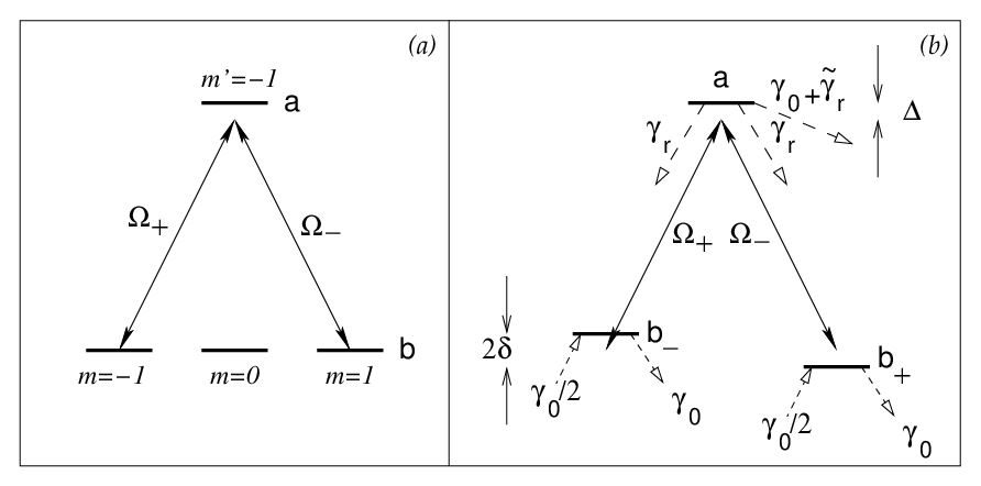
For zero magnetic field such a configuration demonstrates coherent population trapping. A nonzero magnetic field collinear with the wave vector of the light leads to Zeeman shift of magnetic sublevels $m=\pm 1$, which disturbs CPT and results in an interaction between the light and the atoms. The nonlinear polarization rotation emerges as a consequence of this interaction.

In the following, we briefly review the basic properties of CPT in $\Lambda$ systems and calculate the optical losses and the polarization rotation by solving the optical Bloch equations for the density matrix elements. Finally, we note how the $F=1\rightarrow F^{\prime}=0$ level configuration can be reduced to a $\Lambda$ system via proper renormalization of decay rates and density matrix.

II.1 Coherent population trapping in a $\Lambda$ system

The Hamiltonian for the $\Lambda$ system shown in Fig. 2b can be written as

$$H_{\Lambda} = \hbar\Delta|a\rangle\langle a|-\hbar\delta|b_{+}\rangle\langle b_{+}|+\hbar\delta|b_{-}\rangle\langle b_{-}|$$ (1)

$$+ \hbar\left(\Omega_{-}|a\rangle\langle b_{+}|+\Omega_{+}|a\rangle\langle b_{-}|+H.c.\ \right)$$

where $E_{+}$ and $E_{-}$ are the electric field amplitudes of two opposite circularly polarized electromagnetic waves, $\Omega_{-}=E_{-}\wp_{ab+}/\hbar$, $\Omega_{+}=E_{+}\wp_{ab-}/\hbar$ are the corresponding complex Rabi frequencies, $\wp_{ab+}$ and $\wp_{ab-}$ are the atomic dipole moments, $\Delta$ is the one-photon detuning of the laser frequency from the exact atomic transition, and $\delta$ is the shift of the ground-state sublevels resulting, for example, from interaction with a magnetic field.

The eigenvalues of this Hamiltonian $\lambda_{i}$ (where $H|\lambda\rangle=\hbar\lambda|\lambda\rangle$) may be found from

$$\left|\matrix{\delta-\lambda&\Omega_{+}^{*}&0\cr\Omega_{+}&\Delta-\lambda&\Omega_{-}\cr 0&\Omega_{-}^{*}&-\lambda-\delta}\right|=0$$ (2)

or

$$-\lambda^{3}+\lambda^{2}\Delta+\lambda(\delta^{2}+|\Omega_{+}|^{2}+|\Omega_{-}|^{2})-$$ (3)

$$\delta(\delta\Delta+|\Omega_{-}|^{2}-|\Omega_{+}|^{2})=0~.$$

In the degenerate case ($\delta=0$) the eigenvalues and corresponding eigenstates are

$$\lambda_{D} = 0$$

$$|D\rangle = \frac{\Omega_{+}|b_{+}\rangle-\Omega_{-}|b_{-}\rangle}{\sqrt{|\Omega_{+}|^{2}+|\Omega_{-}|^{2}}}$$ (4)

$$\lambda_{B_{1,2}} = \frac{\Delta}{2}\pm\sqrt{\frac{\Delta^{2}}{4}+|\Omega_{+}|^{2}+|\Omega_{-}|^{2}}$$

$$|B_{1,2}\rangle = \sqrt{\frac{|\lambda_{B_{1,2}}|}{\lambda_{B_{1}}-\lambda_{B_{2}}}}\left(|a\rangle+\frac{\Omega_{+}^{*}}{\lambda_{B_{1,2}}}|b_{-}\rangle+\frac{\Omega_{-}^{*}}{\lambda_{B_{1,2}}}|b_{+}\rangle\right)\,.$$

The state denoted as $|D\rangle$ is called the “dark state” because an atom in this state does not interact with the light fields and, therefore, does not fluoresce. Atoms in the other two states, called “bright states”, readily absorb light. Therefore, atoms initially prepared in a bright state are optically pumped into the dark state after some finite time comparable with the lifetime of the excited level $|a\rangle$. Thus, in steady-state, the atomic ensemble does not interact with the electro-magnetic fields, which is the essence of CPT. The dispersive properties of the atomic system in the dark state are governed by the coherence between the ground states of the $\Lambda$ system. The corresponding density matrix element may be found from (see Ref. 4):

$$\rho_{b+b-}=-\frac{\Omega_{-}^{*}\Omega_{+}}{|\Omega_{-}|^{2}+|\Omega_{+}|^{2}}~.$$ (6)

The true dark state exists only for $\delta=0$. As soon as the exact resonant conditions are disturbed, the system starts interacting with light. However, for small detunings ($\sqrt{|\Omega_{+}|^{2}+|\Omega_{-}|^{2}}\gg|\delta|,\ \sqrt{|\Delta\delta|}$) the disturbance of the dark state is small, and most of the atomic population is concentrated in the modified dark state $|\tilde{D}\rangle$. In this case the eigenvalue $\tilde{\lambda}_{D}$ corresponding to this state can be found by solving Eq. (3) and keeping only the terms linear in $\delta$:

$$\tilde{\lambda}_{D} = \delta\frac{|\Omega_{-}|^{2}-|\Omega_{+}|^{2}}{|\Omega_{+}|^{2}+|\Omega_{-}|^{2}}$$ (7)

$$|\tilde{D}\rangle \simeq \mathcal{N}\left\{|D\rangle+2\delta\frac{\Omega_{+}\Omega_{-}}{(|\Omega_{+}|^{2}+|\Omega_{-}|^{2})^{3/2}}|a\rangle\right\}$$ (8)

where $\mathcal{N}\simeq 1+O(\delta^{2})$ is a normalization constant. From Eq. (8) it is obvious that the population of the excited level $|a\rangle$ is proportional to $\delta^{2}$.

II.2 Equations of motion

It is possible to obtain the equation of motion for the electro-magnetic fields, using the method reported in Ref. [45, 46]. If we assume a small disturbance of CPT, almost all atomic population remains in a dark state during the interaction process, and we can rewrite the interaction Hamiltonian as

$$H\simeq\hbar\tilde{\lambda}_{D}|\tilde{D}\rangle\langle\tilde{D}|~.$$ (9)

Since now $|\tilde{D}\rangle\langle\tilde{D}|\simeq 1$, the atomic degrees of freedom may be excluded from the interaction picture and we can write $H\simeq\hbar\tilde{\lambda}_{D}$ . The interaction Hamiltonian may be rewritten in the Heisenberg picture, so that $\Omega\propto\hat{a}$, where $\hat{a}$ is the annihilation operator for the electromagnetic field [45]. The quantum mechanical equation for the electromagnetic creation and annihilation operators may be presented in the following form:

$$\frac{d\hat{a}}{dt}=-\frac{i}{\hbar}\frac{\partial H}{\partial\hat{a}^{\dagger}}~.$$ (10)

The propagation equation for the electromagnetic field amplitude $E$ can be obtained from Eq. (7) as a quasiclassical analogue of Eq. (10) [48]:

$$\frac{\partial E}{\partial z}=2\pi iN\frac{\nu}{c}\frac{\partial H}{\partial E^{*}}$$ (11)

where $N$ is the density of the atoms in the cell, and $\nu$ is a carrier frequency of the electromagnetic wave. Using Eqs. (11) and (7) (with $H\simeq\hbar\tilde{\lambda}_{D}$) we arrive at the following propagation equations for the Rabi frequencies $\Omega_{\pm}$:

$$\frac{\partial\Omega_{\pm}}{\partial z}=\mp 2i\kappa\delta\Omega_{\pm}\frac{|\Omega_{\mp}|^{2}}{(|\Omega_{+}|^{2}+|\Omega_{-}|^{2})^{2}}$$ (12)

where $\kappa$ is a coupling constant given by

$$\kappa=\frac{3}{8\pi}N\lambda^{2}\gamma_{r}$$ (13)

and $\lambda$ is the wavelength of the light in vacuum. It is also useful to rewrite the equation of motion for the field amplitudes $E_{\pm}$:

$$\frac{\partial E_{\pm}}{\partial z} = \mp 4i\pi\hbar\delta N\frac{\nu}{c}E_{\pm}\frac{|E_{\mp}|^{2}}{(|E_{+}|^{2}+|E_{-}|^{2})^{2}}~.$$ (14)

Equation (12) is suitable for describing the phase evolution of the electromagnetic fields. However the decay processes responsible for the optical losses cannot be correctly included in this method and we need a density matrix approach. In the following section we explicitly calculate the density matrix elements for the $\Lambda$ system to verify Eq. (12) and discuss the attenuation of the light.

II.3 Density matrix approach

In order to discuss a realistic model of the atom-field interaction in an atomic cell we need to include atomic level decay rates (Fig. 2b). We introduce the decay rate $\gamma_{0}$ outside of the system that is inversely proportional to the finite interaction time of the atoms and electromagnetic field. This decay represent the atoms leaving the interaction region. Another term that describes decay to outside levels, $\tilde{\gamma}_{r}$, describes population pumping into states that do not interact with the fields, for example, the state with zero magnetic moment ($m=0$ in Fig. 2a). The natural decay rate from level $|a\rangle$ to levels $|b_{+}\rangle$ or $|b_{-}\rangle$ is denoted as $\gamma_{r}$.

We also need to take into account the atoms entering the laser beam. To do that, we include incoherent pumping to all Zeeman sublevels from outside of the system, which means that atoms that enter the interaction region have equal populations of the ground state sublevels and no coherence between them. The value of the incoherent pumping rate is chosen to be $\gamma_{0}/2$ to keep the sum of level populations equal to unity in the case of $\tilde{\gamma}_{r}=0$. When $\tilde{\gamma}_{r}\neq 0$, the sum of the populations is less then unity because of the optical pumping, i.e.,

$$\rho_{aa}+\rho_{b+b+}+\rho_{b-b-}=1-\frac{\tilde{\gamma}_{r}}{\gamma_{0}}\rho_{aa}~.$$ (15)

The time-evolution equations for the density matrix elements $\rho_{ij}$ for the $\Lambda$ system can be obtained from the Liouville equation:

$$\dot{\rho}=-\frac{i}{\hbar}\left[H_{\Lambda},\rho\right]-\frac{1}{2}\{\Gamma,\rho\}+R$$ (16)

where $\rho=\sum\rho_{ij}|i\rangle\langle j|$, $H_{\Lambda}$ is given by Eq. (1), $\Gamma$ is the matrix describing the decays in the system, and $R$ is the matrix of incoherent pumping to the ground state sublevels. Then the equations for the atomic populations are:

$$\dot{\rho}_{b-\,b-} = \frac{\gamma_{0}}{2}-\gamma_{0}\rho_{b-\,b-}+\gamma_{r}\rho_{a\,a}$$ (17)

$$+i(\Omega_{+}^{*}\rho_{a\,b-}-c.c.)$$

$$\dot{\rho}_{b+\,b+} = \frac{\gamma_{0}}{2}-\gamma_{0}\rho_{b+\,b+}+\gamma_{r}\rho_{a\,a}$$ (18)

$$+i(\Omega_{-}^{*}\rho_{a\,b+}-c.c.)\,.$$

Analogously, for the polarizations we have

$$\dot{\rho}_{a\,b\pm} = -\Gamma_{a\,b\pm}\rho_{a\,b\pm}+i\Omega_{\mp}(\rho_{b\pm\,b\pm}-\rho_{a\,a})$$ (19)

$$+i\Omega_{\pm}\rho_{b\mp\,b\pm}$$

$$\dot{\rho}_{b-\,b+} = -\Gamma_{b-\,b+}\rho_{b-\,b+}+i\Omega_{+}^{*}\rho_{a\,b_{+}}$$ (20)

$$-i\Omega_{-}\rho_{b-\,a}$$

where

$$\Gamma_{a\,b\pm} = \gamma+i\left(\Delta\pm\delta\right)$$ (21)

$$\Gamma_{b-\,b+} = \gamma_{0}+2i\delta$$ (22)

with $\gamma=\gamma_{r}+\gamma_{0}+\tilde{\gamma}_{r}/2$.

In the steady state case, we can solve Eqs. (19) and (20) in terms of the atomic populations:

$$\rho_{b-\,b+} = -\frac{\Omega_{+}^{*}\Omega_{-}\left(\displaystyle\frac{n_{b-\,a}}{\Gamma_{b_{-}\,a}}+\displaystyle\frac{n_{b+\,a}}{\Gamma_{a\,b_{+}}}\right)}{\Gamma_{b-\,b+}+\displaystyle\frac{|\Omega_{+}|^{2}}{\Gamma_{a\,b+}}+\displaystyle\frac{|\Omega_{-}|^{2}}{\Gamma_{b-\,a}}}$$ (23)

$$\rho_{a\,b\pm} = \frac{i\Omega_{\mp}}{\Gamma_{a\,b\pm}}\displaystyle\frac{n_{b\pm\,a}\left(\Gamma_{b\mp\,b\pm}+\displaystyle\frac{|\Omega_{\mp}|^{2}}{\Gamma_{b\mp\,a}}\right)-n_{b\mp\,a}\displaystyle\frac{|\Omega_{\pm}|^{2}}{\Gamma_{b\mp\,a}}}{\Gamma_{b\mp\,b\pm}+\displaystyle\frac{|\Omega_{\pm}|^{2}}{\Gamma_{a\,b\pm}}+\displaystyle\frac{|\Omega_{\mp}|^{2}}{\Gamma_{b\mp\,a}}}$$

where $n_{b\pm\,a}\equiv\rho_{b\pm\,b\pm}-\rho_{aa}$ . Inserting these expressions into Eqs. (17) and (18) and using the condition given in Eq. (15) we can derive linear equations for the atomic populations. In the general case, however, their solution is very cumbersome.

Let us consider the case of a strong electro-magnetic field, such that $|\Omega|^{2}/\gamma_{0}\gamma\gg 1$. We also assume that $|\delta|,\gamma_{0}\ll\gamma,|\Omega|$, and $\Delta=0$. In the zeroth approximation the atomic populations are determined by Eq. (7):

$$\rho_{b\pm\,b\pm}^{(0)} \simeq \frac{|\Omega_{\pm}|^{2}}{|\Omega|^{2}}$$ (25)

$$\rho_{a\,a}^{(0)} \simeq 0$$ (26)

where $|\Omega|^{2}=|\Omega_{+}|^{2}+|\Omega_{-}|^{2}$.

Now we can solve for the polarizations $\rho_{a\,b\pm}$ , keeping only the terms linear in $\delta$ and $\gamma_{0}$

$$\rho_{a\,b\pm}\simeq\frac{i\Omega_{\mp}}{|\Omega|^{4}}\left(\frac{\gamma_{0}}{2}|\Omega|^{2}\pm 2i\delta|\Omega_{\pm}|^{2}\right)~.$$ (27)

It is important to note that this expression for the polarization, obtained for an open $\Lambda$ system, coincides with the analogous expression calculated by Fleischhauer et al. [5] for a closed system, if the ground-state coherence decay rate and the population exchange rate between ground states are the same and equal to $\gamma_{0}$. This proves the equivalence of the open and closed models for the description of $\Lambda$ schemes, which has been previously demonstrated by Lee et al. [49] for the particular case of a weak probe field.

The stationary propagation of two circularly polarized components of the laser field through the atomic medium is described by Maxwell-Bloch equations for the slowly-varying amplitudes and phases:

$$\frac{\partial\Omega_{\pm}}{\partial z}\simeq-\kappa\frac{\Omega_{\pm}}{|\Omega|^{4}}\left(\frac{\gamma_{0}}{2}|\Omega|^{2}\pm 2i\delta|\Omega_{\mp}|^{2}\right).$$ (28)

Note that Eq. (12) can be obtained from Eq. (28) in the limit $\gamma_{0}=0$.

Separating the real and imaginary parts of Eq. (28) and using $\Omega_{\pm}=|\Omega_{\pm}|~e^{i\phi_{\pm}}$ , one can find the propagation equations of the electromagnetic field intensity $|\Omega|^{2}$ and the rotation angle of the polarization ellipse $\phi=(\phi_{+}-\phi_{-})/2$:

$$\frac{\partial|\Omega|^{2}}{\partial z} = -\kappa\gamma_{0}$$ (29)

$$\frac{\partial\phi}{\partial z} = -\frac{2\kappa\delta}{|\Omega|^{2}}.$$ (30)

After integration, the following expressions for the light transmission $I_{\mathrm{out}}$ and the polarization rotation angle $\phi$ are obtained:

$$I_{\mathrm{out}} = I_{in}\left(1-\frac{\kappa\gamma_{0}L}{|\Omega(0)|^{2}}\right)$$ (31)

$$\phi = \frac{2\delta}{\gamma_{0}}\ln\frac{I_{in}}{I_{out}}$$ (32)

where $L$ is the interaction length. It is important to note that the final expressions in Eqs. (31) and (32) include only the total laser intensity, not the intensities of the individual circular components. This means that both transmission and polarization rotation are independent of the initial polarization of light [50].

II.4 Normalization conditions for an $F=1\rightarrow F^{\prime}=0$ transition

The correspondence between the $F=1\rightarrow F^{\prime}=0$ scheme (Figs. 2a) and $\Lambda$ scheme (Fig. 2b) can be obtained if we exchange $\gamma_{r}$ by $\gamma_{aa}/3$, where $\gamma_{aa}$ is the decay rate of the excited state to the ground state. The decay rate $\tilde{\gamma}_{r}$ should be presented as $\tilde{\gamma}_{r}=\gamma_{aa}/3+\tilde{\gamma}_{aa}$, where $\tilde{\gamma}_{aa}$ stands for the decay of the excited state outside of the system in Fig. 2a.

We assume that the incoherent pumping rate into each Zeeman ground state is equal to $\gamma_{0}/3$, to keep the normalization condition similar to Eq. (15):

$$\tilde{\rho}_{aa}+\rho_{+1,+1}+\rho_{-1,-1}+\rho_{0,0}=1-\frac{\tilde{\gamma}_{aa}}{\gamma_{0}}\tilde{\rho}_{aa}$$ (33)

where $\tilde{\rho}_{aa}$ is the population of the excited state and $\rho_{ii}$ is the population of the $i$th magnetic sublevel of the ground state in the system depicted in Fig. 2a.

Keeping in mind that the population of the $m=0$ state is determined by the decay rate of excited state $|a\rangle$ and by the decay outside of the system we write the rate equation

$$\dot{\rho}_{0,0}=\frac{\gamma_{0}}{3}-\gamma_{0}\rho_{0,0}+\frac{\gamma_{aa}}{3}\tilde{\rho}_{aa}$$ (34)

and solve it in the steady state

$$\rho_{0,0}=\frac{1}{3}+\frac{\gamma_{aa}}{3\gamma_{0}}\tilde{\rho}_{aa}~.$$ (35)

Let us assume that $\tilde{\rho}_{aa}=\xi\rho_{aa}$, $\rho_{+1,+1}=\xi\rho_{b+b+}$, and $\rho_{-1,-1}=\xi\rho_{b-b-}$. The normalization parameter $\xi$ can be found by substituting Eq. (35) into Eq. (33), and comparing the normalization conditions Eqs. (15) and (33):

$$\xi=\frac{2}{3}.$$ (36)

Therefore, we can derive density matrix elements for the $F=1\rightarrow F^{\prime}=0$ level scheme shown in Fig. 2a by simple multiplication of the elements of the density matrix for the $\Lambda$ scheme by the scaling factor $\xi$.

III Analysis of NMOR for the case of an $F=2\rightarrow F^{\prime}=1$ transition

For atomic ground atomic state angular momentum higher than $F=1$ it is possible to create more than one $\Lambda$ link between magnetic sublevels. This is equivalent to the creation of coherent atomic states characterized by higher angular momenta, which may drastically change the interaction of such a medium with the electromagnetic field.

Let us concentrate first on $F=2\rightarrow F^{\prime}=1$ transitions, which occur in the ⁸⁷Rb $\mathrm{D}_{1}$ line. The case of higher angular momenta is discussed in the next section. Interaction of elliptically polarized light with the $F=2\rightarrow F^{\prime}=1$ transition may be decomposed into a $\Lambda$ scheme with $m=-1\leftrightarrow m^{\prime}=0\leftrightarrow m=+1$, and an $M$ scheme $m=-2\leftrightarrow m^{\prime}=-1\leftrightarrow m=0\leftrightarrow m^{\prime}=+1\leftrightarrow m=+2$, as shown in Fig. 3a. The main difference of between an $M$ scheme and a $\Lambda$ scheme is that the higher order coherence ($\Delta m=4$) becomes important. Since the $\Lambda$ system had been studied in the previous section, we primarily concentrate on $M$ scheme here.

Figure 3: a) Energy level scheme for ⁸⁷Rb atoms. This scheme may be decomposed into a superposition of b) $\Lambda$-system and c) $M$-system. Transition probabilities are shown for each individual transition.

The $M$ scheme is described by a set of twelve density matrix equations. The only straightforward way to solve this system is with numerical methods. However, if we study the atomic interactions with weak magnetic fields, the decay processes and polarization rotation processes are independent, as we saw for the $\Lambda$ configuration. Thus, the polarization rotation may be found in analytical form under the condition of zero relaxation using the Hamiltonian diagonalization procedure as presented for the $\Lambda$ system. The modified Schrödinger equation model is suited for this as well. The optical losses may be found separately by considering the optical pumping into the dark state with zero magnetic field.

III.1 Coherent population trapping in an $M$ level scheme

It has been shown that the dark state exists even for atoms with complicated Zeeman substructure interacting with elliptically polarized light [51, 52, 53, 54, 55, 56]. Here we recall the analytical expressions for this dark state and the corresponding eigenvalues. Using an effective interaction Hamiltonian, we derive propagation equations for the electromagnetic fields. We restrict our consideration to the case relevant to the $M$ configuration consisting of Zeeman energy sublevels in the magnetic field. That is, we assume that the atomic transition frequencies are such that $\omega_{a-b0}=\omega_{a+b0}=\omega$, $\omega_{a-b-}=\omega-2\delta$, and $\omega_{a+b+}=\omega+2\delta$, where the detuning $\delta$ is due to a Zeeman shift, and the laser frequency $\nu$ is resonant with the atomic transition. The interaction Hamiltonians for $M$ systems is

$$H_{M} = -2\hbar\delta|b_{+}\rangle\langle b_{+}|+2\hbar\delta|b_{-}\rangle\langle b_{-}|$$ (37)

$$+ \hbar(\Omega_{1-}|a_{+}\rangle\langle b_{+}|+\Omega_{2-}|a_{-}\rangle\langle b_{0}|$$

$$+ \Omega_{1+}|a_{+}\rangle\langle b_{0}|+\Omega_{2+}|a_{-}\rangle\langle b_{-}|+H.c.),$$

where $\Omega_{1-}=E_{-}\wp_{a+b+}/\hbar$, $\Omega_{1+}=E_{+}\wp_{a+b0}/\hbar$, $\Omega_{2-}=E_{-}\wp_{a-b0}/\hbar$, $\Omega_{2+}=E_{+}\wp_{a-b-}/\hbar$ (see Fig. 3c).

As in the $\Lambda$ system, the eigenvalues of the interaction Hamiltonian can be determined from:

$$\left|\matrix{2\delta-\lambda&\Omega_{2+}^{*}&0&0&0\cr\Omega_{2+}&-\lambda&\Omega_{2-}&0&0\cr 0&\Omega_{2-}^{*}&-\lambda&\Omega_{1+}^{*}&0\cr 0&0&\Omega_{1+}&-\lambda&\Omega_{1-}\cr 0&0&0&\Omega_{1-}^{*}&-\lambda-2\delta}\right|=0$$ (38)

Also, as in the $\Lambda$ scheme, the eigenvalue $\lambda=0$ and corresponding “dark state” exists only for $\delta=0$:

$$|D\rangle=\frac{\Omega_{1+}\Omega_{2+}|b_{+}\rangle-\Omega_{1-}\Omega_{2+}|b_{0}\rangle+\Omega_{1-}\Omega_{2-}|b_{-}\rangle}{\sqrt{|\Omega_{1-}|^{2}|\Omega_{2+}|^{2}+|\Omega_{1+}|^{2}|\Omega_{2+}|^{2}+|\Omega_{1-}|^{2}|\Omega_{2-}|^{2}}}$$ (39)

It is worth noting that, similar to the $\Lambda$ system, the non-vanishing low frequency coherences $\rho_{b+b0}$ and $\rho_{b0b-}$ are important here. The major difference in the dispersive properties of the $M$ and $\Lambda$ schemes arises from the existence of the four-photon coherence $\rho_{b+b-}$:

$$\rho_{b+b-}=\frac{\Omega_{1-}^{*}\Omega_{2-}^{*}\Omega_{1+}\Omega_{2+}}{|\Omega_{1-}|^{2}|\Omega_{2+}|^{2}+|\Omega_{1+}|^{2}|\Omega_{2+}|^{2}+|\Omega_{1-}|^{2}|\Omega_{2-}|^{2}}~.$$ (40)

For small $\delta$ we can again find the eigenvalue for the quasi-dark state, taking into account only the linear terms in $\delta$:

$$\tilde{\lambda}_{M}=2\delta\frac{|\Omega_{2-}|^{2}|\Omega_{1-}|^{2}-|\Omega_{2+}|^{2}|\Omega_{1+}|^{2}}{|\Omega_{2+}|^{2}|\Omega_{1+}|^{2}+|\Omega_{2-}|^{2}|\Omega_{1-}|^{2}+|\Omega_{2+}|^{2}|\Omega_{1-}|^{2}}~.$$ (41)

Using Eq. (11) we derive equations of motion for the fields. For example,

$$\frac{\partial\Omega_{2-}}{\partial z}=2i\kappa\delta\Omega_{2-}\frac{\wp_{a-b0}^{2}}{\wp^{2}}$$ (42)

$$\frac{2|\Omega_{1+}|^{2}|\Omega_{1-}|^{2}|\Omega_{2+}|^{2}+|\Omega_{2+}|^{2}|\Omega_{1-}|^{4}}{(|\Omega_{1-}|^{2}|\Omega_{2+}|^{2}+|\Omega_{1+}|^{2}|\Omega_{2+}|^{2}+|\Omega_{1-}|^{2}|\Omega_{2-}|^{2})^{2}}$$

where $\kappa$ is the coupling constant with respect to the transition as a whole (i.e., $\gamma_{r}$ in Eq. (13) is now the total natural decay rate of the excited state), and $\wp=(4\nu^{3}\gamma_{r}/(3\hbar c^{3}))^{1/2}$ is the dipole moment of the transition.

The calculations can be considerably simplified if the numerical values of the transition probabilities are used. Let us now consider the particular case of the $M$ part of the $F=2\rightarrow F=1$ transition. According to the transition probabilities, shown in Fig. 3c, we get $|\Omega_{2+}|^{2}/|\Omega_{2-}|^{2}=6|E_{+}|^{2}/|E_{-}|^{2}$ and $|\Omega_{1+}|^{2}/|\Omega_{1-}|^{2}=|E_{+}|^{2}/6|E_{-}|^{2}$. The interaction Hamiltonian ($H_{M}\simeq\hbar\tilde{\lambda}_{M}$) for the elliptically polarized laser field can therefore be rewritten as

$$H_{M}\simeq 2\hbar\delta\frac{|E_{-}|^{4}-|E_{+}|^{4}}{|E_{+}|^{4}+|E_{-}|^{4}+6|E_{+}|^{2}|E_{-}|^{2}}$$ (43)

and therefore

$$\frac{\partial E_{\pm}}{\partial z} = \mp 8i\pi\hbar\delta N\frac{\nu}{c}E_{\pm}\times$$ (44)

$$|E_{\mp}|^{2}\frac{3(|E_{+}|^{4}+|E_{-}|^{4})+2|E_{+}|^{2}|E_{-}|^{2}}{(|E_{+}|^{4}+|E_{-}|^{4}+6|E_{+}|^{2}|E_{-}|^{2})^{2}}\,.$$

In what follows we derive the same equation using the more rigorous modified Schrödinger formalism [57].

III.2 Solution based on the modified Schrödinger equations

The interaction described above of the four electromagnetic fields with the $M$ energy level configuration may be also studied using Schrödinger equations. This approach enables us to find exact expressions for all the atomic observables when we can ignore spontaneous emission. The state vector of the atom can be written as:

$$|\Psi\rangle = a_{+}e^{-i\nu t}|a_{+}\rangle+a_{-}e^{-i\nu t}|a_{-}\rangle+$$ (45)

$$b_{0}|b_{0}\rangle+b_{+}|b_{+}\rangle+b_{-}|b_{-}\rangle\,.$$

Solving the Schrödinger equation

$$|\dot{\Psi}\rangle=-\frac{i}{\hbar}\hat{H}|\Psi\rangle$$

for the interaction Hamiltonian Eq. (37), we obtain the following equations of motion for the slowly-varying state amplitudes:

$$\dot{a}_{+} = i\Omega_{1+}b_{0}+i\Omega_{1-}b_{+}$$ (46)

$$\dot{a}_{-} = i\Omega_{2+}b_{-}+i\Omega_{2-}b_{0}$$ (47)

$$\dot{b}_{+} = 2i\delta b_{+}+i\Omega_{1-}^{*}a_{+}$$ (48)

$$\dot{b}_{-} = -2i\delta b_{-}+i\Omega_{2+}^{*}a_{-}$$ (49)

$$\dot{b}_{0} = i\Omega_{1+}^{*}a_{+}+i\Omega_{2-}^{*}a_{-}~.$$ (50)

In the steady state regime, this system has a nontrivial solution only for $\delta=0$. The solutions for nonzero detunings correspond to zero amplitudes for all parameters. Thus, to sustain steady state in the open system, external pumping is necessary. For a small splitting between ground state levels $\hbar\delta\ll kT$, where $T$ is the temperature of the vapor, we assume that in thermal equilibrium, i.e., in the absence of all fields, all lower states $|b_{\pm}\rangle$ and $|b_{0}\rangle$ are equally populated. And, therefore, within the open-system approach, we assume that the atoms are pumped into states $|b_{+}\rangle$, $|b_{-}\rangle$, or $|b_{0}\rangle$ with equal probability from outside of the system. The corresponding rate can be determined by the requirement that the total probability to find an atom in any of the states is unity.

Unlike the density matrix approach, a straightforward introduction of incoherent pumping into the ground states of the system is impossible. It was shown by Fleischhauer [57] in an elegant way that the effective density matrix equations for open systems with injection rates into states and decays out of states can be written in terms of stochastic complex state amplitudes.

Let us consider an effective density matrix equation for an atomic ensemble undergoing a unitary interaction with some external fields or potentials. In addition, decay out of atomic states $|j\rangle$ is taken into account with rates $\gamma_{j}$. Also injection into certain states is considered with injection rates $R_{ij}$. In our case the injection occurs only into energy eigenstates of the atoms or incoherent mixtures of them, so only diagonal elements of the matrix $R_{ij}$ are nonzero. If injection in the coherent superposition states is considered, non-diagonal elements are also required to be taken into account.

An effective density matrix equation has the following structure:

$${\dot{\rho}}_{ij}(t)=R_{ij}-\frac{\gamma_{i}+\gamma_{j}}{2}\rho_{jj}-\frac{i}{\hbar}\Bigl[H,\rho\Bigr]_{ij}$$ (51)

where $\gamma_{i}$ are decay rates out of the system, which can in general be different for individual states. Generally, the pump rates $R_{ij}$ are time dependent, but for the sake of simplicity we assume in the following that the rates $R_{ij}$ are constant.

Density matrix elements may be represented in terms of state amplitudes $\rho_{ji}=c_{i}^{*}c_{j}$ . In order to put the pump term $R_{ij}$ in a similar form, we introduce a formal Gaussian stochastic variable $r_{i}$ with the following properties:

$$\langle r_{i}\rangle = 0$$ (52)

$$\langle r_{i}r_{j}\rangle = 0$$ (53)

$$\langle r_{i}^{*}r_{j}\rangle = R_{ij}~.$$ (54)

This yields a set of amplitude equations with stochastic pump terms:

$${\dot{c}}_{i}=r_{i}-\frac{\gamma_{i}}{2}\,c_{i}+\frac{i}{\hbar}H_{ij}\,c_{j}~.$$ (55)

Since the amplitude equations are linear, their solution will be a linear functional of the stochastic pump rates $r_{i}$. Thus the averaging of bilinear quantities such as $c_{i}^{*}c_{j}$ required to obtain the density matrix elements can easily be performed. Generally, solution $c_{j}$ of Eq. (55) no longer makes sense as the amplitude for the atomic wave function. It only determines density matrix elements of the system.

To apply the above technique to our problem, we rewrite Eqs. (46)–(50) (with time derivatives set equal to zero)

$$i\Omega_{1+}b_{0}+i\Omega_{1-}b_{+}=0$$ (56)

$$i\Omega_{2+}b_{-}+i\Omega_{2-}b_{0}=0$$ (57)

$$2i\delta b_{+}+i\Omega_{1-}^{*}a_{+}=ir_{+}$$ (58)

$$-2i\delta b_{-}+i\Omega_{2+}^{*}a_{-}=ir_{-}$$ (59)

$$i\Omega_{1+}^{*}a_{+}+i\Omega_{2-}^{*}a_{-}=ir_{0}$$ (60)

where the stochastic “pumping” is introduced

$$\langle r_{\pm}\rangle = \langle r_{0}\rangle=0$$

$$\langle r_{\pm}r_{\mp}\rangle = \langle r_{\pm}r_{0}\rangle=0$$

$$\langle r_{\pm}^{*}r_{\mp}\rangle = \langle r_{\pm}^{*}r_{0}\rangle=0$$

$$\langle r_{\pm}^{*}r_{\pm}\rangle = \langle r_{0}^{*}r_{0}\rangle=r^{2}~.$$

Solving Eqs. (56)–(60) with respect to $a_{1}$, $a_{2}$, $b_{\pm}$, and $b_{0}$ we get

$$b_{+} = -b_{0}\frac{\Omega_{1+}}{\Omega_{1-}}~,\;\;\;b_{-}=-b_{0}\frac{\Omega_{2-}}{\Omega_{2+}}$$

$$b_{0} = \frac{r_{+}|\Omega_{2+}|^{2}\Omega_{1-}\Omega_{1+}^{*}+r_{-}|\Omega_{1-}|^{2}\Omega_{2+}\Omega_{2-}^{*}-r_{0}|\Omega_{1-}|^{2}|\Omega_{2+}|^{2}}{2\delta\left(|\Omega_{1+}|^{2}|\Omega_{2+}|^{2}-|\Omega_{1-}|^{2}|\Omega_{2-}|^{2}\right)}$$

$$a_{-} = \frac{r_{+}\Omega_{1+}^{*}\Omega_{1-}\Omega_{2-}+r_{-}|\Omega_{1+}|^{2}\Omega_{2+}-r_{0}|\Omega_{1-}|^{2}\Omega_{2-}}{|\Omega_{1+}|^{2}|\Omega_{2+}|^{2}-|\Omega_{1-}|^{2}|\Omega_{2-}|^{2}}$$

$$a_{+} = -\frac{r_{+}|\Omega_{2-}|^{2}\Omega_{1-}+r_{-}\Omega_{2-}^{*}\Omega_{1+}\Omega_{2+}-r_{0}|\Omega_{2+}|^{2}\Omega_{1+}}{|\Omega_{1+}|^{2}|\Omega_{2+}|^{2}-|\Omega_{1-}|^{2}|\Omega_{2-}|^{2}}~.$$ (61)

Utilizing the normalization condition

$$\langle a_{-}^{*}a_{-}\rangle+\langle a_{+}^{*}a_{+}\rangle+\langle b_{+}^{*}b_{+}\rangle+\langle b_{-}^{*}b_{-}\rangle+\langle b_{0}^{*}b_{0}\rangle=1$$ (62)

we get

$$r=2\delta\left(|\Omega_{1+}|^{2}|\Omega_{2+}|^{2}-|\Omega_{1-}|^{2}|\Omega_{2-}|^{2}\right)/$$ (63)

$$\left\{(|\Omega_{1-}|^{2}|\Omega_{2+}|^{2}+|\Omega_{1+}|^{2}|\Omega_{2+}|^{2}+|\Omega_{1-}|^{2}|\Omega_{2-}|^{2})^{2}+\right.$$

$$\left.4\delta^{2}\left[|\Omega_{1+}|^{2}|\Omega_{1-}|^{2}(|\Omega_{1+}|^{2}+|\Omega_{2+}|^{2})+\right.\right.$$

$$\left.\left.2(|\Omega_{1+}|^{4}|\Omega_{2+}|^{2}+|\Omega_{1-}|^{4}|\Omega_{2-}|^{2})\right]\right\}^{1/2}~.$$

Using Eq. (63) we arrive at the complete solution of the problem which takes into account all orders in $\delta$. For $\delta=0$ the system is in a dark state and the density matrix elements correspond to the elements generated by Eq. (39). For a nonzero small two-photon detuning the populations and coherences for the ground state stay approximately unchanged. The solution for the populations of the excited states are

$$\rho_{a-a-}=4\delta^{2}\frac{|\Omega_{1+}|^{2}|\Omega_{1-}|^{2}|\Omega_{2-}|^{2}+|\Omega_{1+}|^{4}|\Omega_{2+}|^{2}+|\Omega_{1-}|^{4}|\Omega_{2-}|^{2}}{(|\Omega_{1-}|^{2}|\Omega_{2+}|^{2}+|\Omega_{1+}|^{2}|\Omega_{2+}|^{2}+|\Omega_{1-}|^{2}|\Omega_{2-}|^{2})^{2}}$$ (64)

$$\rho_{a+a+}=4\delta^{2}\frac{|\Omega_{2+}|^{2}|\Omega_{2-}|^{2}|\Omega_{1+}|^{2}+|\Omega_{2+}|^{4}|\Omega_{1+}|^{2}+|\Omega_{2-}|^{4}|\Omega_{1-}|^{2}}{(|\Omega_{1-}|^{2}|\Omega_{2+}|^{2}+|\Omega_{1+}|^{2}|\Omega_{2+}|^{2}+|\Omega_{1-}|^{2}|\Omega_{2-}|^{2})^{2}}$$ (65)

and for the atomic polarizations are

$$\rho_{a-b0}=\frac{2\delta\Omega_{2-}(2|\Omega_{1+}|^{2}|\Omega_{1-}|^{2}|\Omega_{2+}|^{2}+|\Omega_{2+}|^{2}|\Omega_{1-}|^{4})}{(|\Omega_{1-}|^{2}|\Omega_{2+}|^{2}+|\Omega_{1+}|^{2}|\Omega_{2+}|^{2}+|\Omega_{1-}|^{2}|\Omega_{2-}|^{2})^{2}}$$ (66)

$$\rho_{a+b0}=-\frac{2\delta\Omega_{1+}(2|\Omega_{1-}|^{2}|\Omega_{2+}|^{2}|\Omega_{2-}|^{2}+|\Omega_{1-}|^{2}|\Omega_{2+}|^{4})}{(|\Omega_{1-}|^{2}|\Omega_{2+}|^{2}+|\Omega_{1+}|^{2}|\Omega_{2+}|^{2}+|\Omega_{1-}|^{2}|\Omega_{2-}|^{2})^{2}}$$ (67)

$$\rho_{a-b-}=-\frac{2\delta\Omega_{2+}(2|\Omega_{1+}|^{2}|\Omega_{1-}|^{2}|\Omega_{2-}|^{2}+|\Omega_{2-}|^{2}|\Omega_{1-}|^{4})}{(|\Omega_{1-}|^{2}|\Omega_{2+}|^{2}+|\Omega_{1+}|^{2}|\Omega_{2+}|^{2}+|\Omega_{1-}|^{2}|\Omega_{2-}|^{2})^{2}}$$ (68)

$$\rho_{a+b+}=\frac{2\delta\Omega_{1-}(2|\Omega_{1+}|^{2}|\Omega_{2+}|^{2}|\Omega_{2-}|^{2}+|\Omega_{1+}|^{2}|\Omega_{2+}|^{4})}{(|\Omega_{1-}|^{2}|\Omega_{2+}|^{2}+|\Omega_{1+}|^{2}|\Omega_{2+}|^{2}+|\Omega_{1-}|^{2}|\Omega_{2-}|^{2})^{2}}~.$$ (69)

Here we kept only the lowest order terms in $\delta$. In the expressions for the atomic polarizations, the first term, containing the amplitude of all four optical fields (for example, $\Omega_{1+}|\Omega_{1-}|^{2}|\Omega_{2+}|^{2}|\Omega_{2-}|^{2}$ in the equation for $\rho_{a+b0}$), is due to the four-photon coherence (hexadecapole moment), whereas the second term represents the effect of optical pumping.

The propagation equation for the fields is

$$\frac{\partial\Omega_{ij}}{\partial z} = i\frac{2\pi\nu}{c}N\frac{\wp_{ij}^{2}}{\hbar}\rho_{ij}$$ (70)

where the indexes $ij$ show that the values are related to the same transition $|i\rangle\rightarrow|j\rangle$. It is easy to see, for example, that the matrix element in Eq. (66) results in the propagation equation in Eq. (42). The two approaches are therefore equivalent. The equation of motion for the circularly polarized electromagnetic fields in $E_{\pm}$ are given by the following expressions:

$$\frac{\partial E_{+}}{\partial z} = i\frac{2\pi\nu}{c}N\left(\wp_{a-b-}\rho_{a-b-}+\wp_{a+b0}\rho_{a+b0}\right)$$ (71)

$$\frac{\partial E_{-}}{\partial z} = i\frac{2\pi\nu}{c}N\left(\wp_{a+b+}\rho_{a+b+}+\wp_{a-b0}\rho_{a-b0}\right)\,.$$ (72)

Substituting the expressions for atomic polarizations Eqs. (66)–(69) and using the proper dipole moments for each transition (for the ⁸⁷Rb they are equal $1/2$ for $|b_{\pm}\rangle\rightarrow|a_{\pm}\rangle$, and $1/12$ for $|b_{0}\rangle\rightarrow|a_{\pm}\rangle$ (Fig. 3c)), we obtain Eqs. (44).

So far we have made no assumption concerning the losses in the system. Generally, this requires solving the Bloch equations for the atomic populations and polarizations as was done for the $\Lambda$ system. For the $M$ scheme, however, this process is rather involved even for the degenerate system ($\delta=0$). Since the dark state exists for any value of Rabi frequency $\Omega_{ij}$, it is always possible to transform the basis of the atomic states so that there is one atomic level uncoupled from the laser field. The $M$ system can be represented as two independent open two-level systems, connected only via relaxation processes [58]. The absorption in this systems has similar properties compared to those of the $\Lambda$ system: it is proportional to decay rate $\gamma_{0}$ and inversely proportional to the light intensity. The exact analytical expression for this absorption is rather lengthy and we do not present it here.

III.3 Polarization rotation for an $F=2\rightarrow F^{\prime}=1$ transition

To describe the polarization rotation on the $F=2\rightarrow F^{\prime}=1$ transition we write the interaction Hamiltonian as a balanced sum of the Hamiltonians for the $M$ and $\Lambda$ systems, taking into account the branching ratio for the atomic transitions

$$H_{2\rightarrow 1}=\zeta_{1}H_{\Lambda}+\zeta_{2}H_{M}=\zeta_{1}\hbar\tilde{\lambda}_{\Lambda}+\zeta_{2}\hbar\tilde{\lambda}_{M}$$ (73)

where $\zeta_{1}$ and $\zeta_{2}$ are weighting coefficients ($\zeta_{1}+\zeta_{2}=1$) that describe the population redistribution between the $\Lambda$ and $M$ schemes. Using the numerical simulation of this system, we find them to be equal with very good accuracy. Using Eq. (11) we now derive the equation of motion for this system:

$$\frac{\partial E_{\pm}}{\partial z}=\mp 4i\pi\hbar\delta N\frac{\nu}{c}E_{\pm}\frac{|E_{\mp}|^{2}}{(|E_{+}|^{2}+|E_{-}|^{2})^{2}}\left[1+2(|E_{+}|^{2}+|E_{-}|^{2})^{2}\frac{3(|E_{+}|^{4}+|E_{-}|^{4})+2|E_{+}|^{2}|E_{-}|^{2}}{(|E_{+}|^{4}+|E_{-}|^{4}+6|E_{+}|^{2}|E_{-}|^{2})^{2}}\right].$$ (74)

It is interesting to note that for linearly polarized light ($|\Omega_{+}|=|\Omega_{-}|$) the contributions from $\Lambda$ and $M$ system are identical, and Eq. (74) coincides with Eq. (14). This proves that a single $\Lambda$ system may be used for accurate description of the dispersive properties of more complicated level configurations.

Let us introduce the electromagnetic field ellipticity parameter $q$ such that the amplitudes of the circularly polarized components are $E_{\pm}=|E|\sqrt{(1\pm q)}\exp(i\phi_{\pm})/\sqrt{2}$. Then Eq. (74) transforms to

$$\frac{\partial E_{\pm}}{\partial z}=\mp 2i\pi\hbar\delta N\frac{\nu}{c}\frac{E_{\pm}(1\mp q)}{|E|^{2}}\left[1+2\frac{2+q^{2}}{(2-q)^{2}}\right]~.$$ (75)

Based of the results of our numerical simulation, we conclude that absorption of light that interacts with the $F=2\rightarrow F^{\prime}=1$ transition does not depend on the ellipticity of the light. The light transmission through the cell can be described by an equation similar to Eq. (31):

$$I_{\mathrm{\mathrm{out}}} = I_{\mathrm{in}}\left(1-\frac{2\pi\hbar\gamma_{0}NL}{|E(0)|^{2}}\frac{\nu}{c}\right).$$ (76)

The rotation angle for the light polarization is then given by

$$\phi = \frac{\delta}{\gamma_{0}}\left[1+2\frac{2+q^{2}}{(2-q^{2})^{2}}\right]{\rm ln}\frac{I_{\mathrm{in}}}{I_{\mathrm{out}}}$$ (77)

where $I_{\mathrm{in}}$ and $I_{\mathrm{out}}$ are the intensities of the electromagnetic field at the entrance and exit of the medium. The value of polarization rotation increases with the light ellipticity by the factor

$$\frac{\phi_{M+\Lambda}}{\phi_{\Lambda}}=\frac{1}{2}\left(1+2\frac{2+q^{2}}{(2-q^{2})^{2}}\right)$$ (78)

compared to $\Lambda$ system. Therefore NMOR on the $F=2\rightarrow F^{\prime}=1$ transition may only be properly described by a $\Lambda$ configuration for linearly polarized light. The difference between the $M$ and $\Lambda$ systems results from the hexadecapole moment induced in $M$ configuration.

IV NMOR in atoms with large values of angular momentum

Higher order coherence can be excited among Zeeman sublevels of alkali atoms with $F>2$. Here we find a perturbed dark state for the generalized $M$ scheme consisting of an arbitrary number of $\Lambda$-links, using the method described above. Then we apply these results to evaluate the nonlinear Faraday rotation in the ⁸⁵Rb $F=3\rightarrow F=2$ transition. We consider the scheme in Fig. 5. The interaction Hamiltonian for this scheme is

$$H_{n\times\Lambda} = -\hbar\delta\sum_{k=0}^{n}(n-2k)|b_{k+1}\rangle\langle b_{k+1}|$$ (79)

$$+ \hbar\sum_{k=1}^{n}\left(\Omega_{k-}|a_{k}\rangle\langle b_{k}|+\Omega_{k+}|a_{k}\rangle\langle b_{k+1}|+H.c.\right)$$

Here $n$ is the number of $\Lambda$ links, which connects $n+1$ ground-state levels via $n$ excited states. There exists a dark state for this system for exact resonance ($\delta$=0):

$$|D\rangle=\frac{\displaystyle\sum\limits_{k=0}^{n}(-1)^{k}\displaystyle\prod_{j=1}^{k}\Omega_{j-}\displaystyle\prod\limits_{l=k+1}^{n}\Omega_{l+}\ |b_{k+1}\rangle}{\sqrt{\displaystyle\sum\limits_{k=0}^{n}\displaystyle\prod_{j=1}^{k}|\Omega_{j-}|^{2}\displaystyle\prod\limits_{l=k+1}^{n}|\Omega_{l+}|^{2}}}$$ (80)

where we use a convention that $\prod_{j=1}^{0}\equiv\prod_{j=n+1}^{n}\equiv 1$. We deduce the perturbed “dark state” eigenvalue for the Hamiltonian using the same procedure as we used before in Eq. (79)

$$\tilde{\lambda}_{n\times\Lambda}\simeq\delta\frac{\displaystyle\sum\limits_{k=0}^{n}(2k-n)\displaystyle\prod\limits_{i=1}^{k}|\Omega_{i-}|^{2}\displaystyle\prod\limits_{j=k+1}^{n}|\Omega_{j+}|^{2}}{\displaystyle\sum\limits_{k=0}^{n}\displaystyle\prod\limits_{i=1}^{k}|\Omega_{i-}|^{2}\displaystyle\prod\limits_{j=k+1}^{n}|\Omega_{j+}|^{2}}~.$$ (81)

The equation of motion for the circularly polarized electromagnetic fields can be found from Eq. (11). As an example, let us calculate the interaction Hamiltonian for light interacting with the $5S_{1/2}F=3\rightarrow 5P_{1/2}F^{\prime}=2$ transition of ⁸⁵Rb (Fig. 4). The circularly polarized components of the resonant electromagnetic field form an $M$ scheme and a triple-$\Lambda$ scheme. Using the proper values of the transition probabilities, shown in the same Figure, we derive

$$H_{3\rightarrow 2}=3\hbar\delta\left[2\zeta_{1}\frac{|E_{-}|^{4}-|E_{+}|^{4}}{3|E_{+}|^{4}+3|E_{-}|^{4}+10|E_{+}|^{2}|E_{-}|^{2}}+\right.$$

$$\left.\zeta_{2}\frac{|E_{-}|^{6}+5|E_{+}|^{2}|E_{-}|^{4}-5|E_{+}|^{4}|E_{-}|^{2}-|E_{+}|^{6}}{|E_{+}|^{6}+15|E_{-}|^{2}|E_{+}|^{4}+15|E_{-}|^{4}|E_{+}|^{2}+|E_{-}|^{6}}\right]~.$$

Here again $\zeta_{1},2$ are the coefficients reflecting the population distribution between to schemes. By differentiating the Hamiltonian it is easy to find the polarization rotation in the system

$$\frac{\partial\phi}{\partial z}=-6i\pi N\frac{\nu}{c}\frac{\hbar\delta}{|E|^{2}}\left[2\zeta_{1}\frac{4+q^{2}}{(4-q^{2})^{2}}+\zeta_{2}\frac{8-6q^{2}+3q^{4}}{(4-3q^{2})^{2}}\right].$$ (83)

It is obvious that both interaction chains contribute to the elliptically dependent NMOR. At the same time different orders of the nonlinear susceptibility are responsible for the polarization rotation: if in the case of the $M$ scheme it is $\chi^{(3)}$ nonlinearity, for the triple-$\Lambda$ scheme it is $\chi^{(5)}$ nonlinearity, since there are $7$ photons involved in the creation of the ground-state coherence. This might be the reason why the triple-$\Lambda$ scheme shows more enhancement of the polarization rotation for nearly circular polarization compared to the rotation of linear polarization than does the $M$ scheme ($10$ vs $20/9$ times for the $F=3\rightarrow F^{\prime}=2$ transition).

Figure 4: Energy level scheme for ⁸⁵Rb atoms. This scheme may be decomposed into a superposition of a) $M$-system and b) triple-$\Lambda$ system. Transition probabilities are shown for each individual transition.

Figure 5: Generalized $M$ interaction scheme. Here $\Omega_{i-}=E_{-}\wp_{a_{i}b_{i}}/\hbar$, $\Omega_{i+}=E_{+}\wp_{a_{i}b_{i-1}}/\hbar$.

V Application for quantum information processing

So far we have considered $\Lambda$ and $M$ schemes of the type described in Figs. 3a and 3c. Here the two-photon detunings with respect to states $|b_{+}\rangle$ and $|b_{-}\rangle$ are equal and opposite in sign and all the fields are treated classically. This approach is useful for describing NMOR in alkali atomic vapors. In general, however, the $M$ system may be created by strongly nondegenerate atomic levels and all four fields connecting corresponding atomic transitions may be independent. This case is especially interesting if we are going to use the enhanced Kerr nonlinearity the system provides [46].

In this section we compare the $N$ and $M$ configurations shown in Figs. 1b and 1c. The $N$ system is essentially a $\Lambda$ system with an additional nonresonant transition. Similarly, the $M$ system in Fig. 1c is a resonant $N$ system with an additional detuned transition. Since these systems have potential applications in the field of quantum information processing, we discuss them here. Some details concerning such systems have been given earlier [45, 46]. The systems seems to be completely different because the all-resonant $N$ configuration demonstrates enhanced three-photon absorption, while the all resonant $M$ configuration demonstrates complete transparency. We show here that the performance of these schemes as sources of refractive Kerr nonlinearity is very similar.

We assume that the $|a_{1}\rangle\rightarrow|b_{1}\rangle$ and $|a_{2}\rangle\rightarrow|b_{2}\rangle$ transitions are induced by quantized fields whereas the transitions $|a_{1}\rangle\rightarrow|b_{2}\rangle$ and $|a_{2}\rangle\rightarrow|b_{3}\rangle$ are induced by classical fields of Rabi frequencies $\Omega_{1}$ and $\Omega_{2}$, respectively.

The Hamiltonians for the $N$ and $M$ schemes in the slowly varying amplitude and phase approximations are

$$H_{N} = \hbar\Delta|a_{2}\rangle\langle a_{2}|+\hbar(\hat{\alpha}_{1}|a_{1}\rangle\langle b_{1}|$$ (84)

$$+ \Omega_{1}|a_{1}\rangle\langle b_{2}|+\hat{\alpha}_{2}|a_{2}\rangle\langle b_{2}|+H.c.)$$

$$H_{M} = -\hbar\delta|b_{3}\rangle\langle b_{3}|+\hbar(\hat{\alpha}_{1}|a_{1}\rangle\langle b_{1}|+\Omega_{1}|a_{1}\rangle\langle b_{2}|$$ (85)

$$+ \hat{\alpha}_{2}|a_{2}\rangle\langle b_{2}|+\Omega_{2}|a_{2}\rangle\langle b_{3}|+H.c.)$$

where $H.c.$ means Hermitian conjugate and the relation between Rabi frequencies of the probe fields and quantum operators describing the corresponding field mode can be written as

$$\hat{\alpha}_{i}=\sqrt{\frac{2\pi\wp^{2}_{i}\nu_{i}}{\hbar V_{i}}}\hat{a}_{i}=\eta_{i}\hat{a}_{i}$$ (86)

where $\wp_{i}$ is the dipole moment of the transition $|a_{i}\rangle\rightarrow|b_{i}\rangle$, $\nu_{i}$ is the field frequency, $V_{i}$ is the quantization volume of the mode, $\hat{a}_{i}$ and $\hat{a}_{i}^{\dagger}$ are the annihilation and creation operators. Proceeding along the same lines as in Sec. III we obtain the effective Hamiltonian for the two configurations of the form

$$H_{\mathrm{eff}}=\hbar\tilde{\delta}\hat{a}^{\dagger}_{1}\hat{a}_{1}\hat{a}^{\dagger}_{2}\hat{a}_{2}$$ (87)

where the the coupling constant $\tilde{\delta}$ for the two configurations is of the form [45]:

$$\tilde{\delta}_{N}=\frac{\eta_{1}^{2}}{\Delta}\frac{\eta_{2}^{2}}{\Omega_{1}^{2}}$$ (88)

and [46]

$$\tilde{\delta}_{M}=-\delta\frac{\eta_{1}^{2}}{|\Omega_{1}|^{2}}\frac{\eta_{2}^{2}}{|\Omega_{2}|^{2}}~.$$ (89)

Any system that may be described by the Hamiltonian in Eq. (87) has a potential application in implementing a quantum phase gate. The transformation for a two-bit quantum phase gate for the $j$th and $k$th qubits is given by $Q_{\eta}^{jk}|\alpha_{j},\beta_{k}\rangle={\rm exp}(i\eta\delta_{\alpha_{j},1}\delta_{\beta_{k},1})|\alpha_{j},\beta_{k}\rangle$, where $|\alpha_{j}\rangle$ and $|\beta_{k}\rangle$ stand for the basis states $|0\rangle$ or $|1\rangle$ of the qubits. Thus the quantum phase gate introduces a phase $\eta$ only when both the qubits in the input states are $1$. A representation of the quantum phase gate is given by the operator

$$Q_{\eta}^{jk} = |0_{j},0_{k}\rangle\langle 0_{j},0_{k}|+|0_{j},1_{k}\rangle\langle 0_{j},1_{k}|$$ (90)

$$+ |1_{j},0_{k}\rangle\langle 1_{j},0_{k}|+e^{i\eta}|1_{j},1_{k}\rangle\langle 1_{j},1_{k}|~.$$

It is clear that such a phase gate can be realized via Hamiltonian $H_{\mathrm{eff}}$ with the time-evolution unitary operator $exp(-iH_{\mathrm{eff}}\tau/\hbar)$ and the corresponding phase $\eta=\tilde{\delta}\tau$ where $\tau$ is the interaction time.

The nonlinearities associated with both the present $N$ and $M$ schemes correspond to $\chi^{(3)}$. The resonant enhancement of $\chi^{(5)}$ and higher order nonlinearities can be obtained by adding more $\Lambda$ sections to $N$ or $M$ schemes. In general, the effective Hamiltonian for $\chi^{(2m-1)}$ is

$$H^{(2m-1)}_{\mathrm{eff}}=\hbar\tilde{\delta}^{m}\hat{a}^{\dagger}_{1}\hat{a}_{1}\hat{a}^{\dagger}_{2}\hat{a}_{2}...\hat{a}^{\dagger}_{m}\hat{a}_{m}$$ (91)

where, for extended $N$ systems,

$$\tilde{\delta}^{m}_{N}=(-1)^{m-1}\frac{\eta_{1}^{2}}{\Delta}\frac{\eta_{2}^{2}}{|\Omega_{1}|^{2}}...\frac{\eta_{m}^{2}}{|\Omega_{m-1}|^{2}}$$ (92)

and, for the extended $M$ system,

$$\tilde{\delta}^{m}_{M}=(-1)^{m}\delta\frac{\eta_{1}^{2}}{|\Omega_{1}|^{2}}\frac{\eta_{2}^{2}}{|\Omega_{2}|^{2}}...\frac{\eta_{m}^{2}}{|\Omega_{m}|^{2}}~.$$ (93)

Such nonlinearities can be used in implementing m-bit quantum phase gates that are defined via

$$Q^{(m)}_{\eta}|\alpha_{1},\alpha_{2},...\alpha_{m}\rangle=$$

$$~~~~\exp(i\eta\delta_{\alpha_{1},1}\delta_{\alpha_{2},1}...\delta_{\alpha_{m,1}})|\alpha_{1},\alpha_{2},...\alpha_{m}\rangle~.$$ (94)

In other words, a phase $\eta$ is introduced when all the qubits are in state $|1\rangle$. Thus if qubit states $|0\rangle$ and $|1\rangle$ are defined via photon number states, the m-bit quantum phase gate is implemented via $Q^{(m)}_{\eta}=\exp(-i\hat{H}_{m}\tau/\hbar)$, $\eta=\tilde{\delta}\tau$. Such gates may have important applications in quantum computing algorithms such as those related to quantum search of unsorted database [59].

The important question is how large can the phase shift $\eta$ be. Our initial estimates indicate that phase shifts as large as 3 radians can be obtained for $m=3$ via $\chi^{(5)}$ nonlinearities. However, there are problems related to phase mismatch between different photons which arise because the group velocities can be different for different pulses. Such problems can be overcome by methods discussed in [41].

It is interesting to mention that interaction Hamiltonian for symmetrical $M$-scheme, given by Eq.(43) is identical to one for asymmetric $M$ scheme, considered in this section - Eq.(87) in case when one of the circularly polarized component is much stronger than the other (nearly circularly polarized light). This means that the quantum phase gate discussed above, can be potentially created even using Zeeman substructure of alkali atoms, resolved in magnetic field. Unfortunately, in case of generalized $M$ scheme this is not true.

VI Susceptibilities for inhomogeneously broadened $\Lambda$, $N$ and $M$ systems

It is important to know what changes are introduced by Doppler broadening to the systems discussed above. For the sake of simplicity we restrict ourselves to asymmetric schemes discussed in the previous section. Let us start with the Doppler broadened $\Lambda$ system shown in Fig. 1a. This system is widely discussed in the literature [49, 60, 61], so we consider only the necessary steps that allow us to calculate susceptibility for the Doppler broadened $M$ configuration. To sustain EIT in a Doppler-broadened $\Lambda$ medium the minimum value of the Rabi frequency of the coupling field $\Omega_{1}$ ($|\Omega_{1}|\gg|\alpha_{1}|$) should exceed $W_{d}\sqrt{\gamma_{0}/\gamma}$, where $W_{d}$ is the linewidth of the Doppler distribution ($W_{d}\sqrt{\gamma_{0}/\gamma}\gg\sqrt{\gamma_{0}\gamma}$) [60]. Then the population of the state $|b_{1}\rangle$ is almost unity and density matrix element (c.f. Eq. ) for the probe transition reduces to

$$\rho_{ab1}\simeq\frac{i\alpha_{1}(\gamma_{0}-i\delta)}{(\gamma+i(\delta+kv))(\gamma_{0}-i\delta)+|\Omega_{1}|^{2}}$$ (95)

where $k$ is the wave vector of the field, and $v$ is the atomic velocity. We simplify the problem by using a Lorentzian profile as the velocity distribution function $f(kv)$ with full width at half maximum $2W_{D}$ such that $f(kv)=(1/\pi)W_{D}/[W_{D}^{2}+(kv)^{2}]$. Integrating over the Doppler distribution we get

$$\langle\rho_{a\,b1}\rangle_{v} = \frac{i\alpha_{1}(\gamma_{0}-i\delta)}{(\gamma+W_{D}-i\delta)(\gamma_{0}-i\delta)+|\Omega_{1}|^{2}}$$ (96)

$$\approx \frac{i\alpha_{1}}{\gamma+W_{D}+i|\Omega_{1}|^{2}/\delta}~.$$

This result was evaluated using the contour integration in the complex plane which contains one pole in the lower half, $(kv)_{1}=-iW_{D}$. Let us consider the $M$ scheme shown in Fig. 1c ($|\Omega_{i}|\gg|\alpha_{j}|$). The susceptibility for the field $\alpha_{2}$ may be obtained similarly to the $\Lambda$ scheme. The population of level $|b_{2}\rangle$ is equal to, approximately, $|\alpha_{1}|^{2}/|\Omega_{1}|^{2}$.

The nonlinear interaction appears as the result of the refraction and absorption of the second probe field $\alpha_{2}$, coupled to the second drive field $\Omega_{2}$, that create a $\Lambda$ system. Therefore, we get the susceptibility

$$\chi_{M}=-i\frac{3}{8\pi^{2}}N\lambda_{\alpha 2}^{3}\frac{\gamma_{2}(\gamma_{0}-i\delta)}{(\gamma_{0}-i\delta)W_{d}+|\Omega_{2}|^{2}}\frac{|\alpha_{1}|^{2}}{|\Omega_{1}|^{2}}$$ (97)

where $N$ is the atomic density, $\gamma_{2}$ is the decay rate of the level $|a_{2}\rangle$, $\lambda_{\alpha 2}$ is the vacuum wavelength of the field $\alpha_{2}$.

Finally, let us consider the $N$ level configuration shown in Fig. 1c. If the condition $\Delta\gg\gamma_{2}$ is fulfilled, then the population of level $|b_{2}\rangle$ is equal to approximately $|\alpha_{1}|^{2}/|\Omega_{1}|^{2}$. The nonlinear interaction appears as the result of the refraction and absorption of the second probe field $\alpha_{2}$, far detuned from the corresponding atomic transition. For the corresponding two-level system we derive

$$\rho_{a2b2}\simeq\frac{i\alpha_{2}}{\gamma+i(\Delta+kv)}\frac{|\alpha_{1}|^{2}}{|\Omega_{1}|^{2}}~.$$ (98)

The corresponding susceptibility for the field $\alpha_{2}$ is

$$\chi_{N}=-i\frac{3}{8\pi^{2}}N\lambda_{\alpha 2}^{3}\frac{\gamma_{2}}{W_{d}+i\Delta}\frac{|\alpha_{1}|^{2}}{|\Omega_{1}|^{2}}~.$$ (99)

The nonlinear phase shift may be increased, formally, by increasing the atomic density or interaction length. This is impossible to implement practically because of the absorption of the medium. Therefore, to compare the nonlinear performance of different nonlinear systems one needs to compare the ratio of their refractive nonlinearities and corresponding residual absorption, linear as well as nonlinear. The effective ratio between absorption and nonlinearity for the Doppler broadened $N$ scheme (99) is $W_{d}/\Delta$. It is easy to see that (99) and (97) are interchangeble if $\gamma_{0}\rightarrow 0$, and $\Delta\leftrightarrow\delta/|\Omega_{2}|^{2}$. Therefore, the $M$ and $N$ schemes are equivalent in sense of the effective Kerr nonlinearity they produce.

VII Experimental study of NMOR with elliptically polarized light in Rb vapor

VII.1 Experimental setup

The experimental setup is shown schematically in Fig. 6. We use an external cavity diode laser (ECDL) tuned in the vicinity of the $D_{1}$ line of ⁸⁷Rb ($\lambda=795~\mathrm{nm}$). The initial linear polarization is produced by a high-quality polarizer $P_{1}$; the initial ellipticity of the beam $\epsilon$ [62] is then controlled by a quarter wave-plate placed after the polarizer. Maximum laser power delivered to the atomic cell is $P_{max}=2~\mathrm{mW}$. A cylindrical glass cell of length $50$ mm and diameter $25$ mm is filled with isotopically enhanced ⁸⁷Rb. It is placed inside a two-layer magnetic shield to minimize the influence of the laboratory magnetic field. The atomic density is controlled by a heating element placed between the two shielding layers. The longitudinal magnetic field is created by a solenoid mounted inside the inner magnetic shield.

Figure 6: Schematic of the experimental setup.

To measure the transmitted laser power and the polarization rotation angle a polarization beam splitter (PBS) is placed after the atomic cell. The signals from the two PBS channels $S_{1,2}$ are collected while the axis of the PBS is tilted at $45^{o}$ degrees with respect to the main axis of the initial polarization ellipse. In this configuration the transmitted light power is proportional to the sum of the two signals $S_{1}+S_{2}$ and the polarization rotation angle $\phi$ is given by:

$$\phi=\frac{1}{2}\arcsin\frac{S_{1}-S_{2}}{(S_{1}+S_{2})\cos 2\epsilon}~.$$ (100)

It is also possible to detect the ellipticity of the outgoing laser beam by placing another quarter waveplate after the cell and before the PBS. When the fast waveplate axis is aligned with the PBS axis and makes $45^{o}$ with the initial polarization direction, the ellipticity $\epsilon$ of the beam can be found similarly to the rotation angle:

$$\epsilon=\frac{1}{2}\arcsin\frac{\tilde{S}_{1}-\tilde{S}_{2}}{\tilde{S}_{1}+\tilde{S}_{2}}~.$$ (101)

VII.2 The experiments with ⁸⁷Rb vapor

There are two factors contributing to the rotation of the elliptical polarization of light propagating through the Rb vapor: the nonlinear Faraday rotation, caused by the shifts of the magnetic sublevels in an external magnetic field, and the self-rotation caused by the ac-Stark shifts due to the off-resonant interaction of the electro-magnetic field with far-detuned levels [63, 64, 65]. Since the latter effect does not depend on the magnetic field, we eliminate it from the experimental data either by our measurement procedure or by direct subtraction. In all further discussions we concentrate on NMOR signals only.

Let us first study the modification of the polarization rotation by measuring the rotation rate $\frac{d\phi}{dB}(B=0)$ for different degree of light ellipticity. We find the rotation rate by modulating the magnetic field by a small amount and dividing the difference of two rotation signals corresponding to the small variation of the magnetic field by the magnitude of this variation. This way we detect only the rotation which depends on the external magnetic field.

The rotation rate as a function light ellipticity is shown in Fig. 7. We observe a polarization rotation enhancement as predicted theoretically. At the same time, the experimental data cannot be fitted using Eq. (78) because of the Doppler broadening of the transition and the ac-Stark of the magnetic sublevels. However, an exact numerical simulation based on steady state solution of Maxwell-Bloch equations for the $F=2\rightarrow F^{\prime}=1$ transition, which takes into account these effects, is in excellent agreement with the experimental data.

Figure 7: The normalized slope of the nonlinear magneto-optic rotation as a function of the ellipticity of the incident light. Experimental data are shown for opposite values of ellipticity and two different values of laser power: P=$2$ mW (solid up triangles for positive ellipticity and solid down triangles for negative ellipticity) and P=$1$ mW (hollow up triangles for positive ellipticity and hollow down triangles for negative ellipticity). The results of the numerical simulations for the case of $2$ mW laser power are shown by a solid line. Absolute values of the nonlinear Faraday rotation for the linear polarization were $d\phi/dB(B=0)=4.5~\mathrm{rad/G}$ and $6~\mathrm{rad/G}$ for P=$2$ mW and P=$1$ mW respectively.

It is also possible to verify that there is no polarization rotation enhancement in an isolated $\Lambda$ system. To do that we tune the laser to the $F=1\rightarrow F^{\prime}=1$ transition of the ⁸⁷Rb $D_{1}$ line. In this case, the ground-state coherence is formed by only one $\Lambda$ link. The relative rotation rate for $F=1,2\rightarrow F^{\prime}=1$ transitions are presented in Fig. 8. Although there is a slight dependence of the rotation angle on the light ellipticity for $F=1\rightarrow F^{\prime}=1$ transition, this deterioration may be determined by Doppler broadening, ac-Stark shifts, etc.

Figure 8: The normalized slope of nonlinear magneto-optic rotation as a function of the ellipticity of the incident light for the $\Lambda$ scheme (transition $F=1\rightarrow F^{\prime}=1$) and $M+\Lambda$ scheme (transition $F=1\rightarrow F^{\prime}=1$). Dotted lines are to guide the eyes. Input laser power is P=$2$ mW, the atomic densities are chosen to provide $85\%$ absorption on each transition. The absolute value of the nonlinear Faraday rotation of linear polarization were $d\phi/dB(B=0)=1.8~\mathrm{rad/G}$ and $4.5~\mathrm{rad/G}$ for the $F=1,2\rightarrow F^{\prime}=1$ transitions respectively.

It is important to point out that even though the theoretical expression for the relative rotation rate (Eq. (78)) does not fit the experimental data precisely, it correctly predict some of the rotation properties. For example, our experiments confirm that the relative rotation rate does not depend on the sign of the ellipticity (Fig. 7). If we vary the total laser power or the coherence decay rate $\gamma_{0}$ (by varying the laser beam diameter), the absolute value of the rotation changes according to Eq. (77); its dependence on the light ellipticity is the same within the experimental uncertainty (Figs. 7 and 9).

Figure 9: The normalized slope of nonlinear magneto-optic rotation as a function of the ellipticity of the incident light for two different beam diameters: $d=2~\mathrm{mm}$ (circles) and $d=10~\mathrm{mm}$ (diamonds). In both cases the laser power is kept at $2$ mW. Absolute values of the nonlinear Faraday rotation for the linear polarization were $d\phi/dB(B=0)=4.5~\mathrm{rad/G}$ and $30~\mathrm{rad/G}$ respectively.

All previous data were obtained for optically thin Rb vapor (transmission $I_{\mathrm{out}}/I_{\mathrm{in}}\simeq 0.85$). The dependence of the relative rotation rate on the ellipticity for higher atomic densities is shown in Fig. 10. It is easy to see that for nearly circular polarization the rotation decreases as atomic density is increased. This may be caused by optical pumping to the other ground state hyperfine levels, as well as by the destruction of atomic coherence by radiation trapping [66, 67].

Figure 10: (a) The normalized slope of nonlinear magneto-optic rotation as a function of the ellipticity of the incident light for various atomic densities. Laser power is $2$ mW, beam diameter $d=2~\mathrm{mm}$. Inset: Absolute value of the nonlinear Faraday rotation of linear polarization as a function of atomic density. (b) The output ellipticity $\epsilon$ as a function of the ellipticity of the incident light for various atomic densities. Dotted line is for unchanged ellipticity. Inset: Transmission $I_{\mathrm{out}}/I_{\mathrm{in}}$ of linear polarization as a function of atomic density.

The precise value of the output ellipticity of the laser polarization is required for accurate polarization rotation measurements (see Eq. (100)). The experimental observations demonstrate that for optically thin media the ellipticity of the light does not noticeably change due to propagation effects if the magnetic field is small. As the atomic density increases, however, the ellipticity increases (Fig. 10b). Although this change is relatively small ($<15\%$), the associated error in the calculated rotation is very significant.

VII.3 Polarization rotation of elliptically polarized light for large magnetic fields

Now let us consider the case of large magnetic fields. If the laser frequency is swept across the atomic transition, the following effects contribute to the polarization rotation: nonlinear Faraday rotation due to the $\Lambda$-scheme (experimentally measured for linear polarization), self-rotation of elliptical polarization due to ac-Stark shifts, and the magneto-optic rotation of elliptical polarization due to $M$-scheme induced coherence. All these components are shown on Fig. 11. It is important to point out that this “new” rotation is comparable with the polarization rotation for the linear polarization and the self-rotation, even though this effect is due to higher order nonlinearity. This proves the effectiveness of the $M$ level scheme for the enhancement of nonlinear susceptibility in atomic media.

Figure 11: The polarization rotation angle as a function of laser detuning for ellipticity $\epsilon=25^{o}$ and magnetic field $B=0.35~\mathrm{G}$. The components of the rotation due to various processes are also shown. Zero detuning corresponds to the $F=2\rightarrow F^{\prime}=1$ transition. The small peak on the right is due to contamination of the cell with ⁸⁵Rb isotope.

The magnetic field dependence of the rotation due to the “$M$-scheme” ground-state coherence reveals a very peculiar behavior. When the rotation is independent of the sign of the ellipticity in the vicinity of zero magnetic field (as it was demonstrated earlier), then for larger magnetic fields the rotation becomes asymmetric with respect to both magnetic field and ellipticity. To invert the sign of the rotation, both the ellipticity and the magnetic field should change their signs (Fig. 12a). The ellipticity of the outgoing light also changes with the magnetic field; although it is equal to the initial ellipticity for small magnetic fields (at least for optically thin samples), it grows symmetrically when the magnetic field becomes larger (Fig. 12a). These changes must to be taken into account when the polarization rotation angle is measured.

Figure 12: (a) The polarization rotation angle as a function of magnetic field for opposite values of ellipticity. (b) The ellipticity of the transmitted light as a function of magnetic field. Initial ellipticity is shown as a dashed line.

VII.4 NMOR for atoms with higher angular momentum

As discussed in Sec. IV, higher orders of nonlinear susceptibility may be enhanced in multi-$\Lambda$ systems. In practice this means that atoms with larger ground state angular momentum are required. The most convenient candidate for the study of the higher orders of Zeeman coherence is the ${}^{85}\mathrm{Rb}$ isotope, since the same laser may be used as for our previous study of ${}^{87}\mathrm{Rb}$. In our experiments we use the $5S_{5/2}F=3\rightarrow 5P_{3/2}F^{\prime}=2$ of ⁸⁵Rb. The interaction scheme of elliptically polarized light with this transition consists of an $M$ scheme and a triple-$\Lambda$ scheme.

The relative rotation rate for this transition as a function of the light ellipticity is shown in Fig. 13. The polarization rotation enhancement, observed in this case is noticeably smaller than for ⁸⁷Rb. The reason for this may be the smaller hyperfine splitting of the excited state ($362$ MHz vs $812$ MHz for ⁸⁷Rb), which is completely overlapped by the Doppler broadening ($\Delta_{Doppler}\approx 500$ MHz). This overlap results in efficient “mixing” of the coherences induced through different excited states, which may significantly change the properties of the system. That is why it would be very interesting to measure the rotation due to high order coherence, discussed above, in a cloud of cold atoms. In this case we expect to see a much stronger effect (Eq. (83)), since all problems caused by the overlapping transitions due to the motion of the atoms would be eliminated in cold gas.

Figure 13: The normalized slope of nonlinear magneto-optic rotation as a function of the ellipticity of the incident light for the $F=3\rightarrow F^{\prime}=2$ transition of ⁸⁵Rb (diamonds), and for $F=2\rightarrow F^{\prime}=1$ transition of ⁸⁷Rb (circles). Input laser power is P=$2$ mW, the atomic densities are chosen to provide $85\%$ absorption on each transition. Absolute values of the nonlinear Faraday rotation for linear polarization were $d\phi/dB(B=0)=2.9~\mathrm{rad/G}$ and $4.5~\mathrm{rad/G}$ respectively. Inset: the theoretical dependences for naturally broadened Rb isotopes, from Eqs. (77) and (83).

The spectral dependence of the rotation of the elliptical polarization on laser frequency for the case of large magnetic field is shown in Fig. 14. Similarly to the ⁸⁷Rb, the high-order Zeeman coherence significantly modifies the rotation spectra, and the contribution of the nonlinear rotation is comparable with the rotation of the linear polarization and self-rotation.

Figure 14: The polarization rotation angle in ⁸⁵Rb as a function of laser detuning for ellipticity $\epsilon=25^{o}$ and magnetic field $B=0.35G$. The components of the rotation due to various processes are also shown. Zero detuning corresponds to the cross-resonance $F=3\rightarrow F^{\prime}=2.3$ transition. The distortions of the resonances are due to reflected light beam.

One can see additional sub-Doppler structure on top of the rotation resonances. These peaks appears due to the retro-reflection of the laser beam inside the atomic cell. This additional beam interacts with atoms and causes the redistribution of the atomic population similar to Doppler-free saturation spectroscopy.

VIII Conclusion

We have studied the nonlinear magneto-optic rotation of elliptically polarized light interacting with various transitions of rubidium atoms. We have shown that this rotation can be described by means of $\Lambda$, $M$, and higher chain $\Lambda$ schemes. For the simple three-level $\Lambda$ scheme, the rotation does not depend on the light ellipticity. For more complicated systems, the multi-photon processes are responsible for the creation of high-order ground-state coherence resulting in a new type of ellipticity-dependent nonlinear magneto-optical rotation. We have derived simple analytical expressions for this rotation for the $M$ interaction scheme (Eq. (77)) and we showed that this effect results from the coherently induced hexadecapole moment.

Since the modification of NMOR is associated with an enhancement of nonlinear atomic susceptibility, we have analyzed the effectiveness of this process by comparing the nonlinear susceptibility for $M$ and $N$ interaction schemes. We have demonstrated that although the enhancements of nonlinearity in these schemes are caused by different mechanisms, they exhibit the same absorptive and refractive nonlinearity magnitudes. We have also shown that the generalized $M$ scheme may be used to create resonantly enhanced nonlinear susceptibility of any given order, similarly to the generalized $N$ scheme [45]. We have discussed the possible implementation of the generalized $M$ scheme for quantum computer algorithms.

To verify our theoretical calculations, we have studied the polarization rotation of elliptically polarized laser light propagating through Rb vapor. The $M$ interaction scheme is realized on the $F=2\rightarrow F^{\prime}=1$ transition of ⁸⁷Rb, and the triple-$\Lambda$ scheme is observed on the $F=3\rightarrow F^{\prime}=2$ transition of ⁸⁷Rb. Although the experimental points cannot be fit perfectly by the theoretical expressions (Eqs. (32) and (77)), the basic properties of the new rotation are confirmed.