Quasi-chemical Theory for the Statistical Thermodynamics of the Hard Sphere Fluid

Abstract

We develop a quasi-chemical theory for the study of packing thermodynamics in dense liquids. The situation of hard-core interactions is addressed by considering the binding of solvent molecules to a precisely defined ‘cavity’ in order to assess the probability that the ‘cavity’ is entirely evacuated. The primitive quasi-chemical approximation corresponds to a extension of the Poisson distribution used as a default model in an information theory approach. This primitive quasi-chemical theory is in good qualitative agreement with the observations for the hard sphere fluid of occupancy distributions that are central to quasi-chemical theories but begins to be quantitatively erroneous for the equation of state in the dense liquid regime of $\rho d^{3}\!>$0.6. How the quasi-chemical approach can be iterated to treat correlation effects is addressed. Consideration of neglected correlation effects leads to a simple model for the form of those contributions neglected by the primitive quasi-chemical approximation. These considerations, supported by simulation observations, identify a ‘break away’ phenomena that requires special thermodynamic consideration for the zero (0) occupancy case as distinct from the rest of the distribution. A empirical treatment leads to a one parameter model occupancy distribution that accurately fits the hard sphere equation of state and observed distributions.

I Introduction

The quasi-chemical theory[1, 2, 3] is a fresh attack on the molecular statistical thermodynamic theory of liquids. It is intended to be specifically appropriate in describing liquids of genuinely chemical interest. But, in view of its generality, the quasi-chemical theory must be developed and tested for its description of the paradigmatic hard sphere fluid. In addition to the conceptual point, these developments are expected to be helpful in subsequent applications of the quasi-chemical theory to real solutions.

The foundational virtues of the hard sphere fluid for the theory of liquids are widely recognized[4] and the interest in this system continues to evolve[5, 6, 7, 8]. Recent developments of the theory of hydrophobic effects[9, 10, 11, 12, 13, 14, 15, 16, 17, 18, 19, 20, 3], in addition the related quasi-chemical theory, have emphasized again the significance of packing issues in a realistic molecular description of complex liquids. This paper studies the hard sphere fluid and develops default models with utility in recent information theory approaches[12, 13, 14, 15, 16, 17, 18, 19, 20, 3, 21].

A compact derivation requires several preliminary results, including brief specifications of the potential distribution theorem, of the expression of chemical equilibrium, and of the quasi-chemical formulation. Additionally, the notation here is not elsewhere standardized because these ideas are unconventional. The plan of the paper is thus to collect the necessary preliminary results in Appendix A so that the conceptual argument needn’t be interrupted. Then we derive the new equation of state format, learn what we can by comparison of the primitive quasi-chemical approximation with Monte Carlo simulation results, study correlation contributions to propose an improved equation of state format, and finally examine how this improved format works.

Interestingly, though the some of these basic considerations are regarded as ‘preliminary,’ Eqs. 2 or 4, and the formal identification of the equibrium ratio Eq. 17, have been given before and have wide generality.

Figure 1: An example of an AS₇ cluster considered in the text. The nucleus (A) is visible in the center. Each of the ligands (S) overlaps the nucleus but no other ligand.

II A Quasi-chemical View of the Solvation Free Energy of Hard Core Solutes

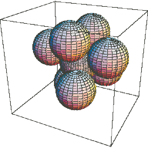
The preliminary results of Appendix A permit an attack on the solvation thermodynamics of hard core species built upon a simple device. Let’s consider a solute A that doesn’t interact with the solvent S molecules at all. We will consider formation of AS_n complexes and Fig. 1 depicts such a cluster. The interaction contribution $\beta\Delta\mu_{\mathrm{A}}$ is zero and the quasi-chemical Eq. 18 expresses

$$\ln\left[\left\langle\left\langle\prod\limits_{j}{(1-b_{\mathrm{A}j})}\right\rangle\right\rangle_{0}\right]=\ln x_{0}~.$$ (1)

But the left side here is a test particle average for solute that rigidly excludes solvent molecules from the region defined by the indicator function $b_{\mathrm{A}j}$. If the region is taken as defining a physically interesting molecule pair excluded volume, then the right side of Eq. 1 gives the negative of the excess chemical potential for the hard core solute defined by $b_{\mathrm{A}j}$. This is an example of the well known relation for hard core solutes $\ln p_{0}=-\beta\Delta\mu_{\mathrm{HC}}$ with ‘HC’ denoting ‘hard core’[9, 10, 11, 12, 13, 14, 15, 16, 17, 18, 19, 20, 3]. This observation sheds light on the compensation of inner and outer sphere contributions to the quasi-chemical Eq. 18 but is not surprising. We then consider ‘chemical’ equilibria for binding of S molecules to the A molecule. Of course, there is no interaction between the A molecule and the solvent molecules. The binding is just the occupancy by a solvent molecules of the ‘cavity’ defined by $b_{\mathrm{A}j}$. Combining these considerations gives

$$\beta\Delta\mu_{\mathrm{HC}}=\ln\left[{1+\sum\limits_{m\geq 1}K_{m}{}\rho_{\mathrm{S}}{}^{m}}\right]~.$$ (2)

The K_m are well-defined but typically computationally demanding; see Eq. 17. The evaluation of K${}_{m}{}^{(0)}$ will require few-body integrals over excluded volumes as is discussed in Appendix B. The primitive quasi-chemical approximation is

$$\beta\Delta\mu_{\mathrm{HC}}\approx\ln\left[1+\sum\limits_{m\geq 1}K_{m}{}^{(0)}\rho_{\mathrm{S}}{}^{m}\lambda{}^{m}\right]$$ (3)

with $\lambda$ a ‘mean field’ factor that achieves the self-consistency condition $\sum_{n}nK_{n}^{(0)}\rho_{\mathrm{S}}{}^{n}\lambda^{n}=\rho_{\mathrm{S}}K_{1}^{(0)}\sum_{n}K_{n}^{(0)}\rho_{\mathrm{S}}{}^{n}\lambda^{n}$. This amounts to an extension of the Poisson distribution for use in an information theory procedure[18]. Here $\rho_{\mathrm{S}}$K${}_{1}^{(0)}$=$<$n$>$ is the expected occupancy of the volume stenciled by $b_{\mathrm{A}j}$. Thus the multiplicative factors of $\rho_{\mathrm{S}}$ in $x_{n}^{(0)}\propto K_{n}{}^{(0)}\rho_{\mathrm{S}}{}^{n}$ are augmented by a self-consistent ‘mean field’ $\lambda$.

For reuse below, we summarize the technical results of this argument for hard core solutes, writing

$$\left\langle{\left\langle{e^{-\beta\Delta U_{\mathrm{HC}}}}\right\rangle}\right\rangle_{0}={1\over 1+\sum\limits_{m\geq 1}K_{m}{}\rho_{\mathrm{S}}{}^{m}}~.$$ (4)

This combines Eq. 2 and the potential distribution theorem Eq. 15 for this problem.

III Primitive Quasi-chemical Approximation

We can give a simple demonstration of the quantitative results of the primitive quasi-chemical theory by considering the hard disk (2d) and hard sphere fluids (3d). Table 1 gives Monte Carlo estimates of the K${}_{n}{}^{(0)}$ for those cases. The predicted distributions x_n for two densities are in Figs. 2 and 3. Equation of state results $\beta\Delta\mu(\rho)$ for these systems predicted by this primitive quasi-chemical theory are shown in Figs. 4 and 5. The primitive quasi-chemical approximation is remarkably successfully in all qualitative respects, particularly in view of its simplicity. In particular, the predicted occupancy distributions such as shown in Fig.  3 are remarkably faithful to the data. Nevertheless, the equation of state predictions begin progressively to incur serious quantitative errors at liquid densities $\rho d^{3}\!>$ 0.6, (Fig. 5).

Table 1: ‘Hit-or-Miss’ Monte Carlo estimates [22], as described in Appendix B, of $\ln$K${}_{n}{}^{(0)}$ for unit diameter hard spheres and disks, respectively. K${}_{1}{}^{(0)}$=${4\pi\over 3}$ ($\pi$) and K${}_{2}{}^{(0)}$=${17\pi^{2}\over 36}$ (${3\sqrt{3}\pi\over 8}$). The sample size was 24 G-configurations and the results are believed to be accurate to the number of significant figures given.

n	spheres (3d)	disks (2d)
1	1.43241	1.14473
2	1.53915	0.71321
3	0.56585	-1.190
4	-1.4697	-5.241
5	-4.684	-13.77
6	-9.168	-
7	-15.46	-

Figure 2: For the hard sphere fluid at $\rho_{\mathrm{S}}d^{3}$=0.277, comparison for n$\leq$5 of the Poisson distribution (solid curve) with primitive quasi-chemical distribution (dashed curve) implemented with the information theory constraint on the first moment $\sum nx_{n}=4\pi\rho_{S}d^{3}/3$. The dots are the results of Monte Carlo simulation[19] as discussed in Appendix D. The primitive quasi-chemical default model depletes the probability of high-n and low-n constellations and enhances the probability near the mode.

Figure 3: As in Fig. 2 but for $\rho_{\mathrm{S}}d^{3}$=0.8. The error bars indicate the statistical uncertainty by showing the 67% confidence interval.

Figure 4: $\beta\Delta\mu(\rho)$ for the two dimensional hard disk fluid on the basis of the primitive quasi-chemical approximation (dashed lined). The Ree-Hoover 3,3 Padé approximant[23] is the solid line and the dash-dot line is the first virial coefficient approximation.

Figure 5: $\beta\Delta\mu(\rho)$ for the three dimensional hard sphere fluid on the basis of the primitive quasi-chemical approximation (dashed line). The solid line is the prediction of the Carnahan-Starling equation of state, taken as the accurate basis for comparison, and the dash-dot line is the first virial coefficient approximation.

IV Test of the Equilibrium Ratios

As a direct check on the primitive quasi-chemical mechanism, we can focus on testing ideal populations Eq. 25 as approximations to formally correct populations Eq. 22. It is then natural to consider the ratios $x_{j}/x_{0}={K_{n}\rho_{\mathrm{S}}{}^{n}}$. Consideration of these ratios corresponds to shifting the curves of Figs. 2 and 3 so that the initial point is at the common value (0,1). A specific example is shown in Fig. 6. Compared with this normalization, it is clear that the observed equilibrium ratios K_n are greater than the ideal ratios K${}_{n}{}^{(0)}$.

Figure 6: $\ln\left[{(x_{n}/x_{0})_{qca}\over(x_{n}/x_{0})_{sim}}\right]$ vs. n comparing for the hard sphere fluid the primitive quasi-chemical approximate populations with those observed by Monte Carlo simulation for $\rho d^{3}$=0.8. This normalization focuses on the relative sizes of K_n and K${}_{n}{}^{(0)}$ suggesting that K${}_{n}\!>$K${}_{n}{}^{(0)}$ even after the maxent reweighting. The variations are modest except for the change between n=0 and n=1. The error bars indicate the statistical uncertainty by showing the 67% confidence interval. In the middle of the distribution the statistical uncertainty is mostly from the uncertainty in the denominator factor x₀.

V Correlations

A point of view here is that the geometric weighting with the $\lambda$’s of Eq. 3 establishes a mean field that adapts to the prescribed density. We now consider how to go beyond that mean field description. One idea is to extract the features of the summand of Eq. 4 that would give purely geometric weighting and then to analyze what remains. To this end, we define $\zeta=\exp(\beta\Delta\mu)$ and consult the formal identification of the equilibrium ratios Eqs. 17. Thus we can rewrite Eq. 4 as

$$\zeta=1+\sum_{m\geq 1}x_{0/m}K_{m}{}^{(0)}\zeta^{m}\rho_{\mathrm{S}}{}^{m}~,$$ (5)

with

$$x_{0/n}\equiv{\left\langle{\left\langle e^{-\beta\Delta U_{n}}\right\rangle}\right\rangle_{0}\over\left\langle e^{-\beta\Delta U}\right\rangle_{0}}~.$$ (6)

The remarkable Eq. 5 is formally exact and hasn’t been given before. The correlation factors $x_{0/m}$ might, in principle, be investigated on the basis of simulation data and information theory analysis. That is likely to a specialized nontrivial activity except of the lower density cases where the primitive quasi-chemical approximation is satisfactory.

V.1 Iterating the Quasi-Chemical Analysis

Alternatively, the quasi-chemical rules suggest natural theoretical approximation for the equilibrium ratios given formally by Eq. 17. Applying the rule Eq. 4, for n$>$0,

$$K_{n} = \left\langle{\left\langle e^{-\beta\Delta U_{n}}\right\rangle}\right\rangle_{0}K_{n}{}{}^{(0)}\zeta^{n+1}$$ (7)

$$= {K_{n}{}^{(0)}\zeta^{n+1}\over 1+\sum\limits_{m\geq 1}K_{m/n}\rho_{\mathrm{S}}{}^{m}}$$

$$\approx {K_{n}{}^{(0)}\zeta^{n+1}\over 1+\sum\limits_{m\geq 1}K_{m/n}{}^{(0)}\rho_{\mathrm{S}}{}^{m}}~.$$

The K_m/n can be understood by considering the chemical equilibrium

$$\mathrm{AS^{\prime}_{n}S_{m=0}\ +\ mS\rightleftharpoons AS^{\prime}_{n}S_{m}}~,$$ (8)

i.e. the original $\mathrm{AS^{\prime}_{n}}$ cluster is the solute and it provides a nucleus for a constellation of m S particles, different in type for the S^′ species. How to address the calculation of the K${}_{m/n}{}^{(0)}$ is discussed in Appendix C.

It is still helpful to focus on the populations even though more coefficients are involved now. To do this we consider

$$\zeta=1+\zeta\sum\limits_{m\geq 1}{\left\langle{\left\langle{e^{-\beta\Delta U_{m}}}\right\rangle}\right\rangle_{0}K_{m}{}^{(0)}\rho_{\mathrm{S}}{}^{m}\zeta^{m}}$$ (9)

and, to accomodate the additional factor of $\zeta$ multiplying the terms m$\geq$1, rearrange so that

$$\zeta=1+{{\sum\limits_{m\geq 1}{\left\langle{\left\langle{e^{-\beta\Delta U_{m}}}\right\rangle}\right\rangle_{0}K_{m}{}^{(0)}\rho_{\mathrm{S}}{}^{m}\zeta^{m}}}\over{1-\sum\limits_{m\geq 1}{\left\langle{\left\langle{e^{-\beta\Delta U_{m}}}\right\rangle}\right\rangle_{0}K_{m}{}^{(0)}\rho_{\mathrm{S}}{}^{m}\zeta^{m}}}}~.$$ (10)

This last equation is significant particularly because it suggests that a principal consequence of correlations can be a uniform reweighting of all coefficients m$\geq$1. Strikingly, that is exactly the suggestion of Fig. 6.

We can use this insight to push the argument further: the fact that the primitive quasi-chemical populations for m$\geq$1 are correct relative to each other means that the quantities $\left\langle{\left\langle{e^{-\beta\Delta U_{m}}}\right\rangle}\right\rangle_{0}$ are nearly exponentially dependent on m. For, in the first place, when the density is high, almost all the population is in the center of the distribution, and the Lagrange multipliers are negligibly affect by the relative reweighting of the m=0 term. Then the alteration of the original geometric weighting is literally irrelevant. In the second place, when the density is sufficiently low, these correlation factors are nearly unity anyway. So we can accurately write

$$\zeta\approx 1+A(\rho_{\mathrm{S}}{})\sum\limits_{m\geq 1}K_{m}{}^{(0)}\rho_{\mathrm{S}}{}^{m}\lambda{}^{m}~.$$ (11)

x₀ ‘breaks away’ from the rest of the distribution and requires individual consideration when the density is high enough that x₀ is sufficiently small due to correlation effects. Nevertheless

$$A(\rho_{\mathrm{S}}{})\approx{\zeta-1\over\zeta_{0}-1}~,$$ (12)

where $\zeta_{0}$ is the primitive quasi-chemical approximate value. Thus, when the primitive quasi-chemical approximation is sufficiently accurate, the difficulty of evaluating the corrections should be much reduced.

Though it would be interesting to calculate correlation corrections on the basis of Eq. 7 and Appendix C, a simpler, empirical approach suffices for our present purposes. This is because the discrepancies seen in Fig. 5 are substantial but not problematic and, therefore, the required A($\rho_{\mathrm{S}}{}$) is simple. In particular, the form

$$\beta\Delta\mu=\ln\left({1+e^{7.361\rho_{\mathrm{S}}{}^{4}}\sum\limits_{m\geq 1}{K_{m}{}^{(0)}\rho_{\mathrm{S}}{}^{m}\lambda{}^{m}}}\right)$$

(13)

conforms accurately to the Carnahan-Starling equation of state; see Fig. 7. The literal coefficient in Eq. 13 was obtained by fitting on the basis of the Eq. 12 to minimize the discrepancy with the Carnahan-Starling equation of state.

Figure 7: Equation of state with the empirical correlation model, Eq. 13. (Lower panel) The solid line is the Carnahan-Starling equation of state and the dashed line is the model of Eq. 13. (Upper panel) Discrepancy: the empirical correlation model (Eq. 13) less the Carnahan-Starling value. The mean absolute discrepancy against Carnahan-Starling equation of state is about 1% and the maximum discrepancy is less than 3%, nearly as good conformance to the Carnahan-Starling model as that model to simulation data. When the final empirical parameter was fitted using only $\rho_{\mathrm{S}}d^{3}\leq$ 0.3, the mean absolute discrepancy hardly changed but the maximum discrepancy doubled.

The occupancies predicted by this empirical model are depicted in Fig. 8.

Figure 8: Predicted occupancies with the empirical correlation model, Eq. 13, for $\rho_{\mathrm{S}}d^{3}$=0.8. Compare to Fig. 3. Again the solid line is the Poisson distribution.

VI Concluding Discussion

Our first goal was to work-out how the quasi-chemical theory, a fresh attack on the the statistical thermodynamic theory of liquids, applies to the paradigmatic hard sphere fluid. The second goal was to work-out theoretical approximation procedures that might assist in describing dense liquids of non-spherical species. The new fundamental results here apply generally to ‘hard core’ molecular models. The primitive quasi-chemical approximation, the procedure for iterating the quasi-chemical analysis, and the recognition of the ‘break away’ phenomenon of Fig. 6 are likely to be helpful in understanding packing in dense molecular liquids, beyond the hard sphere fluid. For the hard sphere system specifically, we have obtained a simple occupancy model, Eq 13, that is likely to be helpful in a variety of other situations.

One situation is the description of packing restrictions when the quasi-chemical theory is used to treat genuinely chemical interactions, for example in the study of hydration of atomic ions in water[24, 25]. The issue of ‘context hydrophobicity’ associated with many molecular solutes, including molecular ions, in water can also be addressed on the basis of quasi-chemical calculations and the developments here.

Another situation of current interest is the theory of primitive hydrophobic effects that has recently been reborn[9, 10, 11, 12, 13, 14, 15, 16, 17, 18, 19, 20, 3]. An historical view has been that the initial issue of hydrophobic effects was the hydration structures and thermodynamics following from volume exclusion by nonpolar molecules in liquid water. The balance of attractive forces that might produce drying phenomena was a secondary concern, except that ‘drying’ was always present in the scaled particle models[26]. With the convincing clarification of the first of these problems[9, 10, 11, 12, 13, 14, 15, 16, 17, 18, 19, 20, 3], the issue of drying phenomena has been now taken up more enthusiastically[27, 28, 3]. In this context, we note that the striking success of the two-moment information models and the Pratt-Chandler theory[9, 10, 11, 12, 13, 14, 15, 16, 17, 18, 19, 20, 3, 29] is due, in part, to a fortuitous balance of a ‘gaussian’ approximation in the theory[18] and a compensating disregard for drying possibilities[30]; both of these compensating approximations are expected to be benign for small molecule solutes. One ingredient in a better understanding of this situation is a careful solution to the case where drying phenomena are entirely absent. That ingredient is better in hand with the results above.

Appendix A Preliminary Results

A.1 Potential Distribution Theorem

The potential distribution theorem[14, 1, 2, 31] may be expressed as

$$\rho_{\sigma}=\left\langle{\left\langle{e^{-\beta\Delta U}}\right\rangle}\right\rangle_{0}z_{\sigma}\left({q_{\sigma}/V}\right)$$ (14)

where $\rho_{\sigma}$ is the density of molecules of type $\sigma$ (the ‘solute’ under consideration), $z_{\sigma}=\exp(\beta\mu_{\sigma})$ is the absolute activity of that species, q_σ is the single molecule partition function for that species, and V is the volume. The double brackets $\left<\left<\ldots\right>\right>_{0}$ indicate the average over the thermal motion of the solute and the solvent under the conditions of no interaction between them, and the averaged quantity is the Boltzmann factor of those interactions. The average indicated here is the ratio of the activity of an isolated solute, $\rho_{\sigma}V/{q_{\sigma}}$, divided by the absolute activity, $z_{\sigma}$, of the actual solute. Thus

$$\beta\mu_{\sigma}=\ln\left[{V\rho_{\sigma}\over\left\langle{\left\langle{e^{-\beta\Delta U}}\right\rangle}\right\rangle_{0}q_{\sigma}}\right]~.$$ (15)

This is a formal result to the extent that evaluation of the quantities on the right side typically will involve nontrivial calculations on many-body systems.

A.2 Chemical Equilibrium

The traditional chemical thermodynamic consideration of a chemical transformation such as

$$\mathrm{n_{\mathrm{A}}A+n_{\mathrm{B}}B\rightleftharpoons n_{\mathrm{C}}C+n_{\mathrm{D}}D}$$ (16)

with the formal result of Eq. 15 leads to the formal expression

$$K \equiv {\rho_{\mathrm{C}}{}^{n_{\mathrm{C}}}\rho_{\mathrm{D}}{}^{n_{\mathrm{D}}}\over\rho_{\mathrm{A}}{}^{n_{\mathrm{A}}}\rho_{\mathrm{B}}{}^{n_{\mathrm{B}}}}$$ (17)

$$= {\left(\left\langle\left\langle e^{-\beta\Delta U_{\mathrm{C}}}\right\rangle\right\rangle_{0}{q_{\mathrm{C}}\over V}\right){}^{n_{\mathrm{C}}}\left(\left\langle\left\langle e^{-\beta\Delta U_{\mathrm{D}}}\right\rangle\right\rangle_{0}{q_{\mathrm{D}}\over V}\right){}^{n_{\mathrm{D}}}\over\left(\left\langle\left\langle e^{-\beta\Delta U_{\mathrm{A}}}\right\rangle\right\rangle_{0}{q_{\mathrm{A}}\over V}\right){}^{n_{\mathrm{A}}}\left(\left\langle\left\langle e^{-\beta\Delta U_{\mathrm{B}}}\right\rangle\right\rangle_{0}{q_{\mathrm{B}}\over V}\right){}^{n_{\mathrm{B}}}}~.$$

This should be compared to the textbook result for ideal gas systems[32]. That comparison shows that the single molecule partition functions are multiplicatively augmented by the test particle averages. But otherwise the structure of this important result is unchanged. The conclusion here is that the equilibrium ratios are well-defined objects though formal to the extent that nontrivial computational effort would be required to evaluate them on the basis of molecular information.

A.3 Quasi-chemical Theory

The quasi-chemical develop starts from consideration of a distinguished molecule in the solution and seeks to evaluate the chemical potential on the basis of events occurring within a defined ‘inner sphere.’ For a species of type A, that definition is codified by specifying a function $b_{\mathrm{A}j}$ that is equal to one (1) when solution molecule j is inside the defined region and zero (0) otherwise. Our starting point can be [2]

$$\beta\Delta\mu_{\mathrm{A}} = \ln x_{0}$$ (18)

$$- \ln\left[\left\langle\left\langle{e^{-\beta\Delta U_{\mathrm{A}}}}\prod\limits_{j}{(1-b_{\mathrm{A}j})}\right\rangle\right\rangle_{0}\right],$$

where $x_{0}$ is the fraction of A solute species with zero (0) neighbors in the defined region. $\Delta U_{\mathrm{A}}$ is the interaction energy of the solvent with the solute A that is treated as a test particle. The potential distribution theory perspective on Eq. (18) is

$$x_{0} = \left\langle\prod\limits_{j}{(1-b_{\mathrm{A}j})}\right\rangle$$ (19)

$$= {\langle\langle{e^{-\beta\Delta U_{\mathrm{A}}}}\prod\limits_{j}{(1-b_{\mathrm{A}j})}\rangle\rangle_{0}\over\langle\langle{e^{-\beta\Delta U_{\mathrm{A}}}}\rangle\rangle_{0}}.$$

The first, or chemical term, of Eq. 18 can be analyzed with chemical concepts associated with the reactions

$$\mathrm{AS_{n=0}\ +\ nS\rightleftharpoons AS_{n}}$$ (20)

Here the indicated complexes are composed of $n$ solvent (S) molecules within the defined region. Remember that the A molecule is a ‘distinguished’ solute molecule considered at the lowest non-zero concentration [1]. The fractional amount of A species with a given solvation number $n$ can be described by a chemical equilibrium ratio

$$K_{n}={\rho_{\mathrm{AS_{n}}}\over\rho_{\mathrm{AS_{n=0}}}\rho_{\mathrm{S}}{}^{n}}~.$$ (21)

The $\rho_{\sigma}$ are the number densities and, in particular, $\rho_{\mathrm{S}}$ is the bulk number density of solvent molecules since the distinguished A molecule is infinitely dilute. This notation permits the normalized re-expression

$$x_{n}={{K_{n}\rho_{\mathrm{S}}{}^{n}}\over{1+\sum\limits_{m\geq 1}{K_{m}\rho_{\mathrm{S}}{}^{m}}}}.$$ (22)

Since this yields

$$x_{0}{}^{-1}={1+\sum\limits_{m\geq 1}{K_{m}\rho_{\mathrm{S}}{}^{m}}},$$ (23)

the original Eq. (18) can be re-expressed as

$$\beta\Delta\mu_{\mathrm{A}} = -\ln\left[1+\sum\limits_{m\geq 1}{K_{m}\rho_{\mathrm{S}}{}^{m}}\right]$$ (24)

$$-\ln\left[\left\langle\left\langle{e^{-\beta\Delta U}}\prod\limits_{j}{(1-b_{\mathrm{A}j})}\right\rangle\right\rangle_{0}\right].$$

The virtue of these rearrangements is that the natural first approximation is

$$x_{n}\approx x_{n}{}^{(0)}={{K_{n}{}^{(0)}\rho_{\mathrm{S}}{}^{n}}\over{1+\sum\limits_{m\geq 1}{K_{m}{}^{(0)}\rho_{\mathrm{S}}{}^{m}}}}.$$ (25)

The K${}_{n}{}^{(0)}$ are equilibrium ratios for the chemical reaction (20) in an ideal gas. This formulation and the approximation of Eq. (25) are closely related [2] to the quasi-chemical (or cluster-variation) approximations of Guggenheim [33], Bethe [34], and Kikuchi [35].

This approach should have greatest utility where the chemical balances of Eq. 20 are dominated by inner sphere chemistry that can be captured with computations on clusters. Such chemical interactions are often much larger than the outer sphere contribution, the right-most term of Eq. 18.

But that outer sphere contribution remains and can’t be neglected forever. An interesting example based on simulation of liquid water was discussed recently[3]. There the x₀ was estimated from molecular dynamics results and the remainder, the outer-sphere contributions to $\beta\Delta\mu$, were positive, suggesting domination of those outer-sphere contributions by the packing constraints studied here. A principal goal of the present work is the development of a reasonable approach for describing the packing issues necessary for treating those outer sphere contributions.

Reiss and Merry[36] analyzed population relations analogous to Eq. 22 but with activities appearing in the place of densities and with coefficients, here the equilibrium ratios K_n, appropriately different. The additional formal point here is the replacement of the activity by the density that permits the identification of the K_n in Eq. 2, and then further permits consideration of the mean field treatment Eq. 3 on the basis of an information theory constraint when K${}_{n}{}^{(0)}$ will be used. At this stage, the quasi-chemical approximation achieves a particularly primitive character and deviates from the goal of bounding these thermodnamic quantities that was pursued by Reiss and Merry[36].

Appendix B Calculation of the K${}_{n}{}^{(0)}$ for hard spheres and hard disks

The K${}_{n}{}^{(0)}$ sought for reaction Eq. 20 are given by

$$K_{n}{}^{(0)}={{q_{\mathrm{AS_{n}}}}\over\left({q_{\mathrm{S}}/V}\right)^{n}{q_{\mathrm{AS_{n=0}}}}}~.$$ (26)

(See Eq. 17.) For this problem, $q_{\mathrm{S}}=V/\Lambda_{S}{}^{3}$ with $\Lambda_{S}$ a thermal deBroglie wavelength for S but these momentum integrals cancel perfectly and are irrelevant as usual. Therefore,

$$n!K_{n}^{(0)}=\int\limits_{A}{d^{3}r_{1}\ldots\int\limits_{A}{d^{3}r_{n}\left({\prod\limits_{j>i=1}^{n}{e(i,j)}}\right)}}~.$$ (27)

The notation $\int_{A}{d^{3}r_{k}}$ indicates the three-dimensional spatial integral over the volume of the A-ball, a sphere of radius 1. The indicated integrand is thus 3n dimensional. The integrand is zero (0) if $|\bf{r}_{i}-\bf{r}_{j}|<1$ (overlap) for any (ij) and one (1) otherwise. Thus the integral can be estimated by sampling n-point uniform placments in the A-ball and scoring the fraction of such placements that are free from overlaps between the n unit diameter S-spheres. This approach fails for n larger than those presented in Table 1. But larger clusters were not observed in our simulation of the fluid, so our approach should be regarded as satisfactory.

The analogous two dimensional procedure was used for the hard disk results.

Appendix C Calculation of the K${}_{m/n}{}^{(0)}$

In contrast to Appendix B, here the ratio sought is

$$K_{m/n}{}^{(0)}={{q_{\mathrm{AS_{n}^{\prime}S_{m}}}}\over\left({q_{\mathrm{S}}/V}\right)^{m}{q_{\mathrm{AS_{n}^{\prime}}}}}~,$$ (28)

corresponding to the reaction Eq. 8. Again, the explicit factors of V, the momentum integrals, and the factor of $n!$ all cancel perfectly so that

$$m!K_{m/n}^{(0)}=\left\langle{\int\limits_{AS^{\prime}_{n}}{d^{3}r_{1}\ldots\int\limits_{AS^{\prime}_{n}}{d^{3}r_{m}\left({\prod\limits_{j>i=1}^{m}{e(i,j)}}\right)}}}\right\rangle~.$$

(29)

Here the notation $\int_{AS_{n}^{\prime}}{d^{3}r_{k}}$ indicates an integral over the excluded volume of an AS${}_{n}^{\prime}$ complex to an S ligand. The SS excluded volume, the integrand, is the same as before. But the structure of the AS${}_{n}^{\prime}$ complex fluctuates and the volumes obtained for specific structures are averaged over these fluctuations. The brackets $\langle\ldots\rangle$ indicate the average over the structures of the isolated AS${}_{n}^{\prime}$ complex. This averaging is permitted and governed by the non-trivial denominator that appears in Eq. 28.

Operationally, the calculation can be much as in Appendix B except for (a) averaging utlizing a Metropolis Monte Carlo calculation for the n ligand spheres in the star AS${}_{n}^{\prime}$; and (b) random placements of the m additional points are into a sphere of radius two (2) since that would fully enclose any conformation of the cluster.

Appendix D Calculation of x_n for the Hard Sphere Fluid

The probability that there are $\mathrm{n-1}$ points in a sphere of radius $r$, x${}_{n-1}(r)$, can be obtained from the distribution, $4\pi\rho_{S}r^{2}\mathcal{D}_{n}(r)$, of the distance $r$ to the nth nearest neighbor of an arbitrary point. The probability that there are no more than $\mathrm{n-1}$ molecules in the void is equal to the probability that the nth nearest neighbor is at least $r$ away from the void center

$$\sum_{m=0}^{n-1}x_{m}(r)=4\pi\rho_{S}\int_{r}^{\infty}\mathcal{D}_{n}(y)y^{2}dy~.$$ (30)

Isobaric-isothermal Monte Carlo can be used to calculate $\mathcal{D}_{n}(r)$. x${}_{n}(r)$ for a range of $r$ can be obtained from the distributions $\mathcal{D}_{n}(r)$. To increase the accuracy of the estimated $\mathcal{D}_{n}(r)$ for rarely observed $r$, small and large, a specific point in the simulation volume was chosen, and the sampling probability was reweighted by $\left[4\pi\rho_{\mathrm{S}}r_{1}{}^{2}e^{-4\pi\rho_{\mathrm{S}}r_{1}{}^{3}/3}+C\right]^{-1}$ where $r_{j}$ is the distance from the chosen point to the jth nearest center for each configuration and C is an empirically chosen, dimensional constant. This importance sampling

$$4\pi\rho_{S}r^{2}\mathcal{D}_{n}(r)={\left<\left[4\pi\rho_{\mathrm{S}}r_{1}{}^{2}e^{-4\pi\rho_{\mathrm{S}}r_{1}{}^{3}/3}+C\right]\delta(r-r_{n})\right>\over\left<\left[4\pi\rho_{\mathrm{S}}r_{1}{}^{2}e^{-4\pi\rho_{\mathrm{S}}r_{1}{}^{3}/3}+C\right]\right>}$$ (31)

is based upon the idea that $\mathcal{D}_{1}^{(0)}(r)=e^{-4\pi\rho_{\mathrm{S}}r^{3}/3}$ is the function[37] appropriate for a random distribution of spheres. This idea attempts to make the observed distribution of the distance to the nearest particle more nearly uniform. The constant C was included to avoid an unbounded weighting function. The denominator of Eq. D2 is just a normalizing factor on the distribution. The denominator of Eq. 31 merely provides a normalizing factor.

Isobaric-isotermal ensembles of 108 and 256 hard spheres were sufficient. The Carnahan-Starling equation was used to find the $\beta$p needed for a hard sphere simulation at each specific density.

References

- [1] L. R. Pratt and R. A. LaViolette, Mol. Phys. 94, 909 (1998).
- [2] L. R. Pratt and S. B. Rempe, in Simulation and Theory of Electrostatic Interactions in Solution. Computational Chemistry, Biophysics, and Aqueous Solutions, edited by L. R. Pratt and G. Hummer (American Institute of Physics, Melville, NY, 1999), vol. 492 of AIP Conference Proceedings, pp. 172–201.
- [3] G. Hummer, S. Garde, A. E. García, and L. R. Pratt, Chem. Phys. 258, 349 (2000).
- [4] D. Chandler, J. D. Weeks, and H. C. Andersen, Science 220, 787 (1983).
- [5] A. R. Altenberger and J. S. Dahler, Phys. Rev. E 54, 6242 (1996).
- [6] M. Robles, M. L. deHaro, A. Santos, and S. B. Yuste, J. Chem. Phys. 108, 1290 (1998).
- [7] L. V. Yelash, T. Kraska, and U. K. Deiters, J. Chem. Phys. 110, 3079 (1999).
- [8] G. Parisi and F. Slanina, Phys. Rev. E 62, 6554 (2000).
- [9] A. Pohorille and L. R. Pratt, J. Am. Chem. Soc. 112, 5066 (1990).
- [10] L. R. Pratt and A. Pohorille, Proc. Natl. Acad. Sci. USA 89, 2995 (1992).
- [11] L. R. Pratt and A. Pohorille, in Proceedings of the EBSA 1992 International Workshop on Water-Biomolecule Interactions, edited by M. U. Palma, M. B. Palma-Vittorelli, and F. Parak (Societá Italiana de Fisica, Bologna, 1993), pp. 261–268.
- [12] G. Hummer, S. Garde, A. E. García, A. Pohorille, and L. R. Pratt, Proc. Natl. Acad. Sci. USA 93, 8951 (1996).
- [13] S. Garde, G. Hummer, A. E. García, M. E. Paulaitis, and L. R. Pratt, Phys. Rev. Lett. 77(24), 4966 (1996).
- [14] L. R. Pratt, Encyclopedia of Computational Chemistry (John Wiley & Sons, Chichester, 1998), pp. 1286–1294, hydrophobic effects.
- [15] G. Hummer, S. Garde, A. E. García, M. E. Paulaitis, and L. R. Pratt, Proc. Natl. Acad. Sci. USA 95, 1552 (1998).
- [16] G. Hummer, S. Garde, A. E. Garcia, M. E. Paulaitis, and L. R. Pratt, J. Phys. Chem. B 102, 10469 (1998).
- [17] A. Pohorille, Pol. J. Chem. 72, 1680 (1998).
- [18] L. Pratt, G. Hummer, and S. Garde, in New Approaches to Problems in Liquid State Theory, edited by C. Caccamo, J.-P. Hansen, and G. Stell (Kluwer, Netherlands, 1999), vol. NATO Science Series 529, pp. 407–420.
- [19] M. A. Gomez, L. R. Pratt, G. Hummer, and S. Garde, J. Phys. Chem. B 103, 3520 (1999).
- [20] S. Garde, A. E. Garcia, L. R. Pratt, and G. Hummer, Biophys. Chem. 78, 21 (1999).
- [21] G. E. Crooks and D. Chandler, Phys. Rev. E 56(4), 4217 (1997).
- [22] J. M. Hammersley and D. C. Handscomb, Monte Carlo Methods (Chapman and Hall, London, 1964).
- [23] F. H. Ree and W. G. Hoover, J. Chem. Phys. 40, 939 (1964).
- [24] S. B. Rempe, L. R. Pratt, G. Hummer, J. D. Kress, R. L. Martin, and A. Redondo, J. Am. Chem. Soc. 122, 966 (2000).
- [25] S. B. Rempe and L. R. Pratt, Fluid Phase Equilibrium xxx, yyy (2001), in press, LA-UR-00-2309, http://xxx.lanl.gov/abs/physics/0006026.
- [26] F. H. Stillinger, J. Soln. Chem. 2, 141 (1973).
- [27] G. Hummer and S. Garde, Phys. Rev. Letts. 80, 4193 (1998).
- [28] K. Lum, D. Chandler, and J. D. Weeks, J. Phys. Chem. B 103, 4570 (1999).
- [29] L. R. Pratt and D. Chandler, J. Chem. Phys. 67, 3863 (1977).
- [30] L. R. Pratt and D. Chandler, J. Chem. Phys. 73, 3434 (1980).
- [31] B. Widom, J. Phys. Chem. 86, 869 (1982).
- [32] D. A. McQuarrie, Statistical Mechanics (Harper & Row, New York, 1976), chapter 9.
- [33] E. A. Guggenheim, Proc. Rov. Soc. London A 148, 304 (1935).
- [34] H. Bethe, Proc. Rov. Soc. London A 150, 552 (1935).
- [35] S. G. Brush and R. Kikuchi, Lattice Models for Cooperative Phenomena. I. Survey and Comparison of Approximate Methods, Tech. Rep. UCRL-14287, University of California, Lawrence Radiation Laboratory, Livermore, CA (1965).
- [36] H. Reiss and G. A. Merry, J. Phys. Chem. 85, 3313 (1981).
- [37] S. Chandrasekhar, Rev. Mod. Phys. 15, 1 (1943).