

Reversible maps and composites of involutions in groups of piecewise linear homeomorphisms of the real lineThanks: This second author’s work was supported by Science Foundation Ireland grant 05/RFP/MAT0003.
Abstract.
Making use of techniques developed by Brin and Squier, we compare results of Fine and Schweigert, Jarczyk and Young about reversibility and composites of involutions in the group of homeomorphisms of the real line with similar results for groups of piecewise linear homeomorphisms of the real line.
Key words and phrases:
Reversible, involution, piecewise linear.2000 Mathematics Subject Classification
Primary 37E05, 57S05. Seconday 57S251. Introduction
1.1. The background of reversibility
A member of a group is reversible if it is conjugate to its own inverse within , and is strongly reversible if it is reversible and the conjugating map can be chosen to be an involution. The purpose of this paper is to study the reversible and strongly reversible elements of groups of piecewise linear homeomorphisms of the real line.
Interest in reversibility originates from the theory of dynamical systems. For example, Birkhoff ([Bir15]) used time-reversible symmetry in his study of the three body problem, and Arnol’d and Sevryuk ([AS86]) identified reversible dynamical systems that are not strongly reversible. (See [LR98] for many more references.)
In finite group theory, reversible and strongly reversible elements of groups are described as real and strongly real. This terminology is used because an element of a finite group is reversible if and only if the image of under each irreducible character of is real. The strongly reversible elements of a finite group can also be determined from the character table of , provided that the conjugacy classes of involutions in are known ([Isa94]). Problem 14.82 of the Kourovka Notebook ([KN05]) is to classify those finite simple groups which consist entirely of strongly reversible elements, and there has been progress on this problem ([MKe02, TZ05]).
Recently, Jarczyk and Young ([Jar02b, You94]) classified the strongly reversible maps in the group of homeomorphisms of the real line. Related results about composites of involutions in the group of homeomorphisms of the real line can be found in [FS55, Jar02a, MS85, O’F04]. In this paper we compare the results of Fine and Schweigert, Jarczyk and Young with similar results about groups of piecewise linear homeomorphisms of the real line.
1.2. Formal definition of reversibility
Let be a group. An element in is reversible if and only if there is an element in such that . We say that reverses . Let denote the identity element of . An involution in is an element such that . An element in is strongly reversible if and only if there is an involution such that . Notice that is strongly reversible if and only if there are involutions and such that . Define
for . Then
The set consists of the involutions in , and consists of the strongly reversible members of . The limit of this chain of subsets is a normal subgroup denoted ; it is the subgroup of generated by involutions. Likewise we define
for . Again we have a chain
and the limit, , is a normal subgroup of . Membership of and is preserved under conjugation.
In this paper we examine the sets and for groups described in the next section. For brevity, we often describe the purpose of this paper—the classification of the sets and —as a classification of reversibility.
1.3. The groups of interest
Primarily, we consider reversibility in three groups.
- (i)
The full group of homeomorphisms of the real line, denoted .
- (ii)
The group of homeomorphisms of which are locally affine at all but a finite number of points of .
- (iii)
The group of homeomorphisms of which are locally affine at all but a discrete set of points of .
The points at which piecewise linear functions are not locally affine are called nodes.
Each of these groups has a subgroup of index which is also of interest: the subgroup of orientiation preserving (strictly increasing) maps. We denote these three subgroups , and . Each subgroup has a coset of orientation reversing maps, and we denote these cosets , and .
The sets and defined in §1.2 will be described for these six groups. In addition, we often refer to a number of other subgroups of , without such a comprehensive analysis of reversibility. For example, we consider the group of differeomorphisms (smooth homeomorphisms) of , and the group of real analytic homeomorphisms of . We look at the subgroup of which consists of functions for which there is a positive number such that whenever . Also, we study the subgroup of homeomorphisms in with compact support.
1.4. The structure of the paper
A map is reversible if and only if it lies in the same conjugacy class as its inverse. Therefore a fundamental step in our classification of reversibility is a classification of conjugacy. Such a classification appears in §2. Much of this material is unoriginal. A description of conjugacy in can be found in [Gla81] or [O’F04]. Our discussion of the conjugacy classes of is taken from [BS01]. We provide clear details if not proofs of the conjugacy classification in because [BS01] is difficult to decipher. The rest of §2 is about conjugacy in , and other similar groups. This material has not, to our knowledge, been published before although Brin and Squier, amongst others, were no doubt aware of it.
An element of a group may not be reversible as an element of , but it might be reversible when considered in a group containing . This situation arises when conjugacy classes of are found to fuse in . Such fusion is induced by outer automorphisms of hence, to examine fusion (and therefore give a complete description of reversibility), we must examine the outer automorphisms of . Since , and have trivial centres we may consider each of them as normal subgroups of their full automorphism group; fusion must therefore occur inside this full automorphism group. In §3 we examine the automorphism groups and normal subgroups of , and . This ensures that we consider reversibility in both a broader and narrower context. The material in §3 is well known.
With the exception of a few results due to Fine and Schweigert, Jarczyk and Young (which are stated and referenced, but not proved) all the results of §4, §5, §6 and §7 are original. In §4 we classify reversibility. In §5 we determine for and one of our homeomorphism groups. Then in §6 we characterise the strongly reversible maps, and compare strong reversibility with reversibility. Finally, in §7 we study the classes .
Each section is structured similarly; the first three subsections are devoted to the groups , and and their orientation preserving subgroups. The final subsection is about other subgroups of which may be of interest.
1.5. Summary of results
We summarise certain primary results here for comparison and convenience.
Section 4 is about reversibility. The reversible elements of , and are determined from the description of conjugacy classes in §2. Both groups and contain reversible maps. In contrast, does not contain any non-trivial reversible maps.
Section 5 is about composites of reversible maps. Our findings are summarised in the next theorem.
Theorem 1.1.
We have
- (i)
and ;
- (ii)
and for each ;
- (iii)
and .
Section 6 is about strong reversibility. There are no orientation preserving non-trivial involutions in . Hence our study of strong reversibility and the sets is worthwhile only if we include the coset of orientation reversing homeomorphisms (so, for example, we work in rather than ). The next theorem is about the contrast between reversibility and strong reversiblity in the , and . (Part (i) of Theorem 1.2 follows from [You94, Theorem 2.2].)
Theorem 1.2.
- (i)
In , an orientation preserving reversible map is strongly reversible if and only if it is reversed by an orientation reversing homeomorphism.
- (ii)
In , reversibility and strong reversibility are equivalent.
- (iii)
In , an orientation preserving reversible map is strongly reversible if and only if it is reversed by an orientation reversing homeomorphism.
Note that, because the composite of two non-trivial involutions is orientation preserving, the only orientation reversing strongly reversible homeomorphisms are involutions.
Section 7 is about composites of involutions. A key result is summarised in the next theorem. (Part (i) of Theorem 1.3 is the same as [FS55, Theorem 6], [Jar02b, Theorem 2] and [O’F04, Theorem 3.2].)
Theorem 1.3.
We have
- (i)
and ;
- (ii)
;
- (iii)
and .
1.6. Notation
Typically we reserve uppercase Roman letters such as , and for groups or sets. Similarly lowercase letters such as , , and are elements of our groups (and so tend to be homeomorphisms of the real line), while lowercase letters such as , and are elements in the domain of these functions, . There is a partial order on the set of all continuous functions on given by if and only if for all . If and then we write . Typically our functions are members of homeomophism groups so we write for the composition of followed by . When a homeomorphism is composed with, for example, a function , we denote the resulting composite function .
For elements , and of a group we will write for . We will also write to mean that there exists such that , that is, and are conjugate as elements of . All functions will act on the left.
We reserve particular lower-case Greek letters for specific functions. The letters and always denote involutions. The identity function will be denoted . The function that maps to for each real number will be denoted . We write simply as . Upper-case Greek letters will typically be used to denote conjugacy invariants.
For a function and a point we will denote the left and right derivatives of at , provided they exist, by and . The fixed point set of , which is a closed subset of , is denoted .
2. Conjugacy
We discuss the conjugacy classes of our groups of interest. Of course, many properties of are inherited by the subgroups and .
2.1. Conjugacy in H
For details of the conjugacy classification in , see [FS55, Gla81, O’F04]. We state the key results without proof.
Define the degree of , denoted , to be if , and if . For we define the signature of as follows: where
Conjugacy in both groups and can be understood in terms of the following two propositions ([O’F04, Lemma 2.3 and Lemma 2.4]).
Proposition 2.1.
Given maps , there is a map such that if and only if there is a map in such that .
Proposition 2.2.
Two maps are conjugate in if and only if there is a map in that maps the fixed point of to the fixed point of such that .
All the orientation preserving maps in other than the identity are of infinite order. The fixed points sets are closed subsets of . The orientation reversing maps in are either of order two (involutions) or else of infinite order. Each orientation reversing map has exactly one fixed point. The involutions can be characterised as those maps whose graph is symmetric about the line . Notice that, by Proposition 2.2, all maps of order two are conjugate to each other.
2.2. Conjugacy in PLF
2.2.1. Conjugacy in
We begin by considering maps and describing the conditions under which . We summarise the results of Brin and Squier ([BS01]) which describe the conjugacy classes in . They do this by means of three geometric invariants of conjugate elements in , denoted , and , which characterise the conjugacy classes—so any two distinct conjugacy classes must take different values on at least one of these invariants.
For the purpose of illustrating these results we consider the same example throughout. Let be the unique member of such that
and the only turning points in the graph of (shown in Figure 1) occur at , , , , and .
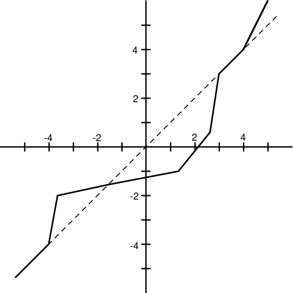
For , define
The set consists of points where the graph of diverges from the graph of , and consists of a union of open intervals which we will call the small domains of .
The first conjugacy invariant of concern is , as already defined for . This invariant simplifies significantly in because changes value only a finite number of times. For our example:
In the group (and likewise in the group ), it is more illuminating to consider merely as an ordered list of integers , and corresponding to the values taken by on the small domains. No essential information is lost in representing in this way because, by conjugating by maps in , we can adjust the size (but not the order) of the small domains of . Thus, for our example, .
Next, for each small domain let be the smallest node of , supposing such a point exists. If no such point exists then let be an arbitrary element of . Define to be the ordered list of values taken on by . So, for our example, .
Finally, is going to be an ordered list of equivalence classes of functions , one for each small domain . Let represent with the points and identified. Each will be a function from to the positive real numbers which takes the value at all but a finite number of points in .
We define a bump domain of to be a small domain such that over ; this corresponds to a bump in the graph of away from the line . For small domains that are not bump domains we require that all are identical, so we arbitrarily choose that is the function which takes the value for each point in .
Now suppose that is a bump domain. First define a function :
The graph of these functions will depart from the graph of over the domain only, that is, it will have exactly one bump. For our example, the graph of is shown in Figure 2.

Next we define a second function . We define first for the case where takes the value on , meaning that the bump over lies above as in Figure 2. For , let
The orbit intersects in precisely one point. Define to consist of those members of that are nodes of . This set is finite. Let
When then and we define .
Note that will take the value outside . For our example, the graph of is shown in Figure 3.

It remains to define . Let denote the group of orientation preserving affine homeomorphisms of . Let be the unique member of that coincides with on . If the gradient of is not equal to and has fixed point , then ; otherwise, if , then for some . The map can be embedded in a flow in , where
Define by .
Let denote the set of all functions from to that take the value 1 for all but finitely many points in . Then . Two maps are equivalent if there is a translation , with , such that . Write for the equivalence class of .
We define to be the ordered list of equivalence classes of functions where is a small domain of . For our example we have
For a function define . We summarise [BS01, Theorem 5.3].
Proposition 2.3.
Two homeomorphisms and in are conjugate if and only if .
2.2.2. Conjugacy in
We consider and describe the conditions under which . Observe that can be decomposed into two cosets and where satisfies for each .
We can immediately make the following statement.
Proposition 2.4.
Two orientation preserving maps in are conjugate if and only if or .
To characterise conjugacy we need to explain what the invariants , and look like. After conjugation by , the graph of is rotated by an angle about the origin. Thus if then . Also, because the final line segment of a bump domain of is the initial line segment of a bump domain of , we see that consists of a list of slopes of final line segments of small domains of , listed in reverse order.
Finally, define a map by and define a map in an analagous manner to the definition of , but with the largest rather than smallest node of , and with unique member of that coincides with on . Then is a list of equivalence classes of functions for small domains of , listed in reverse order.
A summary of the values of is given in Table 1. In the table are the small domains of , is the slope of the initial line-segment of the graph of over and is the slope of the final line-segment of the graph of over . Note that the table includes values for ; this will be relevant in the next section when we study reversibility.
We are left with the question of conjugacy amongst orientation reversing homeomorphisms. The result is comparable to the result for .
Proposition 2.5.
Let . Then is conjugate to in if and only if there is that maps the fixed point of to the fixed point of such that .
Proof.
One implication is straightforward. For the converse implication, let have fixed point , let have fixed point , and suppose that there is such that and . By replacing with if necessary, we can assume that . Define by
Then . ∎
Hence all involutions in are conjugate in .
2.3. Conjugacy in PL
Conjugacy in bears a strong resemblance to that in .
2.3.1. Conjugacy in
As for we define small domains, bump domains and . This time, , and may be infinite lists in either or both directions. Formally, a doubly infinite list is a map with domain . Thus if the invariants , and of a function in are doubly infinite lists, then the entries , and in these lists each correspond to the same small domain.
The conjugacy classification in differs from because the fixed point free elements of are split into only two conjugacy classes. One class contains elements such that for each and the other class contains elements such that for each . This follows from the lemma below
Lemma 2.6.
Two maps such that and for each are conjugate in .
Proof.
Let be the unique orientation preserving affine homeomorphism that maps to . Both of the sequences
are strictly increasing and unbounded above and below. Therefore the function defined by
for , is a member of . This homeomorphism satisfies . ∎
For bump domains of the form or , the conjugacy classification of the one bump functions with bump domain is again different in compared to . It differs because the function becomes redundant. Call a half-line function if there exists such that for and for . We say that is the initial gradient of .
Lemma 2.7.
Two half-line functions are conjugate if and only if they have the same initial gradient.
Proof.
Two half-line functions have the same initial gradient, by the chain-rule. For the converse, first conjugate both and so that . Choose sufficiently close to that is linear on and is linear on . Therefore . Define by the equation
for . This map satisfies . ∎
The differences between the conjugacy classification in and end here: a one bump function in for which the bump is of finite length is also a one bump function in , because nodes cannot accumulate. A pair of one bump functions over the same finite length bump domain are conjugate in if and only if they are conjugate in . Hence, taking into account Lemmas 2.6 and 2.7, the definition of can be adjusted suitably to obtain analogues of Propositions 2.3, 2.4 and 2.5.
2.4. Conjugacy in other groups of interest
A necessary condition for maps and in a subgroup of to be conjugate is that . In this subsection we consider what extra conditions will yield sufficiency.
The subgroups in question are and , defined in §1.3. Consider first . Because conjugacy in preserves small domains, the conjugacy classification in resembles the classification in .
Proposition 2.8.
Let . Then and are conjugate in if and only if .
Now consider . Given a map in there are real numbers and , and a positive real number , such that for and for . Define by and .
Proposition 2.9.
Let . Then and are conjugate in if and only if the following conditions hold:
- (i)
,
- (ii)
,
- (iii)
.
Proof.
Suppose that , for . That follows from Proposition 2.3, and that and follows because , and coincide with translations when evaluated at suitably small or large real numbers, and translations commute. For the converse, by (i) and Proposition 2.3 there exists such that . Suppose that are such that for large values of . Expansion of the equation for large values of shows that . Similar comments apply for small values of , therefore . ∎
Let be the subgroup of . In Table 2 we display the values of and for a map in .
Proposition 2.10.
Let ; then if and only if one of the following two conditions holds:
- (i)
, and ;
- (ii)
, and ;
Conjugacy amongst orientation reversing homeomorphisms in is determined by criteria analagous to that described in Proposition 2.5.
Conjugacy in groups of differentiable homeomorphisms of the real line is more difficult to handle than conjugacy in . Refer to [OR] for an account of conjugacy in the group of diffeomorphisms (infinitely differentiable homeomorphisms) of the real line.
3. Automorphism groups and normal subgroups
The automorphisms of and are all of the form , for . This is proven in [FS55, Theorem 15] and [McC78, Theorem 22]. Likewise, the automorphisms of and are all given by conjugations by elements of , and similar comments apply to and ([McC78, Theorem 30, Corollary 31]). Thus our discussion of conjugacy is entirely general.
We discuss the normal subgroups of our groups of interest.
3.1. Normal subgroups of H
The normal subgroups of are described in [FS55, O’F04]. Let denote the subgroup of consisting of homeomorphisms with compact support. This group is simple. The only proper non-trivial normal subgroups of are and . Let denote the group of those maps in with support bounded above, and let denote the group of those maps in with support bounded below. The only proper normal subgroups of are , and .
3.2. Normal subgroups of PLF
In order to give the normal subgroup structure of we give a definition: For define to be the gradient of at as tends to (that is, the left-most gradient of ). Similarly is the gradient of at as tends to (the right-most gradient of ).
Our results follow from the fact that , the group of piecewise linear maps with compact support, is a simple group ([Eps70, Theorem 3.1]).
Proposition 3.1.
All non-trivial normal subgroups of contain .
Proof.
Let be a non-trivial normal subgroup of . Choose a non-trivial element of . Then , and . Furthermore, if is conjugate to in then , and . Choose any such that does not centralise . Then is a non-trivial member of the normal subgroup . Because is simple, we must have that . ∎
Remark 3.2.
By slightly modifying the proof of Proposition 3.1 we can show that all normal subgroups of contain . Furthermore
(where is the standard split extension of by the group of order ).
3.3. Normal subgroups of PL
Let denote the group of those maps in with support bounded above, and let denote the group of those maps in with support bounded below. We temporarily use the notation to denote the abstract group which is isomorphic to the quotient groups in the equation below:
Proposition 3.3.
There are exactly three non-trivial proper normal subgroups of , namely , and . What is more, is a simple group.
Proof.
We only sketch the proof as the proposition is probably well known and a similar result is proven in [Gla81, Theorem 2.3.2]. Let be a non-trivial proper normal subgroup of . From Proposition 3.1 we see is either trivial or equal to . The former case is impossible, therefore we assume that strictly contains .
Suppose that contains an element whose support is unbounded above. We will show that . A similar argument when is unbounded below shows that , and the combination of these two arguments establishes the proposition. We can compose powers and conjugates of to yield a half-line function (see Lemma 2.7), with initial gradient . Lemma 2.7 implies that contains all half-line functions with initial gradient . In particular contains
where . Then is a half-line function with initial gradient . We conclude that contains all half-line functions (and their inverses). In fact contains all elements of whose list of small domains is finite.
Now take such that has an infinite number of small domains. Then there exists and such that implies that . Observe that is a half-line function and so is contained in . Then and ∎
Corollary 3.4.
The only proper non-trivial subgroups of are and .
4. Reversibility
We describe the reversible elements in our groups of interest. That is, we seek those elements such that is conjugate to .
4.1. Reversibility in H
4.1.1. Reversibility in
Given a map in we have that , therefore, by Proposition 2.1, is reversible if and only if there is a map such that . In this section we describe a recipe for constructing reversible homeomorphisms. The following lemma is the crux of the process.
Lemma 4.1.
Suppose that and . Then each fixed point of is also a fixed point of .
Proof.
Suppose that for . If then, by swapping and if necessary, we can assume that and . Therefore
which is a contradiction. Hence . ∎
Consider the following process (P) for constructing an orientation preserving homeomorphism. There are three ingredients:
- (i)
a closed subset of ;
- (ii)
for each component in , an orientation preserving homeomorphism of ;
- (iii)
for each component , distinguish a point in , and choose an increasing homeomorphism of .
Define a map in such that for each and, on , if then .
Proposition 4.2.
The output of (P) is a reversible homeomorphism, and conversely, each orientation preserving reversible homeomorphism can be constructed via (P).
Proof.
The homeomorphism constructed in (P) is reversed by the homeomorphism that fixes each point in and coincides with on . Conversely, if then define: (i) ; (ii) is the restriction of to the interval ; and (iii) is the restriction of to . ∎
4.1.2. Reversibility in H
According to Theorem 1.2 (i) (proven in §6.1) a map in that is reversible in by an element of is strongly reversible in . There are examples of orientation preserving homeomorphisms that are (i) not reversible (); (ii) reversible via an orientation preserving map but not reversible via an orientation reversing map ( for and for ); (iii) reversible via an orientation reversing map but not reversible via an orientation preserving map (); or (iv) reversible via both orientation preserving and reversing maps ().
Now consider . If then also , so is reversible by an orientation preserving map if and only if it is reversible by an orientation reversing map. By Proposition 2.2, is conjugate to if and only if and are conjugate by a map that fixes the fixed point of . It is straightforward to construct examples of orientation reversing homeomorphisms that are either reversible or not reversible.
4.2. Reversibility in PLF
By comparing and in Table 1 we see that the only reversible map in is the identity map. In the larger group there are orientation preserving reversible maps; these are the maps for which and in Table 1 coincide. It remains to consider orientation reversing members of .
Proposition 4.3.
A map in is reversible in if and only if it is an involution.
Proof.
Suppose that for . Then
Now, is orientation preserving and either or is orientation preserving. Because only the identity map in is reversible, . ∎
4.3. Reversibility in PL
Suppose that for homeomorphisms . By Lemma 4.1, fixes each point of , and in each component of the complement of , has fixed points that accumulate at both and (possibly and ). Fixed points cannot accumulate for maps in , hence has no fixed points. Therefore either or is conjugate to and is conjugate to a homeomorphism that satisfies for each .
By Theorem 1.2 (iii), proven in §6.3, an element of is reversed by an element of if and only if it is strongly reversible. Thus the orientation preserving reversible maps in are fully classified once §6.3 is complete. For orientation reversing members of we have a result comparable to Proposition 4.3.
Proposition 4.4.
A map in is reversible in if and only if it is an involution.
Proof.
Suppose that for . By replacing with if necessary, we can assume that preserves orientation. From the equation we see that fixes the fixed point of . Let be the first bump domain of whose entries are greater than , if such a domain exists. From the equation we see that on , which is impossible. Similar comments apply for bump domains less than , hence has no bump domains. Therefore . ∎
4.4. Reversibility in other groups of interest
A map is reversible in if and only if and .
5. Composities of reversible maps
5.1. Composites of reversible maps in H
Proof of Theorem 1.1 (i).
First we prove that . Consider the two homeomorphisms and given by equations and . Then is free of fixed points and both and are reversible, by Proposition 2.1. Hence . By conjugation we see that all fixed point free maps lie in . Because open intervals are homeomorphic to , we see that each increasing homeomorphism of an open interval can be expressed as a composite of two reversible increasing homeomorphisms and of .
Given , let be the fixed point set of , and define to be the restriction of to one of the open intervals in the complement of . Define as follows. For each , , and for each , and , where and are the functions described in the last sentence of the preceding paragraph. Then .
5.2. Composites of reversible maps in PLF
5.3. Composites of reversible maps in PL
Proposition 5.1.
Each fixed point free homeomorphism in can be expressed as a composite of two reversible homeomorphisms in .
Proof.
Select a fixed point free map in . By replacing by if necessary, we can assume that . By conjugating we can assume that for each . Let be a reversible homeomorphism in such as the one whose graph is shown in Figure 4. Then is also reversible in and the result is proven. ∎

Proof of Theorem 1.1 (iii).
First we show that . Choose . Choose a fixed point free map in such that . Then , where , and both and are fixed point free members of . The result follows from Proposition 5.1.
We do not have a characterisation of the sets and .
6. Strongly reversible maps
There are no involutions in thus, in order to make meaningful statements, we must consider all maps as elements of .
6.1. Strong reversibility in H
The orientation preserving strongly reversible maps in can be classified according to the following proposition. The equivalence of (i) and (ii) is proven in [Jar02b, Theorem 1] and [You94, Theorem 2.2].
Proposition 6.1.
For each map in , the following are equivalent:
- (i)
is strongly reversible;
- (ii)
there is a non-trivial involution such that ;
- (iii)
is conjugate to a homeomorphism that is strongly reversed by the involution ;
- (iv)
is conjugate to a homeomorphism whose graph is symmetric across the line .
Proof.
That (i) is equivalent to (iii) is true because all non-trivial involutions are conjugate. (Proposition 2.2 shows that non-trivial involutions are conjugate.)
Now we show that (iii) and (iv) are equivalent. Let be the subset of that is the graph of a homeomorphism . Notice that is rotated by about , and is the reflection of in the line . That (iii) and (iv) are equivalent follows because if and only if .
Conditions (iii) and (iv) add little substance to Jarczyk and Young’s theorem ([Jar02b, Theorem 1] and [You94, Theorem 2.2]), but we include them as they are simpler to grasp than (ii), and they highlight a geometric connection between involutions (homeomorphisms that are symmetric across the line ) and strongly reversible maps (homeomorphisms that are conjugate to maps that are symmetric across the line ).
Proposition 6.1 remains true if is only declared to be an orientation reversing homeomorphism. This alternative statement is [You94, Theorem 2.2] (again, it follows from Proposition 2.1).
Proof of Theorem 1.2 (i).
Because the composite of two non-trivial involutions in is a map in , the only orientation reversing strongly reversible homeomorphisms are involutions.
We finish this section with a result which is slightly off the topic. Suppose that, given an element of a group , one seeks involutions that are solutions of , rather than . In a finite group this would be equivalent to determining whether the centraliser of is of even order. There is a neat characterisation of such maps in .
Proposition 6.2.
Given , there is an involution such that if and only if has a square-root in .
Proof.
Suppose that for some involution . Because is orientation preserving, it can be embedded in a flow, hence there is such that . Let be the fixed point of . Then is also a fixed point of and . Define by the equation
so that . Conversely, if and then define by the equation
where is the fixed point of . Then is an involution and . ∎
6.2. Strong reversibility in PLF
In this section we prove Theorem 1.2 (ii). We use the notion of a one bump function. That is, a piecewise linear homeomorphism that satisfies outside an interval , and for . The interval will always either be of finite length, or else equal to (it will not be infinite in one direction only).
Lemma 6.3.
Suppose that is a one bump function, and is such that . Then is an involution.
Proof.
The map fixes the bump domain of and it commutes with . From [BS01, Theorem 4.18], either or for some . But has a fixed point in the bump domain, whereas does not, for each . Hence is the identity map. ∎
Proof of Theorem 1.2 (ii).
Strongly reversible maps are reversible, so we only have to show that if a map in is reversible then it is strongly reversible. Proposition 4.3 shows that orientation reversing reversible maps in are involutions. Since involutions are all strongly reversible, we assume that . Only the identity map is reversible in , so we assume that , for . Let have fixed point . Define an involution in by the equation
We have only to show that . If is a fixed point of then certainly . If is not a fixed point of then lies inside a bump domain of . This bump domain is either of finite width, or else it is the whole of . From the equation we see that permutes the fixed points of . Thus swaps and . Hence, by Lemma 6.3, coincides with on , and again we see that . ∎
6.3. Strong reversibility in PL
6.4. Strong reversibility in other groups of interest
Using Proposition 6.1 and the characterisation of reversible maps given in §4.1 one can construct all possible examples of reversible homeomorphisms that are not strongly reversible. However, next we describe a reversible diffeomorphism which is not strongly reversible even as a homeomorphism.
We define an orientation preserving diffeomorphism as follows. Let for each , and let have no other fixed points. To specify up to topological conjugacy, it remains only to describe the signature on , which we represent by an infinite sequence of ‘’ and ‘’ symbols. Suppose the pattern consists of the symbol sequence
repeated indefinitely, in both directions. A graph of such a function is shown in Figure 5. It satisfies , where is given by the equation , and can be chosen to be a diffeomorphism. On the other hand, is not reversible by an involution, as the pattern of signs is different read forwards than backwards.

The treatment of strongly reversible maps in also holds in —the subgroup of generated by and the map .
Proposition 6.4.
Each reversible map in is strongly reversible.
7. Composites of Involutions
7.1. Composites of involutions in H
7.2. Composites of involutions in PLF
The results in this section differ substantially from those for . Proposition 3.1 implies that is contained in . Recall that, for , we denote the left-most and right-most gradients of by and . Define
Proposition 7.1.
We have
Proof.
First we prove that . Let be involutions. For each , , therefore by the chain-rule.
Second we prove that . Choose . By composing with if necessary, assume that preserves orientation. For , define an involution by the equation
For define an involution by the equation . We can choose and such that for sufficiently large and small values of , the two functions and , where , coincide. Therefore . Since is contained in the normal subgroup , by Proposition 3.1, we see that . ∎
7.3. Composites of involutions in PL
7.4. Composites of involutions in other groups of interest
The method of proof of Theorem 1.3 (i) can be applied to show that for many different groups. For example, can be chosen to be the affine group of , the group of continuously differentiable homeomorphisms of , the group of diffeomorphisms of , or even the group of real analytic homeomorphisms of .
8. Concluding remarks
8.1. Open problems
Two questions from our classification of reversibility remain open.
Open Question 8.1.
What is the least number such that ?
In Theorem 1.1 (iii) we showed that .
Open Question 8.2.
What is the least number such that ?
In Proposition 7.1 we showed that .
There are other related groups that are widely studied, such as piecewise linear homeomorphisms of the circle and Thompson groups, for which the classification of reversibility is open. A classification of reversibility in the group of homeomorphisms of the circle is in preparation ([GOS]).
8.2. Acknowledgements
The authors thank Anthony G. O’Farrell for helpful comments.
References
- [AS86] V. I. Arnol’d and M. B. Sevryuk, Oscillations and bifurcations in reversible systems, Nonlinear Phenomena in Plasma Physics and Hydrodynamics 3 (1986), 265–334.
- [Bir15] G. D. Birkhoff, The restricted problem of three bodies, Rend. Circ. Mat. Palermo 39 (1915), 265–334.
- [BS01] M. G. Brin and C. C. Squier, Presentations, conjugacy, roots, and centralizers in groups of piecewise linear homeomorphisms of the real line, Comm. Algebra 29 (2001), no. 10, 4557–4596.
- [Eps70] D. B. A. Epstein, The simplicity of certain groups of homeomorphisms, Compositio Math. 22 (1970), 165–173.
- [FS55] N. J. Fine and G. E. Schweigert, On the group of homeomorphisms of an arc, Ann. of Math. 62 (1955), no. 2, 237–253.
- [Gla81] A. M. W. Glass, Ordered permutation groups, London Mathematical Society Lecture Note Series, no. 55, Cambridge University Press, Cambrige-New York, 1981.
- [GOS] Nick Gill, Anthony G. O’Farrell, and Ian Short, Reversibility in the group of homeomorphisms of the circle, In preparation.
- [Isa94] I. M. Isaacs, Character theory of finite groups, Dover Publications, Inc., 1994.
- [Jar02a] W. Jarczyk, Reversibility of interval homeomorphisms without fixed points, Aequationes Mathematicae 63 (2002), 66–75.
- [Jar02b] by same author, Reversible interval homeomorphisms, J. Math. Anal. Appl. 272 (2002), 473–479.
- [KN05] S. G. Kolesnkiov and Ja. N. Nuzhin, On strong reality of finite simple groups, Acta Appl. Math. 85 (2005), no. 1-3, 195–203.
- [LR98] J. S. W. Lamb and J. A. G. Roberts, Time-reversal symmetry in dynamical systems: a survey, Phys. D 112 (1998), no. 1-2, 1–39.
- [McC78] S. H. McCleary, Groups of homeomorphisms with manageable automorphism groups, Comm. in Algebra 6 (1978), 497–528.
- [MKe02] V. D. Mazurov and E. I. Khukhro (eds), The Kourovka notebook. Unsolved problems in group theory, 15 ed., Rossiĭskaya Akademiya Nauk Sibirskoe Otdelenie, Institut Matematiki im. S. L. Soboleva, 2002.
- [MS85] P. J. McCarthy and W. Stephenson, The classification of the conjugacy classes of the full group of homeomorphisms of an open interval and the general solution of certain functional equations, Proc. London Math. Soc. 51 (1985), no. 3, 95–112.
- [O’F04] A. G. O’Farrell, Conjugacy, involutions, and reversibility for real homeomorphisms, Irish Math. Soc. Bulletin 54 (2004), 41–52.
- [OR] A. G. O’Farrell and M. Roginskaya, Conjugacy for diffeomorphisms that fix only the end points of an interval, Under preparation.
- [TZ05] P. H. Tiep and A. E. Zalesski, Real conjugacy classes in algebraic and finite groups of Lie type, J. Group Theory 8 (2005), 291–315.
- [You94] S. Young, The representation of homeomorphisms on the interval as finite compositions of involutions, Proc. Amer. Math. Soc 121 (1994), 605–610.