Mathematical Challenges Arising in Thermoacoustic Tomography with Line Detectors

Abstract

Thermoacoustic computed tomography (thermoacoustic CT) has the potential to become a mayor non-invasive medical imaging method. In this paper we derive a general mathematical framework of a novel measuring setup introduced in [P. Burgholzer, C. Hofer, G. Paltauf, M. Haltmeier, and O. Scherzer, Thermoacoustic tomography with integrating area and line detectors, IEEE Transactions on Ultrasonics, Ferroelectrics, and Frequency Control, 52 (2005)], that uses line shaped detectors instead of the usual point like ones. We show that the three dimensional thermoacoustic imaging problem reduces to the mathematical problem of reconstructing the initial data of the two dimensional wave equation from boundary measurements of its solution. We derive and analyze an analytic reconstruction formula which allows for fast numerical implementation.

Keywords. Thermoacoustic; Tomography; Line detectors; Wave equation; Optoacoustic; Photoacoustic; Limited data; Circular Radon transform.

AMS Classification. 35L05, 44A12, 65R32.

1 Introduction and Motivation

Thermoacoustic CT (also called opto- or photoacoustic CT) is a novel hybrid non-invasive imaging method with applications in different areas, e.g. in medical diagnostics [15] or imaging of small animals [24]. It is based on the excitation of acoustic waves inside an investigated object when exposed to non-ionizing electromagnetic radiation [10, 8] and combines the advantages of purely optical imaging (high contrast) with ultrasonic high resolution [25, 4].

So far the generated thermoacoustic waves are measured with several ultrasonic transducers located outside the illuminated sample. The measured output of the ultrasonic transducers has been identified with the restriction of the thermoacoustic pressure field to a surface enclosing the object. Based on this point-data approximation the absorption density function can be reconstructed by solving the problem of recovering a function from its mean values over spherical surfaces [7, 25]. When conventional piezoelectric ultrasonic transducers [25, 15] are used to approximate point-data, the necessity of using small detectors with high bandwidth is technically hardly realizable [6, 20].

To obtain high resolution the size of the detectors has to be taken into account when modeling the corresponding forward operator. Exact reconstruction formulas incorporating the detector size have been derived for large planar detectors in spherical geometry [9] and line detectors with cylindrical circular recording geometry [5, 19].

In this paper we establish a mathematical foundation of thermoacoustic CT using line detectors in general recording geometry. We show that the three dimensional absorption density function can be reconstructed by solving the mathematical problem of recovering the initial data of the two dimensional wave equation from its solution, measured by an array of line detectors, on a recording curve $\mathcal{C}_{\rm rec}$. Therefore, line detectors offer a reduced numerical complexity. Finally three dimensional image reconstruction is achieved by rotating the array around a single axis.

In the case where the recording curve $\mathcal{C}_{\rm rec}$ is a line, the initial data of the two dimensional wave equation can be recovered by a Fourier reconstruction formula [13, 14, 19]. In this article we present a rigorous mathematical analysis of this formula, taking into account that the restriction of the solution of the wave equation to a line is not necessarily absolutely integrable.

The paper is organized as follows. In Section 2 we recall the basic formulas of thermoacoustic CT and introduce the concept of line detectors. Section 3 is devoted to the decomposition of the three dimensional forward operator into a system of two dimensional operators corresponding to the two dimensional wave equation. In Section 4 we deal the case of linear recording geometry and present the analysis of the Fourier reconstruction formula.

2 Mathematical modeling of thermoacoustic CT with line detectors

The basic principle of thermoacoustic CT is the generation of acoustic waves within an object by illuminating it with non-ionizing pulsed electromagnetic energy.

Assume that a short electromagnetic pulse is emitted into a weakly absorbing medium at time $\hat{t}=0$. The absorbed energy induces thermal heating, which causes thermoelastic expansion and thereby an initial pressure distribution. This actuates small vibrations in the medium, which results in sound waves.

The induced pressure field is mathematically modeled by a function $p:\mathbb{R}^{3}\times[0,\infty)\to\mathbb{R}$, where $p(\mathbf{x},\hat{t})$ represents the acoustic pressure at position $\mathbf{x}\in\mathbb{R}^{3}$ and time $\hat{t}=:t/c\geq 0$. Here $c$ denotes the speed of sound which is assumed to be constant. In this case the time varying pressure field satisfies the three dimensional wave equation (see [8, 25, 10])

$$\left(\frac{\partial^{2}}{\partial t^{2}}-\Delta_{\mathbf{x}}\right)p(\mathbf{x},t)=0\,,\quad(\mathbf{x},t)\in\mathbb{R}^{3}\times(0,\infty)$$ (1)

with initial conditions

$$p(\mathbf{x},0)=f(\mathbf{x})\,, \quad\mathbf{x}\in\mathbb{R}^{3}\,,$$ (2)

$$\frac{\partial p}{\partial t}(\mathbf{x},0)=0\,, \quad\mathbf{x}\in\mathbb{R}^{3}\;.$$ (3)

The mathematical task in thermoacoustic CT is to reconstruct the initial data $f$ using data of the solution of the three dimensional wave equation (1), (2), (3) gathered with several detectors located outside the investigated sample.

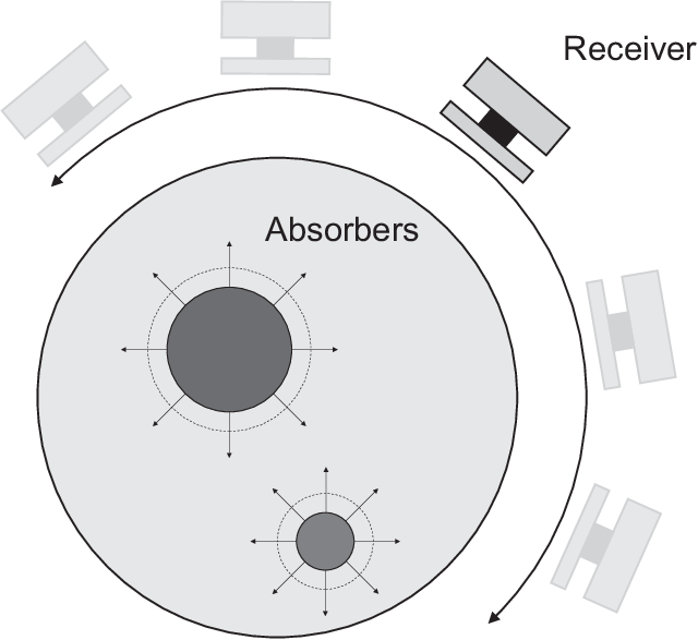
Figure 1: Conventional thermoacoustic scanning system. The non-uniform absorbtion causes outgoing acoustic waves that are measured with an ultrasonic transducer located at different positions.

The measured output of a conventional ultrasonic transducer is the total pressure

$$\frac{1}{|S|}\int_{S}p(\mathbf{x},t)\,dS(\mathbf{x})$$

acting on the surface $S$ of the ultrasonic transducer convolved in time with the temporal impulse response function of the detector [11]. Here $dS$ denotes the two dimensional surface measure and $|S|$ the surface area of $S$. In thermoacoustic CT the temporal impulse response function of the ultrasonic detector is assumed to be an approximation of the $\delta$-distribution and the surface area $|S|$ to be small. In this case the measurement data can be approximated by

$$p(\mathbf{x}_{\rm rec},t)\cong\frac{1}{|S|}\int_{S}p(\mathbf{x},t)\,dS(\mathbf{x})$$

where $\mathbf{x}_{\rm rec}$ is the center of the surface $S$.

In practice conventional piezoelectric ultrasonic transducers placed on a recording surface $S_{\rm rec}$ are used to approximate point-like detectors [15, 25]. In this case thermoacoustic CT leads to the mathematical problem of recovering a function from its integrals over spheres with centers $\mathbf{x}_{\rm rec}$ (locations of the point-like detectors) on $S_{\rm rec}$ [25, 7, 14]. Every ultrasonic transducers has a finite size (typically in the range of mm) and therefore algorithms that are based on the assumption that point measurement data is collected give blurred reconstructions.

Line detectors measure the total pressure

$$\int_{L}p(\mathbf{x},t)\,dL(\mathbf{x})$$

on a line $L$ [5, 19]. In practical experiments they can be realized by a thin laser beam that is either part of Fabry–Perot [5] or Mach–Zehnder [19] interferometer. Details on the technical realization of line detectors can be found in [5, 19]. We just note here that optical sensors offer high bandwidth and high signal to noise ratio.

Data acquisition

Throughout this paper we assume that the initial data $f$ is supported in the open set $V_{\rm rec}$. We call $V_{\rm rec}$ recording volume, if $V_{\rm rec}$ is invariant with respect to rotations around the $\mathbf{e}_{3}=(0,0,1)$ axis, i.e.

$$V_{\rm rec}=\{R\mathbf{x}:\mathbf{x}\in V_{\rm rec}\}$$

holds for all rotations $R\in{\rm SO(3)}$ with fix point set $\mathbb{R}\mathbf{e}_{3}$. Important examples for recording volumes are the half space $\mathbb{R}^{2}\times(0,\infty)$, the cylinder $D\times\mathbb{R}$, where $D$ denotes the unit disc in $\mathbb{R}^{2}$. We set $D_{\rm rec}:=V_{\rm rec}\cap(\{0\}\times\mathbb{R}^{2})$.

The measured data is collected with an array of parallel line detectors that are tangential to $V_{\rm rec}$, orthogonal to $\mathbf{e}_{3}$ and rotated around the axis $\mathbf{e}_{3}$. The rotation $R_{\boldsymbol{\sigma}}$ around the axis $\mathbf{e}_{3}$ is parameterized by $\boldsymbol{\sigma}\in S^{1}$ and defined by

$$R_{\boldsymbol{\sigma}}\mathbf{e}_{1} =\mathbf{e}_{1}(\boldsymbol{\sigma}):=(\sigma_{1},\sigma_{2},0)\,,$$

$$R_{\boldsymbol{\sigma}}\mathbf{e}_{2} =\mathbf{e}_{2}(\boldsymbol{\sigma}):=(-\sigma_{2},\sigma_{1},0)\,,$$

$$R_{\boldsymbol{\sigma}}\mathbf{e}_{3} =\mathbf{e}_{3}\;.$$

Here $(\mathbf{e}_{1},\mathbf{e}_{2},\mathbf{e}_{3})$ denotes the standard basis of $\mathbb{R}^{3}$ and $(\mathbf{e}_{1}(\boldsymbol{\sigma}),\mathbf{e}_{2}(\boldsymbol{\sigma}),\mathbf{e}_{3})$ is a positively oriented orthonormal basis. In practical applications the measurements, for fixed $\boldsymbol{\sigma}$, are performed either with a array or by moving a single line detector along a recording curve $\mathcal{C}_{\rm rec}$.

Let

$$L(\boldsymbol{\sigma},\mathbf{y}):=\{s\mathbf{e}_{1}(\boldsymbol{\sigma})+y_{1}\mathbf{e}_{2}(\boldsymbol{\sigma})+y_{2}\mathbf{e}_{3}:s\in\mathbb{R}\}$$

be a line, where $\mathbf{y}=(y_{1},y_{2})\in\mathbb{R}^{2}$. The positions of the line detectors are given by $L(\boldsymbol{\sigma},\mathbf{y}_{\rm rec})$ with $\mathbf{y}_{\rm rec}\in\mathcal{C}_{\rm rec}\subset\partial D_{\rm rec}$ which is called recording curve, see Figure 2.

Since $V_{\rm rec}$ is rotationally invariant with respect to $\mathbf{e}_{3}$ and $\mathcal{C}_{\rm rec}\subset\partial D_{\rm rec}$ all lines $L(\boldsymbol{\sigma},\mathbf{y}_{\rm rec})$ (locations of the line detectors) are outside the support of $f$. The forward operator

$$\Po:C_{0}^{\infty}(V_{\rm rec}) \to C^{\infty}\left(S^{1}\times\mathcal{C}_{\rm rec}\times(0,\infty)\right)$$

$$f \mapsto\Po(f):=\left((\boldsymbol{\sigma},\mathbf{y}_{\rm rec},t)\mapsto\int_{L(\boldsymbol{\sigma},\mathbf{y}_{\rm rec})}p(\mathbf{x},t)\,dL(\mathbf{x})\right)$$

collects the data measured by all line detectors $L(\boldsymbol{\sigma},\mathbf{y}_{\rm rec})$ for given initial data $f$. Here $p(\mathbf{x},t)$ denotes the unique solution of (1), (2), (3). We note that (1), (2), (3) is a well posed problem and therefore $\Po(f)$ can be calculated stable for arbitrary initial data $f$. Thermoacoustic CT with line detectors deals with the solution of the operator equation $\Po(f)=g$ with given (potentially noisy) measured data $g$. Therefore we study uniqueness, stability and explicit inversion of $\Po$. In this paper we focus on the derivation and implementation of inversion formulas.

Figure 2: Scanning geometry for thermoacoustic CT using line detectors. The line detectors (orthogonal to the drawing plane) are uniformly distributed on the recording curve $\mathcal{C}_{\rm rec}$ and rotated around a single axis of rotation $\mathbf{e}_{3}$, indicated by parameter $\boldsymbol{\sigma}$.

3 Decomposition of the three dimensional forward operator into a system of two dimensional operators

Let $V_{\rm rec}$ be a recording volume and $\mathcal{C}_{\rm rec}\subset\partial D_{\rm rec}$ a recording curve. In this Section we prove that the corresponding forward operator $\Po$ decomposes into the product of the two dimensional Radon transform $\Ro$ and the operator

$$\Qo:C_{0}^{\infty}(D_{\rm rec}) \to C^{\infty}\big(\mathcal{C}_{\rm rec}\times(0,\infty)\big)$$

$$F \mapsto\Qo(F):=\big((\mathbf{y}_{\rm rec},t)\mapsto P(\mathbf{y}_{\rm rec},t)\big)$$

that maps a planar function $F\in C_{0}^{\infty}(D_{\rm rec})$ onto the solution $P$ of the two dimensional wave equation

$$\left(\frac{\partial^{2}}{\partial t^{2}}-\Delta_{\mathbf{y}}\right)P=0\,,\qquad(\mathbf{y},t)\in\mathbb{R}^{2}\times(0,\infty)$$ (4)

with initial conditions

$$P(\mathbf{y},0)=F(\mathbf{y})\,, \mathbf{y}\in\mathbb{R}^{2}\,,$$ (5)

$$\frac{\partial P}{\partial t}(\mathbf{y},0)=0\,, \mathbf{y}\in\mathbb{R}^{2}$$ (6)

restricted to the recording curve $\mathcal{C}_{\rm rec}$. Here $\Delta_{\mathbf{y}}$ denotes the Laplacian in $\mathbb{R}^{2}$. We use the following notation:

1. Define

   $$\Ro\otimes\Io_{3}:C_{0}^{\infty}(V_{\rm rec}) \to C_{0}^{\infty}(S^{1}\times\mathbb{R}^{2})$$

   $$f \mapsto(\Ro\otimes\Io_{3})(f):=\Big(\big(\boldsymbol{\tau},(r,z)\big)\mapsto\big({\cal R}(f_{z})\big)(\boldsymbol{\tau},r)\Big)$$

   where $\Ro$ denotes the classical two dimensional Radon transform [17] defined by

   $$\Ro:C_{0}^{\infty}(\mathbb{R}^{2}) \to C_{0}^{\infty}(S^{1}\times\mathbb{R})$$

   $$\varphi \mapsto\Ro(\varphi):=\left((\boldsymbol{\tau},r)\mapsto\int_{\mathbb{R}}\varphi(s\boldsymbol{\tau}+r\boldsymbol{\tau}^{\perp})\,ds\right)$$

   and $f_{z}$ the function $f$ for fixed third parameter $z$, i.e.

   $$f_{z}(x,y):=f(x,y,z)\,,\quad\textrm{with $z\in\mathbb{R}$ fixed\;.}$$

   Here $\boldsymbol{\tau}^{\bot}$ is a unit vector orthogonal to $\boldsymbol{\tau}$. The notation indicates that the operator $\Ro\otimes\Io_{3}$ operates on a function $f$ defined on $\mathbb{R}^{3}$ by applying the Radon transform to the first two components for fixed third component.

2. For a fixed $\boldsymbol{\tau}\in S^{1}$ and a function $G\in C_{0}^{\infty}(S^{1}\times D_{\rm rec})$ define

   $$G_{\boldsymbol{\tau}}(x_{1},x_{2}):=G(\boldsymbol{\tau},x_{1},x_{2})\;.$$

   Furthermore, we define an operator $\Io\otimes\Qo$ by

   $$\Io\otimes\Qo:C_{0}^{\infty}(S^{1}\times D_{\rm rec}) \to C^{\infty}\big(S^{1}\times\mathcal{C}_{\rm rec}\times(0,\infty)\big)$$

   $$G \mapsto(\Io\otimes\Qo)(G):=\big((\boldsymbol{\tau},\mathbf{y}_{\rm rec},t)\mapsto\big(\Qo(G_{\boldsymbol{\tau}})\big)(\mathbf{y}_{\rm rec},t)\big)\;.$$

The main feature of using line detectors is based on the following decomposition:

Theorem 1.

Let $f\in C_{0}^{\infty}(V_{\rm rec})$. Then

$$\Po(f)=(\Io\otimes\Qo)\circ(\Ro\otimes\Io_{3})(f)\;.$$ (7)

Proof.

Let $f\in C^{\infty}_{0}(V_{\rm rec})$, $p$ be the solution of (1), (2), (3) and fix $\boldsymbol{\sigma}\in S^{1}$. We define

$$P(\mathbf{y},t):=\int_{L(\boldsymbol{\sigma},\mathbf{y})}p(\mathbf{x},t)\,dL(\mathbf{x})$$

and show that $P$ is the unique solution of the two dimensional wave equation (4), (5), (6) with initial data $F=(\Ro\otimes\Io_{3})(f)(\boldsymbol{\sigma},\cdot)$. Theorem 1 then follows from the fact that $\Po(f)(\boldsymbol{\sigma},\mathbf{y}_{\rm rec},t)=P(\mathbf{y}_{\rm rec},t)$ for $\mathbf{y}_{\rm rec}\in\mathcal{C}_{\rm rec}$ and $t\geq 0$. From (2), (3) and the definitions of $(\Ro\otimes\Io_{3})(f)$ and $P$ it follows immediately that $P$ satisfies the initial conditions (5), (6). It remains to prove that $P$ satisfies (4).

Since $(\mathbf{e}_{1}(\boldsymbol{\sigma}),\mathbf{e}_{2}(\boldsymbol{\sigma}),\mathbf{e}_{3})$ is an orthonormal basis of $\mathbb{R}^{3}$ for every $\mathbf{x}\in\mathbb{R}^{3}$ there exist unique elements $s\in\mathbb{R}$ and $\mathbf{y}\in\mathbb{R}^{2}$ such that $\mathbf{x}=s\mathbf{e}_{1}(\boldsymbol{\sigma})+\mathbf{y}=:s\mathbf{e}_{1}(\boldsymbol{\sigma})+y_{1}\mathbf{e}_{2}(\boldsymbol{\sigma})+y_{2}\mathbf{e}_{3}$. Therefore, the Laplacian in $\mathbb{R}^{3}$ decomposes into the sum

$$\Delta_{\mathbf{x}}=\frac{\partial^{2}}{\partial s^{2}}+\Delta_{\mathbf{y}}\;.$$

Using (1) results in

$$0 =\int_{\mathbb{R}}\left(\frac{\partial^{2}p}{\partial t^{2}}(s\mathbf{e}_{1}(\boldsymbol{\sigma})+\mathbf{y},t)-\frac{\partial^{2}p}{\partial s^{2}}(s\mathbf{e}_{1}(\boldsymbol{\sigma})+\mathbf{y},t)-\Delta_{\mathbf{y}}p(s\mathbf{e}_{1}(\boldsymbol{\sigma})+\mathbf{y},t)\right)ds$$

$$=\frac{\partial^{2}}{\partial t^{2}}\int_{\mathbb{R}}p(s\mathbf{e}_{1}(\boldsymbol{\sigma})+\mathbf{y},t)\,ds-\left[\frac{\partial p}{\partial s}(s\mathbf{e}_{1}(\boldsymbol{\sigma})+\mathbf{y},t)\right]_{s=-\infty}^{s=\infty}$$

$$-\Delta_{\mathbf{y}}\int_{\mathbb{R}}p(s\mathbf{e}_{1}(\boldsymbol{\sigma})+\mathbf{y},t)\,ds$$

$$=\frac{\partial^{2}P}{\partial t^{2}}(\mathbf{y},t)-\Delta_{\mathbf{y}}P(\mathbf{y},t)\;.$$

The last equality holds since $p(\cdot,t)$ is compactly supported [12] for all $t\geq 0$. Hence $P$ satisfies (4). ∎

The decomposition of $\Po$ into a set of lower dimensional operators can be used to reduces the complexity of the derived reconstruction algorithms.

The operator $\Qo$ is closely related to the circular Radon transform with center set $\mathcal{C}_{\rm rec}$ [7, 18], which is defined by

$$\Mo:C_{0}^{\infty}(D_{\rm rec}) \to C^{\infty}\big(\mathcal{C}_{\rm rec}\times(0,\infty)\big)$$

$$F \mapsto\Mo(F):=\left((\mathbf{y}_{\rm rec},r)\mapsto\frac{1}{2\pi}\int_{S^{1}}F(\mathbf{y}_{\rm rec}+r\boldsymbol{\omega})\,d\Omega(\boldsymbol{\omega})\right)$$

and maps a function $F\in C_{0}^{\infty}(D_{\rm rec})$ onto its integrals over circles with centers on the recording curve $\mathcal{C}_{\rm rec}$.

Using D’Alembert’s formula the solution of (4), (5), (6) turns out to be [12]

$$\big(\Qo(F)\big)(\mathbf{y}_{\rm rec},t)=\frac{\partial}{\partial t}\int_{0}^{t}\frac{r\Mo(F)(\mathbf{y}_{\rm rec},r)}{\sqrt{t^{2}-r^{2}}}\,dr$$ (8)

which means that $\Qo(F)$ can be calculated if the circular Radon transform $\Mo(F)$ of $F$ is known. The following Lemma states that also the reversal is true:

Lemma 1.

Let $F\in C_{0}^{\infty}(D_{\rm rec})$. Then

$$\Mo(F)(\mathbf{y}_{\rm rec},r)=\frac{2}{\pi}\int_{0}^{r}\frac{\Qo(F)(\mathbf{y}_{\rm rec},t)}{\sqrt{r^{2}-t^{2}}}\;dt$$ (9)

for all $\mathbf{y}_{\rm rec}\in\mathcal{C}_{\rm rec}$ and $t\geq 0$.

A proof of a generalization of Lemma 1 is given in [23, Theorem 2.1.2], but for the sake of completeness we prove Lemma 1 since it is an elementary proof.

Proof.

Let $F\in C_{0}^{\infty}(D_{\rm rec})$, fix $\mathbf{y}_{\rm rec}\in\mathcal{C}_{\rm rec}$ and define $\Phi(t):=\Mo(F)(\mathbf{y}_{\rm rec},t)$. Furthermore, we define for a function $\Psi\in C^{\infty}\big((0,\infty)\big)$

$$\big(\Jo(\Psi)\big)(u) :=\int_{0}^{u}\frac{\Psi(t)}{\sqrt{u^{2}-t^{2}}}\;dt\,,$$

$$\big(\Jo_{\rm mul}(\Psi)\big)(u) :=\int_{0}^{u}t\frac{\Psi(t)}{\sqrt{u^{2}-t^{2}}}\;dt\,,$$

$$\big(\Ko(\Psi)\big)(u) :=u\big(\Jo(\Psi)\big)(u)\;.$$

Due to equation (8) it is sufficient to prove that $(2/\pi)\Jo\big(\big(\Jo_{\rm mul}(\Phi)\big)^{\prime}\big)=\Phi$. As an auxiliary result we prove that for all $\Psi\in C^{\infty}((0,\infty))$

$$I(r):=\big(\Jo\big(\Ko(\Psi)\big)\big)(r)=\frac{\pi}{2}\int_{0}^{r}\Psi(u)du\;.$$ (10)

For the proof of (10) let $t>0$ and consider the integral

$$I(r)=\int_{0}^{r}\frac{t\Jo(\Psi)(t)}{\sqrt{r^{2}-t^{2}}}\;dt=\int_{0}^{r}\left(\int_{0}^{t}\Psi(u)\frac{du}{\sqrt{t^{2}-u^{2}}}\right)\frac{t}{\sqrt{r^{2}-t^{2}}}\;dt\;.$$

From Fubini’s theorem we conclude that

$$I(r)=\int_{0}^{r}\left(\int_{u}^{r}\frac{t}{\sqrt{t^{2}-u^{2}}\sqrt{r^{2}-t^{2}}}\;dt\right)\Psi(u)du$$

We substitute $t=\sqrt{u^{2}+v^{2}}$ and $dt=(v/t)dv$ in the inner integral. Therefore

$$I(r)=\int_{0}^{r}\left(\int_{0}^{\sqrt{r^{2}-u^{2}}}\frac{dv}{\sqrt{r^{2}-u^{2}-v^{2}}}\right)\Psi(u)du\;.$$

Finally, we use the substitution $v=\sqrt{r^{2}-u^{2}}\sin(\alpha)$ and $dv=\sqrt{r^{2}-u^{2}}\cos(\alpha)d\alpha$. We obtain

$$I(r)=\int_{0}^{r}\left(\int_{0}^{\pi/2}d\alpha\right)\Psi(u)du=\frac{\pi}{2}\int_{0}^{r}\Psi(u)du\;.$$

Hence we have proved (10).

Next we prove that

$$\big(\Jo_{\rm mul}(\Phi)\big)^{\prime}=\Ko(\Phi^{\prime})\;.$$ (11)

Using the relation

$$\frac{\partial}{\partial r}\sqrt{t^{2}-r^{2}}=-\frac{r}{\sqrt{t^{2}-r^{2}}}$$

and integration by parts we obtain

$$\int_{0}^{t}\frac{r\Phi(r)}{\sqrt{t^{2}-r^{2}}}dr =\left[\Phi(r)\sqrt{t^{2}-r^{2}}\right]_{r=0}^{r=t}+\int_{0}^{t}\Phi^{\prime}(r){\sqrt{t^{2}-r^{2}}}dr$$

$$=\int_{0}^{t}\Phi^{\prime}(r){\sqrt{t^{2}-r^{2}}}dr\;.$$

By differentiating the above equation with respect to $t$ we obtain

$$\left(\int_{0}^{t}\frac{r\Phi(r)}{\sqrt{t^{2}-r^{2}}}dr\right)^{\prime}(t) =\left[\Phi^{\prime}(r)\sqrt{t^{2}-r^{2}}\right]_{r=t}+t\int_{0}^{t}\frac{\Phi^{\prime}(r)}{\sqrt{t^{2}-r^{2}}}\,dr\;.$$

$$=\big(\Ko(\Phi^{\prime})\big)(t)$$

Hence we have proved (11). Applying $\Jo$ to (11) we find

$$\Jo\big(\big(\Jo_{\rm mul}(\Phi)\big)^{\prime}\big)=\Jo\big(\Ko(\Phi^{\prime})\big)=\frac{\pi}{2}\Phi\;.$$

For the last equality we applied the auxiliary result (10) to $\Psi=\Phi^{\prime}$. ∎

In order to prove that $\Po$ is injective we use Lemma 1 and a uniqueness result for the circular Radon transform.

Theorem 2 (Uniqueness for arbitrary recording curve).

Let $V_{\rm rec}$, $D_{\rm rec}$ and $\mathcal{C}_{\rm rec}$ be as above, and assume additionally, that $D_{\rm rec}$ is convex and that $\mathcal{C}_{\rm rec}\subset D_{\rm rec}$ is a relatively open $C^{1}$ curve. If $f\in C_{0}^{\infty}(V_{\rm rec})$ and $\Po(f)=0$, then $f=0$.

Proof.

Due to (7) it is sufficient to show that $\Ro$ and $\Qo$ are injective. It is well known that the Radon transform $\Ro$ is injective, see for example [17, Theorem 2]. Therefore, it remains to show that $\Qo$ is injective.

Let $F\in C_{0}^{\infty}(D_{\rm rec})$ and $\Qo(F)=0$. From (9) it follows that $\Mo(F)=0$. It is known that the circular Radon transform with center set $D_{\rm rec}$ is injective, see [2, Theorem 19] (compare also with [1, 7]). We conclude that $F=0$ which means that $\Qo$ is injective. ∎

Equation (7) implies that thermoacoustic CT with line detectors deals with the inversion of the operator $\Qo$ and the inversion of the two dimensional classical Radon transform $\Ro$. Fast and stable algorithms for inverting the two dimensional classical Radon transform $\Ro$ are well investigated. The key task for deriving inversion algorithms for $\Po$ is the inversion of the operator $\Qo$. Therefore, in the next Section we present and analyze an analytic formula for inverting $\Qo$.

4 Linear recording curve: Inversion of the two dimensional wave equation from data on a line

Throughout the remaining parts of this article we consider the case where the recording curve $\mathcal{C}_{\rm rec}\subset\mathbb{R}^{2}$ is a line. Depending on the angle between $\mathcal{C}_{\rm rec}$ and $\mathbf{e}_{2}$, the recording volume $V_{\rm rec}$ is either a closed cylinder, a closed cone or a half space, each considered as a subset of $\mathbb{R}^{3}$ (see Figure 3). In all cases $\Qo$ maps the initial data $F$ onto the solution of of the two dimensional wave equation (4)-(6) restricted to $\mathcal{C}_{\rm rec}$.

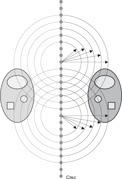
Figure 3: The array of line detectors measures the solution of the two dimensional wave equation (4)-(6) restricted to $\mathcal{C}_{\rm rec}$ and is rotated in a plane (top left), tangential to a cylinder (top right) or tangential to a cone (bottom left). Bottom right: The restriction of the solution to $\mathcal{C}_{\rm rec}$ is uniquely determined by the means over circles with centers on $\mathcal{C}_{\rm rec}$ (see (8)) and remains unchanged after symmetrizing the initial data $F$ around $\mathcal{C}_{\rm rec}$.

From symmetry properties of the wave equation (bottom right image in Figure 3) it follows that in order to invert $\Qo$ it is sufficient to solve the following problem: Recover $H\in C_{0}^{\infty}(\mathbb{R}\times(0,\infty))$ from data $G:=P|_{\mathbb{R}\times\{0\}\times(0,\infty)}$, where $P$ is the solution of

$$\left(\frac{\partial^{2}}{\partial t^{2}}-\frac{\partial^{2}}{\partial u^{2}}-\frac{\partial^{2}}{\partial v^{2}}\right)P=0\,,\quad(u,v,t)\in\mathbb{R}^{2}\times(0,\infty)$$ (12)

with symmetric initial conditions

$$P(u,v,0)=H(u,|v|)\,, (u,v)\in\mathbb{R}^{2}\,,$$ (13)

$$\frac{\partial P}{\partial t}(u,v,0)=0\,, (u,v)\in\mathbb{R}^{2}.$$ (14)

$u$ denotes the coordinate in direction $\mathcal{C}_{\rm rec}$ and $v$ the signed distance to the orthogonal direction.

In the following we have to apply the Fourier–cosine transform to $G$. Since $G\not\in L^{1}(\mathbb{R}\times(0,\infty))$, see Corollary 1 below, we have to sidestep to the space of symmetric tempered distributions. See Appendix A for the definitions of the spaces $S_{\rm sym}(\mathbb{R}\times\mathbb{R})$, $C^{oo}_{\rm sym}(\mathbb{R}\times\mathbb{R})$, $S^{\prime}_{\rm sym}(\mathbb{R}\times\mathbb{R})$, the Fourier–cosine transforms $\cost$, $\costp$ and the natural injections $\injS$, $\injL$, $\injC$ that map functions onto tempered distributions. We note that, since $G_{\rm sym}\in C^{oo}(\mathbb{R}\times\mathbb{R})$, $\injC[G_{\rm sym}]\in S^{\prime}_{\rm sym}(\mathbb{R}\times\mathbb{R})$ and the Fourier–cosine transform $\costp[\injC[G_{\rm sym}]]$ is well defined, see Appendix A for details.

Theorem 3 (Fourier inversion formula).

Let $H\in C_{0}^{\infty}(\mathbb{R}\times(0,\infty))$, $P$ be the solution of (12)-(14), $G:=P|_{\mathbb{R}\times\{0\}\times(0,\infty)}$ and $\Omega:=\{(\omega,\lambda)\in\mathbb{R}^{2}:\omega>|\lambda|\}$. Then there exists $\bar{G}\in L^{1}(\mathbb{R}\times(0,\infty))\cap C^{\infty}(\Omega)$ with $\costp[\injC[G_{\rm sym}]]=\injL[\bar{G}_{\rm sym}]$, and the Fourier inversion formula holds

$$\cost[H](\lambda,\kappa)=\bar{G}\left(\lambda,\sqrt{\kappa^{2}+\lambda^{2}}\right)\cdot\displaystyle\frac{\kappa}{\sqrt{\kappa^{2}+\lambda^{2}}}$$ (15)

point–wise for all $(\lambda,\kappa)\in\mathbb{R}\times(0,\infty)$.

Proof.

An elementary calculation shows that for all $(\lambda,\kappa)\in\mathbb{R}\times(0,\infty)$ the functions

$$\cos(\kappa v)e^{i\lambda u}\cos\left(t\sqrt{\kappa^{2}+\lambda^{2}}\right)$$

are solutions of (12) and (14). Since $H\in C_{0}^{\infty}(\mathbb{R}\times(0,\infty))\subset S_{\rm sym}(\mathbb{R}\times\mathbb{R})$, $\bar{H}:=\cost[H]$ is well defined. From the linearity of the wave equation and the inversion formula for the Fourier–cosine transform on $S_{\rm sym}(\mathbb{R}\times\mathbb{R})$, see Proposition 3 in Appendix A, it follows that the unique solution of (12)-(14) is given by

$$P(u,v,t)=\frac{1}{\pi}\int_{\mathbb{R}}\left(\int_{0}^{\infty}\bar{H}(\lambda,\kappa)\cos\left(t\sqrt{\kappa^{2}+\lambda^{2}}\right)\cos(\kappa v)\,d\kappa\right)e^{i\lambda u}d\lambda\;.$$

Substituting $\kappa^{2}=\omega^{2}-\lambda^{2}$ in the inner integral and taking $v=0$ leads to

$$G(u,t)=\frac{1}{\pi}\int_{\mathbb{R}}\left(\int_{|\lambda|}^{\infty}\bar{H}\left(\sqrt{\omega^{2}-\lambda^{2}},\lambda\right)\cos(\omega t)\frac{\omega d\omega}{\sqrt{\omega^{2}-\lambda^{2}}}\right)e^{i\lambda u}d\lambda\;$$ (16)

Define a function $\bar{G}$ by

$$\bar{G}(\lambda,\omega):=\begin{cases}\bar{H}(\lambda,\sqrt{\omega^{2}-\lambda^{2}})\omega/\sqrt{\omega^{2}-\lambda^{2}}&\textrm{if }\omega>|\lambda|\\ 0&\textrm{otherwise}\;.\end{cases}$$ (17)

$\bar{G}$ satisfies

$$\|\bar{G}\|_{L^{1}}=\int_{R}\int_{0}^{\infty}|\bar{G}(\lambda,\omega)|\,d\omega\,d\lambda=\int_{R}\left(\int_{k}^{\infty}|\bar{H}\left(\lambda,\sqrt{\omega^{2}-\lambda^{2}}\right)|\frac{\omega d\omega}{\sqrt{\omega^{2}-\lambda^{2}}}\right)d\lambda\;.$$

Substituting $\omega^{2}=\kappa^{2}+\lambda^{2}$ in the inner integral we conclude that $\|\bar{G}\|_{L^{1}}=\|\bar{H}\|_{L^{1}}$ and hence $\bar{G}\in L^{1}(\mathbb{R}\times(0,\infty))$. Equation (16) and $\bar{G}\in L^{1}(\mathbb{R}\times(0,\infty))$ imply that $\cost[\bar{G}]^{-}=G$ and since the definitions of the Fourier–cosine transforms on $S^{\prime}_{\rm sym}(\mathbb{R}\times\mathbb{R})$ and $L^{1}(\mathbb{R}\times(0,\infty))$ are compatible, see Proposition 2

$$\icostp[\injL[\bar{G}_{\rm sym}]]=\injC[\cost[\bar{G}]_{\rm sym}^{-}]=\injC[G_{\rm sym}]\;.$$

Applying the inversion formula for the Fourier–cosine transform on $S^{\prime}_{\rm sym}(\mathbb{R}\times\mathbb{R})$, see Proposition 1, shows $\injL[\bar{G}_{\rm sym}]=\costp[\injC[G_{\rm sym}]]$.

Finally, solving (17) for $\bar{H}$ shows that (15) holds point–wise for all $\kappa=\sqrt{\omega^{2}-\lambda^{2}}>0$. ∎

Corollary 1.

Let $H$, $G$ and $\bar{G}$ be as in Theorem 3. Moreover, assume that $H\neq 0$ is non–negative. Then $G$ is not absolutely integrable.

Proof.

Assuming $G\in L^{1}(\mathbb{R}\times(0,\infty))$ it follows from Proposition 3 in Appendix A that $\bar{G}=\cost[G]\in C^{oo}(\mathbb{R}\times(0,\infty))$. Since $H$ is non–vanishing it follows that $\cost[H](0,0)>0$ and since $\cost[H]$ is continuous there exists $\varepsilon>0$, such that $\cost[H](\varepsilon,\varepsilon)>0$. Inserting the sequence $(\varepsilon+1/n,\varepsilon+2/n)$ in (17) shows that $\bar{G}$ is unbounded, contradicting $\bar{G}\in C^{oo}(\mathbb{R}\times(0,\infty))$. ∎

Corollary 1 implies that the integral

$$\frac{1}{\pi}\int_{\mathbb{R}}\int_{0}^{\infty}G(u,t)\cos(\omega t)e^{-i\lambda u}dt\,du$$ (18)

is not absolutely convergent and therefore cannot be used directly to find an analytic representation of $\bar{G}$. However, in the following we show that (18) exists in some generalized sense and can be used to find an analytic representation of $\bar{G}$.

In the following

$$\ft_{1}[\Phi](\lambda) :=\left(\frac{1}{2\pi}\right)^{1/2}\int_{\mathbb{R}}\Phi(u)e^{-i\lambda u}du\,,\quad\lambda\in\mathbb{R}\,,$$

$$\cost_{2}[\Phi](\omega) :=\left(\frac{2}{\pi}\right)^{1/2}\int_{0}^{\infty}\Phi(t)\cos(\omega t)dt\,,\quad\omega>0$$

denote the one dimensional Fourier transform on $L^{1}(\mathbb{R})$ and the Fourier-cosine transform on $L^{1}((0,\infty))$, respectively. When applied to a function defined on $\mathbb{R}\times(0,\infty)$ $\ft_{1}$ acts on the first and $\cost_{2}$ on the second component. Finally, we recall the following special case of Jordan’s theorem: If $\Phi\in L^{1}((0,\infty))$ is continuous differentiable on an interval including the point $\omega>0$, then

$$\Phi(\omega)=\lim_{K\to\infty}\left(\frac{2}{\pi}\right)^{1/2}\int_{0}^{K}\cos(\omega t)\cost_{2}[\Phi](t)\,dt\;.$$ (19)

This enables us to prove our final result, namely an explicit expression for the calculation of $\bar{G}$.

Theorem 4 (Analytic formula for $\bar{G}$).

Let $H$, $G$, $\bar{G}$ and $\Omega$ as in Theorem 3. Then, for $(\lambda,\omega)\in\Omega$

$$\bar{G}(\lambda,\omega)=\lim_{K\to\infty}\frac{1}{\pi}\int_{0}^{K}\left(\int_{\mathbb{R}}G(u,t)e^{-i\lambda u}du\right)\cos(\omega t)\,dt\;.$$ (20)

Proof.

From Theorem 3 it follows that $\bar{G}\in L^{1}(\mathbb{R}\times(0,\infty))$ and $\cost[\bar{G}]=G^{-}$. Fubini’s theorem implies that

$$\ft_{1}\circ\cost_{2}[\bar{G}]=\cost[\bar{G}]=G^{-}.$$ (21)

Since the initial data $H$ of the two dimensional wave equation (12)-(14) is compactly supported, $G(\cdot,t)\in C_{0}^{\infty}(\mathbb{R})$ for fixed $t\geq 0$ and therefore $\ft_{1}[G](\cdot,t)\in S(\mathbb{R})$. Hence, applying $\ft_{1}$ to (21) yields

$$\ft_{1}[G]^{-}=\cost_{2}[\bar{G}]^{-}$$ (22)

Next we apply (19) to $\bar{G}(\lambda,\cdot)$, for fixed $\lambda$,

$$\bar{G}(\lambda,\omega)=\lim_{K\to\infty}\left(\frac{2}{\pi}\right)^{1/2}\int_{0}^{K}\cost_{2}[\bar{G}](\lambda,t)\cos(\omega t)\,dt\;.$$ (23)

In order to finish the proof we apply (22) to the integrand of (23) and obtain

$$\bar{G}(\lambda,\omega) = \lim_{K\to\infty}\left(\frac{2}{\pi}\right)^{1/2}\int_{0}^{K}\ft_{1}[G](\lambda,t)\cos(\omega t)\,dt$$

$$= \lim_{K\to\infty}\frac{1}{\pi}\int_{0}^{K}\left(\int_{\mathbb{R}}G(u,t)e^{-i\lambda u}du\right)\cos(\omega t)\,dt\;.$$

∎

Theorem 4 shows that the calculation of the Fourier–cosine transform in the space $S^{\prime}_{\rm sym}(\mathbb{R}\times\mathbb{R})$ of tempered distributions can be avoided. Moreover, in practical applications data $G(u,t)$ can be collected on a finite space-time domain only. The fact that $G(\cdot,t)$ is compactly supported for $t$ fixed and Theorem 4 justify that, in order to approximately calculate $\bar{G}$, the domain of integration in (20) can be replaced by this finite domain. However, data truncation will introduce error in the reconstruction.

Figure 4: Reconstruction with Fourier Formula. Top left. Initial data $H$. Top right. Simulated data with $|u|\leq 100$ mm. Bottom left. Reconstruction from exact data. Bottom right. Reconstruction from noisy data.

Remark 1 (Numerical realization).

It is straight forward to derive a fast Fourier reconstruction algorithm based on Theorems 3, 4: First use the FFT algorithm to approximate $\bar{G}$, see (20). Then use bilinear interpolation and (15) to approximate $\cost[F]$ on a cartesian grid. Finally, again by using the FFT algorithm, calculate an approximation of $F$. Due to the FFT algorithm, using data $G$ to calculate $F$ at ${\tt N^{2}}$ grid points, the numerical effort is $O({\tt N^{2}}\log{\tt N})$ only.

Figure 4 shows results of a numerical example with initial data consisting of nine spheres supported in $[-10,10]\times[0,20]$. Data was collected with an array covering $[-100,100]$. The solution of (12)-(14) was calculated analytically and uniformly distributed random noise with values in the interval $[-e,e]$, where $e$ equals to $5\%$ of the largest data value, was added. The bottom images are obtained via the Fourier reconstruction formula, as presented in the Remark 1.

The left image in Figure 5 shows a reconstruction where data was collected for $u\in[-20,20]$ only (limited aperture). In this case, boundaries of some spheres are not recovered correctly. We emphasize that this confirms theoretical predictions from microlocal analysis [16], namely that in order to stable recover a boundary with tangent $\mathbf{t}$ at $P_{i}=(u_{i},v_{i})$, data $G(u,\cdot)$ has to be collected such that $(u_{i}-u,v_{i})$ is orthogonal to $\mathbf{t}$. As illustrated in Figure 5, this requirement is not satisfied for nearly horizontal boundaries.

Figure 5: Finite aperture effect. Left. Reconstruction from data $P(u,t)$ with $|u|\leq 20$ mm. Nearly horizontal boundaries are not recovered correctly. Right. The boundary $(P_{1},\mathbf{t}_{1})$ can be recovered stable, the boundary $(P_{2},\mathbf{t}_{2})$ cannot.

5 Conclusion and outlook

In this paper we presented a mathematical framework of thermoacoustic CT with line detectors. The advantage of using line detectors is the improved imaging resolution compared to data acquisition based on point data. We proved that the three dimensional imaging problem reduces to the problem of reconstructing the initial data of the two dimensional wave equation from boundary measurements.

In practical applications the output of a planar detector array offers only information from a finite aperture. Therefore, our future work will focus on the case of limited data. Furthermore, we will investigate scanning geometries where the array of line detectors forms different surfaces, e.g. cylinders which allow to collect a complete data set.

Appendix A The Fourier–cosine transform on the space of symmetric tempered distributions

In this appendix we define the Fourier–cosine transform on the space of symmetric tempered distributions and prove the propositions stated in Section 4. We will reduce the Fourier–cosine to the Fourier transform and therefore recall the basic definitions and properties of tempered distributions and the Fourier transform [21].

The Schwartz space $S(\mathbb{R}^{n}\times\mathbb{R})$ denotes the set of all infinitely differentiable functions $\varphi:\mathbb{R}^{n}\times\mathbb{R}\to\mathbb{C}$ that are rapidly decreasing together with all their derivatives, i.e.

$$\forall m\in\mathbb{N}_{0},\boldsymbol{\beta}\in\mathbb{N}_{0}^{n+1}:\|\varphi\|_{m,\boldsymbol{\beta}}:=\sup_{\mathbf{u}^{\prime}\in\mathbb{R}^{n+1}}(1+\|\mathbf{u}^{\prime}\|^{m})|D^{\boldsymbol{\beta}}\varphi(\mathbf{u}^{\prime})|<\infty$$

The variables in $\mathbb{R}^{n}\times\mathbb{R}$ are denoted by $\mathbf{u}^{\prime}=(\mathbf{u},v)$. We discriminate between $\mathbf{u}$ and $v$ since the last component will play a special role. Equipped with the topology generated by the semi-norms $\|\varphi\|_{m,\boldsymbol{\beta}}$, where $m\in\mathbb{N}_{0}$, $\boldsymbol{\beta}\in\mathbb{N}_{0}^{n+1}$, $S(\mathbb{R}^{n}\times\mathbb{R})$ is a Fréchet space (metrizable and locally convex).

The space $S^{\prime}(\mathbb{R}^{n}\times\mathbb{R})$ of tempered distributions is defined as the topological dual of $S$, i.e. the set of all linear continuous functionals $T:S(\mathbb{R}^{n}\times\mathbb{R})\to\mathbb{C}$, equipped with the weak–${}\ast$ topology $\sigma(S^{\prime}(\mathbb{R}^{n}\times\mathbb{R}),S(\mathbb{R}^{n}\times\mathbb{R}))$. The evaluation of a tempered distribution is denoted by $\langle T,\varphi\rangle:=T(\varphi)$. The mappings $\injS:S(\mathbb{R}^{n}\times\mathbb{R})\to S^{\prime}(\mathbb{R}^{n}\times\mathbb{R})$, $\injL:L^{1}(\mathbb{R}^{n}\times\mathbb{R})\to S^{\prime}(\mathbb{R}^{n}\times\mathbb{R})$, and $\injC:C^{oo}(\mathbb{R}^{n}\times\mathbb{R})\to S^{\prime}(\mathbb{R}^{n}\times\mathbb{R})$, where $C^{oo}(\mathbb{R}^{n}\times\mathbb{R})$ denotes the set of all continuous functions $\varphi$ with $\lim_{\|\mathbf{u}^{\prime}\|\rightarrow\infty}\varphi(\mathbf{u}^{\prime})=0$ are well defined and injective. In all cases a function $\varphi$ is mapped to the distribution $\inj[\varphi]$ defined by

$$\langle\inj[\varphi],\psi\rangle:=\int_{\mathbb{R}^{n+1}}\varphi(\mathbf{u}^{\prime})\psi(\mathbf{u}^{\prime})d^{n+1}\mathbf{u}^{\prime}\,,$$

where $\inj$ stands either for $\injS$, $\injL$ or $\injC$.

Definition 1.

• For $\varphi:\mathbb{R}^{n}\times(0,\infty)\to\mathbb{C}$ and $\psi:\mathbb{R}^{n}\times\mathbb{R}\to\mathbb{C}$ define

  $$\varphi_{\rm sym}:\mathbb{R}^{n}\times\mathbb{R} \to\mathbb{C}$$

  $$(\mathbf{u},v) \mapsto\varphi_{\rm sym}(\mathbf{u},v):=\varphi(\mathbf{u},|v|)\,,$$

  $$\psi_{-}:\mathbb{R}^{n}\times\mathbb{R} \to\mathbb{C}$$

  $$(\mathbf{u},v) \mapsto\psi_{-}(\mathbf{u},v):=\psi(\mathbf{u},-v)\,,$$

  $$\psi^{-}:\mathbb{R}^{n}\times\mathbb{R} \to\mathbb{C}$$

  $$(\mathbf{u},v) \mapsto\psi^{-}(\mathbf{u},v):=\psi(-\mathbf{u},v)\,,$$

  $$\psi_{-}^{-}:\mathbb{R}^{n}\times\mathbb{R} \to\mathbb{C}$$

  $$(\mathbf{u},v) \mapsto\psi_{-}^{-}(\mathbf{u},v):=\psi(-\mathbf{u},-v)\;.$$

• The Fourier transform on $L^{1}(\mathbb{R}^{n}\times\mathbb{R})$ is defined by

  $$F:L^{1}(\mathbb{R}^{n}\times\mathbb{R})\rightarrow C^{oo}(\mathbb{R}^{n}\times\mathbb{R})$$

  $$\varphi\mapsto\ft[\varphi]:=\bigg((\boldsymbol{\lambda},\kappa)\mapsto\left(\frac{1}{2\pi}\right)^{(n+1)/2}\int_{\mathbb{R}^{n}}\left(\int_{\mathbb{R}}\varphi(\mathbf{u},v)e^{-i\kappa v}dv\right)e^{-i\langle\boldsymbol{\lambda},\mathbf{u}\rangle}d^{n}\mathbf{u}\bigg)\;.$$

• The Fourier transform $\ft:S(\mathbb{R}^{n}\times\mathbb{R})\to S(\mathbb{R}^{n}\times\mathbb{R})$ restricted to the Schwartz space is well defined and a topological isomorphism (linear, bijective and bicontinuous) with inverse $\ift[\Phi]=\ft[\Phi]_{-}^{-}$.

• The Fourier transform on $S^{\prime}(\mathbb{R}^{n}\times\mathbb{R})$

  $$\ftp:S^{\prime}(\mathbb{R}^{n}\times\mathbb{R}) \rightarrow S^{\prime}(\mathbb{R}^{n}\times\mathbb{R})$$

  $$T \mapsto\ftp[T]:=\big(\varphi\mapsto\langle T,\ft[\varphi]\rangle\big)$$

  is a topological isomorphism with $\langle\iftp[T],\varphi\rangle=\langle T,\ift[\varphi]\rangle$.

The definitions of the Fourier transform $\ft$ and $\ftp$ are compatible, i.e. for $\varphi\in L^{1}(\mathbb{R}^{n}\times\mathbb{R})$

$$\ftp[\injL[\varphi]]=\injC[\ft[\varphi]]$$ (24)

because, by using Fubini’s theorem,

$$\langle\ftp[\injL[\varphi]],\psi\rangle =\langle\injL[\varphi],\ft[\psi]\rangle$$

$$=\int_{\mathbb{R}^{n+1}}\varphi(\mathbf{x})\left(\left(\frac{1}{2\pi}\right)^{(n+1)/2}\int_{\mathbb{R}^{n+1}}\psi(\boldsymbol{\zeta})e^{-i\langle\mathbf{x},\boldsymbol{\zeta}\rangle}d^{n+1}\boldsymbol{\zeta}\right)d^{n+1}\mathbf{x}$$

$$=\int_{\mathbb{R}^{n+1}}\psi(\boldsymbol{\zeta})\left(\left(\frac{1}{2\pi}\right)^{(n+1)/2}\int_{\mathbb{R}^{n+1}}\varphi(\mathbf{x})e^{-i\langle\mathbf{x},\boldsymbol{\zeta}\rangle}d^{n+1}\mathbf{x}\right)d^{n+1}\boldsymbol{\zeta}$$

$$=\langle\injC[\ft[\varphi]],\psi\rangle\;.$$

In a similar way it can be shown that

$$\iftp[\injL[\varphi]]=\injC[\ft[\varphi]_{-}^{-}]\;.$$ (25)

Definition 2.

• A tempered distribution $T\in S^{\prime}(\mathbb{R}^{n}\times\mathbb{R})$ is called symmetric if

  $$\forall\varphi\in S(\mathbb{R}^{n}\times\mathbb{R}):\langle T,\varphi\rangle=\langle T,\varphi_{-}\rangle\;.$$

• We define

  $$S_{\rm sym}(\mathbb{R}^{n}\times\mathbb{R}) := \{\varphi\in C^{\infty}(\mathbb{R}^{n}\times(0,\infty),\mathbb{C}):\varphi_{\rm sym}\in S(\mathbb{R}^{n}\times\mathbb{R})\}\,,$$

  $$C^{oo}_{\rm sym}(\mathbb{R}^{n}\times\mathbb{R}) := \{\varphi\in C^{\infty}(\mathbb{R}^{n}\times(0,\infty),\mathbb{C}):\varphi_{\rm sym}\in C^{oo}(\mathbb{R}^{n}\times\mathbb{R})\}\,,$$

  $$S^{\prime}_{\rm sym}(\mathbb{R}^{n}\times\mathbb{R}) := \{T\in S^{\prime}(\mathbb{R}^{n}\times\mathbb{R},\mathbb{C}):T\text{ symmetric}\}\;.$$

  The subspaces $S_{\rm sym}(\mathbb{R}^{n}\times\mathbb{R})$, $S^{\prime}_{\rm sym}(\mathbb{R}^{n}\times\mathbb{R})$ have the topologies induced by $S(\mathbb{R}^{n}\times\mathbb{R})$ and $S^{\prime}(\mathbb{R}^{n}\times\mathbb{R})$.

• The Fourier–cosine transform $\cost$ on $L^{1}(\mathbb{R}^{n}\times(0,\infty))$ is defined by

  $$\cost[\varphi](\boldsymbol{\lambda},\kappa):=2\left(\frac{1}{2\pi}\right)^{(n+1)/2}\int_{\mathbb{R}^{n}}\left(\int_{0}^{\infty}\varphi(\mathbf{u},v)\cos(\kappa v)dv\right)e^{-i\langle\boldsymbol{\lambda},\mathbf{u}\rangle}d^{n}\mathbf{u}\;.$$

• The Fourier–cosine transform $\costp:=\ftp|_{S^{\prime}_{\rm sym}(\mathbb{R}^{n}\times\mathbb{R})}$ on $S^{\prime}_{\rm sym}(\mathbb{R}^{n}\times\mathbb{R})$ denotes the restriction of $\ftp:S^{\prime}(\mathbb{R}^{n}\times\mathbb{R})\to S^{\prime}(\mathbb{R}^{n}\times\mathbb{R})$ to the space $S^{\prime}_{\rm sym}(\mathbb{R}^{n}\times\mathbb{R})$.

Proposition 1 ($\costp$ is an isomorphism).

The mapping $C^{\prime}:S^{\prime}_{\rm sym}(\mathbb{R}^{n}\times\mathbb{R})\to S^{\prime}_{\rm sym}(\mathbb{R}^{n}\times\mathbb{R})$ is a topological isomorphism and $\langle\icostp[T],\varphi\rangle=\langle\costp[T],\varphi^{-}\rangle$.

Proof.

The mapping $\costp:S^{\prime}_{\rm sym}(\mathbb{R}^{n}\times\mathbb{R})\to S^{\prime}(\mathbb{R}^{n}\times\mathbb{R})$ is linear, continuous and injective. Let $T_{1},T_{2}\in S^{\prime}_{\rm sym}(\mathbb{R}^{n}\times\mathbb{R})$ and $\varphi\in S(\mathbb{R}^{n}\times\mathbb{R})$. Then

$$\langle\ftp[T_{1}],\varphi_{-}\rangle =\langle T_{1},\ft[\varphi_{-}]\rangle=\langle T_{1},\ft[\varphi]_{-}\rangle=\langle T_{1},\ft[\varphi]\rangle=\langle\ftp[T_{1}],\varphi\rangle$$

$$\langle\iftp[T_{2}],\varphi_{-}\rangle =\langle T_{2},\ift[\varphi_{-}]\rangle=\langle T_{2},\ift[\varphi]_{-}\rangle=\langle T_{2},\ift[\varphi]\rangle=\langle\iftp[T_{2}],\varphi\rangle$$

Hence, $\ftp[T_{1}]$ and $\iftp[T_{2}]$ are symmetric and $\costp:S^{\prime}_{\rm sym}(\mathbb{R}^{n}\times\mathbb{R})\to S^{\prime}_{\rm sym}(\mathbb{R}^{n}\times\mathbb{R})$ is well defined, surjective and therefore an isomorphism. Finally,

$$\langle\icostp[T_{1}],\varphi\rangle =\langle\iftp[T_{1}],\varphi\rangle=\langle T_{1},\ift[\varphi]\rangle=\langle T_{1},\ft[\varphi_{-}^{-}]\rangle$$

$$=\langle T_{1},\ft[\varphi_{-}^{-}]_{-}\rangle=\langle T_{1},\ft[\varphi^{-}]\rangle=\langle\ftp[T_{1}],\varphi^{-}\rangle=\langle\costp[T_{1}],\varphi^{-}\rangle$$

finishes the proof. ∎

Lemma 2.

If $\varphi\in L^{1}(\mathbb{R}^{n}\times(0,\infty))$, $\psi\in C^{oo}_{\rm sym}(\mathbb{R}^{n}\times\mathbb{R})$, $\eta\in S_{\rm sym}(\mathbb{R}^{n}\times\mathbb{R})$ then $\injL[\varphi_{\rm sym}],\injC[\psi_{\rm sym}],\injS[\eta_{\rm sym}]\in S^{\prime}_{\rm sym}(\mathbb{R}^{n}\times\mathbb{R})$ and $\ft[\varphi_{\rm sym}]=\cost[\varphi]_{\rm sym}$.

Proof.

Let $\gamma\in\{\varphi,\psi,\eta\}$ and i denote the corresponding embedding. Then

$$\langle\rm i[\gamma_{\rm sym}],\rho\rangle =\int_{\mathbb{R}^{n+1}}\gamma_{\rm sym}(\mathbf{u}^{\prime})\rho(\mathbf{u}^{\prime})d^{n}\mathbf{u}^{\prime}$$

$$=\int_{\mathbb{R}^{n}}\bigg(\int_{\mathbb{R}}\gamma(\mathbf{u},|v|)\rho(\mathbf{u},v)dv\bigg)d^{n}\mathbf{u}$$

$$=\int_{\mathbb{R}^{n}}\bigg(\int_{\mathbb{R}}\gamma(\mathbf{u},|v|)\rho(\mathbf{u},-v)dv\bigg)d^{n}\mathbf{u}=\langle\rm i[\gamma_{\rm sym}],\rho_{-}\rangle\;.$$

which proves the first statement. Moreover, for $\kappa\geq 0$

$$\cost[\varphi](\boldsymbol{\lambda},\kappa) =2\left(\frac{1}{2\pi}\right)^{(n+1)/2}\int_{\mathbb{R}^{n}}\left(\int_{0}^{\infty}\varphi(\mathbf{u},v)\cos(\kappa v)dv\right)e^{-i\langle\boldsymbol{\lambda},\mathbf{u}\rangle}d^{n}\mathbf{u}$$

$$=\left(\frac{1}{2\pi}\right)^{(n+1)/2}\int_{\mathbb{R}^{n}}\left(\int_{\mathbb{R}}\varphi_{\rm sym}(\mathbf{u},v)e^{-i\kappa v}dv\right)e^{-i\langle\boldsymbol{\lambda},\mathbf{u}\rangle}d^{n}\mathbf{u}$$

$$=\ft[\varphi_{\rm sym}](\boldsymbol{\lambda},\kappa)\;.$$

$\varphi_{\rm sym}$ implies that $\ft[\varphi_{\rm sym}]$ is a symmetric function with respect to the last component, i.e. $\ft[\varphi_{\rm sym}]\in C^{oo}(\mathbb{R}^{n}\times\mathbb{R})$ symmetric. So, by extending $\cost[\varphi]$ to $\cost[\varphi]_{\rm sym}$ the second statement holds. ∎

Proposition 2 (Compatibility).

If $\varphi\in L^{1}(\mathbb{R}^{n}\times(0,\infty))$ then $\cost[\varphi]_{\rm sym}\in C^{oo}_{\rm sym}(\mathbb{R}^{n}\times\mathbb{R})$. Moreover, $\costp[\injL[\varphi_{\rm sym}]]=\injC[\cost[\varphi]_{\rm sym}]$ and $\icostp[\injL[\varphi_{\rm sym}]]=\injC[\cost[\varphi]_{\rm sym}^{-}]$.

Proof.

Since $\varphi_{\rm sym}\in L^{1}(\mathbb{R}^{n}\times\mathbb{R})$ and $\ftp[\injL[\varphi_{\rm sym}]]=\injC[\ft[\varphi_{\rm sym}]]$ (see (24)) the restriction of $\ftp$ to the space $S^{\prime}_{\rm sym}$ yields

$$\costp[\injL[\varphi_{\rm sym}]]=\injC[\ft[\varphi_{\rm sym}]]\;.$$ (26)

Furthermore, by using (25)

$$\icostp[\injL[\varphi]_{\rm sym}]=\injC[\ft[\varphi_{\rm sym}]_{-}^{-}]=\injC[\ft[\varphi_{\rm sym}]^{-}]\;.$$ (27)

Applying Lemma 2 to (26) and (27) accomplishes the proof. ∎

Proposition 3 ($\cost$ is an isomorphism).

The mapping $\cost:S_{\rm sym}(\mathbb{R}^{n}\times\mathbb{R})\to S_{\rm sym}(\mathbb{R}^{n}\times\mathbb{R})$ is a topological isomorphism with

$$\icost[\varphi](\mathbf{u},v)=2\left(\frac{1}{2\pi}\right)^{(n+1)/2}\int_{\mathbb{R}^{n}}\left(\int_{\mathbb{R}}\varphi(\boldsymbol{\lambda},\kappa)\cos(\kappa v)d\kappa\right)e^{i\langle\boldsymbol{\lambda},\mathbf{u}\rangle}d^{n}\boldsymbol{\lambda}\;.$$

Proof.

Both statements follow from $\cost[\varphi]_{\rm sym}=\ft[\varphi_{\rm sym}]|_{\mathbb{R}^{n}\times(0,\infty)}$ and the corresponding result for $\ft$. ∎

We finally note that analogous constructions are possible for the space $S(\mathbb{R}^{n}\times\mathbb{R}^{m})$ of all Schwartz functions that are rotationally invariant in the second component. This leads to an extension of the Fourier-Hankel transform to a space of distributions. In the special situation $m=n+1$ this space was denoted by ${\cal S}^{\prime}_{r}(\mathbb{R}^{n}\times\mathbb{R}^{n+1})$ in [3, 22] and used to invert the spherical mean operator.

Appendix B Inversion of the wave equation in arbitrary dimensions.

Let $n\in\mathbb{N}$, $n\geq 1$, and $H\in C^{\infty}_{0}(\mathbb{R}^{n}\times(0,\infty))$. The variables in $\mathbb{R}^{n}\times\mathbb{R}$ are once more denoted by $\mathbf{u}^{\prime}=(\mathbf{u},v)$. We consider the problem of reconstructing the initial data $H$ of the $(n+1)$-dimensional wave equation

$$\left(\frac{\partial^{2}}{\partial t^{2}}-\Delta_{\mathbf{u}^{\prime}}\right)P=0\,,\quad(\mathbf{u},v,t)\in\mathbb{R}^{n}\times\mathbb{R}\times(0,\infty)$$ (28)

with initial conditions

$$P(\mathbf{u}^{\prime},0)=H(\mathbf{u},|v|)\,, \mathbf{u}^{\prime}\in\mathbb{R}^{n}\times\mathbb{R}\,,$$ (29)

$$\frac{\partial P}{\partial t}(\mathbf{u}^{\prime},0)=0\,, \mathbf{u}^{\prime}\in\mathbb{R}^{n}\times\mathbb{R}$$ (30)

from data $G(\mathbf{u},t):=P(\mathbf{u},v=0,t)$. Here $\Delta_{\mathbf{u}^{\prime}}$ denotes the Laplacian in $\mathbb{R}^{n}\times\mathbb{R}$.

Theorem 5.

Let $H\in C^{\infty}_{0}(\mathbb{R}^{n}\times(0,\infty))$, $P$ the solution of (28)–(30) and $G:=P|_{\mathbb{R}^{n}\times\{0\}\times(0,\infty)}$ denote the restriction of $P$ to $\mathbb{R}^{n}\times\{0\}\times(0,\infty)$.

Then there exists $\bar{G}\in L^{1}(\mathbb{R}^{n}\times(0,\infty))$, such that $\costp[\injC[G_{\rm sym}]]=\injL[\bar{G}_{\rm sym}]$. Moreover,

$$\bar{G}(\boldsymbol{\lambda},\omega)=\lim_{K\to\infty}2\left(\frac{1}{2\pi}\right)^{(n+1)/2}\int_{0}^{K}\left(\int_{\mathbb{R}^{n}}G(\mathbf{u},t)e^{-i\langle\boldsymbol{\lambda},\mathbf{u}\rangle}d^{n}\mathbf{u}\right)\cos(\omega t)\,dt$$

exists point–wise for all $\omega>\lambda$ and

$$\cost[H](\boldsymbol{\lambda},\kappa)=\bar{G}\left(\boldsymbol{\lambda},\sqrt{\kappa^{2}+\|\boldsymbol{\lambda}\|^{2}}\right)\cdot\frac{\kappa}{\sqrt{\kappa^{2}+\|\boldsymbol{\lambda}\|^{2}}}\,,\quad\kappa>0\;.$$

The proof of Theorem 5 is analogous to the corresponding result in $n+1=2$ dimensions, as presented in Section 4.

References

• [1] M. Agranovsky and E. Quinto. Injectivity sets for the Radon transform over circles and complete systems of radial functions. Journal of Functional Analysis, 139(2):383–414, 1996.
• [2] G. Ambartsoumian and P. Kuchment. On the injectivity of the circular radon transform. Inverse Problems, 21(2):473–485, 2005.
• [3] L.-E. Andersson. On the determination of a function from spherical averages. SIAM Journal on Mathematical Analysis, 19(1):214–232, 1988.
• [4] V.G. Andreev, A.A. Karabutov, and A.A. Oraevsky. Detection of ultrawide-band ultrasound pulses in optoacoustic tomography. IEEE Transactions on Ultrasonics, Ferroelectrics, and Frequency Control, 50:1383–1390, 2003.
• [5] P. Burgholzer, C. Hofer, G. Paltauf, M. Haltmeier, and O. Scherzer. Thermoacoustic tomography with integrating area and line detectors. IEEE Transactions on Ultrasonics, Ferroelectrics, and Frequency Control, 52:1577–1583, 2005.
• [6] B. T. Cox, E. Z. Zhang, Laufer J. G., and Beard P. C. Fabry perot polymer film fibre-optic hydrophones and arrays for ultrasound field characterisation. Journal of Physics: Conference Series, 1:32–37, 2004.
• [7] D. Finch, S. Patch, and Rakesh. Determining a function from its mean values over a family of spheres. SIAM Journal on Mathematical Analysis, 35(5):1213–1240, 2004.
• [8] V.E. Gusev and A.A. Karabutov. Laser Optoacoustics. Institute of physics, New York, 1993.
• [9] M. Haltmeier, O. Scherzer, P. Burgholzer, and G. Paltauf. Thermoacoustic computed tomography with large planar receivers. Inverse Problems, 20:1663–1673, 2004.
• [10] M. Haltmeier, T. Schuster, and O. Scherzer. Filtered backprojection for thermoacoustic computed tomography in spherical geometry. Mathematical Methods in the Applied Sciences, 28(16):1919–1937, 2005.
• [11] J. A. Jensen. A new calculation procedure for spatial impulse responses in ultrasound. Journal of the Acoustical Society of America, 105:3266–3274, 1999.
• [12] F. John. Partial Differential Equations. Springer, Berlin-New York, 1982.
• [13] K. P. Köstli and P. C. Beard. Two-dimensional photoacoustic imaging by use of fourier-transform image reconstruction and a detector with an anisotropic response. Applied Optics, 42(10), 2003.
• [14] K. P. Köstli, D. Frauchinger, J. J. Niederhauser, G. Paltauf, H. W. Weber, and M. Frenz. Optoacoustic imaging using a three-dimensional reconstruction algorithm. IEEE Journal on selected topics in Quantum electronics, 7(6):918–923, 2001.
• [15] Robert A. Kruger, Jr. William L. Kiser, Daniel R. Reinecke, and Gabe A. Kruger. Thermoacoustic computed tomography using a conventional linear transducer array. Medical Physics, 30(5):856–860, 2003.
• [16] A.K. Louis and E.T. Quinto. Local tomographic methods in sonar. In Surveys on solution methods for inverse problems, pages 147–154. Springer, Vienna, 2000.
• [17] F. Natterer. The Mathematics of Computerized Tomography. Wiley, Chichester, 1986.
• [18] Victor Palamodov. Reconstructive integral geometry, volume 98 of Monographs in Mathematics. Birkhäuser Verlag, Basel, 2004.
• [19] G. Paltauf, R. Nuster, M. Haltmeier, and P. Burgholzer. Thermoacoustic computed tomography using a mach-zehnder interferometer as acoustic line detector. 46:3352–3358, 2007.
• [20] G. Paltauf, H. Schmidt-Kloiber, and H. Guss. Light distribution measurements in absorbing materials by optical detection of laser-induced stress waves. Applied Physics Letters, 69:1526–1528, September 1996.
• [21] M. Reed and B. Simon. Functional analysis, volume I of Methods of modern mathematical physics. Academic Press, New York-London, 1980.
• [22] Thomas Schuster and Eric Todd Quinto. On a regularization scheme for linear operators in distribution spaces with an application to the spherical Radon transform. SIAM Journal on Applied Mathematics, 65(4):1369–1387, 2005.
• [23] Khalifa Trimèche. Generalized harmonic analysis and wavelet packets. Gordon and Breach Science Publishers, Amsterdam, 2001.
• [24] X.D. Wang, G. Pang, Y.J. Ku, X.Y. Xie, G. Stoica, and L.-H.V. Wang. Noninvasive laser-induced photoacoustic tomography for structural and functional in vivo imaging of the brain. Nature Biotechnology, 21:803–806, 2003.
• [25] M. Xu, D. Feng, and L.-H. Wang. Time-domain reconstruction algorithms and numerical simulations for thermoacoustic tomography in various geometries. IEEE Transactions on Biomedical Engineering, 50:1086– 1099, 2003.