Ihara zeta functions for periodic
simple graphsThanks: The first and second authors were partially supported by MIUR, GNAMPA and by the European Network “Quantum Spaces - Noncommutative Geometry” HPRN-CT-2002-00280. The third author was partially supported by the National Science Foundation, the Academic Senate of the University of California, and GNAMPA

Abstract.

The definition and main properties of the Ihara zeta function for graphs are reviewed, focusing mainly on the case of periodic simple graphs. Moreover, we give a new proof of the associated determinant formula, based on the treatment developed by Stark and Terras for finite graphs.

1. Introduction

The zeta functions associated to finite graphs by Ihara [17], Hashimoto [12, 13], Bass [2] and others, combine features of Riemann’s zeta function, Artin L-functions, and Selberg’s zeta function, and may be viewed as analogues of the Dedekind zeta functions of a number field. They are defined by an Euler product and have an analytic continuation to a meromorphic function satisfying a functional equation. They can be expressed as the determinant of a perturbation of the graph Laplacian and, for Ramanujan graphs, satisfy the Riemann hypothesis [25].

The definition of the zeta function was extended to (countable) periodic graphs by Clair and Mokhtari-Sharghi in [4], where the determinant formula has been proved. They deduce this result as a specialization of the treatment of group actions on trees (the so-called theory of tree lattices, as developed by Bass, Lubotzky and others, see [3]).

The purpose of this work is to give a more direct proof of that result, for the case of periodic simple graphs with a free action. We hope that our treatment, being quite elementary, could be useful for someone seeking an introduction to the subject. In a sequel to this paper [11], we shall prove that for periodic amenable graphs, the Ihara zeta function can be approximated by the zeta functions of a suitable sequence of finite graphs, thereby answering in the affirmative a question raised by Grigorchuk and $\dot{\text{Z}}$uk in [9].

In order to provide a self-contained approach to the subject, we start by recalling the definition and some properties of the zeta function for finite graphs. Then, after having introduced some preliminary notions, we define in Section 4 the analogue of the Ihara zeta function, and show that it is a holomorphic function, while, in Section 6, we prove a corresponding determinant formula. The latter requires some care, because it involves the definition and properties of a determinant for bounded operators (acting on an infinite dimensional Hilbert space and) belonging to a von Neumann algebra with a finite trace. This question is addressed in Section 5. In the final section, we establish several functional equations.

In closing this introduction, we note that the operator-algebraic techniques used here are introduced by the authors in [10] in order to study the Ihara zeta functions attached to a new class of infinite graphs, called self-similar fractal graphs.

2. Zeta function for finite graphs

The Ihara zeta function is defined by means of equivalence classes of prime cycles. Therefore, we need to introduce some terminology from graph theory, following [25] with some modifications.

A simple graph $X=(VX,EX)$ is a collection $VX$ of objects, called vertices, and a collection $EX$ of unordered pairs of distinct vertices, called edges. The edge $e=\left\{u,v\right\}$ is said to join the vertices $u,v$, while $u$ and $v$ are said to be adjacent, which is denoted $u\sim v$. A path (of length $m$) in $X$ from $v_{0}\in VX$ to $v_{m}\in VX$, is $(v_{0},\ldots,v_{m})$, where $v_{i}\in VX$ and $v_{i+1}\sim v_{i}$, for $i=0,...,m-1$. In the following, we denote by $|C|$ the length of a path $C$. A path is closed if $v_{m}=v_{0}$. A graph is connected if there is a path between any pair of distinct vertices.

Definition 2.1 (Proper closed Paths).

$(i)$ A path in $X$ has backtracking if $v_{i-1}=v_{i+1}$, for some $i\in\{1,\ldots,m-1\}$. A path with no backtracking is also called proper. Denote by ${\mathcal{C}}$ the set of proper closed paths.

$(ii)$ A proper closed path $C=(v_{0},\ldots,v_{m}=v_{0})$ has a tail if there is $k\in\{1,\ldots,[m/2]-1\}$ s.t. $v_{j}=v_{m-j}$, for $j=1,\ldots,k$. Denote by ${\mathcal{C}}^{\text{tail}}$ the set of proper closed paths with tail, and by ${\mathcal{C}}^{\text{notail}}$ the set of proper tail-less closed paths, also called reduced closed paths. Observe that ${\mathcal{C}}={\mathcal{C}}^{\text{tail}}\cup{\mathcal{C}}^{\text{notail}}$, ${\mathcal{C}}^{\text{tail}}\cap{\mathcal{C}}^{\text{notail}}=\emptyset$.

$(iii)$ A reduced closed path is primitive if it is not obtained by going $n\geq 2$ times around some other closed path.

Example 2.2.

Some examples of non reduced closed paths are shown in figures 1, 2.

Figure 1. Closed path with backtracking

Figure 2. Closed path with tail

We also need an equivalence relation for closed paths

Definition 2.3 (Cycles).

Given closed paths $C=(v_{0},\ldots,v_{m}=v_{0})$, $D=(w_{0},\ldots,w_{m}=w_{0})$, we say that $C$ and $D$ are equivalent, and write $C\sim_{o}D$, if there is $k$ s.t. $w_{j}=v_{j+k}$, for all $j$, where the addition is taken mod $m$, that is, the origin of $D$ is shifted $k$ steps w.r.t. the origin of $C$. The equivalence class of $C$ is denoted $[C]_{o}$. An equivalence class is also called a cycle. Therefore, a closed path is just a cycle with a specified origin.

Denote by ${\mathcal{R}}$ the set of reduced cycles, and by ${\mathcal{P}}\subset{\mathcal{R}}$ the subset of primitive reduced cycles, also called prime cycles.

Then Ihara [17] defined the zeta function of a finite graph, that is, a graph $X=(VX,EX)$ with $VX$ and $EX$ finite sets, as

Definition 2.4 (Zeta function).

$$Z_{X}(u):=\prod_{C\in{\mathcal{P}}}(1-u^{|C|})^{-1},\qquad u\in{\mathbb{C}}.$$

Ihara also proved the main result of this theory, though in the particular case of regular graphs; subsequently, through the efforts of Sunada [28], Hashimoto [12, 13] and Bass [2], that result was proved in full generality. Nowadays, there exist many different proofs of Theorem 2.5, $e.g.$ [25, 7, 18]. To state it, we need to introduce some more notation. Let us denote by $A=[A(v,w)]$, $v,w\in VX$, the adjacency matrix of $X$, that is,

$$A(v,w)=\begin{cases}1&\left\{v,w\right\}\in EX\\ 0&\text{otherwise.}\end{cases}$$

Let $Q:=\text{diag}(\deg(v_{1})-1,\deg(v_{2})-1,\ldots)$, where $\deg(v)$ is the number of vertices adjacent to $v$, and $\Delta(u):=I-Au+Qu^{2}$, $u\in{\mathbb{C}}$, a deformation of the usual Laplacian on the graph, which is $\Delta(1)=(Q+I)-A$. Then, with $d:=\max_{v\in VX}\deg(v)$, and $\chi(X)=|VX|-|EX|$, the Euler characteristic of $X$, we get

Theorem 2.5 (Determinant formula).

[17, 28, 12, 13, 2]

$$\frac{1}{Z_{X}(u)}=(1-u^{2})^{-\chi(X)}\text{det}(\Delta(u)),\ \text{ for }|u|<\frac{1}{d-1}.$$

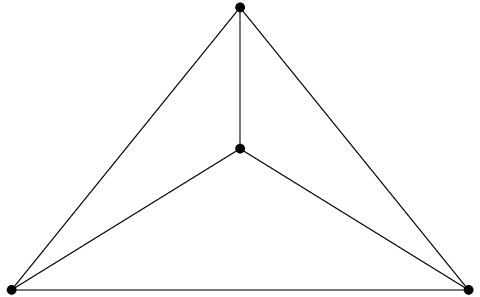
Example 2.6.

We can compute the zeta function of the example shown in figure 3 by using the determinant formula. We obtain $Z_{X}(u)^{-1}=(1-u^{2})^{2}(1-u)(1-2u)(1+u+2u^{2})^{3}$.

Figure 3. A graph

The zeta function has been used to establish some properties of the graphs. For example

Theorem 2.7.

[13, 14, 2, 23, 18] Let $X$ be a finite graph, $r=|EX|-|VX|+1$ the rank of the fundamental group $\pi_{1}(X,x_{0})$. Then $r$ is the order of the pole of $Z_{X}(u)$ at $u=1$. If $r>1$

$$\lim_{u\to 1^{-}}Z_{X}(u)(1-u)^{r}=-\frac{1}{2^{r}(r-1)\kappa_{X}},$$

where $\kappa_{X}$ is the number of spanning trees in $X$.

Theorem 2.8.

[15, 16] Let $X$ be a finite graph, $R_{X}$ be the radius of the greatest circle of convergence of $Z_{X}$. Denote by $\pi_{n}$ the number of prime cycles which have length $n$. If $g.c.d.\{|C|:C\in{\mathcal{P}}\}=1$, then

$$\pi_{n}\sim\frac{R_{X}^{-n}}{n},\ n\to\infty.$$

Theorem 2.9.

[17, 19, 25] Let $X$ be a finite graph which is $(q+1)$-regular, $i.e.$ $\deg(v)=q+1$ for all $v\in VX$. Then the following are equivalent

$(i)$

$$(RH)\ \begin{cases}Z_{X}(q^{-s})^{-1}=0&\\ {\mathcal{R}}s\in(0,1)&\implies{\mathcal{R}}s=\frac{1}{2}.\end{cases}$$

$(ii)$ $X$ is a Ramanujan graph, $i.e.$ $\lambda\in\sigma(A),|\lambda|<q+1\implies|\lambda|\leq 2\sqrt{q}$.

More results on the Ihara zeta function are contained in [24, 26, 27] and in various papers by Mizuno and Sato. In closing this section, we mention a generalization of the Ihara zeta function recently introduced by Bartholdi [1] and studied by Mizuno and Sato (see [20] and references therein).

3. Periodic simple graphs

Let $X=(VX,EX)$ be a simple graph, which we assume to be (countable and) with bounded degree, $i.e.$ the degree of the vertices is uniformly bounded. Let $\Gamma$ be a countable discrete subgroup of automorphisms of $X$, which acts freely on $X$ ($i.e.$ any $\gamma\in\Gamma$, $\gamma\neq id$ doesn’t have fixed points), and with finite quotient $B:=X/\Gamma$. Denote by ${\mathcal{F}}\subset VX$ a set of representatives for $VX/\Gamma$, the vertices of the quotient graph $B$. Let us define a unitary representation of $\Gamma$ on $\ell^{2}(VX)$ by $(\lambda(\gamma)f)(x):=f(\gamma^{-1}x)$, for $\gamma\in\Gamma$, $f\in\ell^{2}(VX)$, $x\in V(X)$. Then the von Neumann algebra ${\mathcal{N}}(X,\Gamma):=\{\lambda(\gamma):\gamma\in\Gamma\}^{\prime}$ of bounded operators on $\ell^{2}(VX)$ commuting with the action of $\Gamma$ inherits a trace given by $Tr_{\Gamma}(T)=\sum_{x\in{\mathcal{F}}}T(x,x)$, for $T\in{\mathcal{N}}(X,\Gamma)$.

Let us denote by $A$ the adjacency matrix of $X$. Then (by [21], [22]) $\|A\|\leq d:=\sup_{v\in VX}\deg(v)<\infty$, and it is easy to see that $A\in{\mathcal{N}}(X,\Gamma)$.

For any $m\in{\mathbb{N}}$, let us denote by $A_{m}(x,y)$ the number of proper paths in $X$, of length $m$, with initial vertex $x$ and terminal vertex $y$, for $x,y\in VX$. Then $A_{1}=A$. Let $A_{0}:=I$ and $Q:=\text{diag}(\deg(v_{1})-1,\deg(v_{2})-1,\ldots)$. Then

Lemma 3.1.

$(i)$ $A_{2}=A^{2}-Q-I\in{\mathcal{N}}(X,\Gamma)$,

$(ii)$ for $m\geq 3$, $A_{m}=A_{m-1}A-A_{m-2}Q\in{\mathcal{N}}(X,\Gamma)$,

$(iii)$ let $\alpha:=\frac{d+\sqrt{d^{2}+4d}}{2}$; then $\|A_{m}\|\leq\alpha^{m}$, for $m\geq 0$.

Proof.

$(i)$ if $x=y$ then $A_{2}(x,x)=0$ because there are no proper closed paths of length $2$ starting at $x$, whereas $A^{2}(x,x)=\deg(x)=(Q+I)(x,x)$, so that $A_{2}(x,x)=A^{2}(x,x)-(Q+I)(x,x)$. If $x\neq y$, then $A^{2}(x,y)$ is the number of paths of length $2$ (necessarily proper) from $x$ to $y$, so $A_{2}(x,y)=A^{2}(x,y)=A^{2}(x,y)-(Q+I)(x,y)$.
$(ii)$ for $x,y\in VX$, the sum $\sum_{z\in VX}A_{m-1}(x,z)A(z,y)$ counts the proper paths of length $m$ from $x$ to $y$, plus additional paths formed of a proper path of length $m-2$ from $x$ to $y$ followed by a path of length $2$ from $y$ to $z$ and back; since the path from $x$ to $y$ and then to $z$ is a proper path of length $m-1$ (one of those counted by $A_{m-1}(x,z))$, $z$ can only be one of the $deg(y)-1=Q(y,y)$ vertices adjacent to $y$, the last one being on the proper path from $x$ to $y$. Therefore $\sum_{z\in VX}A_{m-1}(x,z)A(z,y)=A_{m}(x,y)+A_{m-2}(x,y)Q(y,y)$, and the statement follows.
$(iii)$ We have $\|A_{1}\|=\|A\|\leq d$, $\|A_{2}\|\leq d^{2}+d$, and $\|A_{m}\|\leq d(\|A_{m-1}\|+\|A_{m-2}\|$, from which the claim follows by induction. ∎

Denote by ${\mathcal{C}}_{m}$ the subset of ${\mathcal{C}}$ consisting of the proper closed paths of length $m$, and attach a similar meaning to ${\mathcal{C}}^{\text{tail}}_{m}$, ${\mathcal{C}}^{\text{notail}}_{m}$, ${\mathcal{R}}_{m}$ and ${\mathcal{P}}_{m}$.

Lemma 3.2.

Denote by $t_{m}:=\sum_{x\in{\mathcal{F}}}|\{C\in{\mathcal{C}}^{\text{tail}}_{m}:C\text{ starts at }x\}|$, where $|\cdot|$ denotes the cardinality of a set. Then

$(i)$ $t_{1}=t_{2}=0$, and, for $m\geq 3$, $t_{m}=Tr_{\Gamma}((Q-I)A_{m-2})+t_{m-2}$,

$(ii)$ $t_{m}=Tr_{\Gamma}\left((Q-I)\sum_{j=1}^{[\frac{m-1}{2}]}A_{m-2j}\right)$.

Proof.

$(i)$ Indeed, we have

$$t_{m} =\sum_{x\in{\mathcal{F}}}|\{C\in{\mathcal{C}}^{\text{tail}}_{m}:C\text{ starts at }x\}|$$

$$=\sum_{x\in{\mathcal{F}}}\sum_{y\sim x}|\{C\in{\mathcal{C}}^{\text{tail}}_{m}:C\text{ starts at }x\text{ goes to }y\text{ at first step}\}|$$

$$=\sum_{y\in{\mathcal{F}}}\sum_{x\sim y}|\{C\in{\mathcal{C}}^{\text{tail}}_{m}:C\text{ starts at }x\text{ goes to }y\text{ at first step}\}|,$$

where the last equality follows from the fact that the cardinalities above are $\Gamma$-invariant, and we can choose $\gamma\in\Gamma$ for which the second vertex $y$ of $\gamma C$ is in ${\mathcal{F}}$. A path $C$ in the last set goes from $x$ to $y$, then over a closed path $D$ of length $m-2$, and then back to $x$. There are two kinds of closed paths $D$ at $y$: those with tails and those without. If $D$ has no tail, then there are $Q(y,y)+1$ possibilities for $x$ to be adjacent to $y$, but $x$ cannot be on $D$ (otherwise, $C$ would have backtracking), which leaves $Q(y,y)-1$ possibilities. If $D$ has a tail, $x$ cannot be on $D$ (otherwise, $C$ would have backtracking), which leaves $Q(y,y)$ possibilities. Therefore, we get

$$\sum_{x\sim y}|\{C\in{\mathcal{C}}^{\text{tail}}_{m}:C\text{ starts at }x\text{ goes to }y\text{ at first step}\}|$$

$$=(Q(y,y)-1)\cdot|\{D\in{\mathcal{C}}^{\text{notail}}_{m-2}:D\text{ starts at }y\}|$$

$$\qquad+Q(y,y)\cdot|\{D\in{\mathcal{C}}^{\text{tail}}_{m-2}:D\text{ starts at }y\}|$$

$$=(Q(y,y)-1)\cdot|\{D\in{\mathcal{C}}_{m-2}:D\text{ starts at }y\}|$$

$$\qquad+|\{D\in{\mathcal{C}}^{\text{tail}}_{m-2}:D\text{ starts at }y\}|\,,$$

so that

$$t_{m} =\sum_{y\in{\mathcal{F}}}(Q(y,y)-1)\cdot|\{D\in{\mathcal{C}}_{m-2}:D\text{ starts at }y\}|$$

$$\qquad+\sum_{y\in{\mathcal{F}}}|\{D\in{\mathcal{C}}^{\text{tail}}_{m-2}:D\text{ starts at }y\}|$$

$$=\sum_{y\in{\mathcal{F}}}(Q(y,y)-1)A_{m-2}(y,y)+t_{m-2}$$

$$=Tr_{\Gamma}((Q-I)A_{m-2})+t_{m-2}.$$

$(ii)$ Follows from $(i)$. ∎

We need to introduce an equivalence relation between reduced cycles.

Definition 3.3 (Equivalence relation between reduced cycles).

Given $C$, $D\in{\mathcal{R}}$, we say that $C$ and $D$ are $\Gamma$-equivalent, and write $C\sim_{\Gamma}D$, if there is an isomorphism $\gamma\in\Gamma$ s.t. $D=\gamma(C)$. We denote by $[{\mathcal{R}}]_{\Gamma}$ the set of $\Gamma$-equivalence classes of reduced cycles, and analogously for the subset ${\mathcal{P}}$.

For the purposes of the next result, for any closed path $D=(v_{0},\ldots,v_{m}=v_{0})$, we also denote $v_{j}$ by $v_{j}(D)$.

Let us now assume that $C$ is a prime cycle of length $m$. Then the stabilizer of $C$ in $\Gamma$ is the subgroup $\Gamma_{C}=\{\gamma\in\Gamma:\gamma(C)=C\}$ or, equivalently, $\gamma\in\Gamma_{C}$ if there exists $p(\gamma)\in{\mathbb{Z}}_{m}$ s.t., for any choice of the origin of $C$, $v_{j}(\gamma C)=v_{j-p}(C)$, for any $j$. Let us observe that $p(\gamma)$ is a group homomorphism from $\Gamma_{C}$ to ${\mathbb{Z}}_{m}$, which is injective because $\Gamma$ acts freely. As a consequence, $|\Gamma_{C}|$ divides $m$.

Definition 3.4.

Let $C\in{\mathcal{P}}$ and define $\displaystyle\nu(C):=\frac{|C|}{|\Gamma_{C}|}$. If $C=D^{k}\in{\mathcal{R}}$, where $D\in{\mathcal{P}}$, define $\nu(C)=\nu(D)$. Observe that $\nu(C)$ only depends on $[C]_{\Gamma}\in[{\mathcal{R}}]_{\Gamma}$.

Lemma 3.5.

Let us set $N_{m}:=\sum_{[C]_{\Gamma}\in[{\mathcal{R}}_{m}]_{\Gamma}}\nu(C)$. Then

$(i)$ $N_{m}=Tr_{\Gamma}(A_{m})-t_{m}$,

$(ii)$ $N_{m}\leq d(d-1)^{m-1}|{\mathcal{F}}|$.

Proof.

$(i)$ Let us assume that $[C]_{\Gamma}$ is an equivalence class of prime cycles in $[{\mathcal{P}}_{m}]_{\Gamma}$, and consider the set $U$ of all primitive closed paths with the origin in ${\mathcal{F}}$ and representing $[C]_{\Gamma}$. If $C$ is such a representative, any other representative can be obtained in this way: choose $k\in{\mathbb{Z}}_{m}$, let $\gamma(k)$ be the (unique) element in $\Gamma$ for which $\gamma(k)v_{k}(C)\in{\mathcal{F}}$, and define $C_{k}$ as

$$v_{j}(C_{k})=\gamma(k)v_{j+k}(C),\ j\in{\mathbb{Z}}_{m}.$$

If we want to count the elements of $U$, we should know how many of the elements $C_{k}$ above coincide with $C$. For this to happen, $\gamma$ should clearly be in the stabilizer of the cycle $[C]_{o}$. Conversely, for any $\gamma\in\Gamma_{C}$, there exists $p=p(\gamma)\in{\mathbb{Z}}_{m}$ such that $\gamma v_{j}(C)=v_{j-p}(C)$, therefore $\gamma=\gamma(p)$. As a consequence, $v_{j}(C_{p(\gamma)})=\gamma(p)v_{j+p}(C)=v_{j}(C)$, so that $C_{p(\gamma)}=C$. We have proved that the cardinality of $U$ is equal to $\nu(C)$. The proof for a non-prime cycle is analogous. Therefore,

$$N_{m} =\sum_{[C]_{\Gamma}\in[{\mathcal{R}}_{m}]_{\Gamma}}|\{D\in{\mathcal{C}}^{notail}_{m}:[D]_{o}\sim_{\Gamma}C,v_{0}(D)\in{\mathcal{F}}\}|$$

(3.1) $$=|\{C\in{\mathcal{C}}^{notail}_{m},v_{0}(C)\in{\mathcal{F}}\}|$$

$$=|\{C\in{\mathcal{C}}_{m},v_{0}(C)\in{\mathcal{F}}\}|-|\{C\in{\mathcal{C}}^{tail}_{m},v_{0}(C)\in{\mathcal{F}}\}|$$

$$=Tr_{\Gamma}(A_{m})-t_{m}.$$

$(ii)$ Follows from (3.1).

∎

4. The Zeta function

In this section, we define the Ihara zeta function for a periodic graph, and prove that it is a holomorphic function.

Definition 4.1 (Zeta function).

We let

$$Z_{X,\Gamma}(u):=\prod_{[C]_{\Gamma}\in[{\mathcal{P}}]_{\Gamma}}(1-u^{|C|})^{-\frac{1}{|\Gamma_{C}|}},$$

for all $u\in{\mathbb{C}}$ sufficiently small so that the infinite product converges.

Lemma 4.2.

$(i)$ $Z(u):=\prod_{[C]\in[{\mathcal{P}}]_{\Gamma}}(1-u^{|C|})^{-\frac{1}{|\Gamma_{C}|}}$, defines a holomorphic function in $\{u\in{\mathbb{C}}:|u|<\frac{1}{d-1}\}$,

$(ii)$ $u\frac{Z^{\prime}(u)}{Z(u)}=\sum_{m=1}^{\infty}N_{m}u^{m}$, for $|u|<\frac{1}{d-1}$,

$(iii)$ $Z(u)=\exp\left(\sum_{m=1}^{\infty}\frac{N_{m}}{m}u^{m}\right)$ , for $|u|<\frac{1}{d-1}$.

Proof.

Let us observe that, for $|u|<\frac{1}{d-1}$,

$$\sum_{m=1}^{\infty}N_{m}u^{m} =\sum_{[C]_{\Gamma}\in[{\mathcal{R}}]_{\Gamma}}\nu(C)\,u^{|C|}$$

$$=\sum_{m=1}^{\infty}\sum_{[C]_{\Gamma}\in[{\mathcal{P}}]_{\Gamma}}\frac{|C|}{|\Gamma_{C}|}\,u^{|C^{m}|}$$

$$=\sum_{[C]_{\Gamma}\in[{\mathcal{P}}]_{\Gamma}}\frac{1}{|\Gamma_{C}|}\,\sum_{m=1}^{\infty}|C|u^{|C|m}$$

$$=\sum_{[C]_{\Gamma}\in[{\mathcal{P}}]_{\Gamma}}\frac{1}{|\Gamma_{C}|}\,u\frac{d}{du}\sum_{m=1}^{\infty}\frac{u^{|C|m}}{m}$$

$$=-\sum_{[C]_{\Gamma}\in[{\mathcal{P}}]_{\Gamma}}\frac{1}{|\Gamma_{C}|}\,u\frac{d}{du}\log(1-u^{|C|})$$

$$=u\frac{d}{du}\log Z(u),$$

where, in the last equality we used uniform convergence on compact subsets of $\left\{u\in{\mathbb{C}}:|u|<\frac{1}{d-1}\right\}$. The rest of the proof is clear. ∎

Example 4.3.

Some examples of cycles with different stabilizers are shown in figures 5, 6. They refer to the graph in figure 4 which is the standard lattice graph $X={\mathbb{Z}}^{2}$ endowed with the action of the group $\Gamma$ which is generated by the rotation by $\frac{\pi}{2}$ around the point $P$ and the translations by elements $(m,n)\in{\mathbb{Z}}^{2}$ acting as $(m,n)(v_{1},v_{2}):=(v_{1}+2m,v_{2}+2n)$, for $v=(v_{1},v_{2})\in VX={\mathbb{Z}}^{2}$.

Figure 4. A periodic graph $X$ with its quotient $B=X/\Gamma$

Figure 5. A cycle with $|\Gamma_{C}|=4$

Figure 6. A cycle with $|\Gamma_{C}|=2$

The interested reader can find the computation of the Ihara zeta function for several periodic simple graphs in [9, 4, 5, 6].

5. An analytic determinant for von Neumann algebras with a finite trace

In this section, we define a determinant for a suitable class of not necessarily normal operators in a von Neumann algebra with a finite trace. The results obtained are used in Section 6 to prove a determinant formula for the zeta function.

In a celebrated paper [8], Fuglede and Kadison defined a positive-valued determinant for finite factors ($i.e.$ von Neumann algebras with trivial center and finite trace). Such a determinant is defined on all invertible elements and enjoys the main properties of a determinant function, but it is positive-valued. Indeed, for an invertible operator $A$ with polar decomposition $A=UH$, where $U$ is a unitary operator and $H:=\sqrt{A^{*}A}$ is a positive self-adjoint operator, the Fuglede–Kadison determinant is defined by

$$Det(A)=\exp\,\circ\ \tau\circ\log H,$$

where $\log H$ may be defined via the functional calculus.

For the purposes of the present paper, we need a determinant which is an analytic function. As we shall see, this can be achieved, but corresponds to a restriction of the domain of the determinant function and implies the loss of some important properties. Let $({\mathcal{A}},\tau)$ be a von Neumann algebra endowed with a finite trace. Then, a natural way to obtain an analytic function is to define, for $A\in{\mathcal{A}}$, $\text{det}_{\tau}(A)=\exp\,\circ\ \tau\circ\log A$, where

$$\log(A):=\frac{1}{2\pi i}\int_{\Gamma}\log\lambda(\lambda-A)^{-1}d\lambda,$$

and $\Gamma$ is the boundary of a connected, simply connected region $\Omega$ containing the spectrum of $A$. Clearly, once the branch of the logarithm is chosen, the integral above does not depend on $\Gamma$, provided $\Gamma$ is given as above.

Then a naïve way of defining $det$ is to allow all elements $A$ for which there exists an $\Omega$ as above, and a branch of the logarithm whose domain contains $\Omega$. Indeed the following holds.

Lemma 5.1.

Let $A$, $\Omega$, $\Gamma$ be as above, and $\varphi$, $\psi$ two branches of the logarithm such that both domains contain $\Omega$. Then

$$\exp\,\circ\ \tau\circ\varphi(A)=\exp\,\circ\ \tau\circ\psi(A).$$

Proof.

The function $\varphi(\lambda)-\psi(\lambda)$ is continuous and everywhere defined on $\Gamma$. Since it takes its values in $2\pi i\mathbb{Z}$, it should be constant on $\Gamma$. Therefore

$$\exp\,\circ\ \tau\circ\varphi(A) =\exp\,\circ\ \tau\left(\frac{1}{2\pi i}\int_{\Gamma}2\pi in_{0}(\lambda-A)^{-1}d\lambda\right)\exp\,\circ\ \tau\circ\psi(A)$$

$$=\exp\,\circ\ \tau\circ\psi(A).$$

∎

The problem with the previous definition is its dependence on the choice of $\Omega$. Indeed, it is easy to see that when $A=\begin{pmatrix}1&0\\ 0&i\end{pmatrix}$ and we choose $\Omega$ containing $\{e^{i\vartheta},\vartheta\in[0,\pi/2]\}$ and any suitable branch of the logarithm, we get $det(A)=e^{i\pi/4}$, by using the normalized trace on $2\times 2$ matrices. On the other hand, if we choose $\Omega$ containing $\{e^{i\vartheta},\vartheta\in[\pi/2,2\pi]\}$ and a corresponding branch of the logarithm, we get $det(A)=e^{5i\pi/4}$. Therefore, we make the following choice.

Definition 5.2.

Let $({\mathcal{A}},\tau)$ be a von Neumann algebra endowed with a finite trace, and consider the subset ${\mathcal{A}}_{0}=\{A\in{\mathcal{A}}:0\not\in\text{conv}\,\sigma(A)\}$, where $\sigma(A)$ denotes the spectrum of $A$. For any $A\in{\mathcal{A}}_{0}$ we set

$$\text{det}_{\tau}(A)=\exp\,\circ\ \tau\circ\left(\frac{1}{2\pi i}\int_{\Gamma}\log\lambda(\lambda-A)^{-1}d\lambda\right),$$

where $\Gamma$ is the boundary of a connected, simply connected region $\Omega$ containing $\text{conv}\,\sigma(A)$, and $\log$ is a branch of the logarithm whose domain contains $\Omega$.

Corollary 5.3.

The determinant function defined above is well-defined and analytic on ${\mathcal{A}}_{0}$.

We collect some properties of our determinant in the following result.

Proposition 5.4.

Let $({\mathcal{A}},\tau)$ be a von Neumann algebra endowed with a finite trace, $A\in{\mathcal{A}}_{0}$. Then

$\text{det}_{\tau}(zA)=z^{\tau(I)}\text{det}_{\tau}(A)$, for any $z\in\mathbb{C}\setminus\{0\}$,

if $A$ is normal, and $A=UH$ is its polar decomposition,

$$\text{det}_{\tau}(A)=\text{det}_{\tau}(U)\text{det}_{\tau}(H),$$

if $A$ is positive, $\text{det}_{\tau}(A)=Det(A)$, where the latter is the Fuglede-Kadison determinant.

Proof.

$(i)$ If the half-line $\{\rho e^{i\vartheta_{0}}\in\mathbb{C}:\rho>0\}$ does not intersect $\text{conv}\,\sigma(A)$, then the half-line $\{\rho e^{i(\vartheta_{0}+t)}\in\mathbb{C}:\rho>0\}$ does not intersect $\text{conv}\,\sigma(zA)$, where $z=re^{it}$. If $\log$ is the branch of the logarithm defined on the complement of the real negative half-line, then $\varphi(x)=i(\vartheta_{0}-\pi)+\log(e^{-i(\vartheta_{0}-\pi)}x)$ is suitable for defining $\text{det}_{\tau}(A)$, while $\psi(x)=i(\vartheta_{0}+t-\pi)+\log(e^{-i(\vartheta_{0}+t-\pi)}x)$ is suitable for defining $\text{det}_{\tau}(zA)$. Moreover, if $\Gamma$ is the boundary of a connected, simply connected region $\Omega$ containing $\text{conv}\,\sigma(A)$, then $z\Gamma$ is the boundary of a connected, simply connected region $z\Omega$ containing $\text{conv}\,\sigma(zA)$. Therefore,

$$\text{det}_{\tau}(zA) =\exp\,\circ\ \tau\left(\frac{1}{2\pi i}\int_{z\Gamma}\psi(\lambda)(\lambda-zA)^{-1}d\lambda\right)$$

$$=\exp\,\circ\ \tau\left(\frac{1}{2\pi i}\int_{\Gamma}(i(\vartheta_{0}+t-\pi)+\log(e^{-i(\vartheta_{0}+t-\pi)}re^{it}\mu))(\mu-A)^{-1}d\mu\right)$$

$$=\exp\,\circ\ \tau\left((\log r+it)I+\frac{1}{2\pi i}\int_{\Gamma}\varphi(\mu)(\mu-A)^{-1}d\mu\right)$$

$$=z^{\tau(I)}\text{det}_{\tau}(A).$$

$(ii)$ When $A=UH$ is normal, $U=\int_{[0,2\pi]}e^{i\vartheta}\ du(\vartheta)$, $H=\int_{[0,\infty)}r\ dh(r)$, then $A=\int_{[0,\infty)\times[0,2\pi]}re^{i\vartheta}\ d(h(r)\otimes u(\vartheta))$. The property $0\not\in\text{conv}\,\sigma(A)$ is equivalent to the fact that the support of the measure $d(h(r)\otimes u(\vartheta))$ is compactly contained in some open half-plane

$$\{\rho e^{i\vartheta}:\rho>0,\vartheta\in(\vartheta_{0}-\pi/2,\vartheta_{0}+\pi/2)\},$$

or, equivalently, that the support of the measure $dh(r)$ is compactly contained in $(0,\infty)$, and the support of the measure $du(\vartheta)$ is compactly contained in $(\vartheta_{0}-\pi/2,\vartheta_{0}+\pi/2)$. Therefore $A\in{\mathcal{A}}_{0}$ is equivalent to $U,H\in{\mathcal{A}}_{0}$. Then

$$\log A=\int_{[0,\infty)\times(\vartheta_{0}-\pi/2,\vartheta_{0}+\pi/2)}(\log r+i\vartheta)\ d(h(r)\otimes u(\vartheta)),$$

which implies that

$$\text{det}_{\tau}(A) =\exp\,\circ\ \tau\left(\int_{0}^{\infty}\log r\ dh(r)+\int_{\vartheta_{0}-\pi/2}^{\vartheta_{0}+\pi/2}i\vartheta\ du(\vartheta)\right)$$

$$=\text{det}_{\tau}(U)\cdot\text{det}_{\tau}(H).$$

$(iii)$ Follows by the above argument. ∎

Remark 5.5.

We note that the above defined determinant function strongly violates the product property $\text{det}_{\tau}(AB)=\text{det}_{\tau}(A)\text{det}_{\tau}(B)$. Indeed, the fact that $A,B\in{\mathcal{A}}_{0}$ does not imply $AB\in{\mathcal{A}}_{0}$, as is seen e.g. by taking $A=B=\begin{pmatrix}1&0\\ 0&i\end{pmatrix}$. Moreover, even if $A,B,AB\in{\mathcal{A}}_{0}$ and $A$ and $B$ commute, the product property may be violated, as is shown by choosing $A=B=\begin{pmatrix}1&0\\ 0&e^{3i\pi/4}\end{pmatrix}$, and using the normalized trace on $2\times 2$ matrices.

6. The determinant formula

In this section, we prove the main result in the theory of Ihara zeta functions, which says that $Z$ is the reciprocal of a holomorphic function, which, up to a factor, is the determinant of a deformed Laplacian on the graph. We first need some technical results. Let us recall that $d:=\sup_{v\in VX}\deg(v)$, and $\alpha:=\frac{d+\sqrt{d^{2}+4d}}{2}$.

Lemma 6.1.

$(i)$ $\left(\sum_{m\geq 0}A_{m}u^{m}\right)(I-Au+Qu^{2})=(1-u^{2})I$, for $|u|<\frac{1}{\alpha}$,

$(ii)$ $\left(\sum_{m\geq 0}\left(\sum_{k=0}^{[m/2]}A_{m-2k}\right)u^{m}\right)(I-Au+Qu^{2})=I$, for $|u|<\frac{1}{\alpha}$.

Proof.

$(i)$ From Lemma 3.1 we obtain

$$\biggl(\sum_{m\geq 0}A_{m}u^{m}\biggr) (I-Au+Qu^{2})=\sum_{m\geq 0}A_{m}u^{m}-\sum_{m\geq 0}\left(A_{m}Au^{m+1}-A_{m}Qu^{m+2}\right)$$

$$=\sum_{m\geq 0}A_{m}u^{m}-A_{0}Au-A_{1}Au^{2}+A_{0}Qu^{2}$$

$$\qquad-\sum_{m\geq 3}\left(A_{m-1}A-A_{m-2}Q\right)u^{m}$$

$$=\sum_{m\geq 0}A_{m}u^{m}-Au-A^{2}u^{2}+Qu^{2}-\sum_{m\geq 3}A_{m}u^{m}$$

$$=I+Au+A_{2}u^{2}-Au-A^{2}u^{2}+Qu^{2}$$

$$=(1-u^{2})I.$$

$(ii)$

$$I =(1-u^{2})^{-1}\biggl(\sum_{m\geq 0}A_{m}u^{m}\biggr)(I-Au+Qu^{2})$$

$$=\biggl(\sum_{m\geq 0}A_{m}u^{m}\biggr)\biggl(\sum_{j=0}^{\infty}u^{2j}\biggr)(I-Au+Qu^{2})$$

$$=\biggl(\sum_{k\geq 0}\sum_{j=0}^{\infty}A_{k}u^{k+2j}\biggr)(I-Au+Qu^{2})$$

$$=\biggl(\sum_{m\geq 0}\biggl(\sum_{j=0}^{[m/2]}A_{m-2j}\biggr)u^{m}\biggr)(I-Au+Qu^{2}).$$

∎

Lemma 6.2.

Denote by $B_{m}:=A_{m}-(Q-I)\sum_{k=1}^{[m/2]}A_{m-2k}\in{\mathcal{N}}(X,\Gamma)$, for $m\geq 0$. Then

$(i)$ $B_{0}=I$, $B_{1}=A$,

$(ii)$ $B_{m}=QA_{m}-(Q-I)\sum_{k=0}^{[m/2]}A_{m-2k}$,

$(iii)$

$$Tr_{\Gamma}B_{m}=\begin{cases}N_{m}-Tr_{\Gamma}(Q-I)&m\text{ even}\\ N_{m}&m\text{ odd,}\end{cases}$$

$(iv)$

$$\sum_{m\geq 1}B_{m}u^{m}=\left(Au-2Qu^{2}\right)\left(I-Au+Qu^{2}\right)^{-1},\ \text{ for }|u|<\frac{1}{\alpha}.$$

Proof.

$(i)$, $(ii)$ follow from computations involving bounded operators.

$(iii)$ It follows from Lemma 3.2 $(ii)$ that, if $m$ is odd,

$$Tr_{\Gamma}B_{m}=Tr_{\Gamma}(A_{m})-t_{m}=N_{m},$$

whereas, if $m$ is even,

$$Tr_{\Gamma}B_{m}=Tr_{\Gamma}(A_{m})-t_{m}-Tr_{\Gamma}((Q-I)A_{0})=N_{m}-Tr_{\Gamma}(Q-I).$$

$(iv)$

$$\biggl(\sum_{m\geq 0}B_{m}u^{m}\biggr) (I-Au+Qu^{2})$$

$$=\biggl(Q\sum_{m\geq 0}A_{m}u^{m}-(Q-I)\sum_{m\geq 0}\sum_{j=0}^{[m/2]}A_{m-2j}u^{m}\biggr)(I-Au+Qu^{2})$$

$$=Q(1-u^{2})I-(Q-I)\biggl(\sum_{m\geq 0}\sum_{j=0}^{[m/2]}A_{m-2j}u^{m}\biggr)(I-Au+Qu^{2})$$

$$=(1-u^{2})Q-(Q-I)=I-u^{2}Q,$$

where the second equality follows by Lemma 6.1 $(i)$ and the third equality follows by Lemma 6.1 $(ii)$. Since $B_{0}=I$, we get

$$\biggl(\sum_{m\geq 1}B_{m}u^{m}\biggr)(I-Au+Qu^{2}) =I-u^{2}Q-B_{0}(I-Au+Qu^{2})$$

$$=Au-2Qu^{2}.$$

∎

Lemma 6.3.

Let $f:u\in B_{\varepsilon}\equiv\{u\in{\mathbb{C}}:|u|<\varepsilon\}\mapsto f(u)\in{\mathcal{N}}(X,\Gamma)$, be a $C^{1}$- function, $f(0)=0$, and $\|f(u)\|<1$, for all $u\in B_{\varepsilon}$. Then

$$Tr_{\Gamma}\left(-\frac{d}{du}\log(I-f(u))\right)=Tr_{\Gamma}\left(f^{\prime}(u)(I-f(u))^{-1}\right).$$

Proof.

To begin with, $-\log(I-f(u))=\sum_{n\geq 1}\frac{1}{n}f(u)^{n}$, converges in operator norm, uniformly on compact subsets of $B_{\varepsilon}$. Moreover,

$$\frac{d}{du}f(u)^{n}=\sum_{j=0}^{n-1}f(u)^{j}f^{\prime}(u)f(u)^{n-j-1}.$$

Therefore, $-\frac{d}{du}\log(I-f(u))=\sum_{n\geq 1}\frac{1}{n}\sum_{j=0}^{n-1}f(u)^{j}f^{\prime}(u)f(u)^{n-j-1}$, so that

$$Tr_{\Gamma}\biggl(-\frac{d}{du}\log(I-f(u))\biggr) =\sum_{n\geq 1}\frac{1}{n}\sum_{j=0}^{n-1}Tr_{\Gamma}\left(f(u)^{j}f^{\prime}(u)f(u)^{n-j-1}\right)$$

$$=\sum_{n\geq 1}Tr_{\Gamma}(f(u)^{n-1}f^{\prime}(u))$$

$$=Tr_{\Gamma}\biggl(\sum_{n\geq 0}f(u)^{n}f^{\prime}(u)\biggr)$$

$$=Tr_{\Gamma}(f^{\prime}(u)(I-f(u))^{-1}),$$

where we have used the fact that $Tr_{\Gamma}$ is norm continuous. ∎

Corollary 6.4.

$$Tr_{\Gamma}\left(\sum_{m\geq 1}B_{m}u^{m}\right)=Tr_{\Gamma}\left(-u\frac{d}{du}\log(I-Au+Qu^{2})\right),\ |u|<\frac{1}{\alpha}.$$

Proof.

It follows from Lemma 6.2 $(iv)$ that

$$Tr_{\Gamma}\biggl(\sum_{m\geq 1}B_{m}u^{m}\biggr) =Tr_{\Gamma}((Au-2Qu^{2})(I-Au+Qu^{2})^{-1})$$

$$=Tr_{\Gamma}\Bigl(-u\frac{d}{du}\log(I-Au+Qu^{2})\Bigr),$$

where the last equality follows from the previous lemma applied with $f(u):=Au-Qu^{2}$. ∎

Observe that for the $L^{2}$-Euler characteristic of $X$ we have

$$\chi^{(2)}(X):=-\frac{1}{2}Tr_{\Gamma}(Q-I)=|V(B)|-|E(B)|=\chi(B),$$

where $\chi(B)$ is the Euler characteristic of the quotient graph $B=X/\Gamma$.

Theorem 6.5 (Determinant formula).

$$\frac{1}{Z_{X,\Gamma}(u)}=(1-u^{2})^{-\chi(B)}\text{det}_{\Gamma}(I-Au+Qu^{2}),\ \text{ for }|u|<\frac{1}{\alpha}.$$

Proof.

$$Tr_{\Gamma}\biggl(\sum_{m\geq 1}B_{m}u^{m}\biggr) =\sum_{m\geq 1}Tr_{\Gamma}(B_{m})u^{m}$$

$$=\sum_{m\geq 1}N_{m}u^{m}-\sum_{k\geq 1}Tr_{\Gamma}(Q-I)u^{2k}$$

$$=\sum_{m\geq 1}N_{m}u^{m}-Tr_{\Gamma}(Q-I)\frac{u^{2}}{1-u^{2}},$$

where the second equality follows by Lemma 6.2 $(iii)$. Therefore,

$$u\frac{d}{du}\log Z_{X,\Gamma}(u) =\sum_{m\geq 1}N_{m}u^{m}$$

$$=Tr_{\Gamma}\left(-u\frac{d}{du}\log(I-Au+Qu^{2})\right)-\frac{u}{2}\frac{d}{du}\log(1-u^{2})Tr_{\Gamma}(Q-I)$$

so that, dividing by $u$ and integrating from $u=0$ to $u$, we get

$$\log Z_{X,\Gamma}(u)=-Tr_{\Gamma}\left(\log(I-Au+Qu^{2})\right)-\frac{1}{2}Tr_{\Gamma}(Q-I)\log(1-u^{2}),$$

which implies that, for $|u|<\frac{1}{\alpha}$, we have

$$\frac{1}{Z_{X,\Gamma}(u)}=(1-u^{2})^{\frac{1}{2}Tr_{\Gamma}(Q-I)}\cdot\exp Tr_{\Gamma}\log(I-Au+Qu^{2}).$$

∎

7. Functional equations

In this final section, we obtain several functional equations for the Ihara zeta functions of $(q+1)-$regular graphs, $i.e.$ graphs with $\deg(v)=q+1$, for any $v\in VX$. The various functional equations correspond to different ways of completing the zeta functions, as is done in [25] for finite graphs.

Lemma 7.1.

Let $X$ be a $(q+1)$-regular graph and $\Delta(u):=(1+qu^{2})I-uA$. Then

$(i)$ $\chi^{(2)}(X)=\chi(B)=|V(B)|(1-q)/2\in{\mathbb{Z}}$,

$(ii)$ $\displaystyle Z_{X,\Gamma}(u)=(1-u^{2})^{\chi(B)}\text{det}_{\Gamma}(\Delta(u))^{-1}$, for $|u|<\frac{1}{q}$,

$(iii)$ by using the determinant formula in $(ii)$, $Z_{X,\Gamma}$ can be extended to a function holomorphic at least in the open set

$$\Omega:={\mathbb{R}}^{2}\setminus\left(\left\{(x,y)\in{\mathbb{R}}^{2}:x^{2}+y^{2}=\frac{1}{q}\right\}\cup\left\{(x,0)\in{\mathbb{R}}^{2}:\frac{1}{q}\leq|x|\leq 1\right\}\right).$$

See figure 7.

Figure 7. The open set $\Omega$

$(iv)$ $\displaystyle\text{det}_{\Gamma}\Bigl(\Delta(\frac{1}{qu})\Bigr)=(qu^{2})^{-|VB|}\text{det}_{\Gamma}(\Delta(u))$, for $u\in\Omega\setminus\left\{0\right\}$.

Proof.

$(i)$ This follows by a simple computation.

$(ii)$ This follows from $(i)$.

$(iii)$ Let us observe that

$$\sigma(\Delta(u))=\left\{1+qu^{2}-u\lambda:\lambda\in\sigma(A)\right\}\subset\left\{1+qu^{2}-u\lambda:\lambda\in[-d,d]\right\}.$$

It follows that $0\not\in\text{conv}\,\sigma(\Delta(u))$ at least for $u\in{\mathbb{C}}$ such that $1+qu^{2}-u\lambda\neq 0$ for $\lambda\in[-d,d]$, that is for $u=0$ or $\frac{1+qu^{2}}{u}\not\in[-d,d]$, or equivalently, at least for $u\in\Omega$. The rest of the proof follows from Corollary 5.3.

$(iv)$ This follows by Proposition 5.4 $(i)$ and the fact that $Tr_{\Gamma}(I_{V})=|VB|$. ∎

Proposition 7.2 (Functional equations).

Let $X$ be $(q+1)$-regular. Then, for all $u\in\Omega$, we have

$(i)$ $\Lambda_{X,\Gamma}(u):=(1-u^{2})^{-\chi(B)}(1-u^{2})^{|VB|/2}(1-q^{2}u^{2})^{|VB|/2}Z_{X,\Gamma}(u)=-\Lambda_{X,\Gamma}\Bigl(\frac{1}{qu}\Bigr)$,

$(ii)$ $\xi_{X,\Gamma}(u):=(1-u^{2})^{-\chi(B)}(1-u)^{|VB|}(1-qu)^{|VB|}Z_{X,\Gamma}(u)=\xi_{X,\Gamma}\Bigl(\frac{1}{qu}\Bigr)$,

$(iii)$ $\Xi_{X,\Gamma}(u):=(1-u^{2})^{-\chi(B)}(1+qu^{2})^{|VB|}Z_{X,\Gamma}(u)=\Xi_{X,\Gamma}\Bigl(\frac{1}{qu}\Bigr)$.

Proof.

$(i)$

$$\Lambda_{X}(u) =(1-u^{2})^{|VB|/2}(1-q^{2}u^{2})^{|VB|/2}\text{det}_{\Gamma}(\Delta(u))^{-1}$$

$$=u^{|VB|}\Bigl(\frac{q^{2}}{q^{2}u^{2}}-1\Bigr)^{|VB|/2}(qu)^{|VB|}\Bigl(\frac{1}{q^{2}u^{2}}-1\Bigr)^{|VB|/2}\frac{1}{(qu^{2})^{|VB|}}\text{det}_{\Gamma}\Bigl(\Delta(\frac{1}{qu})\Bigr)^{-1}$$

$$=-\Lambda_{X}\Bigl(\frac{1}{qu}\Bigr).$$

$(ii)$

$$\xi_{X}(u) =(1-u)^{|VB|}(1-qu)^{|VB|}\text{det}_{\Gamma}(\Delta(u))^{-1}$$

$$=u^{|VB|}\Bigl(\frac{q}{qu}-1\Bigr)^{|VB|}(qu)^{|VB|}\Bigl(\frac{1}{qu}-1\Bigr)^{|VB|}\frac{1}{(qu^{2})^{|VB|}}\text{det}_{\Gamma}\Bigl(\Delta(\frac{1}{qu})\Bigr)^{-1}$$

$$=\xi_{X}\Bigl(\frac{1}{qu}\Bigr).$$

$(iii)$

$$\Xi_{X}(u) =(1+qu^{2})^{|VB|}\text{det}_{\Gamma}(\Delta(u))^{-1}$$

$$=(qu^{2})^{|VB|}\Bigl(\frac{q}{q^{2}u^{2}}+1\Bigr)^{|VB|}\frac{1}{(qu^{2})^{|VB|}}\text{det}_{\Gamma}\Bigl(\Delta(\frac{1}{qu})\Bigr)^{-1}$$

$$=\Xi_{X}\Bigl(\frac{1}{qu}\Bigr).$$

∎

Acknowledgement .

The second and third named authors would like to thank respectively the University of California, Riverside, and the University of Roma “Tor Vergata” for their hospitality at different stages of the preparation of this paper.

References

• [1] L. Bartholdi. Counting paths in graphs, Enseign. Math. 45 (1999), 83–131.
• [2] H. Bass. The Ihara-Selberg zeta function of a tree lattice, Internat. J. Math. 3 (1992), 717–797.
• [3] H. Bass, A. Lubotzky. Tree lattices, Progress in Math. 176, Birkhäuser, Boston, 2001.
• [4] B. Clair, S. Mokhtari-Sharghi. Zeta functions of discrete groups acting on trees, J. Algebra 237 (2001), 591–620.
• [5] B. Clair, S. Mokhtari-Sharghi. Convergence of zeta functions of graphs, Proc. Amer. Math. Soc. 130 (2002), 1881–1886.
• [6] B. Clair. Zeta functions of graphs with ℤ{\mathbb{Z}} actions, preprint, 2006, arXiv:math.NT/0607689.
• [7] D. Foata, D. Zeilberger. A combinatorial proof of Bass’s evaluations of the Ihara-Selberg zeta function for graphs, Trans. Amer. Math. Soc. 351 (1999), 2257–2274.
• [8] B. Fuglede, R. V. Kadison. Determinant theory in finite factors, Ann. Math. 55 (1952), 520-530.
• [9] R. I. Grigorchuk, A. Z˙\dot{\text{Z}}uk. The Ihara zeta function of infinite graphs, the KNS spectral measure and integrable maps, in: “Random Walks and Geometry”, Proc. Workshop (Vienna, 2001), V. A. Kaimanovich et al., eds., de Gruyter, Berlin, 2004, pp. 141–180.
• [10] D. Guido, T. Isola, M. L. Lapidus. A trace on fractal graphs and the Ihara zeta function, preprint, 2006, arXiv:math.OA/0608060.
• [11] D. Guido, T. Isola, M. L. Lapidus. Ihara’s zeta function for periodic graphs and its approximation in the amenable case, preprint, 2006, arXiv:math.OA/0608229.
• [12] K. Hashimoto, A. Hori. Selberg-Ihara’s zeta function for pp-adic discrete groups, in: “Automorphic Forms and Geometry of Arithmetic Varieties”, Adv. Stud. Pure Math. 15, Academic Press, Boston, MA, 1989, pp. 171–210.
• [13] K. Hashimoto. Zeta functions of finite graphs and representations of pp-adic groups, in: “Automorphic Forms and Geometry of Arithmetic Varieties”, Adv. Stud. Pure Math. 15, Academic Press, Boston, MA, 1989, pp. 211–280.
• [14] K. Hashimoto. On zeta and L-functions of finite graphs, Internat. J. Math. 1 (1990), 381–396.
• [15] K. Hashimoto. Artin type L-functions and the density theorem for prime cycles on finite graphs, Internat. J. Math. 3 (1992), 809–826.
• [16] M. D. Horton, H. M. Stark, A. A. Terras. What are zeta functions of graphs and what are they good for?, preprint.
• [17] Y. Ihara. On discrete subgroups of the two by two projective linear group over 𝔭\mathfrak{p}-adic fields, J. Math. Soc. Japan 18 (1966), 219–235.
• [18] M. Kotani, T. Sunada. Zeta functions of finite graphs, J. Math. Sci. Univ. Tokyo 7 (2000), 7–25.
• [19] A. Lubotzky. Discrete groups, expanding graphs and invariant measures, Progress in Math. 125, Birkhäuser, Basel, 1994.
• [20] H. Mizuno, I. Sato. Bartholdi zeta functions of some graphs, Discrete Math. 206 (2006), 220-230.
• [21] B. Mohar. The spectrum of an infinite graph, Linear Algebra Appl. 48 (1982), 245-256.
• [22] B. Mohar, W. Woess. A survey on spectra of infinite graphs, Bull. London Math. Soc. 21 (1989), 209-234.
• [23] S. Northshield. A note on the zeta function of a graph, J. Combin. Theory Series B 74 (1998), 408–410.
• [24] J. P. Serre. Répartition asymptotique des valeurs propres de l’opérateur de Hecke TpT_{p}, J. Amer. Math. Soc. 10 (1997), 75–102.
• [25] H. M. Stark, A. A. Terras. Zeta functions of finite graphs and coverings, Adv. Math. 121 (1996), 126-165.
• [26] H. M. Stark, A. A. Terras. Zeta functions of finite graphs and coverings. II, Adv. Math. 154 (2000), 132–195.
• [27] H. M. Stark, A. A. Terras. Zeta functions of finite graphs and coverings. III, to appear in Adv. Math.
• [28] T. Sunada. L-functions in geometry and applications, Springer Lecture Notes in Math. 1201, 1986, pp. 266-284.