On the Density of Iterated Line Segment Intersections

Abstract

Given $S_{1}$, a finite set of points in the plane, we define a sequence of point sets ${S_{i}}$ as follows: With $S_{i}$ already determined, let $L_{i}$ be the set of all the line segments connecting pairs of points of $\bigcup_{j=1}^{i}S_{j}$, and let $S_{i+1}$ be the set of intersection points of those line segments in $L_{i}$, which cross but do not overlap. We show that with the exception of some starting configurations the set of all crossing points $\bigcup_{i=1}^{\infty}S_{i}$ is dense in a particular subset of the plane with nonempty interior. This region is the intersection of all closed half planes which contain all but at most one point from $S_{1}$.

Keywords: discrete geometry, computational geometry, density, intersections, line segments

1 Introduction

Given $S=S_{1}$, a finite set of points in the Euclidean plane, let $L_{1}$ denote the set of line segments connecting pairs of points from $S_{1}$. Next, let $S_{2}$ be the set of all the intersection points of those line segments in $L_{1}$ which do not overlap. We continue to define sets of line segments $L_{i}$ and point sets $S_{i}$ inductively by

$$L_{i} := \bigg\{pq\;\bigg|\;p,q\in\bigcup_{j=1}^{i}S_{j}\;\wedge\;\;p\neq q\bigg\},$$

$$S_{i+1} := \left\{x\;|\;\{x\}=l\cap l^{\prime}\mbox{ where }l,l^{\prime}\in L_{i}\right\}.$$

Finally, let $S_{\infty}:=\bigcup_{i=1}^{\infty}S_{i}$ denote the limit set.

Figure 1: The first iterations $S_{1}$, $S_{2}$ and $S_{3}$ of segment intersections.

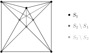
In this article we show which starting configurations $S$ give rise to density of $S_{\infty}$. And for those, we prove that $S_{\infty}$ is dense in a certain region $K(S)$.

Several results concerning the density of similar iterated constructions are known. Bezdek and Pach [2] studied the following problem: Let $S_{1}=\{O_{1},O_{2}\}$ consist of two distinct points in the plane with distance less than $2$. Define $S_{i+1}$ inductively as the set of all intersection points between the unit circles, whose centers are in $S_{i}$. They proved, if the distance between $O_{1}$ and $O_{2}$ does not equal $1$ nor $\sqrt{3}$, the limit point set $\bigcup_{i=1}^{\infty}S_{i}$ is everywhere dense in the plane.

Kazdan [8] considered two rigid motions $A$ and $B$ applied to an arbitrary point $p$ in the plane. An implication of his more powerful result is that the set $S_{\infty}:=\bigcup_{i=1}^{\infty}S_{i}$ defined by the iterations $S_{1}:=\{p\}$ and $S_{i+1}$ $:=$ $\{Ax,$ $A^{-1}x,$ $Bx,$ $B^{-1}x|x\in S_{i}\}$ is everywhere dense in the plane if $A$ is a rotation through an angle incommensurable with $2\pi$ and $A$ and $B$ do not commute.

Bárány, Frankl, and Maehara [1] showed that with the exception of four special cases, the set of vertices of those triangles which are obtained from a particular starting triangle $T$ by repeated edge-reflection is everywhere dense in the plane.

Ismailescu and Radoičić [7] examined a question very similar to ours. The only difference is that they considered lines instead of line segments. They proved by applying nice elementary methods that with the exception of two cases the crossing points are dense in the whole plane. Hillar and Rhea [6] independently proved the same statement with different methods.

Despite the similarity of the two settings, the methods from the analysis of iterated line intersections cannot be transferred to our case of segment intersections. The latter problem turns out to be more difficult. It has more exceptional cases, where the crossing points are not dense in any set with non-empty interior. And in non-exceptional cases the crossing points are not dense in the whole plane but only in a particular convex region $K(S)$. In fact, if we do not consider exceptional configurations, the line result is a direct consequence of the segment result presented here. If the iterated intersections of line segments are dense in a region with non-empty interior, clearly, the intersections of lines starting with the same point set are dense in the same region and thereby in the whole plane.

Our work is motivated by another interesting problem introduced recently by Ebbers-Baumann et al. [4]; namely how to embed a given finite point set into a geometric graph of small dilation. Here a geometric graph is a graph in the Euclidean plane, where the vertices are points in the plane, the edges are rectifiable curves connecting the two adjacent vertices, and the edge lengths equal the lengths of the corresponding curves. Given such a geometric graph $G$, for any two vertices $p$ and $q$ we define their vertex-to-vertex dilation as

$$\delta_{G}(p,q):=\displaystyle\frac{|\pi(p,q)|}{|pq|},$$

where $\pi(p,q)$ is a shortest path from $p$ to $q$ in $G$ and $|\,.\,|$ denotes the Euclidean length. The dilation of $G$ is defined by

$$\delta(G):=\sup_{\mbox{\scriptsize$p$, $q$ vertices of $G$},\;p\neq q}\delta_{G}(p,q).$$

A geometric graph $G$ of smallest possible dilation $\delta(G)=1$ is called dilation-free. We will give a list of all cases of dilation-free planar graphs in Section 2. It can also be found at Eppstein’s geometry junkyard [5]. Given a point set $S$ in the plane, the dilation of $S$ is defined by

$$\Delta(S):=\inf\left\{\;\delta(G)\;\left|\;G=(V,E)\mbox{ planar graph},\;S\subseteq V\mbox{ and }V\setminus S\mbox{ finite }\right\}\right..$$

Determining $\Delta(S)$ seems to be very difficult. The answer is even unknown if $S$ is a set of five points placed evenly on a circle. However, Ebbers-Baumann et al. [4] were able to prove $\Delta(S)\leq 1.1247$ for every finite point set $S\subset\mathbb{R}^{2}$ and they showed lower bounds for some special cases.

A natural idea for embedding $S$ in a planar graph of small dilation is to try to find a geometric graph $G=(V,E)$, $S\subseteq V$, such that $\delta_{G}(p,q)=1$ for every $p,q\in V$. Now, suppose we have found such $G$. Obviously, for every pair $p,q\in S$, the line segment $pq$ must be a part of $G$. Since $G$ must be planar, every intersection point of these line segments must also be in $V$ and so on.

If this iteration produces only finitely many intersection points, i.e. the set $S_{\infty}$ defined at the very beginning of this article is finite, we have a planar graph $G=(V,E)$ with $S\subseteq V$, $|V\setminus S|<\infty$ and $\delta(G)=1$; thus $\Delta(S)=1$. This shows that $|S_{\infty}|<\infty$ can only hold if $S$ is a subset of the vertices of a dilation-free planar graph. We call those point sets exceptional configurations. Note that $\Delta(S)=1$ could still hold for other sets. There could be a sequence of proper geometric graphs whose dilation does not equal $1$ but converges to $1$.

Our main result is the following.

Theorem 1.

Let $S=S_{1}$ be a set of $n$ points in the plane, which is not an exceptional configuration. Then $S_{\infty}$ is dense in the region $K(S)$.

The region $K(S)$ can be described by the following simple definition. An example is shown in Figure 2. Until we prove that $S_{\infty}$ is indeed dense in $K(S)$, we call $K(S)$ the candidate.

Figure 2: The candidate $K(S)$ and a closed half plane $H$ containing all but one starting point.

Definition.

The candidate $K(S)$ is defined as the intersection of those closed half planes which contain all the starting points except for at most one point,

$$K(S):=\bigcap_{p\in S}\,\bigcap_{H\supset S\setminus\{p\}}H.$$

The second intersection is taken over all closed half planes $H$ which contain $S\setminus\{p\}$.

After the first version of our proof was worked out, Klein and Kutz [9] used the statement of Theorem 1 to prove the first non-trivial lower bound $\Delta(S)\geq 1.0000047$ which holds for every non-exceptional finite point set $S$. They also sketched a different proof for the special case of Theorem 1 where $S$ consists of more than four points in convex position, not three of them on a line. The proof is based on a convergence argument similar in spirit to our Lemma 9 and on bounds to distance ratios between the converging points.

The rest of this paper is organized as follows. In Section 2 we list the exceptional configurations and we show basic properties of $K(S)$. In Section 3 we study a special case of the problem. In Section 4 we use arguments from projective geometry to prove for any non-exceptional configuration $S$ that there exists a triangle $T$ such that $S_{\infty}$ is dense in $T$. Finally, in the last section we prove that in this case $S_{\infty}$ is dense in $K(S)$.

2 Exceptional configurations and the candidate

Here, we list all cases of dilation-free graphs. They can also be found at Eppstein’s Geometry Junkyard [5]. It can be proven by case analysis that these are all possibilities. The exceptional configurations are the subsets of the vertices of such graphs. Most exceptional configurations are the whole vertex set of a corresponding dilation-free graph. Only the special case described in the footnote in ($iii$) yields an exceptional configuration which is a proper subset.

The main statement we want to prove in this paper is that if $S$ is not an exceptional configuration, the set $S_{\infty}$ is dense in the candidate $K(S)$. As a first step, we list some basic properties of $K(S)$ in the following lemma. The most important one is that there cannot be any intersection point outside the candidate.

Lemma 2.

2. If the candidate $K(S)$ is not empty, it is a convex polygon.

3. Every vertex of $K(S)$ belongs to $S_{1}\cup S_{2}$.

4. Every intersection point lies inside of the candidate, that is $S_{\infty}\setminus S\subseteq K(S)$.

Proof.

1. The convexity follows immediately from the definition because $K(S)$ is the intersection of (convex) closed half planes. The definition also implies that $K(S)$ is a subset of the convex hull $\mathrm{ch}(S)$. It is bounded. Furthermore, it is easy to see that in the definition of the candidate it suffices to consider only those finitely many closed half planes $H$ which have at least two points from $S$ on their boundary. Hence, $K(S)$ is a polygon.

Figure 3: Every vertex $v$ of the candidate $K(S)$ has to be an element of $S_{1}\cup S_{2}$.

2. Consider Figure 3. Let $e_{1}$ and $e_{2}$ be two neighbor edges of the polygon $K(S)$ meeting in the vertex $v$, and let $\ell_{1}$ and $\ell_{2}$ be the lines through these edges. By the arguments above there are at least two points from $S$ on each of the lines. If there are two points $p_{1},q_{1}\in S$ on $\ell_{1}$ on opposite sides of $\ell_{2}$, and there are two points $p_{2},q_{2}\in S$ on $\ell_{2}$ on opposite sides of $\ell_{1}$, then, as shown in Figure 3.a, the vertex $v$ belongs to $S_{2}$ since it is the crossing point of $p_{1}q_{1}$ and $p_{2}q_{2}$.

Otherwise all points of $S\cap\ell_{1}$ lie on one side of $\ell_{2}$ or all points of $S\cap\ell_{2}$ lie on one side of $\ell_{1}$. We assume the first situation, which is depicted in Figure 3.b. Let $p_{1}$ be the point in $S\cap\ell_{1}$ which is closest to $v$. Then, if $v$ is not a point of $S=S_{1}$, we can rotate the half plane $H_{1}$ belonging to $e_{1}$ around $p_{1}$ such that the turned closed half plane $\tilde{H}_{1}$ still contains all but one point of $S$ and it does not contain $v\in K(S)$. This is a contradiction because by definition $K(S)$ would have to be contained in $\tilde{H}_{1}$.

3. Let $H$ be a closed half plane containing $S\setminus\{p\}$. Then, clearly the crossing points of the next generation $S_{2}\setminus S$ are contained in $H$, since all the line segments connecting points from $S$ are either fully contained in $H$ or they meet in $p$. Applying this argument inductively shows that $S_{\infty}\setminus S\subset H$. ∎

3 A useful special case

In this whole section we consider a starting configuration $S=\{A,B,C,D,E,F\}$ as shown in Figure 4. The three points $A$, $B$, $C$ are not collinear, and the three remaining points $D$, $E$, $F$ are the midpoints of the segments $A\hskip-1.00006ptB$, $B\hskip-1.00006ptC$ and $A\hskip-1.00006ptC$ respectively. We want to prove the main statement for this special case. This means, we want to show that for such a starting configuration the set of intersection points $S_{\infty}$ is dense in the triangle $\mbox{\large$\bigtriangleup$}DEF$.

Figure 4: Proving that the intersection points are dense in the triangle $\mbox{\large$\bigtriangleup$}DEF$.

In order to do so, it is sufficient to show that $S_{\infty}$ is dense on the sides of this triangle because in this case the intersections of the segments connecting the points on the sides are dense in the interior of the triangle.

Actually, for the proof we consider only a particular subset $\tilde{S}_{\infty}\subseteq S_{\infty}$. Let ${\cal T}:=D\hskip-1.00006ptE\cup E\hskip-1.00006ptF\cup D\hskip-1.00006ptF$ denote the boundary of the triangle $\mbox{\large$\bigtriangleup$}{DEF}$. Now, in each step of the iteration we consider only segments which connect points on ${\cal T}$ with a vertex from $\{A,B,C\}$, and the intersections of such segments with ${\cal T}$. More formally we define

$$\tilde{S}_{0}:=\{D,E,F\},\;\;\;\;\forall i\in\mathbb{N}_{0}:\;\;\tilde{L}_{i}:=\big\{pq\;\big|\;p\in\tilde{S}_{i},\;q\in\{A,B,C\}\big\},$$

$$\tilde{S}_{i+1}:=\big\{x\;\big|\;x\in l\cap{\cal T}\mbox{ where }l\in\tilde{L}_{i}\big\},\;\;\;\;\mbox{and}\;\;\;\tilde{S}_{\infty}:=\bigcup_{i=1}^{\infty}\tilde{S}_{i}.$$

We call a fraction $k/l\in[0,1]$, $k,l\in\mathbb{N}_{0}$, $\gcd(k,l)=1$, constructible if there exists a point $H\in\tilde{S}_{\infty}$ on $D\hskip-1.00006ptE$ such that $|EH|/|DE|=k/l$.

The following observation, depicted in Figure 4, contains the main step for deriving a new constructible number from an old one.

Lemma 3.

Let $G$ be a point on the segment $E\hskip-1.00006ptF$ such that $|EG|/|EF|=k/l$, $k,l\in\mathbb{N}_{0}$. And let $H$ be the intersection of $B\hskip-1.00006ptG$ and $D\hskip-1.00006ptE$. Then, we have $|EH|/|DE|=k/(k+l)$.

Proof.

In the considered situation the segment $B\hskip-1.00006ptD$ is parallel to $E\hskip-1.00006ptF$, which we denote by $B\hskip-1.00006ptD\parallel E\hskip-1.00006ptF$. Therefore, the triangles $\mbox{\large$\bigtriangleup$}{EGH}$ and $\mbox{\large$\bigtriangleup$}{DBH}$ are similar. This implies

$$\frac{|DH|}{|EH|}=\frac{|BD|}{|EG|}=\frac{|EF|}{|EG|}=\frac{l}{k}$$ (1)

The second equality holds because $DBEF$ is a parallelogram. We get

$$\frac{|DE|}{|EH|}=\frac{|DH|+|HE|}{|EH|}\stackrel{{\scriptstyle\mbox{\scriptsize(\ref{equ:fractionsintriangle})}}}{{=}}\frac{l}{k}+1=\frac{l+k}{k}.$$

∎

We can prove this lemma analogously for all other combinations of the sides of the triangle ${\cal T}$ instead of $EF$ and $DE$. In the next step we use this kind of symmetry to prove that if we do not use $D$ and $E$ in the definition of constructible numbers but a different pair of vertices of $\mbox{\large$\bigtriangleup$}{DEF}$, the set of constructible numbers remains the same. Furthermore, we get two simple rules for deriving these numbers. Everything is summarized in the following lemma.

Lemma 4.

2. Let $P,Q\in\{D,E,F\}$ be distinct vertices of $\mbox{\large$\bigtriangleup$}{DEF}$. Then, $k/l$ is constructible if and only if there exists a point $H\in\tilde{S}_{\infty}$ on $P\hskip-1.00006ptQ$ such that $|PH|/|PQ|=k/l$.

3. The fraction $k/l$ is constructible if and only if $1-k/l$ is constructible.

4. If $k/l$ is constructible, then, also $k/(k+l)$ is constructible.

Proof.

1. This is a rather obvious implication from the fact that we can prove Lemma 3 also for all other possible combinations of the sides of the triangle $\mbox{\large$\bigtriangleup$}{DEF}$, not only $E\hskip-1.00006ptF$ and $D\hskip-1.00006ptE$.

Formally, one can prove by induction on $i$ that for every $i\in\mathbb{N}_{0}$ and every $k/l\in[0,1]$, $k,l\in\mathbb{N}_{0}$, $\gcd(k,l)=1$, the following two statements are equivalent:

• There exists a point $H\in\tilde{S}_{i}$ on $D\hskip-1.00006ptE$ satisfying $|EH|/|DE|=k/l$.

• For every pair of distinct vertices $P,Q\in\{D,E,F\}$, there exists a point $H\in\tilde{S}_{i}$ on $P\hskip-1.00006ptQ$ satisfying $|PH|/|PQ|=k/l$.

The induction base $i=0$ holds, because in this case (a) and (b) are both equivalent to $k/l\in\{0,1\}$. In the induction step the implication (b) $\Rightarrow$ (a) is trivial.

Now suppose the equivalence of (a) and (b) is already shown for $i$. We have to prove “(a) $\Rightarrow$ (b)” for $i+1$. Assume (a) holds for $i+1$ and a given $k/l$. By definition of $\tilde{S}_{i+1}$ there exists a point $G\in\tilde{S}_{i}$ on $E\hskip-1.00006ptF$ or on $D\hskip-1.00006ptE$ such that $H=B\hskip-1.00006ptG\cap D\hskip-1.00006ptE$. Here, we consider only the case where $G\in E\hskip-1.00006ptF$, $P=F$ and $Q=D$. All the other cases can be proved similarly. By Lemma 3 we know that $|EG|/|EF|=k/(l-k)$. Consider Figure 4. The induction hypothesis implies that there also exists a point $G^{\prime}\in\tilde{S}_{i}$ on $E\hskip-1.00006ptF$ satisfying $|FG^{\prime}|/|EF|=k/(l-k)$. Now we apply a variant of Lemma 3 where we replace $G$ by $G^{\prime}$, $H$ by $H^{\prime}$, $E$ by $F$, $F$ by $E$, $B$ by $A$, and $D$ remains the same. This shows that the point $H^{\prime}:=A\hskip-1.00006ptG^{\prime}\cap D\hskip-1.00006ptF\in~\tilde{S}_{i+1}$ satisfies $|FH^{\prime}|/|DF|=k/(k+(l-k))=k/l$.

2. This is an immediate consequence of the first statement. If we choose $P:=D$ and $Q:=E$, it says that there exists a point $H\in\tilde{S}_{\infty}$ on $D\hskip-1.00006ptE$ satisfying $|DH|/|DE|=k/l$, hence $|DH|=|DE|(k/l)$. This implies

$$|EH|=|DE|-|DH|=|DE|(1-k/l).$$

3. Let $k/l$ be constructible. Then, by choosing $P=E$ and $Q=F$ in 1., we derive that there exists a point $G\in\tilde{S}_{\infty}$ on $E\hskip-1.00006ptF$ such that $|EG|/|EF|=k/l$. We apply Lemma 3. The resulting point $H:=B\hskip-1.00006ptG\cap D\hskip-1.00006ptE$ belongs to $\tilde{S}_{\infty}$ and satisfies $|EH|/|DE|=k/(k+l)$. Hence, $k/(k+l)$ is constructible. ∎

Now we can prove the main result of this section.

Lemma 5.

Let the starting configuration $S=\{A,B,C,D,E,F\}$ be as described in the beginning of this section, cf. Figure 4. Then $S_{\infty}$ is dense in $K(S)=\mbox{\large$\bigtriangleup$}{DEF}$.

Proof.

We will prove that every number in $[0,1]\cap\mathbb{Q}$ is constructible. Of course, this is a dense set in $[0,1]$. Hence, by the definition of constructible numbers and by Lemma 4.1, this implies that $\tilde{S}_{\infty}$ is dense in ${\cal T}$. Therefore, $S_{\infty}$ is dense in ${\cal T}$, and thereby $S_{\infty}$ is dense in $\mbox{\large$\bigtriangleup$}{DEF}$.

Now, we prove that every $k/l\in[0,1]$, $k,l\in\mathbb{N}_{0}$, $\gcd(k,l)=1$, is constructible. We use induction on $n$, the sum of the numerator and the denominator of $k/l$.

If $n=1$, we have $k=0$ and $l=1$. Therefore, $M=E$ proves the claim; the fraction $0$ is constructible. Now, suppose the statement is true for the cases $k+l\leq n$. Consider an arbitrary fraction $k/l\in(0,1]$ where $k+l=n+1$ and $\gcd(k,l)=1$.

Case 1, $0<k/l\leq 1/2$: We define $k^{\prime}:=k$ and $l^{\prime}:=l-k$. We then have $k^{\prime},l^{\prime}\in\mathbb{N}_{0}$, $\gcd(k^{\prime},l^{\prime})=1$, $k^{\prime}/l^{\prime}\in(0,1]$ and $0\leq k^{\prime}+l^{\prime}<k+l$. By induction hypothesis $k^{\prime}/l^{\prime}$ is constructible. Lemma 4.3 implies that $k^{\prime}/(k^{\prime}+l^{\prime})=k/l$ is constructible, too.

Case 2, $1/2<k/l\leq 1$: We define $k^{\prime}:=l-k$ and $l^{\prime}:=l$. Then we have $k^{\prime},l^{\prime}\in\mathbb{N}_{0}$, $\gcd(k^{\prime},l^{\prime})=1$, $k^{\prime}/l^{\prime}\in[0,1)$ and $k^{\prime}+l^{\prime}<k+l$. Thus by induction hypothesis $k^{\prime}/l^{\prime}$ is constructible. By Lemma 4.2 we can also construct $k/l=1-k^{\prime}/l^{\prime}$. ∎

4 Density in a triangle

In this section we want to prove that whenever $S$ is not an exceptional configuration, the set of intersection points $S_{\infty}$ is dense in a triangle. We start with a special case.

Figure 5: $S_{\infty}$ is dense in $\mbox{\large$\bigtriangleup$}{GHI}$.

Lemma 6.

(Main Lemma) Let the starting configuration $S=\{A,B,C,D,E\}$ be as shown in Figure 5. The three points $A$, $B$, $C$ are not collinear. The point $D$ lies on the segment $A\hskip-1.00006ptB$, and $E$ is located on $A\hskip-1.00006ptC$. Then $S_{\infty}$ is dense in a triangle.

Figure 6: A useful projection of $\mbox{\large$\bigtriangleup$}ABC$.

Proof.

We use the projection shown in Figure 6. The given two-dimensional geometric situation is represented in an affine plane ${\cal A}$ of $\mathbb{R}^{3}$ which does not contain the origin $O$. Additionally, we consider the affine plane ${\cal A}^{\prime}$ which is parallel to $O\hskip-1.00006ptB$ and $O\hskip-1.00006ptC$, and which contains $A$.

We can define a projection $\pi:\mbox{\large$\bigtriangleup$}{ABC}\setminus B\hskip-1.00006ptC\to{\cal A}^{\prime}$ by mapping each point $P\in\mbox{\large$\bigtriangleup$}{ABC}\setminus B\hskip-1.00006ptC$ to the one point in ${\cal A}^{\prime}$ which is hit by the line through $O$ and $P$. For every such point $P$ we denote $\pi(P)$ by $P^{\prime}$.

Basic arguments from projective geometry show that the projection $\pi$ is a homeomorphism between $\mbox{\large$\bigtriangleup$}{ABC}\setminus B\hskip-1.00006ptC$ and $\pi(\mbox{\large$\bigtriangleup$}{ABC}\setminus BC\hskip-1.00006pt)$, and that it maps line segments to line segments. Furthermore, the projections of two segments which meet in $B$ are parallel in ${\cal A}^{\prime}$, and the same holds for two segments which meet in $C$. For an introduction to projective geometry see for instance Bourbaki [3].

In ${\cal A}^{\prime}$ we have $A^{\prime}\hskip-1.00006ptD^{\prime}\parallel E^{\prime}\hskip-1.00006ptF^{\prime}$, because the lines through $A\hskip-1.00006ptD$ and $E\hskip-1.00006ptF$ intersect in $B$, and analogously $A^{\prime}\hskip-1.00006ptE^{\prime}\parallel D^{\prime}\hskip-1.00006ptF^{\prime}$, because the corresponding lines intersect in $C$. Hence $G^{\prime}$ is the midpoint of $D^{\prime}\hskip-1.00006ptE^{\prime}$, $I^{\prime}$ is the midpoint of $D^{\prime}\hskip-1.00006ptF^{\prime}$, and $H^{\prime}$ is the midpoint of $E^{\prime}\hskip-1.00006ptF^{\prime}$. By Lemma 5, for the starting configuration $S^{\prime}:=\{D^{\prime},E^{\prime},F^{\prime},G^{\prime},H^{\prime},I^{\prime}\}$ the iterated crossing points $S_{\infty}^{\prime}$ are dense in the triangle $\mbox{\large$\bigtriangleup$}{G^{\prime}H^{\prime}I^{\prime}}$. Because $\pi$ is a homeomorphism, this shows that $S_{\infty}$ is dense in $\mbox{\large$\bigtriangleup$}{GHI}$. ∎

Corollary 7.

Let the starting configuration $S$ be a set of $n>4$ points in the plane in convex position, no three of them on a line. Then $S_{\infty}$ is dense in a triangle.

Figure 7: Proving the density in a triangle for $n>4$ points in convex position.

Proof.

Consider Figure 7. We label the starting points $A_{1},A_{2},\ldots,A_{n}$ counterclockwise. We define $B_{1}:=A_{1}\hskip-1.00006ptA_{3}\cap A_{2}\hskip-1.00006ptA_{4}$ and $B_{2}:=A_{1}\hskip-1.00006ptA_{3}\cap A_{2}\hskip-1.00006ptA_{n}$. Now we can apply the main lemma, Lemma 6, to the triangle $\mbox{\large$\bigtriangleup$}{A_{2}A_{4}A_{n}}$ with $B_{1}$ and $B_{2}$ on different sides of this triangle. Thus $S_{\infty}$ is dense in a triangle. ∎

Lemma 8.

For any non-exceptional configuration, there exists a triangle in which $S_{\infty}$ is dense.

Proof.

If the convex hull of $S_{1}$, which we denote by $\mathrm{ch}(S_{1})$, has more than four vertices, the claim is valid by Corollary 7. If the convex hull has three vertices $A$, $B$ and $C$, we consider the following cases:

Case 1: There exist two additional starting points on different sides of the triangle. In this case the claim is also valid by the main lemma.

Figure 8: Case 2: $|\mathrm{ch}(S)|=3$ and there is a starting point on one side of the triangle.

Case 2: There exists a starting point $D$ on one side of triangle $\mbox{\large$\bigtriangleup$}{ABC}$, say on $A\hskip-1.00006ptB$. The configuration contains at least one additional point, since it is not exceptional, but none on $A\hskip-1.00006ptC$ nor on $B\hskip-1.00006ptC$. If the rest of the points $S\setminus\{A,B,C,D\}$ are all located on the line segment $A\hskip-1.00006ptB$, or all on $C\hskip-1.00006ptD$, then the configuration belongs to the exceptional case (ii) or (iii). Hence we have one of the following cases, as shown in Figure 8.

(a) All of the additional points $S\setminus\{A,B,C,D\}$ lie on $A\hskip-1.00006ptB$ and $C\hskip-1.00006ptD$, and on both line segments exists at least one additional point. In this case we can apply the main lemma to at least one of the triangles $\mbox{\large$\bigtriangleup$}{ACD}$ or $\mbox{\large$\bigtriangleup$}{BCD}$.

(b) There exists at least one additional point $E$ in the interior of the triangle $\mbox{\large$\bigtriangleup$}{ABC}$, but not on $C\hskip-1.00006ptD$. In this case, $E$ is either in the interior of triangle $\mbox{\large$\bigtriangleup$}{ACD}$ or in the interior of $\mbox{\large$\bigtriangleup$}{BCD}$. Hence one of the line segments $B\hskip-1.00006ptE$ or $A\hskip-1.00006ptE$ intersects $C\hskip-1.00006ptD$ in a point $F$. Now we can apply the main lemma to triangle $\mbox{\large$\bigtriangleup$}{ABE}$ with $D$ and $F$ on different sides.

Figure 9: Case 3: $|\mathrm{ch}(S)|=3$ and there is no additional point on the boundary of $\mbox{\large$\bigtriangleup$}{ABC}$.

Case 3: There is no additional point on the boundary of triangle $\mbox{\large$\bigtriangleup$}{ABC}$. Hence there exists at least one point $D$ in the interior of $\mbox{\large$\bigtriangleup$}{ABC}$. The configuration requires at least one more point not to be an exceptional configuration. Let $A^{\prime}$ be the intersection point of $BC$ and the line through $A$ and $D$. We define $B^{\prime}$ and $C^{\prime}$ analogously. Note that these points are not necessarily in $S_{\infty}$!

If the rest of the points are all on $A\hskip-1.00006ptA^{\prime}$, all on $B\hskip-1.00006ptB^{\prime}$, or all on $C\hskip-1.00006ptC^{\prime}$, we obtain the exceptional configuration (iii). Otherwise we distinguish the following four cases, as shown in Figure 9.

(a) There exists a point $E$ in the interior of triangle $\mbox{\large$\bigtriangleup$}{ABC}$ which is not located on $A\hskip-1.00006ptA^{\prime}$, $B\hskip-1.00006ptB^{\prime}$ or $C\hskip-1.00006ptC^{\prime}$. Without loss of generality it is in the interior of triangle $\mbox{\large$\bigtriangleup$}{ABD}$. Thus $C\hskip-1.00006ptE$ intersects $A\hskip-1.00006ptD$ or $B\hskip-1.00006ptD$ in a point $F$; we may assume that $F$ lies on $A\hskip-1.00006ptD$. Now we have the same situation as in Case 2.b for the triangle $\mbox{\large$\bigtriangleup$}{ABD}$ with point $F$ on a side and point $E$ in the interior of $\mbox{\large$\bigtriangleup$}{ABD}$. The points $B$, $E$ and $F$ cannot be collinear because $C$, $E$ and $F$ are collinear by construction and neither $E$ nor $F$ lies on $B\hskip-1.00006ptC$.

(b) At least two of the segments $A\hskip-1.00006ptD$, $B\hskip-1.00006ptD$ and $C\hskip-1.00006ptD$ contain an additional point. We may assume that there is a point $E$ on $A\hskip-1.00006ptD$ and $F$ on $B\hskip-1.00006ptD$. Then we can apply the main lemma to triangle $\mbox{\large$\bigtriangleup$}{ABD}$.

(c) At least two of the segments $A^{\prime}\hskip-1.00006ptD$, $B^{\prime}\hskip-1.00006ptD$ and $C^{\prime}\hskip-1.00006ptD$ contain an additional point. We may assume that there is a point $E$ on $A^{\prime}\hskip-1.00006ptD$ and a point $F$ on $B^{\prime}\hskip-1.00006ptD$. Then $E$ lies in the interior of $\mbox{\large$\bigtriangleup$}{BCD}$, and $F$ lies in the interior of $\mbox{\large$\bigtriangleup$}{ACD}$. The segment $E\hskip-1.00006ptF$ intersects $CD$ in a point $G$, since $A^{\prime}DB^{\prime}C$ is convex. Now we have the case 2.b for triangle $\mbox{\large$\bigtriangleup$}{ACD}$ with $G$ on one side and $F$ in the interior. If the points $A$, $F$ and $G$ were collinear, all of them had to be located on $A\hskip-1.00006ptA^{\prime}$, since $E$, $F$ and $G$ are collinear, and $A$ and $E$ lie on $A\hskip-1.00006ptA^{\prime}$. This contradicts $F$ being contained in the interior of $\mbox{\large$\bigtriangleup$}{ACD}$.

(d) One of the segments $A\hskip-1.00006ptD$, $B\hskip-1.00006ptD$ or $C\hskip-1.00006ptD$ contains an additional point $E$, and one of the segments $A^{\prime}\hskip-1.00006ptD$, $B^{\prime}\hskip-1.00006ptD$ or $C^{\prime}\hskip-1.00006ptD$ contains an additional point $F$. We may assume $E\in A\hskip-1.00006ptD$. Now, if we had only additional points on $A^{\prime}\hskip-1.00006ptD$, this would be exceptional case (iii). Hence we may assume $F\in B^{\prime}\hskip-1.00006ptD$. The other cases can be treated analogously. All the starting points in $S\setminus\{A,B,C,D\}$ lie on $A\hskip-1.00006ptD$ or $B^{\prime}\hskip-1.00006ptD$ since otherwise we had case 3.(a), (b) or (c). If we have only one additional starting point $E$ on $A\hskip-1.00006ptD$ and only one point $F$ on $B^{\prime}\hskip-1.00006ptD$, and $C$, $E$ and $F$ are collinear, then we have exceptional configuration (iv). Otherwise, there exist starting points $E$ on $A\hskip-1.00006ptD$ and $F$ on $B^{\prime}\hskip-1.00006ptD$ such that $C$, $E$ and $F$ are not collinear. We have case 2.(b) for triangle $\mbox{\large$\bigtriangleup$}{ACD}$.

Figure 10: Subcases, if the convex hull of a non-exceptional starting configuration has four vertices.

In the remaining case the convex hull has four vertices, say $A$, $B$, $C$ and $D$ in counterclockwise order. Let $O$ denote the intersection point of $A\hskip-1.00006ptC$ and $B\hskip-1.00006ptD$. If the additional points of $S\setminus\{A,B,C,D\}$ lie all on $A\hskip-1.00006ptC$ or all on $B\hskip-1.00006ptD$, we have exceptional case (iii). Otherwise we distinguish three cases, as shown in Figure 10.

(a) If there exists an additional point $E$ on one of the sides of the quadrilateral $ABCD$, say on $A\hskip-1.00006ptB$, we can apply the main lemma to triangle $\mbox{\large$\bigtriangleup$}{ABC}$ with $E$ on one side and $O$ on the other side.

(b) If the rest of the points are all located on $AC$ and $BD$ but not only on one of them, then we can also use the main lemma for at least one of the triangles $\mbox{\large$\bigtriangleup$}{ABO},\mbox{\large$\bigtriangleup$}{ADO},\mbox{\large$\bigtriangleup$}{BCO}$ or $\mbox{\large$\bigtriangleup$}{CDO}$.

(c) If there is a point $E$ in the interior of the quadrilateral but not on $AC$ or $BD$, then $E$ lies in one of the triangles $\mbox{\large$\bigtriangleup$}{ABC}$ or $\mbox{\large$\bigtriangleup$}{ACD}$. This is case 2.b for the triangle containing $E$. ∎

5 Density in the candidate

We now know that, if $S$ is not an exceptional configuration, the intersection points $S_{\infty}$ are dense in a triangle. We still want to show that they are dense in $K(S)$. To this end, we introduce some lemmata. The situation of Lemma 9 is shown in Figure 11.

Figure 11: The point sequences $(P_{i})_{i\in\mathbb{N}_{0}}$ and $(Q_{i})_{i\in\mathbb{N}_{0}}$ converge to $M$.

Lemma 9.

Let $L$, $M$ and $N$ be three distinct points such that $M$ lies on the line segment $L\hskip-1.00006ptN$, and let $a\mbox{ and }b$ be two rays emanating from $M$ on the same side of $L\hskip-1.00006ptM$. Let $P_{0}$ be a point on the ray $a$. We define a sequence of points inductively by $Q_{i}:=P_{i}\hskip-1.00006ptN\cap b$, $P_{i+1}:=Q_{i}\hskip-1.00006ptL\cap a$ for every $i\in\mathbb{N}_{0}$. Then the point sequence $(P_{i})_{i\in\mathbb{N}_{0}}$ converges to $M$ on $a$ and the point sequence $(Q_{i})_{i\in\mathbb{N}_{0}}$ converges to $M$ on $b$.

Figure 12: Proving Lemma 9 with a projection.

Proof.

One way to prove this simple result is to apply the same trick as in the proof of the main lemma. We use the projection shown in Figure 12. The given two-dimensional geometric situation is represented in an affine plane ${\cal A}$ of $\mathbb{R}^{3}$ which does not contain the origin $O$. Additionally, we consider an affine plane ${\cal A}^{\prime}$ which is parallel to $O\hskip-1.00006ptL$ and $O\hskip-1.00006ptN$, and which contains $P_{0}$.

We define a projection $\pi:\mbox{\large$\bigtriangleup$}{P_{0}LN}\setminus L\hskip-1.00006ptN\to{\cal A}^{\prime}$ by mapping each point $P\in\mbox{\large$\bigtriangleup$}{P_{0}LN}\setminus L\hskip-1.00006ptN$ to the one point in ${\cal A}^{\prime}$ which is hit by the line through $O$ and $P$. Again for every such point $P$ we denote $\pi(P)$ by $P^{\prime}$.

And basic arguments from projective geometry show that the projection $\pi$ is injective and maps line segments to line segments. Furthermore, the projections of two segments which meet in $M$ are parallel in ${\cal A}^{\prime}$, and the same holds for two segments which meet in $L$ or $N$.

Because of this, we know that the projected rays $a^{\prime}:=\pi(a)$ and $b^{\prime}:=\pi(b)$ are parallel in $\mathcal{A}^{\prime}$. With the same argument we get

$$P_{0}^{\prime}\hskip-1.00006ptQ_{0}^{\prime}\parallel P_{1}^{\prime}\hskip-1.00006ptQ_{1}^{\prime}\parallel\cdots\parallel P_{i}^{\prime}\hskip-1.00006ptQ_{i}^{\prime}\parallel\cdots\mbox{ and }Q_{0}^{\prime}\hskip-1.00006ptP_{1}^{\prime}\parallel Q_{1}^{\prime}\hskip-1.00006ptP_{2}^{\prime}\parallel\cdots\parallel Q_{i}^{\prime}\hskip-1.00006ptP_{i+1}^{\prime}\parallel\cdots.$$

Hence $P_{i}^{\prime}P_{i+1}^{\prime}Q_{i+1}^{\prime}Q_{i}^{\prime}$ and $Q_{i}^{\prime}Q_{i+1}^{\prime}P_{i+2}^{\prime}P_{i+1}^{\prime}$ are parallelograms for every $i\in\mathbb{N}_{0}$. This shows

$$|P_{0}^{\prime}P_{1}^{\prime}|=|Q_{0}^{\prime}Q_{1}^{\prime}|=|P_{1}^{\prime}P_{2}^{\prime}|=|Q_{1}^{\prime}Q_{2}^{\prime}|=\ldots.$$

These equations imply that the sequences $(P_{i}^{\prime})_{i\in\mathbb{N}_{0}}$ and $(Q_{i}^{\prime})_{i\in\mathbb{N}_{0}}$ diverge, they converge to the endpoint at infinity of $a^{\prime}$, $b^{\prime}$ respectively. This shows that $(P_{i})_{i\in\mathbb{N}_{0}}$ converges to $M$, because otherwise it had to converge to a different point on $a$, but then $(P_{i}^{\prime})_{i\in\mathbb{N}_{0}}$ had to converge to the corresponding point on $a^{\prime}$. Analogously we derive that $(Q_{i})_{i\in\mathbb{N}_{0}}$ converges to $M$. ∎

We can generalize this statement to the situation shown in Figure 13. For two distinct points $P$, $Q$, let $\mathrm{line}(P,Q)$ denote the line which passes through both points.

Figure 13: These point sequences $(P_{i})_{i\in\mathbb{N}_{0}}$ and $(Q_{i})_{i\in\mathbb{N}_{0}}$ also converge to $M$.

Corollary 10.

Let $L$ and $N$ be two points, and this time let $M$ be a point not on the segment $L\hskip-1.00006ptN$ and not collinear with $L$ and $N$. Let $H_{L}$ be the half plane bounded by $\mathrm{line}(L,M)$ which does not contain $N$, and similarly let $H_{N}$ be the half plane bounded by $\mathrm{line}(M,N)$ which does not contain $L$. Let $a$ and $b$ be two rays emanating from $M$ and lying in the interior of $H_{L}\cap H_{N}$. If $P_{0}$ is a point on the ray $a$ and we define point sequences $(P_{i})_{i\in\mathbb{N}_{0}}$ and $(Q_{i})_{i\in\mathbb{N}_{0}}$ analogously to Lemma 9, then both sequences converge to $M$.

Proof.

Consider Figure 13. Let $\ell$ be the line through $M$ which is parallel to $\mathrm{line}(L,N)$. Then we define $L^{\prime}:=\ell\cap P_{0}L\hskip-1.00006pt$ and $N^{\prime}:=\ell\cap{P_{0}N}$. Now, because $M$ lies on the segment $L^{\prime}\hskip-1.00006ptN^{\prime}$, we can apply Lemma 9 to $L^{\prime}$, $M$, $N^{\prime}$, $a$, $b$ and $P_{0}^{\prime}:=P_{0}$ to construct two convergent sequences, $(P^{\prime}_{i})_{i\in\mathbb{N}_{0}}$ on $a$ and $(Q^{\prime}_{i})_{i\in\mathbb{N}_{0}}$ on $b$, which ‘push’ $(P_{i})_{i\in\mathbb{N}_{0}}$ and $(Q_{i})_{i\in\mathbb{N}_{0}}$ towards $M$, that is $|P_{i}M|\leq|P^{\prime}_{i}M|\searrow 0$ and $|Q_{i}M|\leq|Q^{\prime}_{i}M|\searrow 0$. ∎

The last technical tool we need is the following fact, depicted in Figure 14. We omit the simple proof.

Figure 14: If $S$ is dense on $A\hskip-1.00006ptB$, the intersections $\{PC\hskip-1.00006pt\cap DE\hskip-1.00006pt\;|\;P\in S\}$ are dense on $D\hskip-1.00006ptE$.

Lemma 11.

Let $\mbox{\large$\bigtriangleup$}{ABC}$ be a non-degenerate triangle, i.e. $A$, $B$ and $C$ are not collinear, and let $D$ and $E$ be two points in $\mbox{\large$\bigtriangleup$}{ABC}$ which are not collinear with $C$. If we connect every point of a point set $S$, which is dense on $A\hskip-1.00006ptB$, with $C$, then the intersections of the resulting line segments with $D\hskip-1.00006ptE$ are dense on $D\hskip-1.00006ptE$.

Finally, before we can prove the main result, we introduce some additional useful notation.

Figure 15: The visibility cone of $P$ with respect to $\mathcal{C}$, $V(P,\mathcal{C}$).

Definition.

Let $\mathcal{C}$ be a convex polygon and let $P$ be a point outside of $\mathcal{C}$. As before, for any set $S\subset\mathbb{R}^{2}$, we write $\mathrm{ch}(S)$ to denote the convex hull of $S$. We define the visibility cone of $P$ with respect to $\mathcal{C}$ by

$$V(P,\mathcal{C}):=\mathrm{ch}(\{P\}\cup\mathcal{C})\setminus\mathcal{C}.$$

We call the two edges of $V(P,\mathcal{C})$ which are adjacent to $P$ the tangents of $\mathcal{C}$ through $P$.

Now, we are ready to prove the main result of this article. The following lemma contains the missing argument.

Lemma 12.

Let the starting configuration $S\subset\mathbb{R}^{2}$ be an arbitrary finite point set. Assume that $S_{\infty}$ is dense in a convex polygon $\mathcal{C}\subset\mathrm{ch}(S)$ with nonempty interior. And let $M$ be a point from $S_{\infty}$ such that $M\not\in\mathcal{C}$ and $M$ is not a vertex of $\mathrm{ch}(S)$. Then $S_{\infty}$ is dense in $\mathrm{ch}(\{M\}\cup\mathcal{C})$.

Figure 16: The two cases in the proof of Lemma 12.

Proof.

Let $A_{1},\ldots,A_{n}$ be the vertices of $\mathrm{ch}(S)$ in counterclockwise order. We distinguish the following two cases, as shown in Figure 16.

Case 1: If the point $P$ lies in the interior of a visibility cone $V(A_{i},\mathcal{C})$, we have $V(M,\mathcal{C})\subset V(A_{i},\mathcal{C})$. Thus by Lemma 11, $S_{\infty}$ is dense on both tangents of $\mathcal{C}$ through $P$. Clearly, together with the density in $\mathcal{C}$, this implies that $S_{\infty}$ is dense in $V(M,\mathcal{C})$, and therefore it is dense in $\mathrm{ch}(\{M\}\cup\mathcal{C})$.

If $M$ lies on the boundary of a visibility cone $V(A_{i},\mathcal{C})$, Lemma 11 shows only that $S_{\infty}$ is dense on the one tangent which is not collinear with $A_{i}$. But in this special case this is enough to prove the density in $\mathrm{ch}(\{M\}\cup\mathcal{C})$.

Figure 17: If $M$ does not lie inside a cone $V(A_{i},\mathcal{C})$, $S_{\infty}$ is dense in $V(M,\mathcal{C})$ because of Lemma 11 and Corollary 10.

Case 2: Consider Figure 17. The visibility cone $V(M,\mathcal{C})$ intersects at least one $V(A_{i},\mathcal{C})$. This can be seen by considering a point $P$ continuously moving along the boundary of $\mathrm{ch}(S)$. At some point its visibility cone $V(P,\mathcal{C})$ contains $M$. If $P$ is a vertex of $\mathrm{ch}(S)$, we have case 1. Otherwise, if we define $A_{n+1}:=A_{1}$, the point $P$ lies on a segment $A_{i}\hskip-1.00006ptA_{i+1}$, $i\in\{1,\ldots,n\}$.

The point $M$ sees at least one whole edge $e$ of $\mathcal{C}$. Because of $V(M,\mathcal{C})\subseteq V(P,\mathcal{C})$, also $P$ can see $e$. The edge $e$ is also visible from $A_{i}$ or from $A_{i+1}$. This can be proved by moving a point $Q$ along $A_{i}\hskip-1.00006ptA_{i+1}$. It cannot be that $e$ is first invisible from $Q$, then becomes visible, and gets invisible again. Because $e$ is visible from $P$, it therefore must also be visible from $A_{i}$ or $A_{i+1}$. This proves that $V(M,\mathcal{C})$ intersects $V(A_{i},\mathcal{C})$ or $V(A_{i+1},\mathcal{C})$.

We assume that it intersects $V(A_{i},\mathcal{C})$. And let $M\hskip-1.00006ptC_{j}$ and $M\hskip-1.00006ptC_{k}$ be the tangents of $\mathcal{C}$ through $M$. Then, a part of one of the tangents, say of $M\hskip-1.00006ptC_{j}$, lies inside $V(A_{i},\mathcal{C})$. Let $P_{0}$ be the intersection point of $M\hskip-1.00006ptC_{j}$ and the boundary of $V(A_{i},\mathcal{C})$. Then, by Lemma 11 the set $S_{\infty}$ is dense on $P_{0}\hskip-1.00006ptC_{j}$. Let $Q_{0}$ be the intersection of $M\hskip-1.00006ptC_{k}$ and $A_{i+1}\hskip-1.00006ptP_{0}$. Then, by Lemma 11 the set $S_{\infty}$ is dense on $Q_{0}\hskip-1.00006ptC_{k}$. We can use this argument inductively. The next step is to define $P_{1}:=A_{i}\hskip-1.00006ptQ_{0}\cap M\hskip-1.00006ptC_{j}$. and $Q_{1}:=A_{i+1}\hskip-1.00006ptP_{1}\cap M\hskip-1.00006ptC_{k}$. Lemma 11 shows that $S_{\infty}$ is dense on $P_{1}\hskip-1.00006ptP_{0}$, and that it is dense on $Q_{1}\hskip-1.00006ptQ_{0}$. Corollary 10 proves that the sequences defined this way, $(P_{i})_{i\in\mathbb{N}_{0}}$ and $(Q_{i})_{i\in\mathbb{N}_{0}}$, both converge to $M$.

Hence, $S_{\infty}$ is dense on both tangents, $M\hskip-1.00006ptC_{j}$ and $M\hskip-1.00006ptC_{k}$. Because it is also dense in $\mathcal{C}$, this shows that it is dense in $\mathrm{ch}(M\cup\mathcal{C})$. ∎

In the end, we only have to put all the pieces together to prove that for every non-exceptional starting configuration $S$ the set of intersection points $S_{\infty}$ is dense in $K(S)$.

Proof.

(of Theorem 1) If $S$ is not an exceptional configuration, by Lemma 8 we know that $S_{\infty}$ is dense in a triangle $T$. This implies by Lemma 2.3 that $T\subseteq K(S)$. We also know by Lemma 2 that $K(S)$ is a convex polygon whose vertices belong to $S_{\infty}$. Let $P_{1},P_{2},\ldots,P_{n}$ be the vertices of $K(S)$. Then, by using Lemma 12, we can show that $S_{\infty}$ is dense in $\mathrm{ch}(T\cup\{P_{1}\})$. By applying Lemma 12 again, we get that $S_{\infty}$ is dense in $\mathrm{ch}(T\cup\{P_{1},P_{2}\})$. We repeat this argument $n$ times to prove that $S_{\infty}$ is dense in $\mathrm{ch}(T_{\cup}\{P_{1},\ldots,P_{n}\})=K(S)$. ∎

6 Acknowledgements

We thank Dr. Behrang Noohi for his nice idea to use projective geometry for the proof of the main lemma and the anonymous referees for their very helpful and detailed comments.

References

- [1] I. Bárány, P. Frankl, and H. Maehara. Reflecting a triangle in the plane. Graphs and Combinatorics, 9:97–104, 1993.
- [2] K. Bezdek and J. Pach. A point set everywhere dense in the plane. Elemente der Mathematik, 40(4):81–84, 1985.
- [3] N. Bourbaki. General Topology, part 2, chapter VI, §3, pages 44–53. Elements of Mathematics. Hermann, Paris, 1966.
- [4] A. Ebbers-Baumann, A. Grüne, M. Karpinski, R. Klein, C. Knauer, and A. Lingas. Embedding point sets into plane graphs of small dilation. In Algorithms and Computation: 16th International Symposium, ISAAC 2005, volume 3827 of Lecture Notes Comput. Sci., pages 5–16. Springer, December 2005.
- [5] D. Eppstein. The Geometry Junkyard: Dilation-Free Planar Graphs. Web page, 1997. http://www.ics.uci.edu/˜eppstein/junkyard/dilation-free/.
- [6] C. Hillar and D. Rhea. A result about the density of iterated line intersections in the plane. Comput. Geom. Theory Appl., 33(3):106–114, 2006.
- [7] D. Ismailescu and R. Radoičić. A dense planar point set from iterated line intersections. Comput. Geom. Theory Appl., 27(3):257–267, 2004.
- [8] D. A. Každan. Uniform distribution in the plane. Transactions of the Moscow Mathematical Society, 14:325–332, 1965.
- [9] R. Klein and M. Kutz. The density of iterated crossing points and a gap result for triangulations of finite point sets. Proc. 22nd Symposium on Computational Geometry, Sedona, Arizona, pages 264 – 272, ACM Press, 2006.