Gauss Codes for Graphs

Abstract

Any immersion of the circle into the sphere can be described by a Gauss code, which records the order of the self-intersections along the curve. The problem of which Gauss codes can be realized by closed curves is an old one, and has been solved in several ways. The goal of this paper is to generalize the notion of a Gauss code to look at immersed graphs, and to provide an algorithm for deciding whether a generalized Gauss code can be realized by an immersed graph and, if so, constructing such a realization.

1 Introduction

The Gauss code was first developed by C.F. Gauss to study closed curves in the plane which intersect themselves only in transverse double points (called ”crossings”). Label the crossings by some set of symbols (such as integers or the letters of the alphabet), and give the curve an orientation. Beginning at an arbitrary crossing, we obtain a Gauss code for the curve by writing down the sequence of labels of the crossings passed as we traverse the curve, following its orientation. The problem is to determine which sequences of symbols can be obtained from a closed curve in this way - i.e., which sequences are realizable as the Gauss code for a closed curve in the plane. There are several different solutions to this problem [1, 7], we will describe one of them in Section 2.

In Section 3 we will consider open curves, i.e. immersions of line segments in the plane. This case is more complicated, but we present an algorithm (similar to that in Section 2) for recognizing realizable Gauss codes. Next, in Section 4, we will look at $\theta_{n}$-graphs, graphs with two vertices, $n$ edges and no loops. These are, in some sense, the simplest graphs after the circle and line. Once again, we will develop a notion of Gauss codes and a recognition algorithm for these graphs, analagous to the methods for closed and open curves.

Our ultimate goal is to generalize to the situation where we have an immersion of an arbitrary graph in the plane, rather than a circle. In this case, as described in Section 5 the ”Gauss code” is a set of sequences, associated with the edges of the graph. We will give a algorithm, directly analogous to the algorithms described in the earlier sections, for determining whether an abstract Gauss code can be realized as the Gauss code for an immersed graph and, if so, constructing the desired immersion. Unfortunately, in this general case the algorithm may not have polynomial time complexity - it remains an open question whether a polynomial time algorithm can be found for general graphs.

Gauss codes have received new attention recently in the study of virtual knots [4]. This work is part of a larger program to develop a corresponding theory of virtual spatial graphs.

Acknowledgement: The authors would like to acknowledge the hospitality of Waseda University, Tokyo, and Professor Kouki Taniyama during the International Workshop on Knots and Links in a Spatial Graph in July, 2004, where the idea for this project was conceived. The second author was supported by an LMU Faculty Research grant.

2 Gauss Codes for Closed Curves

We will first describe a method for determining whether a classical Gauss code is realizable by an immersed closed curve in the plane. This problem was first solved by Dehn [2], and a clear presentation of his solution is given by Read and Rosenstiehl [7]. Our method builds on Dehn’s, and is equivalent to that given by de Fraysseix and Ossona de Mendez [1].

An oriented closed curve in the plane gives rise to a crossing sequence, the Gauss code for the curve, by labeling the $n$ self-crossings of the curve, and then writing down the sequence of $2n$ labels encountered as we trace the curve following its orientation (obviously, the code is only unique modulo cyclic permutations). An example is shown in Figure 1.

Figure 1: Example of a Gauss code

The problem, initially posed by Gauss, is to determine whether an arbitrary sequence of length $2n$, containing two occurrences each of $n$ symbols, is realizable as the Gauss code of a closed plane curve. We will call such a sequence a crossing sequence, and refer to the symbols as crossings. We follow Dehn by defining a splitting of a crossing sequence at each crossing, and then studying the resulting split sequence or split code. The notion of splitting a crossing is motivated by the idea of smoothing a self-intersection of a curve in the plane into two non-intersecting arcs. A self-crossing of a closed curve can be smoothed in two different ways, one of which yields a single closed curve, and the other two distinct closed curves. We will always choose the smoothing which yields a single closed curve. This means reversing the orientation of one of the arcs connecting the crossing point to itself, as shown in Figure 2.

Figure 2: Splitting a crossing

We want to keep in mind that the smoothed arcs will (locally) have opposite orientations. We can translate this splitting operation into moves which can be performed directly on a crossing sequence, regardless of whether or not the sequence is realizable.

Definition 1

Given a sequence $S=\alpha p\beta p\gamma$, splitting S at p means to replace S by $\alpha P\beta^{-1}\bar{P}\gamma$, where we say that $P$ and $\bar{P}$ have opposite orientations, and $\beta^{-1}$ is the result of writing the subsequence $\beta$ in reverse order and reversing the orientation of any previously split symbols in $\beta$.

Given a crossing sequence $S$, the result of splitting $S$ at every crossing is called a split sequence or split code for $S$, and is denoted $S^{*}$. The split code is not unique - it depends upon the order in which the crossings are split. Figure 3 illustrates this procedure with an example of smoothing all the crossings in a closed plane curve, and the corresponding operations on the corresponding Gauss code in order to obtain the split code.

Figure 3: Obtaining the split code

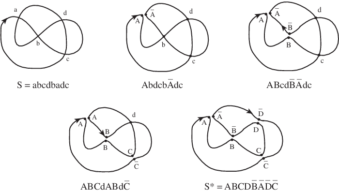The result of performing the splitting process on a closed plane curve is an embedded circle labeled by the split code. We will call this the split curve. To reconstruct the original curve from the split curve, we simply need to connect pairs of points $P$ and $\bar{P}$ by chords, and contract the chords to bring the points back together, as shown in Figure 4.

Figure 4: Expanding chords into crossings (reversing splits)

We can see from Figure 3 that these interiors of these chords will be disjoint from the split curve, so each chord lies entirely in the exterior or interior of the circle. Therefore, contracting the chord will bring together two arcs with (locally) opposite orientations, which means the corresponding labels of the split code must have opposite orientation. We conclude that if a crossing sequence is realizable, the two occurrences of each symbol in its split code must have opposite orientations.

Moreover, the chords will all be disjoint (we can see this in Figure 3 - the short chords required to join the pairs are all clearly non-intersecting). This leads us to look at the intersection graph of the split code.

Definition 2

The intersection graph $\Gamma(S)$ for a sequence S of length 2n, containing 2 occurrences each of n symbols, has one vertex for each symbol in S (we label the vertices of $\Gamma(S)$by the symbols of S). Vertices A and B in $\Gamma(S)$ are adjacent if and only if the symbols A and B alternate in S (so S contains either …A…B…A…B… or …B…A…B…A…).

The condition that the chords all be disjoint can be restated as requiring the intersection graph $\Gamma(S)$ to be bipartite (with one set of independent vertices corresponding to the chords inside the circle, and the other to the chords outside the circle). We can now state the main theorem of this section:

Theorem 1

[1] A crossing sequence S is realizable as the Gauss code of a closed curve in the plane if and only if the split sequence S* satisfies two conditions:

• The two occurrences of each symbol in S* have opposite orientations.

• The intersection graph $\Gamma(S^{*})$ is bipartite.

Proof: The discussion in this section shows that these conditions are both necessary; it remains to show that they are sufficient. Given a split curve satisfying the two conditions, we can construct a closed curve in the plane by connecting pairs of symbols with chords and expanding the chords into crossings, as in Figure 4. It only remains to check that this process will yield a single closed curve with Gauss code $S$ (this is the complete traceability of [7]).

Consider the construction process one chord at a time. We will add the chords between pairs of symbols in the reverse order from how they were split - i.e. the last symbol to be split is the first chord added. We can see from Figure 4 that the result of contracting this chord into a crossing is to reverse the orientation on the arc between the symbols. In other words, expanding the chord exactly reverses the splitting process of Definition 1. We can also see that, since the symbols had opposite orientations, the resulting curve still has one component. Continuing the process will therefore yield a closed curve with a single component whose Gauss code is the original crossing sequence $S$, as desired. $\Box$

Remarks: There are several remarks that should be made at this point.

1. Comparing with the D-switch operation of de Fraysseix and Ossona de Mendez [1], the condition that the two occurrences of a symbol have opposite orientation is equivalent to saying that a symbol and its twin are not adjacent in the interlacement graph. So, the result of Theorem 1 then also follows from the proof of Theorem 6 in [1].

2. Kauffman [4] provides another characterization, in which the first condition in Theorem 1 is replaced by the condition that the crossing sequence $S$ is evenly intersticed, meaning that between two occurrences of any symbol is a word of even length. However, Kauffman does not prove that this requirement is sufficient. It is not hard to show that, if $S$ is evenly intersticed, then the number of unsplit symbols between a pair of split symbols (at any stage in the process of splitting $S$) is even exactly when the split symbols have opposite orientations. Since, in $S^{*}$, the number of unsplit symbols is 0, and hence even, all pairs of split symbols have opposite orientations, so by Theorem 1 the crossing sequence is realizable. This shows that Kauffman’s characterization is also valid.

3. Not every sequence of symbols $S^{*}$ which satisfies the conditions of Theorem 1 is the split code of a crossing sequence. For example, if the reconstruction algorithm is applied to the sequence $AB\bar{A}\bar{B}$, the result will be a curve with two components; however, this is not a contradiction because this sequence cannot be obtained as the split code of a crossing sequence. To see this, observe that if we ”unsplit” symbol $B$ we are left with $AbAb$ - since the two occurrences of $A$ have the same orientation, this could not be the result of a splitting operation; attempting to unsplit $A$ leads to a similar situation.

4. The importance of Theorem 1 (and other such characterizations), is that it provides a polynomial-time algorithm for identifying Gauss codes, since there are known polynomial-time algorithms for identifying bipartite graphs.

3 Gauss Codes for Immersed Line Segments

Although a lot of work has been done on the realization problem for crossing sequences of closed curves in the plane, no-one seems to have considered the analogous problem for immersions of a line segment, or any other graph, in the plane. In this section we will build on the results for closed curves to develop a polynomial-time algorithm for determining whether a crossing sequence is realizable as the Gauss code for an immersed line segment.

As with closed curves, an immersion of the unit interval [0, 1] in the plane gives rise to a Gauss code by labeling the $n$ self-crossings and writing down the sequence of $2n$ labels. Unlike in Section 2, where Gauss codes were only well-defined modulo cyclic permutations, the Gauss code of an open curve has no indeterminacy. As in the last section we will look at the split code that results from splitting each crossing, as in Definition 1. As in the previous section, the splittings are chosen so that we always have a single curve. Unlike closed curves, the split code for an open curve may have some pairs of labels with the same orientation.

As in the last section, given the split code for a Gauss code, we can reconstruct the Gauss code by drawing an oriented line segment with $2n$ points labeled according to the split code, connecting pairs of points with the same label by disjoint chords and expanding the chords to crossings. The orientation of the line segment gives well-defined ”right” and ”left” sides. For closed curves the chords had to have both endpoints on the same side of the circle (since the chord could not cross the circle); for open curves, however, this is determined by whether the pair of symbols in the split code have the same or opposite orientations. If the pair has opposite orientations, then the corresponding chord must have both endpoints on the same side of the line segment; if the pair has the same orientation, then the chord must have endpoints on opposite sides of the line segment.

This leads to our first condition for a crossing sequence to be realizable as the Gauss code for an open curve.

Lemma 1

Let S be the Gauss code for an open curve, with split code S*. Say that A is a symbol in S* whose two occurrences have the same orientation. Then the occurrences of A cannot nest inside the occurrences of any other symbol in S*. In other words, we cannot have sequences $...B...A...A...B...$ or $...B...A...A...\bar{B}...$ inside S*.

Proof: Assume that the two occurrences of $A$ nest inside the occurrences of another symbol $B$. Then we have the situation shown in Figure 5.

Figure 5: $A$ nests inside $B$

The chord connecting the two occurrences of $A$, together with the line segment, divides the plane into two disjoint regions. One occurrence of $B$ is in one region, and the other occurrence of $B$ is in the other region - so it is impossible to connect them by a chord (regardless of the orientations of $B$) without crossing either the chord for $A$ or the line segment. So the split code S* could not arise from the Gauss code for an open curve, a contradiction. $\Box$

To find a complete characterization of realizable crossing sequences, we again turn to the intersection graph of the split code. However, for the case of open curves, we will use a directed intersection graph.

Definition 3

The intersection graph $\Gamma(S)$ for a sequence S of length 2n, containing 2 oriented occurrences each of n symbols, has one vertex for each symbol in S (we label the vertices of $\Gamma(S)$by the symbols of S). We say a vertex is fat if it is labeled by a symbol whose two occurrences in S have the same orientation; a thin vertex is labeled by a symbol whose two occurrences have opposite orientations. There is a directed edge from vertex A to vertex B in $\Gamma(S)$ if and only if S contains the sequence …A…B…A…B…. (ignoring orientations, so A and B may be either fat or thin). An example is shown in Figure 6.

Figure 6: Intersection graph for a split code, with fat and thin vertices

Moreover, a fat component of $\Gamma(S)$ is a connected component of the subgraph induced by the fat vertices. Similarly, a thin component is a connected component of the subgraph induced by the thin vertices.

Lemma 2

Let S be the Gauss code for an open curve, with split code S*. Then the thin vertices of $\Gamma(S^{*})$ can be colored using two colors (say red and blue) such that:

• Adjacent thin vertices have opposite colors (i.e. all the thin components of $\Gamma(S^{*})$ are bipartite).

• If thin vertices A and B both have directed edges to the same fat component F of $\Gamma(S^{*})$, then A and B have the same color.

• If thin vertices A and B both have directed edges from the same fat component F of $\Gamma(S^{*})$, then A and B have the same color.

• If A and B are thin vertices such that there is a directed edge from A to a fat component F of $\Gamma(S^{*})$ and a directed edge from F to B, then A and B have opposite colors.

Proof: These conditions all arise from the fact that, if $S$ is the Gauss code for an open curve, the curve can be reconstructed from $S^{*}$ by connecting each pair of symbols by disjoint chords. The chords corresponding to thin vertices of $\Gamma(S^{*})$ have both endpoints on the same side of the curve; those corresponding to fat vertices have endpoints on opposite sides. We color the thin vertices red if the corresponding chord has both endpoints on the right side of the curve, and blue if the endpoints are on the left side. Clearly, chords whose endpoints alternate must be on opposite sides in order to be disjoint, and so will have different colors, proving the first condition.

For the other conditions, we first observe that the chords corresponding to two fat vertices in the same fat component must begin and end on the same sides of the curve in order to be disjoint (see Figure 7).

Figure 7: Chords in the same fat component must be parallel to be disjoint

Say the chords in a fat component $F$ begin on the right side of the curve and end on the left side. Then any thin vertex with a directed edge to any vertex in $F$ corresponds to a chord on the left side of the curve. Similarly, any thin vertex with a directed edge from a vertex in $F$ corresponds to a chord on the right side of the curve (see Figure 8).

Figure 8: Chords for adjacent fat and thin vertices

Together, these observations show the last three conditions. $\Box$

These two lemmas suggest a method for reconstructing an immersion of an open curve from a crossing sequence (if possible), similar to the method in Section 2. First, check that the crossing sequence and its split sequence satisfy the conditions of Lemmas 1 and 2. Then use the split sequence to add chords to an embedded (oriented) line segment, and expand these chords (one at a time) into crossings as in Figure 9 (note that now the local orientations of the arcs may be the same or opposite).

Figure 9: Expanding chords into crossings (reversing splits)

The conditions of Lemmas 1 and 2 ensure that this can be done without introducing any undesired crossings. The next theorem shows that these conditions are sufficient for the Gauss code to be realizable.

Theorem 2

A Gauss code $G$ with split sequence $S$ is realizable as the Gauss code of an open curve in the plane if and only if $S$ satisfies the conditions of Lemmas 1 and 2.

Proof: As in Theorem 1, we need to show that the result of the reconstruction process is an immersed curve with one component and Gauss code $G$. Unlike the case of closed curves, the two occurrences of a symbol in $S$ may have the same orientation - in this case, expanding the chord does not preserve the number of components. However, if we expand the chords in the reverse order from how they were split (as we did in the proof of Theorem 1), then we will always be expanding a chord between two symbols with opposite orientations, and therefore preserving the number of components. This shows that the result of expanding all the chords is an immersed curve with one component and, since we’ve simply reversed the splitting process, with Gauss code $G$. $\Box$

Remark: Theorem 2 gives a polynomial time algorithm for recognizing a Gauss code, since all of the conditions of Lemmas 1 and 2 can be checked in polynomial time.

4 Gauss Codes for $\theta_{n}$-graphs

A $\theta_{n}$-graph is the graph consisting of two vertices and $n$ edges between these vertices. Figure 10 shows several examples.

Figure 10: Examples of $\theta_{n}$-graphs

In a sense, $\theta_{n}$-graphs are topologically the simplest graphs after $n$-cycles, so their spatial embeddings have been studied extensively [3, 5, 6]. This makes them a natural place to begin our development of Gauss codes for graphs.

For our purposes, we want to add a little more structure to the $\theta_{n}$-graphs. First of all, we will label the vertices $u$ and $v$ and give every edge an orientation so that it points from $u$ to $v$ (so the graph is directed). We will also fix a cyclic (counterclockwise) order of the edges around $u$ and $v$ (we say the graph is vertex-oriented). Figure 11 shows a $\theta_{3}$-graph with the additional structure indicated.

Figure 11: Example of a directed, vertex-oriented $\theta_{3}$-graph

Given an immersion of a $\theta_{n}$-graph in the plane (or sphere $S^{2}$) we can now define the Gauss code for the immersion as a set of $n$ sequences in some alphabet $A$ as follows. First, label each crossing in the immersion by an element of $A$ (distinct crossings receive distinct labels). Then we write out a sequence for each edge as we did for immersed circles in Section 2, writing the label for each crossing encountered as we follow the edge from $u$ to $v$. At the beginning and end of the sequence, place an integer between 0 and $n-1$ to indicate the position of the edge in the cyclic orders around the vertices $u$ and $v$, respectively. We end with a set of $n$ sequences, which are collectively the Gauss code for the immersion. An example of this is shown in Figure 12.

Figure 12: Example of a Gauss code from an immersed $\theta_{3}$-graph

More generally, we can consider any set of $n$ such sequences: sequences which begin and end with an integer between 0 and $n-1$ (each integer used once as a first symbol and once as a final symbol), and otherwise contain symbols from $A$ (with each symbol used twice in the set). We will generally refer to such sets of sequences as Gauss codes. The problem is to determine whether such a sequence can be realized as the Gauss code for an immersed $\theta_{n}$-graph (we call such codes realizable). Following the approach for classical Gauss codes, we will define a ”splitting” operation on the sequences, and look at the resulting ”split sequences”. The splitting operation is motivated by the idea of splitting the crossings of an immersed graph into two arcs. Since any crossing can be split in two different ways, we need to specify our choice. If an edge crosses itself, we will split the crossing so as to preserve the number of components of the graph (locally, the smoothed arcs will have opposite orientations); when two edges cross, we will split the crossing so as to preserve the orientations of the arcs. These operations are shown in Figure 13.

Figure 13: Splitting crossings

We can translate these operations into moves which can be performed directly on a Gauss code, regardless of whether or not the code is realizable. Given a Gauss code $G$ and a symbol $x$ used in the code, splitting G at x means:

• If there is a sequence $w=...x\alpha x...$ in $G$, replace it by $w^{*}=...X\alpha^{-1}\bar{X}...$, where $\alpha^{-1}$ is the result of writing the subsequence $\alpha$ in reverse order (reversing the orientation on any symbols which are already split), and leaving the rest of the sequence the same.

• If there are two sequences $w_{1}=\alpha x\beta$ and $w_{2}=\gamma x\delta$, replace them by $w_{1}^{*}=\alpha X\delta$ and $w_{2}^{*}=\gamma X\beta$.

A split sequence for G is the result of splitting $G$ at every symbol. Note that a given Gauss code may have many split sequences - the order in which the symbols are split will affect the final set of sequences. Observe that at every stage of the splitting process, the underlying graph is still a $\theta_{n}$-graph, with all edges directed from $u$ to $v$. Below is an example of transforming an abstract Gauss code for a $\theta_{3}$-graph into a split sequence (we use slashes to separate the codes for each edge):

$$u0abca1v/u1bc0v/u2cede2v\rightarrow u0Acb\bar{A}1v/u1bd0v/u2cede2v$$

$$\rightarrow u0AcBd0v/u1B\bar{A}1v/u2CEDE2v\rightarrow u0ACede2v/u1B\bar{A}1v/u2CBd0v$$

$$\rightarrow u0ACeD0v/u1B\bar{A}1v/u2CBDe2v\rightarrow u0ACE2v/u1B\bar{A}1v/u2CBDED0v$$

If a Gauss code is realizable, what can we say about its split sequence? In this case, we can imagine that the splittings truly were the result of splitting crossings as shown in Figure 13.

Lemma 3

Assume a Gauss code $G$ is realizable, and that $S$ is a split sequence for $G$. Let $w_{i}$ be the sequence in the set $S$ which begins with $i$ ($0\leq i\leq n-1$). Then:

1. The cyclic order of the sequences using the integer at the beginning is the reverse of the cyclic ordering using the integer at the end (modulo cyclic permutations).

2. If one occurrence of a symbol $X$ appears in $w_{i}$, then the second occurrence occurs in $w_{i-1}$, $w_{i}$ or $w_{i+1}$ (subscripts are computed modulo $n$).

3. If symbols $X$ and $Y$ both appear in the sequences $w_{i}$ and $w_{i+1}$, then they must appear in the same order in both sequences.

4. The symbols which appear in the sequence $w_{i}$ partition into 4 sets $A_{i-1,i}$, $A_{i,i+1}$, $B_{i}^{i-1}$ and $B_{i}^{i+1}$ such that

   • All symbols in $B_{i}^{j}$ appear twice in $w_{i}$, with opposite orientations.

   • If $X$ and $Y$ are both symbols in $B_{i}^{i-1}$ (respectively $B_{i}^{i+1}$), then $X$ and $Y$ do not interlace in $w_{i}$. I.e., $w_{i}$ does not have the form $...X...Y...\bar{X}...\bar{Y}...$.

   • All symbols in $A_{i-1,i}$ appear once in $w_{i}$ and once in $w_{i-1}$, with the same orientation.

   • All symbols in $A_{i,i+1}$ appear once in $w_{i}$ and once in $w_{i+1}$, with the same orientation.

   • No symbol in $A_{i-1,i}$ appears between two symbols in $B_{i}^{i-1}$.

   • No symbol in $A_{i,i+1}$ appears between two symbols in $B_{i}^{i+1}$.

Proof: The key idea is that, if $G$ is realizable, we can view $S$ as the result of splitting (in some order) all the crossings of an immersion of $\theta_{n}$ which realizes $G$. Since there are no more crossings after this splitting process is complete, the result will be an embedding of $\theta_{n}$ into the plane. Since there is essentially only one embedding of $\theta_{n}$ in the plane (to be precise, up to isotopy there is a unique spherical embedding), this means our split sequence can be viewed as the embedding shown in Figure 10, decorated by sequences of symbols along each edge. This gives the first condition of the lemma.

The original immersion of $\theta_{n}$ can be reconstructed by adding chords connecting the two occurrences of each symbol, and expanding those chords into crossings as shown in Figure 4, essentially reversing the splitting process. However, since these are all the crossings in the original immersions, the chords may not intersect each other or any of the edges of the embedded $\theta_{n}$. In particular, the two endpoints of the chord must lie on either the same edge or on (cyclically) neighboring edges, proving the second claim in the lemma. If two chords connect the same pair of edges, they must be non-intersecting, so their endpoints are in the same order along both edges, proving the third claim.

The fourth part of the lemma is also a consequence of the fact that no pair of chords may intersect, and that no chord can intersect the arcs of the embedded $\theta_{n}$. The chords with both endpoints on an edge $w_{i}$ must be partitioned into two sets - chords which lie in the region between $w_{i}$ and $w_{i-1}$ and those which lie in the region between $w_{i}$ and $w_{i+1}$. Each of these sets of chords must be non-intersecting. These are the sets $B_{i}^{i-1}$ and $B_{i}^{i+1}$ respectively. Moreover, in these cases the endpoints of the chord must be on the same side of the edge of the graph, so the labels must have opposite orientations. However, the chords between two adjacent edges must be on opposite sides of the two edges (on the right side of one edge and the left side of the other), so the labels will have the same orientation. The other conditions come from the fact that the chords in $B_{i}^{i-1}$ cannot intersect the chords between $w_{i}$ and $w_{i-1}$ (the elements of $A_{i-1,i}$), and similarly for $B_{i}^{i+1}$ and $A_{i,i+1}$. $\Box$

Lemma 3 suggests a method for reconstructing an immersion of $\theta_{n}$ from a Gauss code (if possible), as in the previous sections. First, compute a split sequence for the Gauss code. Then use the split sequence to add chords to the standard embedded $\theta_{n}$, and expand these chords into crossings as in Figure 9. The conditions of Lemma 3 ensure that this can be done without introducing any undesired crossings. All that remains is to check that the resulting diagram has the desired Gauss code.

Theorem 3

A Gauss code $G$ with split sequence $S$ is realizable as the Gauss code of an immersion of $\theta_{n}$ if and only if $S$ satisfies the conditions of Lemma 3.

Proof: As in Theorems 1 and 2, we need to show that the result of the reconstruction process is an immersed $\theta_{n}$ with Gauss code $G$. As before, we expand the chords between symbols in the reverse order that the symbols were split. In each case, we are either expanding a chord with endpoints of opposite orientations on the same edge, or a chord with endpoints of the same orientation on different edges. In both cases, we preserve the number of components of the immersion. Since these expansions exactly reverse the effects of the splitting process on the code, the resulting immersion of $\theta_{n}$ will have Gauss code $G$. $\Box$

Remark: Theorem 3 gives a polynomial time algorithm for recognizing a Gauss code, since all of the conditions of Lemma 3 can be checked in polynomial time. In particular, the partitioning into the sets $A_{i-1,i}$, $A_{i,i+1}$, $B_{i}^{i-1}$ and $B_{i}^{i+1}$ involves showing that the set of chords with both vertices on $w_{i}$ is bipartite, which can be done in polynomial time.

5 Gauss Codes for Graphs

We would like to extend the ideas of the last section to general graphs. Abstractly, a graph $G=(V,E)$ is a pair of a set $V$ of vertices and a set $E\subset V\times V$ of edges between pairs of vertices. We will allow loops (edges where both endpoints are the same) and multiple edges between two vertices. Our graphs will be directed, so each edge has an orientation. Finally, our graphs will also be vertex-oriented, meaning that we have a cyclic order on the edges incident to each vertex.

Given a graph $G$, a Gauss code for G consists of a set of symbols $A$ and a set of sequences in these symbols, one for each edge of the graph. Each sequence will begin with the vertex at the start of the edge, and the position of the edge in the cyclic ordering around that vertex, and end with the vertex at the end of the edge, with the position of the edge in the cyclic ordering around the end vertex. In between are symbols from $A$. Notice that the abstract graph $G$ can be reconstructed from the set of Gauss codes.

While an abstract graph has many possible Gauss codes, we can assign a unique code (up to cyclic permutation of the vertex orderings) to any immersion of the graph in the plane, just as we do for immersions of circles or $\theta_{n}$-graphs. In this case, the sequence of symbols just records the order of the crossings along each edge. An example is shown in Figure 14.

Figure 14: Example of a Gauss code from a graph immersion

We wish to address the problem of determining which Gauss codes for $G$ can be realized by an immersion of $G$ in the plane. We will assume that the initial graph $G$ is connected.

Our first observation is that every symbol in the set of sequences (other than the vertices) must appear exactly twice. This allows us to create a split code from the original Gauss code. As in the previous sections, the motivation for the split code is to split the crossings of an immersion of a graph in the plane. There are two ways to split a crossing (see Figure 2) - we want to perform the split so that the graph remains connected. If both splits preserve the connectedness of the graph, we can choose one arbitrarily. As before, we also want to keep track of the relative local orientations of the smoothed arcs. These operations can be defined abstractly in terms of the Gauss code. If $x$ is a symbol in the alphabet $A$, then splitting the code at $x$ means one of the following operations:

• If there is a sequence $w=\alpha x\beta x\gamma$, then the new sequence is $w^{*}=\alpha X\beta^{-1}\bar{X}\gamma$. So the subsequence $\beta$ has been reversed.

• If there are two sequences $w=\alpha x\beta$ and $u=\gamma x\delta$, then the new sequences are either $w^{*}=\alpha X\delta$ and $u^{*}=\gamma X\beta$ or $w^{*}=\alpha X\gamma^{-1}$ and $u^{*}=\delta^{-1}X\beta$. Notice that the underlying graph is changed in each case, but at least one of these graphs is connected. We will always make a choice which keeps the underlying graph connected.

The result of performing this splitting operation on every symbol in the set of sequences gives a split code for the original Gauss code. The splitting process is not unique - the final set of sequences after all crossings have been split will depend on the order in which they were split, and how they were split. Any of these possibilities is called a split code for the original Gauss code.

Lemma 4

If a Gauss code is derived from an immersion of a connected graph, then the underlying split graph for any split code is planar and connected; moreover, the split code determines a unique (up to isotopy) spherical embedding of the split graph.

Proof: If we begin with an immersion of a graph and split every crossing, we are left with a graph embedded in the plane; this implies that the graph underlying the split code is planar, and the split code is realized by some planar embedding. The embedding is connected since we choose our splittings to keep the graph connected. It remains to show that this embedding is unique (up to isotopy on the sphere).

We will describe an algorithm for constructing a planar embedding from the split code. We will show that (up to isotopy on the sphere) the algorithm produces at most one embedding, and that it fails to produce an embedding respecting the split code only if one does not exist. In fact, we will not use all the information of the split code, only the underlying graph and the order of the edges around each vertex. The idea of the algorithm is to trace out faces of the planar embedding.

Begin with an arbitrary vertex $v$, and an edge $e$ incident to $v$. Embed $v$ and $e$. Say that $w$ is the other endpoint of $e$. Let $f$ be the next edge adjacent to $w$ after $v$ (using the cyclic ordering of the edges adjacent to $w$), and add $f$ to the embedded graph. Continue this process, moving one edge around each vertex.

The first time we return to a vertex we have visited before, we will have two choices of how to draw the edge - clockwise or counterclockwise around the previously embedded parts of the graph. But these choices are isotopic on the sphere. Once this first choice is made, all future edges will connect two points on the boundary of a (topological) disk, so all possible ways to draw them will be isotopic. As a result, there are no more choices to be made, and the resulting embedding is unique.

When we come to an edge we have reached before, skip it and move to the next unused edge on that vertex. If there are no more unused edges on the vertex, then backtrack to the last vertex with an unused edge. Continue in this way until all the edges have been drawn (the procedure will terminate, since the graph is connected). If we are able to do this without edges crossing, we will have a planar embedding of the split graph, uniquely determined by the underlying graph and the vertex orientations. $\Box$

Lemma 4 allows us to embed the split code in the plane. As in earlier sections, if the original Gauss code is realizable then we can recover an immersion of a graph from this embedding code by connecting the two occurrences of each symbol in the split graph by disjoint chords which respect the orientations of the symbols, and then expanding the chords as in Figure 4. This leads us to the following theorem. The proof is very similar to that of Theorem 3 and is left to the reader.

Theorem 4

A Gauss code S for a graph G is realizable if and only if the paired symbols in the split graph S* can be connected by disjoint chords which respect the orientation of the symbols.

Question 1

Is there a polynomial time algorithm to determine whether a Gauss code for an arbitrary graph is realizable?

One approach to this problem is to follow what we have done for closed curves, open curves and $\theta$-graphs, and look at intersection graphs. There are at most two chords (up to isotopy) which can connect a pair of symbols in the split graph (respecting their orientation). We can look at the intersection graph of all these chords and rephrase Question 1 as follows.

Question 2

Given a graph with labeled vertices, where each label is used at most twice, is there a polynomial time algorithm for determining whether there is an independent set consisting of exactly one vertex with each label?

Remark: The difficulty arises when the split graph has cut edges. If both occurrences of a symbol appear on cut edges of the split graph, then there are two possible chords connecting them, and it is not clear how to choose one of these chords in polynomial time.

References

- [1] de Fraysseix, H. and Ossona de Mendez, P.: On a Characterization of Gauss Codes, Discrete Comput. Geom., v. 22, 1999, pp. 287-295
- [2] Dehn, M.: Über Kombinatorische Topologie, Acta Math. 67, 1936, pp. 123-168
- [3] Goda, H.: Bridge index for theta curves in the 3-sphere. Topology Appl., v. 79, 1997, pp. 177-196.
- [4] Kauffman, L.: Virtual Knot Theory, Europ. J. Combinatorics, v. 20, 1999, pp. 663-691
- [5] Kinoshita, S.: On -curves in and their constituent knots, Topology and computer science (Atami, 1986), Kinokuniya, Tokyo, 1987, pp. 211-216
- [6] Nikkuni, R.: Delta edge-homotopy on theta curves, Math. Proc. Cambridge Philos. Soc., v. 138, 2005, pp. 401-420.
- [7] Read, R.C. and Rosenstiehl, P.: On the Gauss Crossing Problem, Colloq. Math. Soc. Janos Bolyai, v. 18, Combinatorics, Keszthely, Hungary, 1976, pp. 843-876