Numerical verification of a gap condition for linearized NLS

Abstract

We make a detailed numerical study of the spectrum of two Schrödinger operators $L_{\pm}$ arising in the linearization of the supercritical nonlinear Schrödinger equation (NLS) about the standing wave, in three dimensions. This study was motivated by a recent result of the second author on conditional asymptotic stability of solitary waves in the case of a cubic nonlinearity. Underlying the validity of this result is a spectral condition on the operators $L_{\pm}$, namely that they have no eigenvalues nor resonances in the gap (a region of the positive real axis between zero and the continuous spectrum,) which we call the gap property. The present numerical study verifies this spectral condition, and further shows that the gap property holds for NLS exponents of the form $2\beta+1$, as long as $\beta_{*}<\beta\leq 1$, where

$$\beta_{*}=0.913958905\pm 1e-8.$$

Our strategy consists of rewriting the original eigenvalue problem via the Birman-Schwinger method. From a numerical analysis viewpoint, our main contribution is an efficient quadrature rule for the kernel $1/|x-y|$ in ${\mathbb{R}}^{3}$, i.e., provably spectrally accurate. As a result, we are able to give similar accuracy estimates for all our eigenvalue computations. We also propose an improvement of the Petviashvili’s iteration for the computation of standing wave profiles which automatically chooses the radial solution.

All our numerical experiments are reproducible. The Matlab code can be downloaded from

http://www.acm.caltech.edu/~demanet/NLS/

1 Introduction

Suppose that $\psi(t,x)=e^{it\alpha^{2}}\phi(x)$ with $\alpha\neq 0$ and $x\in{\mathbb{R}}^{d}$ is a standing wave solution of the NLS

$$i\partial_{t}\psi+\Delta\psi+|\psi|^{2\beta}\psi=0,$$ (1)

where $0<\beta<\frac{2}{d-2}$ if $d\geq 3$ and $0<\beta<\infty$ if $d=1,2$. Here we assume that $\phi=\phi(\cdot,\alpha)$ is a ground state, i.e.,

$$\alpha^{2}\phi-\Delta\phi=\phi^{2\beta+1},\qquad\phi>0.$$

It is known that such $\phi$ exist and that they are radial, smooth, and exponentially decaying, see Berestycki, Lions [BerLio] and for uniqueness, Kwong [Kwo]. In one dimension $d=1$, these ground states are explicitly given as

$$\phi(x)=\frac{(\beta+1)^{\frac{1}{2\beta}}}{\cosh^{\frac{1}{\beta}}(\beta x)}$$ (2)

when $\alpha=1$ (for other values of $\alpha\neq 0$ rescale), but in higher dimensions no explicit expression is known. From now on, we shall assume that $d=3$.

A much studied question is the stability of these standing waves, both in the orbital (or Lyapunov) sense and the asymptotic sense. For the former, see for example Grillakis, Shatah, Strauss [GriShaStr1], [GriShaStr2], Weinstein [Wei1], [Wei2], Grillakis [Gri], and for the latter, Buslaev, Perelman [BusPer1], Cuccagna [Cuc]. Reviews are in Strauss [Str] and Sulem, Sulem [SulSul].

In order to study stability, one generally linearizes around the standing wave. This process leads to matrix Schrödinger operators of the form

$${\mathcal{H}}={\mathcal{H}}_{0}+V=\left[\begin{array}[]{cc}-\Delta+\alpha^{2}&0\\ 0&\Delta-\alpha^{2}\end{array}\right]+\left[\begin{array}[]{cc}-V_{1}&-V_{2}\\ V_{2}&V_{1}\end{array}\right]$$

on $L^{2}({\mathbb{R}}^{d})\times L^{2}({\mathbb{R}}^{d})$. Here, $V_{1}=(\beta+1)\phi^{2\beta}$ and $V_{2}=\beta\phi^{2\beta}$.

Conjugating ${\mathcal{H}}$ by the matrix $\left[\begin{array}[]{cc}1&i\\ 1&-i\end{array}\right]$ leads to the matrix operator

$$\left[\begin{array}[]{cc}0&iL_{-}\\ -iL_{+}&0\end{array}\right]$$

with

$$L_{-} =-\triangle+\alpha^{2}-\phi^{2\beta}$$

$$L_{+} =-\triangle+\alpha^{2}-(2\beta+1)\phi^{2\beta}$$

The continuous spectrum of both $L_{-}$ and $L_{+}$ equals $[\alpha^{2},\infty)$. Since $L_{-}\phi=0$ and $\phi>0$, it follows that zero is a simple eigenvalue and the bottom of the spectrum of $L_{-}$. Moreover, $L_{+}\partial_{j}\phi=0$ for $1\leq j\leq 3$ so that ${\rm ker}(L_{+})\subset\{\partial_{j}\phi\>:\>1\leq j\leq 3\}$. In fact, for monomial nonlinearities it is known that there is equality here, see Weinstein [Wei2], and that there is a unique negative bound state of $L_{+}$.

It is known that $L_{-}\geq 0$ implies that the spectrum ${\rm spec}({\mathcal{H}})$ satisfies ${\rm spec}({\mathcal{H}})\subset{\mathbb{R}}\cup i{\mathbb{R}}$ and that all points of the discrete spectrum other than zero are eigenvalues whose geometric and algebraic multiplicities coincide. On the other hand, the zero eigenvalue of ${\mathcal{H}}$ has geometric multiplicity four and algebraic multiplicity eight provided $\beta\neq\frac{2}{3}$, whereas for the $L^{2}$-critical case $\beta=\frac{2}{3}$ the algebraic multiplicity increases to ten. For this see [Wei1], [BusPer1] or [RodSchSof1], [ErdSch].

In order to carry out a meaningful asymptotic stability analysis it is essential to understand the discrete spectrum of ${\mathcal{H}}$. The root space at zero was completely described by Weinstein [Wei2]. Moreover, it is also well-known that

$${\rm spec}({\mathcal{H}})\subset{\mathbb{R}}\text{\ \ iff\ \ }\beta\leq\frac{2}{3}$$

whereas in the range $\frac{2}{3}<\beta<2$ there is a unique pair of simple complex-conjugate eigenvalues $\pm i\gamma$. This latter property reflects itself in the nonlinear theory in the following way: Orbital stability holds iff $\beta<\frac{2}{3}$, see Berestycki, Cazenave [BerCaz], Weinstein [Wei2], Cazenave, Lions [CazLio], and [GriShaStr1], [GriShaStr2].

In [Sch] the second author investigated conditional asymptotic stability for the unstable case $\beta=1$. This analysis depended on the fact that zero is the only eigenvalue of ${\mathcal{H}}$ in the interval $[-\alpha^{2},\alpha^{2}]$ and that the edges $\pm\alpha^{2}$ are not resonances. The fact that $\pm\alpha^{2}$ are neither eigenvalues nor resonances is the same as requiring that the resolvent $({\mathcal{H}}-z)^{-1}$ remains bounded on suitable weighted $L^{2}({\mathbb{R}}^{3})$ spaces for $z$ close to $\pm\alpha^{2}$.

Using some ideas of Perelman [Per2], it is shown in [Sch] that these properties can be deduced from the following properties of $L_{+},L_{-}$: Neither $L_{+}$ nor $L_{-}$ have any eigenvalues in the gap $(0,\alpha^{2}]$ and $L_{-}$ has no resonance at $\alpha^{2}$.

In one dimension $d=1$, the spectral properties of $L_{-}$ and $L_{+}$ can be determined completely since the generalized eigenfunctions of these operators (more precisely, the Jost solutions) can be given explicitly in terms of certain hypergeometric functions, see Flügge [Flu], Problem 39 on page 94. This is due to the special form of the ground state (2).

Unfortunately, it seems impossible to determine similar properties for the case of three dimensions by means of purely analytical methods. We therefore verify this gap property of $L_{\pm}$ numerically via the Birman-Schwinger method. We will refer to the gap property as the fact that $L_{\pm}$ have no eigenvalues in $(0,\alpha^{2}]$ and no resonance at $\alpha^{2}$. Our main result is as follows.

Claim 1.

There exists a number $\beta_{*}=.913958905\pm 1e-8$ so that for all $\beta_{*}<\beta\leq 1$ the gap property holds.

This statement can also be continued beyond $\beta=1$. We only went up to $1$ since $\beta=1$ alone is needed in [Sch]. In the range $\beta<\beta_{*}$, our numerical analysis shows that the operator $L_{+}$ has eigenvalues in the gap $(0,1]$. This is perhaps surprising, since it shows that the gap property does not hold for the entire $L^{2}({\mathbb{R}}^{3})$ super-critical range $\frac{2}{3}<\beta<2$. However, it does hold at $\beta=1$. In particular, the method of proof from [Sch] does not apply to all $\beta>\frac{2}{3}$ since it relies on the gap property. In contrast, in one dimension $d=1$, Krieger and the second author showed that this method does apply to the entire super-critical range $\beta>2$. In fact, there, the gap property does hold for all $\beta>1$, see [Flu].

In the remainder of this paper, we will be concerned with the description of the numerical method, and will study its convergence properties. Note that we did not formulate our main result as a theorem because the error bound we give on $\beta_{*}$ is based on numerical observations of convergence of the method. A fully rigorous justification would involve either an a priori estimate for this bound, or a provably reliable a posteriori estimate. For this, we would probably need to (1) derive quantitative estimates of regularity and decay for $\phi(x)$ and other functions, with explicit values of the constants, and (2) give a full treatment of the propagation of round-off errors from a countless number of sources. This type of heroic exercise would contribute little to the understanding of the accuracy of the numerical method, so we chose to spare the reader.

2 Description of the numerical method

2.1 The Birman-Schwinger method

A direct numerical computation of the eigenvalues of $L_{\pm}$ would be problematic near $\alpha^{2}$, the edge of the continuous spectrum. For example, it is unclear if a perceived numerical eigenvalue at $0.99\,\alpha^{2}$ belongs to the gap or if it has escaped from the continuous spectrum. Decay of the corresponding eigenfunction might help in making a decision, but this criterion is unacceptable over a truncated computational domain. Instead, we will reformulate the problem by the Birman-Schwinger method, which we now recall.

Let $H=-\triangle-V$, where $V>0$ is a bounded potential that decays at infinity. In our case, this is $H=L_{\pm}-\alpha^{2}I$. We would like to filter out positive eigenvalues, so assume $Hf=-\lambda^{2}f$ where $\lambda>0$ and $f\in L^{2}$. Then $g=Uf$, where $U=\sqrt{V}$ satisfies

$$g=U(-\triangle+\lambda^{2})^{-1}Ug.$$

In other words, $g\in L^{2}$ is an eigenfunction of

$$K(\lambda)=U(-\triangle+\lambda^{2})^{-1}U$$

with eigenvalue one. Note that $K(\lambda)$ is a compact, positive operator. Conversely, if $g\in L^{2}$ satisfies $K(\lambda)g=g$, then

$$f:=U^{-1}g=(-\triangle+\lambda^{2})^{-1}Ug\in L^{2}$$

and $Hf=-\lambda^{2}f$. Moreover, the eigenvalues of $K(\lambda)$ are strictly increasing as $\lambda\to 0$. Hence, we conclude that

$$\#\Big\{\lambda\>:\>{\rm ker}(H-\lambda^{2})\neq\{0\}\Big\}=\#\Big\{E>1\>:\>{\rm ker}(K(0)-E)\neq\{0\}\Big\}\;,$$

counted with multiplicity.

Finally, in view of the symmetric resolvent identity, viz.

$$(H-z)^{-1}=(-\triangle-z)^{-1}+(-\triangle-z)^{-1}U\Big[I-U(-\triangle-z)^{-1}U\Big]^{-1}U(-\triangle-z)^{-1}.$$

This shows that the Laurent expansion of $(H-z)^{-1}$ around $z=0$ does not involve negative powers of $z$ iff $I+U(-\triangle-z)^{-1}U$ is invertible at $z=0$ which is the same as requiring that

$${\rm ker}\{I-U(-\triangle)^{-1}U\}=\{0\}$$

because of the Fredholm alternative (assuming that $V$ decays sufficiently fast at infinity to insure compactness). In other words, if $H$ has no resonance or eigenvalue at the origin, then $K(0)$ will not show an eigenvalue $E=1$, and conversely.

Let us count the eigenvalues $\{\lambda_{j}\}_{j=1}^{\infty}$ of $K(0)=U(-\triangle)^{-1}U$ (which are all non-negative) in decreasing order. Then we arrive at the following conclusion: Let $N$ be a positive integer. Then the operator $H$ has exactly $N$ negative eigenvalues and neither an eigenvalue nor a resonance at zero iff $\lambda_{1}\geq\ldots\geq\lambda_{N}>1$ and $\lambda_{N+1}<1$.

Note that spectrum of the self-adjoint, compact Birman-Schwinger operator $K(0)$ is discrete and robust to numerical perturbations near $E=1$, which is the desired numerical effect. Since $K(0)$ is compact, eigenvalues cannot accumulate to $E=1$ from below, and are in no way related to the continuous spectrum of $H$.

In view of the preceding, we therefore need to show the following to justify [Sch]: For $\beta=1$, the second largest eigenvalue of

$$K_{-}(x,y)=\frac{\phi^{\beta}(x)\phi^{\beta}(y)}{4\pi|x-y|}$$

is below one, and the fifth largest eigenvalue of

$$K_{+}(x,y)=(2\beta+1)\frac{\phi^{\beta}(x)\phi^{\beta}(y)}{4\pi|x-y|}$$

is below one. These properties will then imply the gap property, i.e., $L_{\pm}$ have no eigenvalues in $(0,1]$ and no resonance at $1$.

2.2 The modified Petviashvili’s iteration

The first step of the numerical method is to find the soliton $\phi(x)$, which is the unique positive, radial, decaying solution of

$$-\Delta\phi+\phi=\phi^{2\beta+1},$$ (3)

unique up to translation. As mentioned earlier, $\phi(x)$ is in fact exponentially decaying. A naive approach would be to solve a descent equation like

$$\frac{\partial u}{\partial t}=\Delta u-u+|u|^{2\beta}u,$$

but, as shown in [BerLioPel], this equation is unstable near the fixed manifold of interest. Instead, we will solve the modified Petviashvili’s iteration which reads

$$\phi_{n+1}=M_{n}^{\gamma}(I-\Delta)^{-1}(|\phi_{n}|^{2\beta}\phi_{n})+\delta\sum_{j=1}^{3}R_{n,j}\frac{\partial\phi_{n}}{\partial x_{j}}$$ (4)

The initial guess $\phi_{0}$ can for example be taken as a Gaussian. The choice of constants $M_{n},R_{n,j},\gamma$ and $\delta$ is crucial for convergence of the iteration, and is given by

$$M_{n} =\frac{\int(1+|\xi|^{2})(\widehat{\phi_{n}})^{2}\,d\xi}{\int\widehat{\phi_{n}}\,\widehat{(|\phi_{n}|^{2\beta}\phi_{n})}\,d\xi},$$ (5)

$$R_{n,j} =\frac{\int(1+|\xi|^{2})\widehat{\phi_{n}}\,\widehat{\partial_{j}\phi_{n}}\,d\xi}{\int\widehat{\partial_{j}\phi_{n}}\,[\partial_{j}(|\phi_{n}|^{2\beta}\phi_{n})]^{\wedge}\,d\xi},$$ (6)

$$\gamma =\frac{2\beta+1}{2\beta},$$ (7)

$$\delta =-1/2,$$ (8)

where $\partial_{j}=\frac{\partial}{\partial x_{j}}$, and the hat denoting Fourier transformations. This iteration, without the second term, was introduced by Petviashvili in 1976, and convergence was proved recently in [PelSte]. The addition of the second term is a minor increment whose purpose is to fix a potential source of instability due to numerical discretization and to force the iteration to choose the radial soliton (centered at the origin). This will be explained and justified in section 3.

Numerically, $(I-\Delta)^{-1}$ is realized in the Fourier domain, and Fourier transformations are implemented via the Fast Fourier Transform (FFT). Discretization issues are addressed in the next section. In practice, the iteration is accelerated via Aitken’s method applied pointwise, i.e.,

$$\phi^{A}_{n}(x)=\phi_{n}(x)-\frac{(\phi_{n+1}(x)-\phi_{n}(x))^{2}}{\phi_{n+2}(x)-2\phi_{n+1}(x)+\phi_{n}(x)}.$$

The iteration is stopped when the Euler-Lagrange equation (3) is satisfied up to some very small tolerance $\tau$ in $L^{2}$. The resulting approximation of the soliton will be denoted by $\tilde{\phi}$.

2.3 Truncation and Discretization

We now take up the task of computing the eigenvalues of the Birman-Schwinger operators as defined in Section 2.1. The first step is to truncate the three-dimensional computational domain to a cube of sidelength $L$ centered at the origin and to discretize functions $f(x)$ by evaluating them on the regular grid

$$x_{j}=(j_{1},j_{2},j_{3})\frac{L}{N},$$ (9)

with $j_{1},j_{2},j_{3}$ integers obeying $-N/2\leq j_{k}\leq N/2-1$. Operators are, in turn, discretized as matrices acting on ‘vectors’ of function samples $f(x_{j})$. Tools of numerical linear algebra can then be invoked to compute the eigenvalues of these matrices.

Typical values of $L$ and $N$ for which discretizing $K_{\pm}$ is expected to be reasonably accurate are $L\simeq 20$ and $N\simeq 100$. In this context, several vectors of $N^{3}\simeq 10^{6}$ function samples can comfortably be stored simultaneously in the memory of a 2005-era computer, but we cannot yet afford to manipulate matrices containing $N^{6}\simeq 10^{12}$ elements. This rules out the possibility of using popular approaches such as the QR algorithm, which compute eigenvalues by operating directly on the matrix entries.

Instead, we will resort to a modification of the power method, known as the implicitly restarted Arnoldi iteration, which is implemented in Matlab’s eigs command [Eigs]. This method has the advantage of only requiring applications of the operator to diagonalize, i.e., matrix-vector products. For well-conditioned problems, such as the one we are addressing, eigs computes the top eigenvalues of the finite matrix up to machine precision, i.e., about 15 decimal digits in Matlab.

The only remaining issue is then to find a good discretization $\tilde{K}_{\pm}$ of the Birman-Schwinger operators $K_{\pm}$, and to quantify the accuracy. Multiplication by $\phi(x)$ to some power will be done sample-wise on the grid $x_{j}$. Inverting minus the Laplacian in a space of decaying functions over $\mathbb{R}^{3}$, or equivalently convolving with the fundamental solution $G(x)=\frac{1}{4\pi|x|}$, is a bit more complicated. Discretizing $G(x)$ by sampling at $x_{j}$ is quite inaccurate and is problematic if $x=0$ belongs to the grid $x_{j}$. Dividing by $|\xi|^{2}$ in frequency poses similar difficulties. Instead, for reasons which will be explained in Section 3, we use the following discretization,

$$\tilde{G}(x_{j})=\left\{\begin{aligned} \frac{1}{2\pi^{2}|x_{j}|}\left(\frac{L}{N}\right)^{3}\,\text{Si}(\frac{\pi N|x_{j}|}{L})\qquad&\text{if }x_{j}\neq 0,\\ \frac{1}{2\pi}\left(\frac{L}{N}\right)^{2}\qquad&\text{if }x_{j}=0,\end{aligned}\right.$$ (10)

where $\text{Si}(x)=\int_{0}^{x}\frac{\sin t}{t}\,dt$. The discrete (circular) convolution of $\tilde{G}(x_{j})$ with a vector $f(x_{j})$ is computed efficiently as the multiplication $\widehat{\tilde{G}(x_{j})}\,\widehat{f(x_{j})}$ of their respective FFT, followed by an inverse FFT.

In this context, applying the full Birman-Schwinger operator, say $K_{-}$, to a vector of samples $f(x_{j})$ consists of the obvious sequence of steps: (1) multiply $f(x_{j})$ by $\tilde{U}(x_{j})=\tilde{\phi}(x_{j})^{\beta}$, (2) perform an FFT, (3) multiply the result by $\widehat{\tilde{G}(x_{j})}$, (4) perform an inverse FFT, and finally (5) multiply the result by $\tilde{U}(x_{j})$ again.

Since the complexity of a one-dimensional FFT in Matlab is $O(N\log N)$ operations for most values of $N$ (not necessarily a power of two), one application of $\tilde{K}_{\pm}$ will require $O(N^{3}\log N)$ operations. This is a substantial improvement over the naive matrix-vector product which would require $O(N^{6})$ operations.

3 Convergence analysis

3.1 The modified Petviashvili’s iteration

In this section we discuss convergence of the iteration (4). The first result in this direction, in the case $\delta=0$, can be found in ref. [PelSte]. To make this discussion self-contained, we recall their argument and apply it to our specific problem.

Theorem 2.

(Pelinovsky, Stepanyants.) Let $\phi(x)$ be the unique radial solution of (3) and $H^{1}_{r}({\mathbb{R}}^{3})$ denote the subset of all radial functions in $H^{1}({\mathbb{R}}^{3})$. Consider the iteration (4) with $M_{n}$ and $\gamma$ given by equations (5), but $\delta=0$. Then there exists an open neighborhood $\mathcal{N}$ of $\phi$ in $H^{1}_{r}({\mathbb{R}}^{3})$, in which $\phi$ is the unique fixed point and (4) converges to $\phi$. The iteration is strictly stable in the sense that, for all $\phi_{0}\in\mathcal{N}$,

$$||\phi_{n+1}-\phi||_{1}\leq(1-C)||\phi_{n}-\phi||_{1},\qquad 0<C\leq 1,$$ (11)

where $||\cdot||_{1}$ is the norm in the Sobolev space $H^{1}({\mathbb{R}}^{3})$.

Proof.

Put $p=2\beta+1$. Let us first write down the linearized iteration, about the fixed point $\phi$, for the perturbation $w_{n}=\phi_{n}-\phi$. It reads

$$\hat{w}_{n+1}=(1-p)\gamma a_{n}\hat{\phi}+p\frac{\widehat{\phi^{p-1}}*\hat{w}_{n}}{1+|\xi|^{2}},$$ (12)

where $*$ denotes convolution, $a_{n}$ comes from the linearization of $M_{n}$, and is given by

$$a_{n}=\frac{\int w_{n}\phi^{p}}{\int\phi^{p+1}}.$$

(Up to higher-order terms, we have the asymptotic relation $1+(1-p)a_{n}\sim M_{n}$.) This formula suggests that $\phi$ plays a special role for the stability of the linearized iteration. Indeed, we claim that we can actually expand $w_{n}$ as

$$w_{n}=a_{n}\phi+q_{n},$$ (13)

where $a_{n}$ is exactly as defined above, and $q_{n}$ is a remainder. In order to see this, let us introduce the operator $A=(I-\Delta)^{-1}\mathcal{H}$, where $\mathcal{H}=I-\Delta-p\phi^{p-1}$. It is easy to check that is it bounded and self-adjoint with respect to the $H^{1}$ inner product,

$$(f,g)\equiv\langle f,(I-\Delta)g\rangle.$$

The operator $A$ therefore provides a spectral decomposition of $L^{2}({\mathbb{R}})$, orthogonal with respect to the inner product $(\cdot,\cdot)$. It was noticed in [PelSte], (or by a straightforward extension of their argument,) that the spectra of $A$ and $\mathcal{H}$ obey

$$\mbox{dim}(\mbox{neg}(A)) =\mbox{dim}(\mbox{neg}(\mathcal{H}))=1,$$

$$\mbox{null}(A) =\mbox{null}(\mathcal{H})=3.$$

The first four eigenfunctions of $A$ are precisely $\phi$ and $\partial_{i}\phi$, with eigenvalues $1-p<0$ and $0$ respectively. Equation (13) is just the expansion of $w_{n}$ in this orthogonal system. Since the iterates $\phi_{n}$ are all radial, the components along $\partial_{i}\phi$ are zero. The remainder $q_{n}$ belongs to the space $Y_{p}$ defined by

$$Y_{p}=\{u\in L^{2}({\mathbb{R}}^{3}):\langle u,\phi^{p}\rangle=\langle u,\partial_{i}\phi^{p}\rangle=0\}.$$

In the space $Y_{p}$, the spectrum of $A$ is strictly positive, bounded from below by the fifth eigenvalue $\lambda_{5}>0$ and from above by

$$\lambda_{M}=\sup_{u}\frac{(u,Au)}{(u,u)}=1-p\,\inf_{u}\frac{\langle u,\phi^{p-1}u\rangle}{(u,u)}=1.$$

For the last equality we have used the fact that $\phi(x)>0$ and $\phi(x)\to 0$ as $|x|\to\infty$.

The recurrence equations for $a_{n}$ and $q_{n}$ can be found from equation (12),

$$a_{n+1} =(p-\gamma(p-1))a_{n},$$

$$q_{n+1} =(I-A)q_{n}.$$

The choice we made for $\gamma$ ensures that the component along $\phi$ is immediately put to zero (in the linearized iteration.) It is also clear that we have $||q_{n+1}||_{1}\leq(1-\lambda_{5})||q_{n}||_{1}$ in $H^{1}({\mathbb{R}}^{3})$. In the scope of the linearized iteration, equation (11) follows with $C=\lambda_{5}$.

Call $\mathcal{P}$ the nonlinear operator for the Petviashvili iteration in the case $\delta=0$, so that (4) is written as $\phi_{n+1}=\mathcal{P}(\phi_{n})$. We follow [PelSte] and apply the contraction mapping theorem in a neighborhood of the pixed point $\phi$, within the closed subspace $H^{1}_{r}({\mathbb{R}}^{3})$. We have already computed the Fréchet derivative of $\mathcal{P}$ at $\phi$,

$$\mathcal{P}^{\prime}(\phi)w=(I-A)P_{Y_{p}}w,$$ (14)

where $P_{Y_{p}}$ is the projection onto $Y_{p}$, orthogonal in $H^{1}$. Let $0<\epsilon<\lambda_{5}$. By continuity of $\mathcal{P}^{\prime}(u)$ as a function of $u$, in the operator $H^{1}$ norm, we can assert that there exists a small open neighborhood $\mathcal{N}$ of $\phi$ in which

$$||\mathcal{P}^{\prime}(u)||_{1\to 1}<1-\lambda_{5}+\epsilon.$$

By a standard application of the contraction mapping theorem (see [HutPym] p.126), the fixed point is unique in $\mathcal{N}$ and we have the estimate

$$||\phi_{n+1}-\phi||_{1}\leq(1-\lambda_{5}+\epsilon)||\phi_{n}-\phi||_{1}.$$

This concludes the proof. ∎

Let us now examine how the above argument generalizes to the case $\delta\neq 0$. The purpose of the second term in equation (4) is precisely to put to zero the components along the three basis functions $\partial_{i}\phi$, should the initial condition not be radial. This is also useful in the context of the numerical realization of $\mathcal{P}$, since numerical round-off errors do not correspond in general to radial perturbations. To be precise, the linearized iteration (12) becomes

$$\hat{w}_{n+1}=(1-p)\gamma a_{n}\hat{\phi}+2\delta\sum_{j=1,2,3}b_{n,j}\widehat{\partial_{j}\phi}+p\frac{\widehat{\phi^{p-1}}*\hat{w}_{n}}{1+|\xi|^{2}},$$

with $a_{n}$ as previously and

$$b_{n,i}=\frac{\int w_{n}\partial_{i}\phi^{p}}{\int\partial_{i}\phi\partial_{i}\phi^{p}}$$

is the component of $w_{n}$ along $\partial_{i}\phi$, in the natural $H^{1}$ inner product. So we have

$$w_{n}=a_{n}\phi+\sum_{j}b_{n,j}\partial_{j}\phi+q_{n},$$

and the recurrence relation for $b_{n,i}$ is

$$b_{n+1,i}=(1+2\delta)b_{n,i}.$$

Choosing $\delta=-1/2$ as advocated previously will put to zero the components along $\partial_{i}\phi$.

In practice the modification $\delta=-1/2$ works very well, see section 4. The analysis of the linearized iteration does not pose any difficulty. However, we have been unable to extend the argument of theorem 2 to the full nonlinear iteration. The operator $\mathcal{P}$ is in general not defined on $H^{1}$, because the constants $R_{n,i}$ involve 3/2 derivatives of $\phi_{n}$ in $L^{2}$. A fortiori, $\mathcal{P}$ is not Frechet-differentiable for functions in $H^{1}$. Note that the contraction argument cannot work, since the soliton $\phi$ is not unique in $H^{1}({\mathbb{R}}^{3})$ – it is unique up to a translation. The question of stability of the modified Petviashvili’s iteration in the non-radial case is possibly related to the problem of proving uniqueness of the radial soliton, which, in itself, is not trivial.

3.2 Truncation and Discretization

In this section we prove spectral convergence of the proposed discretization of the Birman-Schwinger operator, which is numerical analysis jargon for (almost) exponential convergence with respect to the large discretization parameters $L$ and $N/L$. Recall that we denote by $x_{j}=(j_{1},j_{2},j_{3})\frac{L}{N}$, $j\in{\mathbb{Z}}^{3}$, the nodes of a cubic grid with spacing $L/N$ in all three directions, not necessarily bounded in some of the arguments that follow. Obviously, we take $L\leq N$. Unless otherwise specified, we are considering the operator $K_{-}$, since $K_{+}=(2\beta+1)K_{-}$.

We now formulate our main result. Most of the rest of this section is devoted to its justification. We will use the notation $\langle x\rangle=\sqrt{1+|x|^{2}}$.

Theorem 3.

Let $K$ be the Birman-Schwinger operator as above, and $\tilde{K}$ its numerical realization, extended to functions of continuous $x$ by sampling and interpolation (see below for details). Let $\delta>0$ be the decay rate of $U(x)=\phi(x)^{\beta}$, $|U(x)|\leq C\cdot e^{-\delta|x|}$. Assume that Petviashvili’s method gives an accurate approximation $\tilde{\phi}$ of the soliton in the sense that, for some $\epsilon>0$, and denoting $\tilde{U}=\tilde{\phi}^{\beta}$,

$$|U(x_{j})-\tilde{U}(x_{j})|\leq C\cdot\min(\frac{\epsilon}{\langle x_{j}\rangle},e^{-\delta|x_{j}|}).$$ (15)

Then we have, for all $s>3/2$ and $f\in H^{s}({\mathbb{R}}^{3})$, in exact arithmetic,

$$||(K-\tilde{K})f||_{L^{2}}\leq C_{s}\cdot\left[\epsilon+Le^{-\delta L/4}+\left(\frac{N}{L}\right)^{-s}\right]\cdot||f||_{H^{s}},$$ (16)

for some constant $C_{s}>0$ depending on $s$.

Discretization is error-free in the context of the Shannon sampling theorem. Let us introduce $B_{N/L}({\mathbb{R}}^{3})$, the space of band-limited square-integrable functions,

$$B_{N/L}({\mathbb{R}}^{3})=\{u\in L^{2}({\mathbb{R}}^{3}):\hat{u}(\xi)=0,\;|\xi|>\pi N/L\}.$$

The hat denotes Fourier transformation. We can then define the sampling operator $S$, and interpolation operator $T$, as

$$S:B_{N/L}\to\ell^{2},\quad f(x)\mapsto\{f(x_{j})\}.$$

$$T:\ell^{2}\to B_{N/L},\quad\{f(x_{j})\}\mapsto\sum_{j\in{\mathbb{Z}}^{3}}h(x-x_{j})f(x_{j}).$$

Here $h(x)$ is the interpolating kernel defined by $\hat{h}(\xi)=\left(\frac{L}{N}\right)^{3}$ if $|\xi|\leq\frac{\pi N}{L}$, and zero otherwise. The content of Shannon’s sampling theory is that $S$ is an isometry from $B_{N/L}$ to $\ell^{2}$, and $T$ is in that context both the adjoint and a left inverse for $S$ on its range (hence the interpolation property of $h$.) Note that the properly normalized $\ell^{2}$ norm is

$$\|\{f(x_{j})\}_{j}\|_{\ell^{2}}=\sqrt{\left(\frac{L}{N}\right)^{3}\sum_{j}|f(x_{j})|^{2}}$$

With a slight abuse of notations, let us denote by $\tilde{G}$ the operator of discrete convolution by $\tilde{G}(x_{j})$, defined in equation (10). This particular expression for the weights $\tilde{G}(x_{j})$ is chosen so that the inversion of the Laplacian is exact on decaying band-limited functions. By ‘decaying’, we mean a member of some weighted $L^{2}$ space. More generally, let us introduce weighted Sobolev spaces as

$$H^{s}_{m}({\mathbb{R}}^{3})=\{u:\langle x\rangle^{m}u(x)\in H^{s}({\mathbb{R}}^{3})\},$$

and equipped with the norm

$$||u||_{s,m}=||\langle x\rangle^{m}u||_{s}.$$

Of course, $L^{2}_{m}=H^{0}_{m}$.

Lemma 4.

We have

$$(T\,\tilde{G}\,Sf)(x)=\frac{1}{4\pi}\int_{{\mathbb{R}}^{3}}\frac{1}{|x-y|}f(y)\,dy,$$

for all $f\in B_{N/L}({\mathbb{R}}^{3})\cap L^{2}_{1}({\mathbb{R}}^{3})$.

Proof.

The restriction $f\in L^{2}_{1}$ is simply chosen so that the integral makes sense. Since $f\in B_{N/L}$, we can express it as

$$f(x)=\sum_{j}h(x-x_{j})f(x_{j}).$$

Substituting in the integral, we get

$$(-\Delta)^{-1}f(x_{j}) =\sum_{k\in{\mathbb{Z}}^{3}}\frac{1}{4\pi}\int\frac{1}{|x_{j}-y|}h(y-x_{k})\,dy\;f(x_{k})$$

$$=\sum_{k\in{\mathbb{Z}}^{3}}w(j,k)f(x_{k}).$$

The quadrature weights $w(j,k)$ can be computed explicitly. By Parseval,

$$w(j,k)=\frac{1}{(2\pi)^{3}}\int\frac{1}{|\xi|^{2}}e^{-i(x_{j}-x_{k})\cdot\xi}\hat{h}(\xi)\,d\xi.$$

In the event $x_{j}\neq x_{k}$, we can express this integral in a spherical coordinate frame whose z-axis is aligned with $x_{j}-x_{k}$. It becomes

$$w(j,k) =\frac{1}{(2\pi)^{2}}\left(\frac{L}{N}\right)^{3}\int_{0}^{\pi N/L}r^{2}dr\,\int_{0}^{\pi}\sin\theta d\theta\,\frac{1}{r^{2}}e^{-i|x_{j}-x_{k}|r\cos\theta},$$

$$=\left(\frac{L}{N}\right)^{3}\frac{1}{(2\pi)^{2}}\int_{0}^{\pi N/L}dr\,\int_{-1}^{1}e^{i|x_{j}-x_{k}|rx}\,dx,$$

$$=\left(\frac{L}{N}\right)^{3}\frac{1}{(2\pi)^{2}}\,2\int_{0}^{\pi N/L}\frac{\sin|x_{j}-x_{k}|r}{|x_{j}-x_{k}|r}\,dr,$$

$$=\left(\frac{L}{N}\right)^{3}\frac{1}{2\pi^{2}}\frac{1}{|x_{j}-x_{k}|}\mbox{Si}\left(\frac{\pi N|x_{j}-x_{k}|}{L}\right).$$

Si$(x)$ is the special function $\int_{0}^{x}\sin t/t\,dt$. Thus we have $w(j,k)=\tilde{G}(x_{j}-x_{k})$, as in equation (10). The special case $x_{j}=x_{k}$ can be handled separately in a similar fashion, and one can check that it corresponds to the limit $x_{j}-x_{k}\to 0$ in the general expression.

We have just proved that $\tilde{G}Sf=S(-\Delta^{-1})f.$ Now the output $(-\Delta)^{-1}f$ is not in general square-integrable, see also Lemma 8 below, but it is still band-limited. The interpolation operator $T$ is still the inverse of sampling for band-limited functions with some growth, so we obtain the desired conclusion. ∎

Remark. It is interesting to notice that the choice we made for $\hat{h}$, the indicator of a ball, is not standard. The most natural frequency window associated to a Cartesian grid is the indicator of the cube $[-\pi N/L,\pi N/L]^{3}$. This choice of window for the definition of $B^{\mbox{std}}_{N/L}$, the space of $L^{2}$ band-limited functions, would have made the sampling operator $S$ not only an isometry, but a unitary map from $B^{\mbox{std}}_{N/L}$ onto $\ell^{2}$. In our context, with the spherical window, $S$ is only unitary from $B_{N/L}$ to a subset of $\ell^{2}$, namely the range $SB_{N/L}$. However, we do not believe the cubic window would have allowed us to formulate a closed-form expression for the weights $\tilde{G}(x_{j})$.

The functions we have to discretize, like the soliton $\phi(x)$, are unfortunately not band-limited. The smoother the function, the more accurate its sampling, however. The following elementary lemma establishes this property.

Lemma 5.

For all $s>3/2$ and $f\in H^{s}({\mathbb{R}}^{3})$,

$$\|f-TSf\|_{L^{2}}\leq C_{s}\left(\frac{N}{L}\right)^{-s}\,\|f\|_{s}.$$

The constant $C_{s}$ is a decreasing function of $s\in(3/2,\infty)$.

Proof.

Sampling in $x$ corresponds to periodizing in $\xi$, so the Fourier transform of $TSf-f$ is

$$F(\xi)=\sum_{m\in{\mathbb{Z}}^{3}}\hat{f}(\xi-2\pi m\frac{N}{L})\chi_{|\xi|\leq\pi N/L}(\xi)-\hat{f}(\xi).$$

We get two contributions, call them $(I)$ and $(II)$, in

$$\|F\|_{2}^{2}= \int_{|\xi|\leq\pi N/L}|\sum_{m\neq 0}\hat{f}(\xi-2\pi m\frac{N}{L})|^{2}\,d\xi$$

$$+\int_{|\xi|>\pi N/L}|\hat{f}(\xi)|^{2}\,d\xi.$$

The second integral $(II)$ is easily bounded by

$$(II)\leq\sup_{|\xi|>\pi N/L}\langle\xi\rangle^{-2s}\,\cdot\,\|f\|_{s}^{2}\leq\pi^{-2s}\left(\frac{N}{L}\right)^{-2s}\,\|f\|_{s}^{2}.$$

The first integral $(I)$ can be expressed as

$$(I)=\sum_{m\neq 0}\sum_{m^{\prime}\neq 0}I_{m,m^{\prime}}$$

where

$$I_{m,m^{\prime}} =\int_{B_{0}(\pi N/L)}|\hat{f}(\xi-2\pi m\frac{N}{L})\hat{f}(\xi-2\pi m^{\prime}\frac{N}{L})|,$$

$$\leq\sup_{|\xi|\leq\pi N/L}\langle\xi-2\pi m\frac{N}{L}\rangle^{-s}\,\cdot\,\sup_{|\xi|\leq\pi N/L}\langle\xi-2\pi m^{\prime}\frac{N}{L}\rangle^{-s}$$

$$\qquad\times\int_{B_{0}(\pi N/L)}|\hat{f}(\xi-2\pi m\frac{N}{L})|\langle\xi-2\pi m\frac{N}{L}\rangle^{s}\cdot|\hat{f}(\xi-2\pi m^{\prime}\frac{N}{L})|\langle\xi-2\pi m^{\prime}\frac{N}{L}\rangle^{s}\,d\xi.$$

Obviously $\sup_{|\xi|\leq\pi N/L}\langle\xi-2\pi m\frac{N}{L}\rangle^{-s}\leq C\cdot\left(|m|\frac{N}{L}\right)^{-s}$, and the integral can be bounded by Cauchy-Schwarz. We have thus separated

$$I_{m,m^{\prime}}\leq C\cdot J_{m}J_{m^{\prime}}\cdot\left(\frac{N}{L}\right)^{-2s},$$

where

$$J_{m}=|m|^{-s}\sqrt{\int_{|\xi+2\pi m\frac{N}{L}|\leq\pi N/L}|\hat{f}(\xi)|^{2}\langle\xi\rangle^{2s}\,d\xi}.$$

Each point $\xi$ in the frequency domain is covered by at most one ball $B_{2\pi m\frac{N}{L}}(\pi N/L)$. Consequently, Cauchy-Schwarz for sequences gives

$$\sum_{m\neq 0}J_{m}\leq C\cdot\sqrt{\sum_{m\neq 0}|m|^{-2s}}\cdot\sqrt{\int_{{\mathbb{R}}^{3}}|\hat{f}(\xi)|^{2}\langle\xi\rangle^{2s}\,d\xi}.$$

The sum over $m$ converges only when $s>3/2$ in three dimensions. This governs the dependence of the constant $C_{s}$ on $s$. Each $J_{m}$ gives one factor $\|f\|_{s}$, which completes the argument. ∎

Notice that the above result is sharp with respect to the range of $s$ for which it is valid. The Sobolev embedding from $H^{s}$ into continuous functions is only valid when $s>3/2$ in three dimensions, and it does not in general make sense to sample a discontinuous function.

Let us note in passing that Lemma 5 generalizes without difficulty to weighted norms.

Lemma 6.

For all $s>3/2$, $m\in{\mathbb{Z}}$, and $f\in H^{s}_{m}({\mathbb{R}}^{3})$,

$$\|f-TSf\|_{L^{2}_{m}}\leq C_{s}\left(\frac{N}{L}\right)^{-s}\,\|f\|_{s,m}.$$

Proof.

It is sufficient to exhibit a bandlimited multiplier $\xi_{m}(x)$ equivalent to $\langle x\rangle^{m}$ in the sense that

$$C_{1}\langle x\rangle^{m}\leq\xi_{m}(x)\leq C_{2}\langle x\rangle^{m},$$

for then weighted norms can be expressed with $\xi_{m}$ instead, and

$$\xi_{m}(f-TSf)=(Id-TS)\xi_{m}f.$$

Then the conclusion would follow from an application of Lemma 5 to $\xi_{m}f$.

Such a function $\xi_{m}(x)$ can be constructed by convolving $\langle x\rangle^{m}$ by some appropriate nonnegative, band-limited kernel. For example,

$$\xi_{m}(x)=\langle x\rangle^{m}*\prod_{j=1}^{3}(\mbox{sinc}(\frac{x_{j}}{a}))^{2|m|+4}$$

will do for $m\neq 0$, provided $a>0$ is chosen so that the band limit of the kernel is compatible with the sampling of $S$. ∎

We will frequently need to switch from discrete to continuous norms, using the following result.

Corollary 7.

Let $f\in H^{s}({\mathbb{R}}^{3})$, for $s>3/2$. Then

$$\|f(x_{j})\|_{\ell^{2}}\leq C_{s}\cdot\|f\|_{H^{s}}.$$

Proof.

Decompose $TSf$ as $f+(TSf-f)$, and estimate in $L^{2}$. By Lemma 5 and the sampling theorem,

$$\|f(x_{j})\|_{\ell^{2}}\leq\|f\|_{L^{2}}+C_{s}\cdot\left(\frac{N}{L}\right)^{-s}\|f\|_{H_{s}}\leq C\cdot\|f\|_{H^{s}}.$$

∎

Let us collect some more background results. We have already hinted at the fact that $(-\Delta)^{-1}$, defined as the convolution with $G(x)$, is not bounded on $L^{2}$, or on any $H^{s}$ for that matter. But it is bounded between weighted Sobolev spaces. Let us recall the following classical result from [JenKat].

Lemma 8.

(Jensen-Kato) The kernel $G(x-y)=\frac{1}{4\pi|x-y|}$ maps boundedly $H^{-1}_{m}({\mathbb{R}}^{3})$ to $H^{1}_{-m^{\prime}}({\mathbb{R}}^{3})$, and is in addition Hilbert-Schmidt from $L^{2}_{m}$ to $L^{2}_{-m^{\prime}}$, provided

$$m,m^{\prime}>\frac{1}{2}\quad\text{and }\quad m+m^{\prime}>2.$$

A similar property holds for the discretized kernel $\tilde{G}$. Weigthed discrete $\ell^{2}$ spaces, relative to the grid $x_{j}$, are defined as

$$\ell^{2}_{m}=\{u_{j}:\langle x_{j}\rangle^{m}u_{j}\in\ell^{2}\}.$$

Lemma 9.

The kernel $\tilde{G}(x_{j}-x_{k})$ defined in equation (10) maps boundedly $\ell^{2}_{m}$ to $\ell^{2}_{-m^{\prime}}$ provided

$$m,m^{\prime}>\frac{1}{2}\quad\text{and }\quad m+m^{\prime}>2.$$

The operator norm of $\tilde{G}$ is uniform in $N/L\geq 1$.

Proof.

The Hilbert-Schmidt norm of $\tilde{G}$ between $\ell^{2}_{m}$ and $\ell^{2}_{-m^{\prime}}$ is

$$\|\tilde{G}\|^{2}_{HS}=\sum_{j,k}|\tilde{G}(x_{j}-x_{k})|^{2}\langle x_{j}\rangle^{-2m^{\prime}}\langle x_{k}\rangle^{-2m}.$$

The diagonal part $D$ of the sum, for $j=k$, is

$$D=\frac{1}{(2\pi)^{2}}\left(\frac{L}{N}\right)^{4}\sum_{j}(1+|j\frac{L}{N}|^{2})^{-(m+m^{\prime})}$$

and can be compared to the integral

$$D\leq C\cdot\frac{L}{N}\int_{{\mathbb{R}}^{3}}(1+|x|^{2})^{-(m+m^{\prime})}\,dx,$$

which converges when $m+m^{\prime}>3/2$. The off-diagonal part $OD$, for $j\neq k$, is bounded by

$$OD\leq\left(\frac{L}{N}\right)^{6}\sum_{j,k:j\neq k}\frac{1}{|j\frac{L}{N}-k\frac{L}{N}|^{2}}(1+|j\frac{L}{N}|^{2})^{-m^{\prime}}(1+|k\frac{L}{N}|^{2})^{-m}.$$

(because $|Si(x)|<2$.) Its continuous counterpart is

$$OD\leq C\cdot\int_{{\mathbb{R}}^{3}}\int_{{\mathbb{R}}^{3}}\frac{1}{|x-y|^{2}}(1+|x|^{2})^{-m}(1+|y|^{2})^{-m^{\prime}}\,dx\,dy.$$

The double integral is the Hilbert-Schmidt norm of $G$, squared, between $L^{2}_{m}$ and $L^{2}_{-m^{\prime}}$, and is bounded by lemma 8. ∎

We can now turn to the proof of the main result, theorem 3. The Birman-Schwinger operator is defined as

$$K=U(x)(-\Delta^{-1})U(x),\qquad\qquad U(x)=\phi(x)^{\beta}.$$

The approximation $\tilde{K}$ is defined as

$$\tilde{K}=T\tilde{U}(x_{j})\tilde{G}_{c}\tilde{U}(x_{j})S,$$

where the subscript $c$ in $\tilde{G}_{c}$ indicates that the convolution is not over the whole infinite grid $L/N\times{\mathbb{Z}}^{3}$, but is a circular convolution over the finite cubic array $(-L/2\,:\,L/N\,:\,(L/2-L/N))^{3}$ (in Matlab notation.) Let us denote this bounded grid by $\Box_{N}$.

Proof of theorem 3.

Let us divide the proof into four successive approximation steps, using the triangle inequality.

1. Let us first show that

   $$(I)=\|T\tilde{U}(x_{j})(\tilde{G}_{c}-\tilde{G})(\tilde{U}(x_{j})Sf)\|_{L^{2}}$$

   is adequately small in the sense of theorem 3. By Shannon’s sampling theorem ($ST$ is the orthogonal projector onto Ran$\,S$,) we can rewrite

   $$(I)\leq\|\tilde{U}(x_{j})(\tilde{G}_{c}-\tilde{G})(\tilde{U}(x_{j})f(x_{j}))\|_{\ell^{2}}.$$

   We denote the operation of folding back a grid point by periodicity onto the grid $\Box_{N}$ as follows:

   $$\lfloor x_{j}\rceil\equiv(x_{j}+(1,1,1)\frac{L}{2}){\rm mod\ }L-(1,1,1)\frac{L}{2}.$$

   The discrepancy between the two types of convolution is

   $$(\tilde{G}_{c}-\tilde{G})g(x_{j})=\sum_{k\in{\mathbb{Z}}^{3}}g(x_{k})\tilde{G}(x_{j}-x_{k})-\sum_{x_{k}\in\Box_{N}}g(x_{k})\tilde{G}(\lfloor x_{j}-x_{k}\rceil).$$

   Let us introduce the intermediate quantity

   $$\tilde{G}_{b}g(x_{j})=\sum_{x_{k}\in\Box_{N}}g(x_{k})\tilde{G}(x_{j}-x_{k}),$$

   where the subscript $b$ stands for ‘bounded convolution’. The first contribution is

   $$(I_{A}) =\|\tilde{U}(x_{j})(\tilde{G}_{b}-\tilde{G})(\tilde{U}(x_{j})f(x_{j}))\|_{\ell^{2}},$$

   $$=\|\tilde{U}(x_{j})\sum_{x_{k}\notin\Box_{N}}\tilde{G}(x_{j}-x_{k})\tilde{U}(x_{k})f(x_{k})\|_{\ell^{2}},$$

   $$\leq\sup_{j}|\tilde{U}(x_{j})\langle x_{j}\rangle^{2}|\cdot\|\tilde{G}\|_{\ell^{2}_{1}\to\ell^{2}_{-2}}\cdot\sup_{x_{j}\notin\Box_{N}}|\tilde{U}(x_{j})\langle x_{j}\rangle|\cdot\|f(x_{j})\|_{\ell^{2}}.$$

   The first factor is obviously bounded by equation (15), the second factor is bounded by Lemma 9, the third factor is less than $\epsilon+C\cdot Le^{-\delta L}$ by equation (15), and the fourth factor is less than $C\cdot\|f\|_{H^{s}}$ by Corollary 7.

   The second contribution is

   $$(I_{B})=\|\tilde{U}(x_{j})(\tilde{G}_{c}-\tilde{G}_{b})(\tilde{U}(x_{j})f(x_{j}))\|_{\ell^{2}}.$$

   The kernels $\tilde{G}_{c}$ and $\tilde{G}_{b}$ differ only when $x_{j}\notin\Box_{N}$, and in that case we have the estimate

   $$|\tilde{G}(x_{j})-\tilde{G}(\lfloor x_{j}\rceil)|\leq\frac{1}{L}\chi_{x_{j}\notin\Box_{N}}(j,k).$$

   Therefore

   $$(I_{B}) \leq\frac{1}{L}\,\left\|\tilde{U}(x_{j})\mathop{\sum_{x_{k}\in\Box_{N}}}_{x_{k}\notin x_{j}+\Box_{N}}\tilde{U}(x_{k})f(x_{k})\right\|_{\ell^{2}},$$

   $$\leq\frac{1}{L}\left\|\,\tilde{U}(x_{j})\cdot\sqrt{\left(\frac{L}{N}\right)^{3}\mathop{\sum_{x_{k}\in\Box_{N}}}_{x_{k}\notin x_{j}+\Box_{N}}|\tilde{U}(x_{k})|^{2}}\;\right\|_{\ell^{2}}\cdot\|f(x_{j})\|_{\ell^{2}}.$$

   The quantity underneath the square root can be bounded, up to a multiplicative constant, by

   $$\int_{x\notin B_{x_{j}}(L/2)}e^{-2\delta|x|}\,dx \leq\int_{x\notin B_{0}(L/2-|x_{j}|)}e^{-2\delta|x|}\,dx.$$

   $$\leq C\cdot\langle\frac{L}{2}-|x_{j}|\rangle^{2}e^{-2\delta(\frac{L}{2}-|x_{j}|)}.$$

   With this bound, $(I_{B})$ becomes

   $$(I_{B}) \leq\frac{C}{L}\sqrt{\left(\frac{L}{N}\right)^{3}\sum_{x_{j}\in\Box_{N}}e^{-\delta|x_{j}}\langle\frac{L}{2}-|x_{j}|\rangle e^{-\delta(\frac{L}{2}-|x_{j}|)}}\cdot\|f(x_{j})\|_{\ell^{2}}$$

   $$\leq\frac{C}{L}\sqrt{\int_{B_{0}(L)}e^{-\delta|x|}\langle\frac{L}{2}-|x|\rangle e^{-\delta(\frac{L}{2}-|x|)}\,dx}\cdot\|f(x_{j})\|_{\ell^{2}},$$

   $$\leq CLe^{-\delta L/4}\|f(x_{j})\|_{\ell^{2}}.$$

   As before, the $\ell^{2}$ norm of $f(x_{j})$ can be bounded, up to a constant, by the $H^{s}$ norm of $f$ (Corollary 7). This shows that $(I_{A})$ and $(I_{B})$ are both within the bounds of equation (16).

2. Let us now study the difference

   $$(II)=\|T\tilde{U}(x_{j})\tilde{G}(\tilde{U}(x_{j})Sf-SU(x)f)\|_{L^{2}}$$

   We have already observed that $T\tilde{U}(x_{j})$ is bounded between $\ell^{2}_{-2}$ and $L^{2}$. We also know from Lemma 9 that $\tilde{G}$ is bounded from $\ell^{2}_{1}$ to $\ell^{2}_{-2}$. Hence, it suffices to show that the following quantity is adequately small:

   $$\|(\tilde{U}(x_{j})S-SU(x))f\|^{2}_{\ell^{2}_{1}}=\left(\frac{L}{N}\right)^{3}\sum_{j}\langle x_{j}\rangle^{2}|\tilde{U}(x_{j})-U(x_{j})|^{2}|f(x_{j})|^{2}.$$

   By equation (15) and Corollary 7, we can bound this expression by $C\epsilon^{2}\|f\|_{H^{s}}^{2}$.

3. The third contribution

   $$(III)=\|(T\tilde{U}(x_{j})-U(x)T)\tilde{G}SU(x)f\|_{L^{2}}$$

   can be bounded analogously. We know that $SU$ maps $\ell^{2}$ to $\ell^{2}_{2}$ boundedly, and $\tilde{G}$ maps $\ell^{2}_{2}$ to $\ell^{2}_{-1}$ boundedly. It remains to show that

   $$\|(T\tilde{U}(x_{j})-U(x)T)g\|_{L^{2}}$$

   is small in proportion to $g\in\ell^{2}_{-1}$. By the sampling theorem, this is also

   $$\|(\tilde{U}(x_{j})-SU(x)T)g(x_{j})\|_{\ell^{2}}=\|(\tilde{U}(x_{j})-U(x_{j}))g(x_{j})\|_{\ell^{2}}$$

   Again, equation (15) allows to bound this quantity by $C\epsilon\|g(x_{j})\|_{\ell^{2}_{-1}}$.

4. The last, and perhaps most important contribution, is

   $$(IV)=\|U(T\tilde{G}S+\Delta^{-1})Uf\|_{L^{2}}.$$

   Obviously, multiplication by $U(x)$ is bounded from $H^{s}$ to $H^{s}_{2}$, as well as from $H^{s}_{-2}$ to $H^{s}$, for all $s\geq 0$. So it suffices to show that

   $$\|(T\tilde{G}S+\Delta^{-1})g\|_{L^{2}_{-2}}\leq C_{s}\cdot\left(\frac{N}{L}\right)^{-s}\cdot\|g\|_{H^{s}_{2}},$$

   for all $s>3/2$. It is key to notice that

   $$T\tilde{G}Sg=-\Delta^{-1}TSg,$$

   which follows from applying Lemma 4 to $TSg$. Since by lemma 8, $\Delta^{-1}$ is bounded between $L^{2}_{2}$ and $L^{2}_{-2}$, it is enough to check that

   $$\|TSg-g\|_{L^{2}_{2}}\leq C_{s}\cdot\left(\frac{N}{L}\right)^{-s}\cdot\|g\|_{H^{s}_{2}}.$$

   This is precisely the content of lemma 6. The proof is complete.

∎

It is very likely that Theorem 3 could actually be formulated with exponential decay in $N/L$, but we have been unable to extend the argument. In order to do so, it would be necessary to prove analyticity of the soliton $\phi(x)$, which we believe is still an open problem in three dimensions. Our numerical experiments strongly support that conjecture (see Section 4).

3.3 Accuracy of eigenvalues

Let us remark that accuracy of the discretization depends crucially on the smoothness of the function to which the operator is applied. This follows not only from sampling issues, but also from the choice of quadrature weigths $\tilde{G}(x_{j})$ used to invert the laplacian. As a consequence, only the eigenvalues of $K$ corresponding to very smooth eigenfunctions will be computed to high accuracy.

Since $K$ is compact and self-adjoint on $L^{2}({\mathbb{R}}^{3})$, let us write its spectral decomposition as

$$Ke_{j}=\lambda_{j}e_{j},\qquad\langle e_{j},e_{k}\rangle=\delta_{jk}.$$

Its discrete counterpart $\tilde{K}$ is also self-adjoint and compact (of finite rank), but only on the space $B_{N/L}$. We have

$$\tilde{K}\tilde{e}_{j}=\tilde{\lambda}_{j}\tilde{e}_{j},\qquad\langle\tilde{e}_{j},\tilde{e}_{k}\rangle=\delta_{jk}.$$

Any $f\in B_{N/L}$ can therefore be expanded as $f=\sum_{j}\langle f,\tilde{e}_{j}\rangle\tilde{e}_{j}$.

The following result about accuracy of eigenvalues is mostly a consequence of theorem 3. Let $\epsilon_{L,N}$ denote the small factor in the right-hand side of equation (16), namely

$$\epsilon_{L,N}=C_{s}\cdot\left[\epsilon+Le^{-\delta L/4}+\left(\frac{N}{L}\right)^{-s}\right].$$

Corollary 10.

If $\lambda_{j}$ is simple, then

$$|\lambda_{j}-\tilde{\lambda}_{j}|\leq\frac{\epsilon_{L,N}\|e_{j}\|_{H^{s}}}{|\langle e_{j},\tilde{e}_{j}\rangle|},$$ (17)

and, for $\epsilon_{L,N}$ sufficiently small,

$$\|e_{j}-\tilde{e}_{j}\|_{L^{2}}\leq 2\frac{\epsilon_{L,N}\|\tilde{e}_{j}\|_{H^{s}}}{d_{j}},$$

where $d_{j}=\min_{k\neq j}|\lambda_{j}-\lambda_{k}|$.

If $\lambda_{j}$ has multiplicity $p>1$, denote by $\Pi_{j}$ the orthoprojector onto the $j$-th eigenspace, and $\tilde{\Pi}_{j}$ its numerical counterpart. Then, for all $1\leq m\leq p$,

$$|\lambda_{j}-\tilde{\lambda}_{j,m}|\leq\frac{\epsilon_{L,N}\sqrt{\sum_{n=1}^{p}\|e_{j,n}\|^{2}_{H^{s}}}}{\|\Pi_{j}\tilde{e}_{j,m}\|_{L^{2}}},$$ (18)

and, for $\epsilon_{L,N}$ sufficiently small,

$$\|\Pi_{j}-\tilde{\Pi}_{j}\|_{HS}\leq 2\frac{\epsilon_{L,N}\sqrt{\sum_{n=1}^{p}\|\tilde{e}_{j,n}\|^{2}_{H^{s}}}}{d_{j}}.$$

The above norm is the Hilbert-Schmidt (HS) norm.

Proof.

The proof is loosely related to the argument behind Gershgorin’s circle theorem.

• Take $\lambda_{j}$ simple. Let $\Pi=TS$ be the orthogonal projection from $L^{2}$ to $B_{N/L}$. We can then expand

  $$\Pi e_{j}=\sum_{k}\theta_{j,k}\tilde{e}_{k},\qquad\theta_{j,k}=\langle e_{j},\tilde{e}_{k}\rangle.$$

  Consider the relation

  $$\tilde{K}e_{j}=\lambda_{j}e_{j}+r_{j},$$ (19)

  where by theorem 3, the remainder $r_{j}=(\tilde{K}-K)e_{j}$ obeys

  $$\|r_{j}\|_{L^{2}}\leq\epsilon_{L,N}\|e_{j}\|_{H^{s}}.$$ (20)

  We can project equation (19) onto $B_{N/L}$ and expand it on the basis $\tilde{e}_{k}$, which gives

  $$\theta_{j,k}\tilde{\lambda}_{k}=\theta_{j,k}\lambda_{j}+\langle r_{j},\tilde{e}_{k}\rangle.$$ (21)

  For $k=j$, we can bound

  $$|\lambda_{j}-\tilde{\lambda}_{j}|\leq\frac{|\langle r_{j},\tilde{e}_{j}\rangle|}{|\theta_{j,j}|},$$

  which is exactly (17) after using the estimate (20) on $r_{j}$.

  In order to obtain the estimate for the eigenfunctions, we should instead consider

  $$K\tilde{e}_{j}=\tilde{\lambda}_{j}\tilde{e}_{j}+\tilde{r}_{j},$$

  with $\|\tilde{r}_{j}\|_{L^{2}}\leq\epsilon_{L,N}\|\tilde{e}_{j}\|_{H^{s}}$, and this time expand it on the basis $e_{k}$,

  $$\theta_{j,k}\lambda_{k}=\theta_{j,k}\tilde{\lambda}_{j}+\langle\tilde{r}_{j},e_{k}\rangle.$$ (22)

  For $k=j$, it would give the same estimate as (17), but with $\tilde{e}_{j}$ substituted for $e_{j}$. For $k\neq j$, we can rewrite equation (22) as

  $$|\theta_{j,k}|\leq\frac{|\langle\tilde{r}_{j},e_{k}\rangle|}{|\tilde{\lambda}_{j}-\lambda_{k}|}.$$ (23)

  We are not quite finished since the eigevalue gap, at the denominator, is measured with $\tilde{\lambda_{j}}$ instead of $\lambda_{j}$. Put $\delta_{j}=|\lambda_{j}-\tilde{\lambda}_{j}|$. Let us also introduce $\tilde{d}_{j}=\min_{k\neq j}|\tilde{\lambda}_{j}-\lambda_{k}|$, and observe that $\tilde{d}_{j}\geq d_{j}-\delta_{j}$. Then, squaring (23) and summing over $k\neq j$, we get

  $$\sum_{k\neq j}|\theta_{j,k}|^{2}\leq\frac{\|\tilde{r}_{j}\|^{2}_{L^{2}}}{\tilde{d}^{2}_{j}},$$

  and, as a result,

  $$|\theta_{j,j}|^{2}\geq 1-\frac{\|\tilde{r}_{j}\|^{2}_{L^{2}}}{\tilde{d}^{2}_{j}}.$$ (24)

  Our estimate for $\delta_{j}$, equation (17), can therefore be improved to

  $$\delta^{2}_{j}\leq\frac{\epsilon^{2}_{L,N}\|e_{j}\|^{2}_{H^{s}}}{1-\frac{\epsilon^{2}_{L,N}\|\tilde{e}_{j}\|^{2}_{H^{s}}}{(d_{j}-\delta_{j})^{2}}}.$$

  It is not hard to see that, as $\epsilon_{L,N}$ gets small, $\delta_{j}$, defined here implicitly, decreases to zero. Take $L$, $N$ and $1/\epsilon$ sufficiently large so that $\delta_{j}\leq d_{j}/4$. Going back to equation (24), we obtain

  $$|\theta_{j,j}|^{2}\geq 1-2\frac{\|\tilde{r}_{j}\|^{2}_{L^{2}}}{d^{2}_{j}}.$$

  The estimate for eigenvectors follows since

  $$\|e_{j}-\tilde{e}_{j}\|^{2}=2-2\theta_{jj}\leq 2-2\theta_{jj}^{2}.$$

• Assume now that $\lambda_{j}$ has multiplicity $p>1$. The previous argument goes through, with the following modifications. The change of basis coefficients are now $\theta_{jn,k}=\langle e_{jn},\tilde{e}_{k}\rangle$, where $n=1,\ldots,p$. Equation (21) becomes

  $$\theta_{jn,k}\tilde{\lambda}_{k}=\theta_{jn,k}\lambda_{j}+\langle r_{j,n},\tilde{e}_{k}\rangle.$$ (25)

  Let us study the discrepancy between $\lambda_{j}$ and $\tilde{\lambda}_{jm}$, for some $m$. We need to take a linear combination of equation (25) with the weights

  $$\alpha_{n}=\frac{\theta_{jn,jm}}{\sqrt{\sum_{n}|\theta_{jn,jm}|^{2}}}.$$

  We then obtain the inequality

  $$|\lambda_{j}-\tilde{\lambda}_{jm}|\leq\frac{\sum_{n}\alpha_{n}|\langle r_{j,n},\tilde{e}_{jm}\rangle|}{\sqrt{\sum_{n}|\theta_{jn,jm}|^{2}}}.$$

  Observe that $\|\Pi_{j}\tilde{e}_{jm}\|_{L^{2}}=\sqrt{\sum_{n}|\theta_{jn,jm}|^{2}}$, and the numerator can be bounded by Cauchy-Schwarz (in $n$) to yield (18).

  As for the eigenfunctions, Hilbert-Schmidt norms and trace inner products are to be substituted for their $L^{2}$ scalar counterpart. More precisely,

  $$\|\Pi_{j}-\tilde{\Pi}_{j}\|^{2}_{HS} =\mbox{Tr}(\Pi_{j}-\tilde{\Pi}_{j})^{2},$$

  $$=\mbox{Tr}\Pi_{j}+\mbox{Tr}\tilde{\Pi}_{j}-2\mbox{Tr}\Pi_{j}\tilde{\Pi}_{j},$$

  $$=2p-2\mbox{Tr}\Pi_{j}\tilde{\Pi}_{j},$$

  so we need to find a bound on the latter quantity. Observe first that

  $$\mbox{Tr}\Pi_{j}\tilde{\Pi}_{j}=\sum_{n}\sum_{m=1}^{p}|\theta_{jn,jm}|^{2}.$$

  The change of basis coefficients are normalized in the sense that, for all $n=1,\ldots,p$,

  $$1=\sum_{k}|\theta_{jn,k}|^{2}=\sum_{m}|\theta_{jn,jm}|^{2}+\sum_{k\neq j}|\theta_{jn,k}|^{2}.$$

  Summing over $n$, we get

  $$p=\mbox{Tr}\Pi_{j}\tilde{\Pi}_{j}+\sum_{n}\sum_{k\neq j}|\theta_{jn,k}|^{2}.$$ (26)

  The bound on $\theta_{jn,k}$ for $k\neq j$ can be obtained as above, and is

  $$|\theta_{jn,k}|\leq\frac{|\langle\tilde{r}_{jn},e_{k}\rangle|}{|\tilde{\lambda}_{jn}-\lambda_{k}|}.$$ (27)

  It is natural to define $\tilde{d}_{j}=\min_{k,n}|\tilde{\lambda}_{jn}-\lambda_{k}|$. The way to bound $\tilde{d}_{j}$ from below by, say, $3d_{j}/4$ is very analogous to the simple case, and based on some adequate control of the size of the denominator in equation (18). This can be obtained from

  $$1=\|\Pi_{j}\tilde{e}_{jm}\|_{2}^{2}+\sum_{k\neq jn}|\theta_{k,jm}|^{2},$$

  and

  $$\sum_{k\neq jn}|\theta_{k,jm}|^{2}\leq\sum_{k\neq jn}\frac{|\langle r_{k},\tilde{e}_{jm}\rangle|^{2}}{|\lambda_{k}-\tilde{\lambda}_{jm}|^{2}}=\sum_{k\neq jn}\frac{|\langle e_{k},\tilde{r}_{jm}\rangle|^{2}}{|\lambda_{k}-\tilde{\lambda}_{jm}|^{2}}\leq\frac{\|\tilde{r}_{jm}\|_{L^{2}}^{2}}{\tilde{d}^{2}_{j}}.$$

  (we have used $K=K^{*}$ and $\tilde{K}=\tilde{K}^{*}$ for band-limited functions.) Eventually, we use theorem (3) one more time to bound

  $$\|\tilde{r}_{jn}\|_{L^{2}}\leq\epsilon_{L,N}\|\tilde{e}_{jn}\|_{H^{s}}.$$ (28)

  The desired estimate is obtained by combining the intermediate inequalities (26) to (28). This concludes the proof.

∎

Note that, in the formulation of the corollary or in its justification, it is nowhere necessary to obtain bounds on errors in computing other eigenvalues $\lambda_{k}\neq\lambda_{j}$. This is the sense in which our argument is close to Gershgorin’s theorem: we only need one row of the matrix $\langle e_{j},\tilde{K}e_{k}\rangle$, namely, the $j$-th row.

4 Numerical results and discussion

Our numerical approximation to the soliton $\phi(x)$, obtained by Petviashvili’s iteration, is plotted in log-scale in Figure 1. For this experiment, we have taken $\beta=1$, a cube of sidelength $L=20$ and a grid of size $N=200$. Notice the apparent exponential decay both in space and frequency. Figure 2 checks the convergence of Petviashvili’s iteration, namely that $M_{n}\to 1$ and that $-\Delta\phi_{n}+\phi_{n}-\phi_{n}^{2\beta+1}\to 0$ as $n\to\infty$. The constants $R_{n,j}$ are not plotted; in all our tests they are at machine accuracy, or below. In other words, the soliton is as radial as allowed by the grid.

Figure 1: Left: the soliton $\phi(r)$ in space. Right: the soliton $\hat{\phi}(|\xi|)$ in frequency. Both depend only on the radial coordinate.

Figure 2: Convergence of Petviashvili’s iteration. The x-axis is the number of iteration. Dotted line: $1-M_{n}$, where $M_{n}$ is the Petviashvili constant. Dash-dotted line: Euler-Lagrange remainder, $\|-\Delta\phi_{n}+\phi_{n}-\phi_{n}^{2\beta+1}\|/\|\phi_{n}\|$, with norms in $L^{2}$. Solid line: Same remainder, but for the Aitken iterate $\phi_{n}^{A}$.

In the above setting we observe nice convergence of the error, as measured by different indicators, to machine accuracy. This is not always the case. For values of $L$ too big in comparison to $N$ (typically, for $L$ of the order of $N/4$ and above,) the Petviashvili iteration possibly reaches acceptable error levels, but then diverges away from the fixed point. A careful inspection of the remainder $-\Delta\phi_{n}+\phi_{n}-|\phi_{n}^{2\beta}|\phi_{n}$ indicates that this might be due the fifth eigenvalue $\lambda_{5}$ of the linearized iteration operator $A$ becoming negative, in the notations of Section 3.1.

Next, we show a plot of the two, resp. five largest eigenvalues of the Birman-Schwinger operator $K_{-}$, resp. $K_{+}$, as a function of $\beta$ in the range $[\frac{2}{3},1]$. As mentioned earlier, $\lambda_{2}(K_{-})$ is less than 1 for all values of $\beta$, but there exists a number $\beta_{*}$ below which $\lambda_{5}(K_{+})>1$. This is the signature of at least one eigenvalue in the gap of $L_{+}$, for $2/3\leq\beta<\beta_{*}$ (inspection of $\lambda_{6}$ reveals that there is only one eigenvalue in the gap.) For this experiment, we used $L=15$ and $N=60$. Note that, in both cases, $\lambda_{2}=\lambda_{3}=\lambda_{4}$ is triple, and $\lambda_{5}$ is simple, so we only show at most 3 curves. Our numerical implementation correctly picks up the multiplicity, exactly (to all 16 digits), and in all the cases that we have tried.

Figure 3: Left: Two largest eigenvalues of $K_{-}$, as a function of $\beta$ in the range $[\frac{2}{3},1]$. Right: Five largest eigenvalues of $K_{+}$, as a function of $\beta$. In both cases, the largest eigenvalue is simple, the second to fourth eigenvalues are one triplet, and the fifth eigenvalue is simple. The value one is indicated by the dotted line.

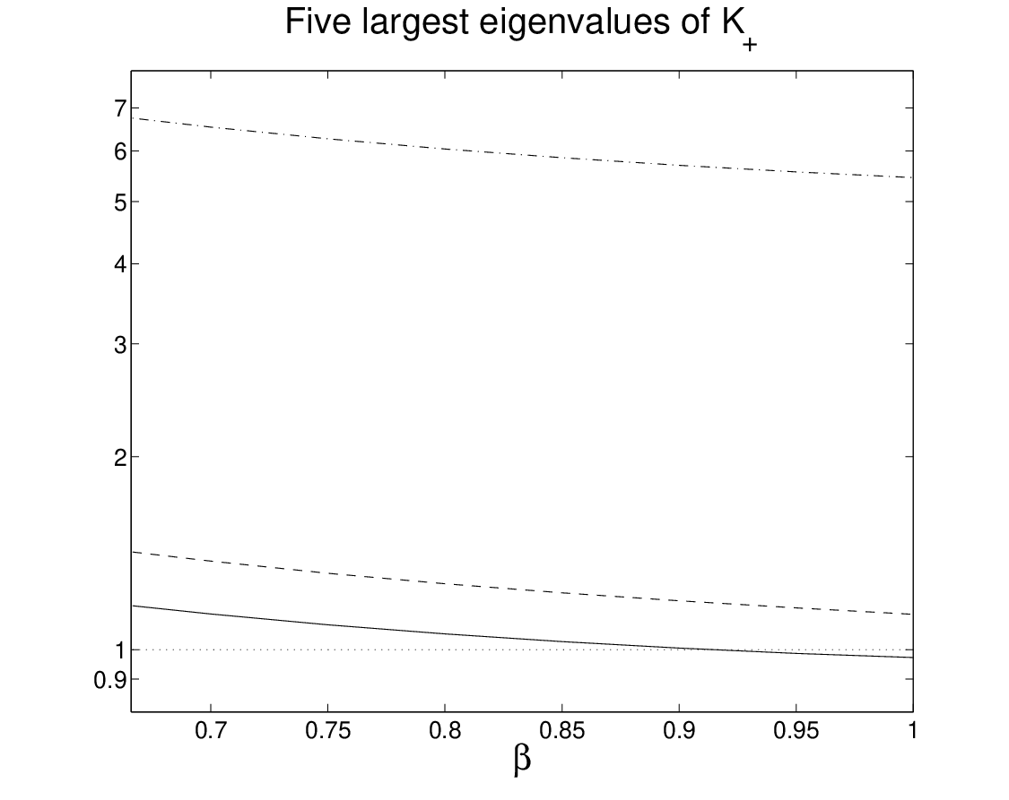
An accurate computation of the numerical value of the exceptional exponent $\beta_{*}$ requires higher values of $L$ and $N$. On a 2005 standard desktop, we have tried $L=25$ and $N=200$. We then obtain $\beta_{*}$ by interpolation of $\lambda_{5}(K_{+})$ for different closeby values of $\beta$, see table 1. The confidence on $\beta_{*}$, which we estimate to be about 8 digits, is directly related to the level of accuracy of $\lambda_{5}(K_{+})$. The latter is determined by inspection of convergence as $L$ and $N$ increase. So the bounds given in the main claim, in the introduction, are not rigorous, but merely serve as an indication of how accurate we believe our algorithm is.

$\beta$	$\lambda_{5}(K_{+})$
0.91395850	1.00000016477
0.91395875	1.00000006304
0.91395900	0.99999996130
0.91395925	0.99999985957

Table 1: Fifth eigenvalue of $K_{+}$, as a function of $\beta$ near $\beta_{*}$. Here $L=25$ and $N=200$. Each value took about one day to obtain. Cubic interpolation reveals $\beta_{*}\simeq 0.913958905\pm 1e-8$.

At this point the reader might wonder if, instead of a full three-dimensional simulation, there exists a computational strategy involving only the radial coordinate to compute both the soliton and the eigenvalues of the Birman-Schwinger operators. We believe the answer is positive, but will involve significantly different ideas from the ones presented in this paper. In particular, spectral accuracy will be more difficult to obtain. We leave the problem of determining more digits of the constant $\beta_{*}$, likely through the use of a one-dimensional method, as a challenge to the interested reader.

Finally, the Matlab code we used to generate the figures and compute an estimation of $\beta_{*}$ can be freely downloaded from

http://www.acm.caltech.edu/~demanet/NLS/.

Department of Applied and Computational Mathematics, 217-50 Caltech,
Pasadena, CA 91125, U.S.A.
email: demanet@acm.caltech.edu,

Department of Mathematics, 253-37 Caltech,
Pasadena, CA 91125, U.S.A.
email: schlag@its.caltech.edu

References

- [BerCaz] Berestycki, H., Cazenave, T. Instabilité des états stationnaires dans les équations de Schrödinger et de Klein-Gordon non linéaires. C. R. Acad. Sci. Paris Sér. I Math. 293 (1981), no. 9, 489–492.
- [BerLio] H. Berestycki, P.L. Lions, Nonlinear scalar field equations. I. Existence of a ground state. Arch. Rational Mech. Anal. 82 (1983), no. 4, 313–345.
- [BerLioPel] H. Berestycki, P.L. Lions, L.A. Peletier, An ODE approach to the existence of positive solutions for semilinear problems in . Indiana U. Math. J. 30 (1981), no. 1, 141–157.
- [BusPer1] Buslaev, V. S., Perelman, G. S. Scattering for the nonlinear Schrödinger equation: states that are close to a soliton. (Russian) Algebra i Analiz 4 (1992), no. 6, 63–102; translation in St. Petersburg Math. J. 4 (1993), no. 6, 1111–1142.
- [CazLio] Cazenave, T., Lions, P.-L. Orbital stability of standing waves for some nonlinear Schrödinger equations. Comm. Math. Phys. 85 (1982), 549–561
- [Cuc] Cuccagna, S. Stabilization of solutions to nonlinear Schrödinger equations. Comm. Pure Appl. Math. 54 (2001), no. 9, 1110–1145.
- [Eigs]
http://www.mathworks.com/access/helpdesk/help/techdoc/ref/eigs.html,
and references therein. - [ErdSch] Erdoğan, M. B., Schlag, W. Dispersive estimates for Schrödinger operators in the presence of a resonance and/or an eigenvalue at zero energy in dimension three: II, preprint 2005.
- [Flu] Flügge, S. Practical quantum mechanics. Reprinting in one volume of Vols. I, II. Springer-Verlag, New York-Heidelberg, 1974.
- [Gri] Grillakis, M. Analysis of the linearization around a critical point of an infinite dimensional Hamiltonian system. Comm. Pure Appl. Math. 41 (1988), no. 6, 747–774.
- [GriShaStr1] Grillakis, M., Shatah, J., Strauss, W. Stability theory of solitary waves in the presence of symmetry. I. J. Funct. Anal. 74 (1987), no. 1, 160–197.
- [GriShaStr2] Grillakis, M., Shatah, J., Strauss, W. Stability theory of solitary waves in the presence of symmetry. II. J. Funct. Anal. 94 (1990), 308–348.
- [HutPym] Hutson, V., Pym, J.S., Applications of Functional Analysis and Operator Theory, Academic Press, London, 1980.
- [JenKat] Jensen, A., Kato, T., Spectral properties of Schrödinger operators and time-decay of the wave functions, Duke Math. J. 46 (1979), no.3, 583–611
- [Kwo] Kwong, M. K. Uniqueness of positive solutions of in . Arch. Rat. Mech. Anal. 65 (1989), 243–266.
- [PelSte] D. Pelinovsky, Y. Stepanyants, Convergence of Petviashvili’s iteration method for numerical approximation of stationary solutions to nonlinear wave equations. SIAM J. Num. Anal. 42 (2004), no. 3, 1110–1127
- [Per2] Perelman, G. On the formation of singularities in solutions of the critical nonlinear Schrödinger equation. Ann. Henri Poincaré 2 (2001), no. 4, 605–673.
- [RodSchSof1] Rodnianski, I., Schlag, W., Soffer, A. Dispersive Analysis of Charge Transfer Models, preprint 2002, to appear in CPAM
- [RodSchSof2] Rodnianski, I., Schlag, W., Soffer, A. Asymptotic stability of -soliton states of NLS, preprint 2003, submitted to CPAM
- [Sch] Schlag, W. Stable manifolds for orbitally unstable NLS. preprint, 2004.
- [Str] Strauss, W. A. Nonlinear wave equations. CBMS Regional Conference Series in Mathematics, 73. American Mathematical Society, Providence, RI, 1989
- [SulSul] Sulem, C., Sulem, P.-L. The nonlinear Schrödinger equation. Self-focusing and wave collapse. Applied Mathematical Sciences, 139. Springer-Verlag, New York, 1999.
- [Wei1] Weinstein, Michael I. Modulational stability of ground states of nonlinear Schrödinger equations. SIAM J. Math. Anal. 16 (1985), no. 3, 472–491.
- [Wei2] Weinstein, Michael I. Lyapunov stability of ground states of nonlinear dispersive evolution equations. Comm. Pure Appl. Math. 39 (1986), no. 1, 51–67.