Skein relations for Milnor’s $\mu$-invariants

Abstract

The theory of link-homotopy, introduced by Milnor, is an important part of the knot theory, with Milnor’s $\bar{\mu}$-invariants being the basic set of link-homotopy invariants. Skein relations for knot and link invariants played a crucial role in the recent developments of knot theory. However, while skein relations for Alexander and Jones invariants are known for quite a while, a similar treatment of Milnor’s $\bar{\mu}$-invariants was missing. We fill this gap by deducing simple skein relations for link-homotopy $\mu$-invariants of string links.

57M25 57M27

  ATG Volume 5 (2005) 1471–1479Published: 30 October 2005

Abstract

AMS Classification;

Keywords

1 Introduction

1.1 Some history

Skein relations for various invariants played a significant role in knot theory and related areas in the last decade. Probably the first widely-used skein relation, discovered by Conway, was the skein relation for the Conway-Alexander polynomial. Apart from multiple technical consequences, it led to the discovery of similar skein relations for other knot invariants, notably for the Jones and HOMFLY polynomials. In the theory of 3-manifolds, the skein relation for the Casson invariant of homology spheres was also fruitfully used in different contexts.

An important part of the knot theory is the theory of link-homotopy, initiated by Milnor. Link-homotopy is a useful notion to isolate the linking fenomena from the self-knotting ones and to study it separately. A celebrated example of link-homotopy invariants is given by Milnor’s $\bar{\mu}_{{i_{1}\dots i_{r}},j}$ invariants [4, 5] with non-repeating indices $1\leq i_{1},\dots i_{r},j\leq n$. Roughly speaking, these describe the dependence of $j$-th parallel on the meridians of $i_{1}$-th, …, $i_{r}$-th components. The simplest invariant $\bar{\mu}_{i,j}$ is just the linking number of the corresponding components. The next one, $\bar{\mu}_{i_{1}i_{2},j}$, detects the Borromean-type linking of the corresponding 3 components and, together with the linking numbers, classify 3-component links up to link-homotopy.

Unfortunately, a complicated self-recurrent indeterminacy in the definition of $\bar{\mu}$-invariants (reflected in the use of notation $\bar{\mu}$, rather than $\mu$) for a long time slowed down their study. The introduction of string links [2] considerably improved the situation, since a version of $\bar{\mu}$-invariants modified for string links is free of this indeterminacy; thus (and to stress a special role of the $j$-th component) we will further use the notation $\mu_{i_{1}\dots i_{r}}(L,L_{j})$ for these invariants. Milnor’s invariants classify string links up to link-homotopy [2]. Surprisingly, up to now $\mu$-invariants remained aside from the well-developed scheme of skein relations.

1.2 Brief statement of results

We deduce new skein relations for $\mu$-invariants. Usually in the knot theory skein relations involve links, obtained by different splittings of a diagram in a crossing. In the context of string links this leads to an appearance of tangles which are not pure any more, but contain a new “loose” component. Fortunately, it is easy to extend the definition of $\mu$-invariants to such tangles. We next note that $\mu_{i_{1}\dots i_{r}}(L,l)=0$ for any string link $L$ whose loose component $l$ passes everywhere in front of the other strings. Thus it suffices to study the jump of $\mu_{i_{1}\dots i_{r}}$ under a crossing change of $l$ with any other, say, $i_{k}$-th, component. It turns out, that this jump can be expressed via the invariants $\mu_{i_{1}\dots i_{k-1}}(L-L_{i_{k}},l_{0})$ and $\mu_{i_{k+1}\dots i_{r}}(L-L_{i_{k}},l_{\infty})$ of string links with new loose components $l_{0}$ and $l_{\infty}$ obtained by splitting the crossing in two possible ways, see Section 3.1.

This research was partially supported by C. Wellner Research fund and 6th EC Programme “Structuring the European Research Area”, contract Nr. RITA-CT-2004-505493

2 Preliminaries

2.1 String links and link-homotopy

Let $D^{2}$ be a disc in the $xy$-plane which intersects the $x$-axis. An $n$-component string link (see [3], [2]) $L$ is an ordered collection of $n$ disjoint arcs properly embedded in $D^{2}\times[0,1]$ in such a way, that the $i$-th arc ends in the points $p_{i}\times\{0,1\}$, where $p_{i}=(x_{i},0)$ are some prescribed points on the $x$-axis, enumerated in the natural order $x_{1}<x_{2}<\dots<x_{n}$. We assume that all arcs of $L$ are oriented downwards. By the closure $\overline{L}$ of a string link $L$ we mean the braid closure of $L$. It is an $n$-component link obtained from $L$ by an addition of $n$ disjoint arcs in the plane $\{y=0\}$, each of which meets $D^{2}\times[0,1]$ only at the endpoints $p_{i}\times\{0,1\}$ of $L$, as illustrated in Figure 1. The linking number $\operatorname{lk}$ of two components of $L$ is their linking number in $\overline{L}$.

 

Figure 1: String link and its closure

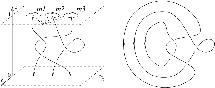
Two string links are link-homotopic, if one can be transformed into the other by homotopy, which fails to be isotopy only in a finite number of instants, when a (generic) self-intersection point appears on one of the arcs.

2.2 String links with a loose component

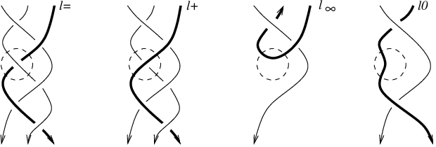
Further we will consider a more general class of tangles. A $n$-component string link $L$ with an additional loose component $l$ is a pair $(L,l)$ which consists of an $n$-string link $L$ together with an additional oriented arc $l$ properly embedded in $D^{2}\times[0,1]$ in such a way, that $l\cap L=\emptyset$ and $l$ starts on $D^{2}\times\{1\}$ and ends on $D^{2}\times\{0,1\}$. See Figure 2, where loose components are depicted in bold. By the closure $\overline{(L,l)}$ of a string link $L$ with a loose component $l$ we mean the closure of $L$, together with a closure of $l$ by a standard arc in $\mathbb{R}^{3}-D^{2}\times(0,1)$, which meets $l$ only at its endpoints and passes “in front” of $L$ i.e. lies in the half-space $y\geq 0$, as illustrated in Figure 2.

 

Figure 2: 2-component string links with a loose component and their closures

In particular, for any $n$-string link $L=\cup_{i=1}^{n}L_{i}$ and $1\geq j\geq n$ one may consider $(L-L_{j},L_{j})$ as an $(n-1)$-string link with an additional loose component $L_{j}$. In this case it does not matter whether to close $L_{j}$ in front of $L$ or in the plane $\{y=0\}$ and closures $\overline{L}$ and $\overline{(L-L_{j},L_{j})}$ give isotopic links.

2.3 Magnus expansion

Milnor’s link-homotopy $\mu$-invariants [4] can be defined in several ways. We choose a construction most suitable for our purposes and refer the reader to Milnor’s work [4, 5] and its adaptations to string links (e.g. [3], [2]) for the general case.

Let $L=\cup_{i=1}^{n}L_{i}$ be an $n$-component string link. Consider the link group $\pi=\pi_{1}(D^{2}\times[0,1]-L)$ (with the base point on the upper boundary disc $D^{2}\times\{1\}$). Denote by $m_{i}\in\pi$, $i=1,\dots,n$ the canonical meridians represented by the standard non-intersecting curves in $D^{2}\times\{1\}$ with $\operatorname{lk}(m_{i},L_{i})=+1$, as shown in Figure 1. If $L$ would be a braid, these meridians would freely generate $\pi$, with any other meridian of $L_{i}$ in $\pi$ being a conjugate of $m_{i}$. For the string links, similar results hold for the reduced link group $\tilde{\pi}$.

For any group $G$ with a finite set of generators $x_{1},\dots x_{n}$, the reduced group $\tilde{G}$ is the factor group of $G$ by relations $[x^{\prime}_{i},x^{\prime\prime}_{i}]=1$, $i=1,\dots,n$ for any two elements $x^{\prime}_{i}$ and $x^{\prime\prime}_{i}$ in the conjugacy class of $x_{i}$.

Proceeding similarly to the usual construction of Wirtinger’s presentation, one can show (see [2]) that $\tilde{\pi}$ is generated by $m_{i}$. Let $F$ be the free group on $n$ generators $x_{1},\dots x_{n}$. The map $F\to\pi$ defined by $x_{i}\mapsto m_{i}$ induces the isomorphism $\widetilde{F}\cong\tilde{\pi}$ of the reduced groups [2]. We will use the same notation for the elements of $\pi$ and their images in $\tilde{\pi}\cong\widetilde{F}$.

Now, let $\mathbb{Z}[[X_{1},\dots,X_{n}]]$ be the ring of power series in $n$ non-commuting variables $X_{i}$ and denote by $\widetilde{Z}$ its factor by all the monomials, where at least one of the generators appears more than once. The Magnus expansion is a ring homomorphism of the group ring $\mathbb{Z}F$ into $\mathbb{Z}[[X_{1},\dots,X_{n}]]$, defined by $x_{i}\mapsto 1+X_{i}$. It induces the homomorphisms $\theta:\mathbb{Z}\widetilde{F}\to\widetilde{Z}$ and $\theta_{L}:\mathbb{Z}\tilde{\pi}\to\widetilde{Z}$ of the corresponding reduced group rings.

2.4 Milnor’s $\mu$-invariants

Let $l$ an immersed arc in $D^{2}\times[0,1]-L$ with $\partial l\in R^{1}\times\{0\}\times\{0,1\}$. Its closure by an arc on the boundary of the cylinder $D^{2}\times[0,1]$ in front of $L$ (i.e. in the half-space $y\geq 0$) gives a well-defined loop $\bar{l}$ in $\tilde{\pi}$. Thus one may define the Milnor’s invariants $\mu_{{i_{1}\dots i_{r}}}(L,l)$ of a string link with a loose component $(L,l)$ as coefficients of the Magnus expansion $\theta_{L}(\bar{l})$ of $\bar{l}$:

$$\theta_{L}(l)=\sum\mu_{{i_{1}\dots i_{r}}}(L,l)X_{i_{1}}X_{i_{2}}\dots X_{i_{r}}\ .$$

Note that if $l$ goes in front of $L$, i.e. overpasses all other components on the $xz$-plane diagram of $L\cup l$, then all invariants $\mu_{{i_{1}\dots i_{r}}}(L,l)$ vanish. Indeed, we choose to close $l$ in the front half-space $\{y\geq 0\}\cap\partial(D^{2}\times[0,1])$, so the loop $\bar{l}$ is trivial in $\pi$ (and hence trivial in $\tilde{\pi}$).

For string links, Milnor’s invariants $\mu_{{i_{1}\dots i_{r}}}(L-L_{j},L_{j})$ are usually denoted by $\mu_{{i_{1}\dots i_{r}},j}(L)$ (see e.g. [3], [2]). Modulo lower degree invariants $\mu_{{i_{1}\dots i_{r}}}(L-L_{j},L_{j})\equiv\bar{\mu}_{{i_{1}\dots i_{r}},j}(\overline{L})$, where $\bar{\mu}_{{i_{1}\dots i_{r}},j}(\overline{L})$ are the original Milnor’s link invariants [4, 5].

2.5 Fox’s free calculus

Instead of the Magnus expansion, $\mu$-invariants may be defined via Fox free calculus.

Fox’s free derivatives $\delta_{i}:\mathbb{Z}F\to\mathbb{Z}F$, $i=1,\dots,n$, are defined by putting $\delta_{i}1=0$, $\delta_{i}x_{i}=1$, $\delta_{i}x_{j}=0$, $j\neq i$ and extending the function $\delta_{i}$ to $\mathbb{Z}F$ by linearity and the rule $\delta_{i}(uv)=\delta_{i}u+u\cdot\delta_{i}v$, $u,v\in ZF$. In particular, it is easy to see that $\delta_{i}(x_{i}^{-1})=-x_{i}$. For $u\in\mathbb{Z}F$, denote by $\delta_{i_{1}}\dots\delta_{i_{r}}u(1)\in\mathbb{Z}$ the value of $\delta_{i_{1}}\dots\delta_{i_{r}}u$ in $x_{1}=\dots=x_{n}=1$.

Free derivatives in $\mathbb{Z}F$ induce similar Fox derivatives $\delta_{i}:\mathbb{Z}\widetilde{F}\to\mathbb{Z}\widetilde{F}$ and $\delta_{i}:\mathbb{Z}\tilde{\pi}\to\mathbb{Z}\tilde{\pi}$ in the reduced group rings. From the definition of $\mu$-invariants we conclude that $\mu_{{i_{1}\dots i_{r}}}(L,l)=\delta_{i_{1}}\dots\delta_{i_{r}}l(1)$.

3 Skein relations for $\mu$-invariants

3.1 Main Theorem

Consider two $n$-string links $(L,l_{+})$ and $(L,l_{-})$ with loose components such that their diagrams coincide everywhere, except for a crossing $d$, where $l_{+}$ has the positive crossing and $l_{-}$ the negative crossing with $i_{k}$-th component $L_{i_{k}}$ of $L$, see Figure 3.

 

Figure 3: Splitting the link in a crossing

We define two new $(n-1)$-string links with loose components by splitting the diagram in $d$ in two possible ways. Let $l_{\infty}$ be the component of the splitting going along $l$, respecting the orientation, and then switching to $L_{i_{k}}$ against the orientation. Let also $l_{0}$ be the component going first along $L_{i_{k}}$ and then along $l$, respecting the orientation. Each of $(L-L_{i_{k}},l_{0})$ and $(L-L_{i_{k}},l_{\infty})$ is a $(n-1)$-string link with a loose component, see Figure 3.

Theorem 3.1.

Let $L$, $l_{\pm}$, $l_{0}$ and $l_{\infty}$ be as above. Then

$$\mu_{i_{1}\dots i_{k}\dots i_{r}}(L,l_{+})-\mu_{i_{1}\dots i_{k}\dots i_{r}}(L,l_{-})=\mu_{i_{1}\dots i_{k-1}}(L-L_{i_{k}},l_{\infty})\cdot\mu_{i_{k+1}\dots i_{r}}(L-L_{i_{k}},l_{0}).$$

Here it is understood that in particular cases $k=1$ or $k=r$ we have

$$\mu_{i_{k}}(L,l_{+})-\mu_{i_{k}}(L,l_{-})=1;$$

$$\mu_{i_{1}\dots i_{k}}(L,l_{+})-\mu_{i_{1}\dots i_{k}}(L,l_{-})=\mu_{i_{1}\dots i_{k-1}}(L-L_{i_{k}},l_{\infty});$$

$$\mu_{i_{k}\dots i_{r}}(L,l_{+})-\mu_{i_{k}\dots i_{r}}(L,l_{-})=\mu_{i_{k+1}\dots i_{r}}(L-L_{i_{k}},l_{0}).$$

Example 3.2.

Consider the string link $(L,l)$ depicted in Figure 4 and let us compute $\mu_{12}(L,l)$. Notice that if we switch the crossing $d$ to the positive one, we get a link $(L,l_{+})$ with $L_{1}$ unlinked from $L_{2}$ and $l_{+}$, so $\mu_{12}(L,l_{+})=0$. Thus $\mu_{12}(L,l)=\mu_{12}(L,l)-\mu_{12}(L,l_{+})=-\mu_{1}(L_{1},l_{\infty})=-1$, in agreement with the fact that the closure of $(L,l)$ is the (negative) Borromean link.

 

Figure 4: A computation of $\mu_{12,3}$ for Borromean rings

3.2 The proof of Theorem 3.1

We will need the following simple key fact about Fox free calculus, which we leave to the reader as an exercise:

Lemma 3.3.

Let $1\leq k\leq r<j\leq n$ and $\varepsilon=\pm 1$. Then for any $u,v\in F$

$$\delta_{1}\dots\delta_{r}(ux_{k}^{\varepsilon}v)(1)=\varepsilon\cdot\delta_{1}\dots\delta_{k-1}u(1)\cdot\delta_{k+1}\dots\delta_{r}v(1)+\delta_{1}\dots\delta_{r}(uv)(1).$$ (1)

Also, to simplify the notations in the statement of Theorem 3.1, let us reorder the components so that $i_{m}\to m$, $m=1,\dots r$ (and $j\neq 1,\dots,r$).

Proof of Theorem 3.1.

The component $l_{+}$ passes either over, or under $L_{k}$ in the crossing $d$. Let us consider these cases separately. Assume first that $l_{+}$ passes under $L_{k}$ in $d$. Then $l_{+}=vu^{-1}x_{k}uw$, where $v$ and $w$ are the parts of $l_{+}$ before and after $d$, and $u$ is the part of $l_{k}$ before $d$, see Figure 5.

 

Figure 5: Computing $l_{+}$ and $l_{-}$

Thus, by the definition of $\mu_{1\dots k\dots r}(L,l)$ and (1) we have

$$\mu_{1\dots r}(L,l_{+})=\delta_{1}\dots\delta_{r}(vu^{-1}x_{k}uw)(1)=\\ \delta_{1}\dots\delta_{k-1}(vu^{-1})(1)\cdot\delta_{k+1}\dots\delta_{r}(uw)(1)+\delta_{1}\dots\delta_{r}(vw)(1).$$

Now, $l_{-}$ passes over $L_{k}$, so $l_{-}=vw$, where again $v$ and $w$ are the parts of $l_{-}$ before and after $d$, see Figure 5. Thus

$$\mu_{1\dots k\dots r}(L,l_{-})=\delta_{1}\dots\delta_{k}\dots\delta_{r}(vw)(1).$$

Therefore

$$\mu_{1\dots k\dots r}(L,l_{+})-\mu_{1\dots k\dots r}(L,l_{-})=\delta_{1}\dots\delta_{k-1}(vu^{-1})(1)\cdot\delta_{k+1}\dots\delta_{r}(uw)(1).$$

But $vu^{-1}$ and $uw$ are exactly $l_{\infty}$ and $l_{0}$, see Figure 6.

 

Figure 6: Computing $l_{\infty}$ and $l_{0}$

It remains to use again the definition of $\mu$-invariants to obtain

$$\mu_{1\dots k\dots r}(L,l_{+})-\mu_{1\dots k\dots r}(L,l_{-})=\mu_{1\dots k-1}(L,l_{\infty})\cdot\mu_{k+1\dots r}(L,l_{0}).$$

In the case when $l_{+}$ passes over $L_{k}$ at the crossing $d$, the proof is completely similar. This time $l_{-}=vu^{-1}x_{k}^{-1}uw$ and $l_{+}=vw$, thus basically we just exchange $l_{+}$ and $l_{-}$ in the previous proof. Also, the degree of $x_{k}$ switches from $+1$ to $-1$, which leads to the negative sign in the application of (1) and cancels out with the sign appearing from the exchange of $L_{+}$ and $L_{-}$. ∎

Received:9 August 2005

References

- [1] M Goussarov, M Polyak, O Viro, Finite-type invariants of classical and virtual knots, Topology 39 (2000) 1045–1068 \MR1763963
- [2] N Habegger, X-S Lin, The classification of links up to link-homotopy, J. Amer. Math. Soc. 3 (1990) 389–419 \MR1026062
- [3] J P Levine, The -invariants of based links, from: “Differential topology (Siegen, 1987)”, Lecture Notes in Math. 1350, Springer, Berlin (1988) 87–103 \MR979334
- [4] J Milnor, Link groups, Ann. of Math. (2) 59 (1954) 177–195 \MR0071020
- [5] J Milnor, Isotopy of links, from: “Algebraic geometry and topology, A symposium in honor of S Lefshetz”, Princeton Univ. Press (1957) 280–306 \MR0092150
- [6] M Polyak, On Milnor’s triple linking number, C. R. Acad. Sci. Paris Sér. I Math. 325 (1997) 77–82 \MR1461401
- [7] M Polyak, O Viro, Gauss diagram formulas for Vassiliev invariants, Internat. Math. Res. Notices (1994) 445–452 \MR1316972
Received:\qua9 August 2005