The planar algebra of a semisimple and cosemisimple Hopf algebra

Abstract.

To a semisimple and cosemisimple Hopf algebra over an algebraically closed field, we associate a planar algebra defined by generators and relations and show that it is a connected, irreducible, spherical, non-degenerate planar algebra with non-zero modulus and of depth two. This association is shown to yield a bijection between (the isomorphism classes, on both sides, of) such objects.

Throughout this paper, the symbol ${\bf k}$ will always denote an algebraically closed field and $H=(H,\mu,\eta,\Delta,\epsilon,S)$ will always denote a semisimple and cosemisimple (necessarily finite-dimensional) Hopf algebra over ${\bf k}$. We associate to $H$, a planar algebra over the field ${\bf k}$ which is an analogue of the construction in [KdyLndSnd] of the ‘subfactor planar algebra’ associated to a (finite-dimensional) Kac algebra.

We then study various properties of this planar algebra including computation of its partition function and duality with the planar algebra of $H^{*}$. Conversely, we show that every connected, irreducible, spherical, non-degenerate planar algebra with non-zero modulus and of depth two arises in this manner, thus obtaining a generalisation of the Ocneanu-Szymanski theorem (cf. [Szy]).

1. Semisimple and cosemisimple Hopf algebras

We begin by recalling well-known facts about such an $H$, the proofs of which may be found in [TngGlk] and in [LrsRdf]. The semisimplicity and cosemisimplicity assumptions imply that both $H$ and $H^{*}$ are multi-matrix algebras and the dimensions, say $n$, of $H$, as well as those of its irreducible representations, are ‘non-zero in ${\bf k}$’. It follows that the traces in the regular representations of $H$ and $H^{*}$, which we shall denote by $\phi$ and $h$ respectively, are non-degenerate traces. Further, these are two-sided integrals for $H^{*}$ and $H$ respectively : i.e., they satisfy $\phi\psi=\psi(1)\phi=\psi\phi$ and $hx=\epsilon(x)h=xh$, for all $\psi\in H^{*}$ and $x\in H$. Also, $\epsilon(h)=\phi(h)=\phi(1)=n\in{\bf k}$. Finally, the antipodes of $H$ and $H^{*}$ are involutive.

We shall use the standard notations $\mu_{k}$ and $\Delta_{k}$ for the $k$-fold iterated product and coproduct respectively. In particular, $\mu_{0}=\eta$, $\mu_{1}=id_{H}$, $\mu_{2}=\mu$ and $\Delta_{0}=\epsilon$, $\Delta_{1}=id_{H}$ and $\Delta_{2}=\Delta$. We will find it convenient to use our version of the so-called Sweedler notation for comultiplication - according to which we write, for example, $\Delta_{n}(x)=x_{1}\otimes\cdots\otimes x_{n}$ rather than the more familiar $\Delta_{n}(x)=\sum_{(x)}x_{(1)}\otimes\cdots\otimes x_{(n)}$ in the interest of notational convenience.

2. Planar algebras

We will also need the formalism of Jones’ planar algebras. Although Jones primarily used planar algebras which are $C^{*}$-planar algebras, and à fortiori defined over $\mathbb{C}$, we need their analogues over more general fields here, so we give a ‘crash course’ accordingly; but by and large, we assume familiarity with planar tangles, planar networks and planar algebras. The basic reference is [Jns]. A somewhat more leisurely treatment of the basic notions may also be found in [KdySnd]. (We will follow the latter where, for instance, the $*$’s are attached to ‘distinguished points’ on boxes rather than to regions and for notation such as $1_{k}$ for the identity element of $P_{k}$ for a planar algebra $P$.)

We shall continue to use the term planar tangle, as well its colour, in exactly the same sense as used in [KdySnd]. By a planar algebra $P$ (over ${\bf k}$), we shall mean a collection $\{P_{k}:k\in Col\}$ of ${\bf k}$-vector spaces, indexed by the set $Col=\{0_{+},0_{-},1,2,\cdots\}$ of ‘colours’, which comes equipped with the following structure: to each $k_{0}$-tangle $T$ (with internal boxes $B_{1},\cdots,B_{g}$ of colours $k_{1},\cdots,k_{g}$) is associated a ${\bf k}$-linear mapping $Z^{P}_{T}:\otimes_{i=1}^{g}P_{k_{i}}\rightarrow P_{k_{0}}$ which satisfies several natural conditions (listed as equations (2.2), (2.3), (2.4) and (2.6) in [KdySnd]).

Given a ‘label set’ $L=\coprod_{k\in Col}L_{k}$, an L-labelled tangle is a tangle $T$ equipped with a labelling of every internal box of colour $k$ by an element from $L_{k}$. The universal planar algebra on $L$, denoted by $P(L)=\{P(L)_{k}:k\in~Col\}$ is defined by requiring that $P(L)_{k}$ is the ${\bf k}$-vector space with basis consisting of the set of all $L$-labelled $k$-tangles, with the action of a planar tangle on a tensor product of basis vectors given by $L$-labelled tangles being the obvious $L$-labelled tangle obtained by substitution.

Recall that a planar ideal of a planar algebra $P$ is a set $I=\{I_{k}:k\in~Col\}$ with the property that (i) each $I_{k}$ is a subspace of $P_{k}$, and (ii) for any $k_{0}$-tangle $T$ as before, $Z_{T}(\otimes_{i=1}^{g}x_{i})\in I_{k_{0}}$ whenever $x_{i}\in I_{k_{i}}$ for at least one $i$. Given a planar ideal $I$ in a planar algebra $P$, there is a natural planar algebra structure on the ‘quotient’ $P/I=\{P_{k}/I_{k}:k\in~Col\}$.

Given any subset $R=\{R_{k}:k\in~Col\}$ of $P$ (meaning $R_{k}\subset P_{k}$), there is a smallest planar ideal $I(R)=\{I(R)_{k}:k\in~Col\}$ such that $R_{k}\subset I(R)_{k}$ for all $k\in Col$; and finally, given a label set $L$ as above, and any subset $R$ of the universal planar algebra $P(L)$, the quotient $P(L)/I(R)$ is said to be the planar algebra $P(L,R)$ presented with generators $L$ and relations $R$.

3. Definition of $P(H,\delta)$

Motivated by the results of [KdyLndSnd] - where the case of the so-called finite-dimensional Kac-algebras (over $\mathbb{C}$) is treated - we wish to define the planar algebra associated to a semisimple and cosemisimple Hopf algebra via generators and relations.

However, our definition will depend on a choice we have to make of a square root in ${\bf k}$ of $n$. To be precise, we shall let $\delta$ be a solution to $\delta^{2}=n$ in ${\bf k}$, and then define $P(H,\delta)$ to be the planar algebra $P(L,R)$, with

$$L_{k}=\left\{\begin{array}[]{ll}H&{\mbox{if}}~k=2\\ \emptyset&{\mbox{otherwise}}\end{array}\right.$$

and  $R$ being given by the set of relations in Figures 1 - 4 (where (i) we write the relations as identities - so the statement $a=b$ is interpreted as $a-b\in R$; (ii) $\zeta\in{\bf k}$ and $a,b\in H$; and (iii) the external boxes of all tangles appearing in the relations are left undrawn and it is assumed that all external $*$’s are at the top left corners).

Figure 1. The L(inearity) and M(odulus) relations

Figure 2. The U(nit) and I(ntegral) relations

Figure 3. The C(ounit) and T(race) relations

Figure 4. The E(xchange) and A(ntipode) relations

We note that relation (M) actually represents two relations, one in $P_{0_{+}}$ and the other in $P_{0_{-}}$ and that the $\delta$ in relation (M) means $\delta 1_{0_{+}}$ in one of the relations and $\delta 1_{0_{-}}$ in the other.

In the rest of this paper, we shall simply write $P$ for the planar algebra $P(H,\delta)$.

4. Properties of $P$

We wish to study the properties of $P$. Recall that a planar algebra $P$ is said to be connected if $dim~P_{0_{\pm}}=1$ and irreducible if $dim~P_{1}=1$. A connected planar algebra is said to have modulus $\delta$ if the relation (M) holds in $P$.

We will need some facts concerning ‘exchange relation planar algebras’ as defined in [Lnd]. Although only planar algebras over $\mathbb{C}$ are considered there, the proofs of some results we need from there are seen to carry over verbatim for general ${\bf k}$. We isolate one such fact from [Lnd] as a lemma below, which we will need to use repeatedly in the sequel.

Lemma 1.

In any ‘exchange relation planar algebra’ $P$, and for any $k\in Col$, the space $P_{k}$ is linearly spanned by the images of labelled $k$-tangles with at most $k-1$ internal boxes (all of colour $2$ and where we take $k-1=0$ if $k=0_{\pm}$) that have no ‘internal faces’.

Rather than repeating the definition of an ‘exchange relation planar algebra’ here, it will suffice for the reader to know that if $L=L_{2}=H$ and $R_{0}$ is any set of relations which contains $R\setminus\{U,I\}$, then $P(L,R_{0})$ is an exchange relation planar algebra.

Proposition 2.

The planar algebra $P$ is a connected planar algebra.

Proof.

We deduce from Lemma 1 that $P_{0_{\pm}}$ is linearly spanned by its identity element $1_{0_{\pm}}$ (since $1^{0_{\pm}}$ is the only $0_{\pm}$-tangle ‘without internal faces’). Thus, $dim~P_{0_{\pm}}\leq 1$.

To prove the reverse inequality, we construct a functional $\lambda_{\pm}:P(L)_{0_{\pm}}\rightarrow{\bf k}$ which is non-trivial and show that it descends to the quotient $P_{0_{\pm}}$ of $P(L)_{0_{\pm}}$ by $I(R)_{0_{\pm}}$. The motivation for the definition of $\lambda_{\pm}$ comes from the description of the partition function of $P(H)$ given in [Lnd] for $H={\mathbb{C}}[G]$ and generalised in [KdyLndSnd] for a Kac algebra $H$.

The functional $\lambda_{\pm}$ is defined by specifying it on a basis of $P(L)_{0_{\pm}}$, a typical element of which is an $L$-labelled $0_{\pm}$-tangle. Since $L_{k}=\emptyset$ for $k\neq 2$, each internal box of such a tangle is necessarily a $2$-box. It will be easiest to illustrate the prescription in a particular example. Consider, for instance, the $0_{+}$-tangle $T$ shown on the left in Figure 5. (We will identify $0_{+}$-tangles (resp. $0_{-}$-tangles) with planar networks with unbounded region of colour white (resp. black) by removing the external box.)

Figure 5. The procedure for calculating $\tau_{+}$

Removing each labelled $2$-box - with label $l$ (say) - and inserting a symbol $l_{1}$ close to the strand through the $*$ of the box and a symbol $Sl_{2}=S(l_{2})$ close to the other strand yields the picture on the right of Figure 5.

Now arbitrarily pick a base point on each component (loop) of the resulting figure, read the labels on that component in the order opposite to that prescribed by the orientation of the loop, evaluate $\delta^{-1}\phi$ on each resulting product (the empty ‘product’ being $1$ if the loop has no labels) and multiply the answers. Thus, in our example, we would obtain

$$\delta^{-1}\phi(a_{1}(Sd_{2})c_{1})~\delta^{-1}\phi((Sc_{2})(Sb_{2})(Sa_{2}))~\delta^{-1}\phi(b_{1}d_{1})~,$$

and this element of ${\bf k}$ is what we will define as $\lambda_{+}(T)$. Note that the answer is independent of the choices of base-points since $\phi$ is a trace. The same procedure is used to define $\lambda_{-}$ on $P(L)_{0_{-}}$. Observe that two $0$-tangles (possibly one $0_{+}$ and the other $0_{-}$) whose associated planar networks are isotopic on the sphere $S^{2}$ yield the same element of ${\bf k}$ under the appropriate $\lambda$’s.

We now assert that $\lambda_{\pm}$ vanishes on $I(R)_{0_{\pm}}$. To see this, it suffices to see that if two (linear combinations of) $L$-labelled $0_{\pm}$-tangles differ by an application of any of the relations in $R$, then $\lambda_{\pm}$ assigns the same value to both. For all but relation (I), this follows - and we leave it to the reader to verify - from various properties of and identities in $H$ which we will list out.

• Relation (L) : Linearity of $(id\otimes S)\circ\Delta$.

• Relation (M) : $\phi(1)=\delta^{2}$.

• Relation (U) : $\Delta(1)=1\otimes 1$.

• Relation (C) : $a_{1}Sa_{2}=\epsilon(a).1_{H}$.

• Relation (T) : $a_{1}\phi(Sa_{2})=\phi(a).1_{H}$.

• Relation (E) : $a_{1}\otimes b_{1}\otimes Sb_{2}Sa_{2}=a_{1}\otimes Sa_{2}(a_{3}b_{1})\otimes S(a_{4}b_{2})$.

• Relation (A) : $(Sa)_{1}\otimes S(Sa)_{2}=Sa_{2}\otimes a_{1}$.

The verification that $\lambda_{\pm}$ assigns the same value to two $L$-labelled $0_{\pm}$-tangles that differ at a single $2$-box by an application of the relation (I) needs a little work. First, use isotopy on $S^{2}$ to move the point at infinity to a point in the white region near the $*$ of the special $2$-boxes of both (at which they differ). It should then be clear that the two tangles necessarily have the forms in Figure 6 where $X$ is some $L$-labelled $2$-tangle.

Figure 6. Two tangles that differ by the relation (I)

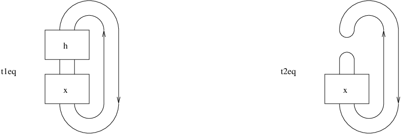
What we need to verify is that $\lambda_{+}(T_{1})=\delta\lambda_{+}(T_{2})$, where the $\delta$ factor comes from the relation (I).

Let $R_{0}=R\setminus\{I\}$. An application of Lemma 1 to $P(L,R_{0})_{2}$ shows now that the image of $X$ in $P_{2}$ may be expressed, using the relations other than (I), as a linear combination of (images of) labelled $2$-boxes and the tangle ${\mathcal{E}}^{2}$ shown in Figure 7. (Tangles ${\mathcal{E}}^{3}$ and ${\mathcal{E}}^{4}$ are shown, in order to indicate a whole sequence of tangles ${\mathcal{E}}^{k}$.)

Figure 7. The tangles ${\mathcal{E}}^{2},{\mathcal{E}}^{3}$ and ${\mathcal{E}}^{4}$

Since we have already verified that $\lambda_{\pm}$ is invariant under application of any of the relations other than (I), we reduce immediately to the case that $X$ itself is either a labelled $2$-box or the tangle ${\mathcal{E}}^{2}$. We treat these cases one by one.

If $X$ is a $2$-box labelled by $a\in H$, then the procedure for calculating $\lambda_{+}$ yields $\lambda_{+}(T_{1})=\delta^{-1}\phi(h_{1}a_{1})\delta^{-1}\phi(Sh_{2}Sa_{2})=\delta^{2}\epsilon(a)$ while $\lambda_{+}(T_{2})=\delta^{-1}\phi(Sa_{2}a_{1})=\delta\epsilon(a)$. On the other hand, if $X={\mathcal{E}}^{2}$, then $\lambda_{+}(T_{1})$ may be computed to be $\delta^{-1}\phi(h_{1}Sh_{2})=\delta^{3}$ while $\lambda_{+}(T_{2})$ is computed to be $\delta^{-2}\phi(1)\phi(1)=\delta^{2}$. In either case, we see that $\lambda_{+}(T_{1})=\delta\lambda_{+}(T_{2})$. This completes verification of invariance under the relation (I).

Thus $\lambda_{\pm}$ descend to give maps from $P_{0_{\pm}}\rightarrow{\bf k}$ that are clearly (since $\lambda_{\pm}(1_{0_{\pm}})=1$) surjective, thereby establishing that $dim~P_{0_{\pm}}\geq 1$ and concluding the proof. $\Box$

Before stating our next result, note that since for any planar algebra $P$, each $P_{k}$ is a ${\bf k}$-algebra with identity $1_{k}$, it follows that if $P$ is connected, there are canonical identifications $P_{0_{\pm}}={\bf k}$ (under which $1_{0_{\pm}}$ is identified with $1$). Consequently, if $N$ is any planar network then its partition function $Z^{P}_{N}$ takes values in ${\bf k}$.

Corollary 3.

For any labelled planar network $N$ in $P(L)_{0_{\pm}}$, its value (as given by the partition function of $P$) is $\lambda_{\pm}(N)$.

Proof.

By Lemma 1, any $L$-labelled $0_{\pm}$-tangle may be written, using all the relations in $R$, as a multiple of $1^{0_{\pm}}$ - the only $0_{\pm}$-tangle without internal faces. Since $\lambda_{\pm}$ is invariant under the relation $R$, it suffices to verify that for the tangle $1^{0_{\pm}}$, both the partition function and $\lambda_{\pm}$ assign the same value. This is true since both give the value $1$ to $1^{0_{\pm}}$, establishing the corollary. $\Box$

Since we have now verified that $P_{0_{\pm}}$ is $1$-dimensional, and in particular that its identity $1_{0_{\pm}}$ is non-zero, the following equation for $x\in P_{k}$ where $k\geq 1$,

$$Z^{~\,P}_{Tr(k)}(x)=\delta^{k}\tau_{k}(x)1_{0_{+}},$$

uniquely defines a tracial linear functional $\tau_{k}$ on $P_{k}$ which will be referred to as the normalised picture trace. Here $Tr(k)$ denotes the $0_{+}$-tangle with a single internal $k$-box that is shown in Figure 8.

Figure 8. The trace tangle

Note that $\tau_{k}(1_{k})=1$.

Let $\pi$ denote the natural map from $H$ to $P_{2}$ which takes $a\in H$ to the image of the $2$-box labelled by $a$. We then have the following lemma by which we will henceforth identify $H$ with $P_{2}$.

Lemma 4.

The map $\pi$ is a unital algebra isomorphism from $H$ to $P_{2}$.

Proof.

From the results of [Lnd] it follows that each element of $P_{2}$ is a linear combination of labelled $2$-boxes or equivalently that $\pi$ is surjective. The relations (E) and (C) may be seen to imply that $\pi$ preserves multiplication while (U) ensures that $\pi$ is unital.

To show that $\pi$ is injective, observe that relations (T) and (M) imply that $\tau_{2}\circ\pi=\delta^{-2}\phi$. Since $\delta^{-2}\phi$ is a non-degenerate trace on $H$, if $\{e_{i}:i\in I\}$ is a basis of $H$ there is a basis $\{e^{i}:i\in I\}$ of $H$ that is dual to this basis in the sense that $\delta^{-2}\phi(e_{i}e^{j})=\delta_{i}^{j}$ - where, of course, $\delta_{i}^{j}$ is the Kronecker delta. Since $\pi$ preserves multiplication, it follows that $\tau_{2}(\pi(e_{i})\pi(e^{j}))=\delta_{i}^{j}$. Thus $\{\pi(e_{i}):i\in I\}$ is linearly independent and so $\pi$ is a unital algebra isomorphism. $\Box$

We omit the proof of the following corollary which follows immediately from Lemma 4 and the relation (T).

Corollary 5.

The planar algebra $P$ is irreducible. $\Box$

We will be interested in describing a basis of $P_{k}$ in terms of a basis of $H$. For this, the $k$-tangles $X_{k}$ and their adjoint tangles $X_{k}^{*}$ (each with $k-1$ internal $2$-boxes), illustrated in Figures 9 and 10 for $k=4$ and $k=5$, will turn out to be relevant.

Figure 9. The tangles $X_{4}$ and $X_{5}$

Figure 10. The tangles $X_{4}^{*}$ and $X_{5}^{*}$

Note that the tangles $X_{k}$ may be defined inductively as in Figure 11.

Figure 11. Inductive definition of $X_{k+1}$

Close relatives of the tangles $X_{k}$ occur in [LndSnd].

Before describing a basis of $P_{k}$, we would like to introduce the notation ${\mathcal{T}}(k)$ (resp. ${\mathcal{T}}_{\leq}(k)$) for the set of $k$-tangles without internal faces and exactly $k-1$ (resp. at most $k-1$) internal boxes all of colour $2$. Note that $X_{k},X_{k}^{*}\in{\mathcal{T}}(k)$.

We will next prove the following lemma. See the appendix for a generalisation.

Lemma 6.

For each $k\geq 3$, the map $Z^{P}_{X_{k}}:P_{2}^{\otimes(k-1)}\rightarrow P_{k}$ is surjective.

Proof.

It is easy to verify that any element of ${\mathcal{T}}(3)$ is obtained from any other by rotating the external and internal boxes. (cf. eq. (3.1) in [KdyLndSnd].) It then follows from relations (E) and (A) (and (L)) that all these tangles have the same range in $P_{3}$. Further, inspection shows that any element of ${\mathcal{T}}_{\leq}(3)$ may be obtained from one of the elements of ${\mathcal{T}}(3)$ by substituting $1^{2}$ or ${\mathcal{E}}^{2}$ into some of its internal boxes. Together with Lemma 1, this implies that for any $X\in{\mathcal{T}}(3)$, the map $Z^{P}_{X}$ is surjective. In particular, $Z^{P}_{X_{3}}$ is surjective.

The tangles $X$ and $W$ of Figure 12 are in ${\mathcal{T}}(3)$ and the surjectivity of $Z^{P}_{X}$ implies that

Figure 12. The tangles $X$, $W$, $F$ and $L$

$P_{3}=P_{2}e_{2}P_{2}$ and consequently (see Lemma 5.7 of [KdyLndSnd] for the proof) that $P_{k+1}=P_{2}e_{2}e_{3}\cdots e_{k}P_{k}$ for any $k\geq 3$. (We recall that $e_{k}=\delta^{-1}Z_{{\mathcal{E}}^{k+1}}(1)$, with ${\mathcal{E}}^{k+1}$ as indicated by Figure 7.)

This is equivalent to the statement that the $k+1$ tangle $T$ with two internal boxes of colours $2$ and $k$ shown in Figure 13 has $Z_{T}^{P}$ surjective.

Figure 13. The $k+1$-tangle $T$

However, a little thought shows that $R_{k+1}^{-2}\circ X_{k+1}=T\circ_{D_{2}}(R_{k}^{-1}\circ X_{k})$ where $R_{k}$ is the $k$-rotation tangle. Since $Z_{R_{k}}$ is an isomorphism for each $k$, it follows that surjectivity of $Z^{P}_{X_{k}}$ implies that of $Z^{P}_{X_{k+1}}$ and concludes the proof, by induction on $k$. $\Box$

In order to state our next result, we fix a pair of bases $\{e_{i}:i\in I\}$ and $\{e^{i}:i\in I\}$ of $H$ that are dual with respect to the trace $\delta^{-2}\phi$, as in Lemma 4. We then have:

Lemma 7.

For $k\geq 2$, and for each ${\bf i}=(i_{1},\cdots,i_{k-1})\in I^{k-1}$, if we set $e_{{\bf i}}=Z_{X_{k}}(e_{i_{1}}\otimes\cdots\otimes e_{i_{k-1}})$ and $e^{{\bf i}}=Z_{X_{k}^{*}}(e^{i_{1}}\otimes\cdots\otimes e^{i_{k-1}})$, then $\{e_{\bf i}:{\bf i}\in I^{k-1}\}$ and $\{e^{\bf i}:{\bf i}\in I^{k-1}\}$ are a pair of bases of $P_{k}$ dual with respect to the trace $\tau_{k}$, which is a non-degenerate trace. In particular, $dim~P_{k}=n^{k-1}$.

Proof.

The case $k=2$ of this lemma is contained in Lemma 4. For a general $k$, Lemma 6 shows that $P_{k}$ is linearly spanned by (the images of) $H$-labelled $k$-tangles $Z_{X_{k}}(a(1)\otimes\cdots\otimes a(k-1)\otimes 1)$ where $(a(1),\cdots,a(k-1))\in H^{k-1}$. This establishes the inequality $dim~P_{k}\leq n^{k-1}$.

We will next show that for $k=4$, if ${\bf i}=(i_{1},i_{2},i_{3})$ and ${\bf j}=(j_{1},j_{2},j_{3})$, then $\tau_{4}(e_{{\bf i}}e^{{\bf j}})=\delta^{\bf j}_{\bf i}$; the proof of the general case is similar. Notice that $\tau_{4}(e_{{\bf i}}e^{{\bf j}})=\delta^{-4}\times$(the value of the labelled planar network $N$ in Figure 14):

Figure 14. The planar network $N$ of Lemma 7

Now use relation (T) and the hypothesis that $\delta^{-2}\phi(e_{i}e^{j})=\delta^{-2}\phi(e^{j}e_{i})=\delta_{i}^{j}$ to conclude that the relation shown in Figure 15 holds in $P$.

Figure 15. A relation that holds in $P$

Apply this repeatedly with $(i,j)=(i_{3},j_{3}),(i_{2},j_{2}),(i_{1},j_{1})$ to deduce - after $4$ applications of relation (M) that $\tau_{4}(e_{{\bf i}}e^{{\bf j}})=\delta^{{\bf j}}_{{\bf i}},$ thereby establishing the desired equation.

It now follows that $\{e_{\bf i}:{\bf i}\in I^{k-1}\}$ is a linearly independent set in $P_{k}$, that $dim~P_{k}=n^{k-1}$, that $\{e_{\bf i}:{\bf i}\in I^{k-1}\}$ is a basis of $P_{k}$ with $\{e^{\bf i}:{\bf i}\in I^{k-1}\}$ being a dual basis, and finally that $\tau_{k}$ is a non-degenerate trace on $P_{k}$. $\Box$

Recall that a planar algebra $P$ is said to be spherical if the partition function for planar networks is an invariant of isotopy on $S^{2}$. We now make the following simple observation.

Lemma 8.

If $P$ is any connected and irreducible planar algebra with modulus $\delta$, then $P$ is spherical.

Proof.

Since the only difference between viewing a network as being embedded in the plane or on the sphere is how it is positioned with respect to the point at infinity, it is seen after a little thought that a connected planar algebra is spherical if and only if $Z^{P}_{T_{L}}=Z^{P}_{T_{R}}$ where $T_{L}$ (resp., $T_{R}$) is the $0_{-}$-tangle (resp., $0_{+}$-tangle) shown in Figure 16, where both $Z^{P}_{T_{L}}$ and $Z^{P}_{T_{R}}$ are regarded as linear functionals on $P_{1}$:

Figure 16. The tangles $T_{R}$ and $T_{L}$

However, for irreducible $P$, the space $P_{1}$ is 1-dimensional and is consequently spanned by its identity element $1_{1}$, and relation (M) says precisely that

$$Z_{T_{L}}^{P}(1_{1})=\delta~=Z_{T_{R}}^{P}(1_{1});$$

and since two linear functionals which agree on a basis must be identical, we see that $P$ is indeed spherical. $\Box$

We summarise the facts we have proved about $P$ in the following theorem. The term ‘non-degenerate planar algebra’ is used for a connected planar algebra for which the picture traces $\tau_{k}$ are all non-degenerate. Recall that a planar algebra $P$ with non-zero modulus is said to be of depth two if $P_{3}=P_{2}e_{2}P_{2}$, where $e_{2}$ is defined as in the proof of Lemma 6 (or equivalently, if $Z^{P}_{X}$ is surjective where $X$ is the tangle of Figure 12).

Theorem 9.

Let $H$ be a semisimple and cosemisimple Hopf algebra $H$ of dimension $n$. The planar algebra $P=P(H,\delta)$ associated to $H$ is a connected, irreducible, spherical, non-degenerate planar algebra with modulus $\delta$ and of depth two. Further, $dim~P_{k}=n^{k-1}$ for all $k\geq 1$. $\Box$

It should be clear that an isomorphism of semisimple and cosemisimple Hopf algebras naturally yields an isomorphism of the corresponding planar algebras (with the same choice of $\delta$).

5. From planar algebras to Hopf algebras

In this section, we wish to invert the procedure of §3 to get a semisimple and cosemisimple Hopf algebra from a connected, irreducible and non-degenerate planar algebra of depth two and non-zero modulus. So fix such a planar algebra $P$ with modulus $\delta$.

If $P$ is a ‘subfactor planar algebra’, there is a detailed description in [DasKdy] of the construction of a Kac algebra from $P$. Essentially the same proof works in our situation to get a Hopf algebra from $P$, and so we will only indicate the changes to be made for that proof to work here. These changes are summarised in the following lemmas.

Lemma 10.

For the tangle $W$ shown in Figure 12, the map $Z_{W}^{P}:P_{2}\otimes P_{2}\rightarrow P_{3}$ is an isomorphism.

Proof.

The depth two assumption on $P$ is equivalent to the surjectivity of $Z_{X}^{P}$ for the tangle $X$ of Figure 12 or to that of $Z_{W}^{P}$ - since $W=X\circ_{D_{1}}R_{2}$ and all rotation tangles give isomorphisms of the spaces they naturally act on. Thus $Z_{W}^{P}$ is surjective.

As for injectivity, use the non-degeneracy of the picture trace to choose a pair of bases $\{e_{i}:i\in I\}$ and $\{e^{i}:i\in I\}$ of $P_{2}$ that are dual with respect to $\tau_{2}$. Then, the proof of Lemma 7 goes through to show that $\{Z_{X_{3}}(e_{i_{1}}\otimes e_{i_{2}}):i_{1},i_{2}\in I\}$ forms a linearly independent set in $P_{3}$. Thus $dim~P_{3}=(dim~P_{2})^{2}$ and so $Z_{W}^{P}$ is an isomorphism. $\Box$

The proof of the main theorem of [DasKdy] goes through in this context to imply that $H=P_{2}$ is a Hopf algebra with its usual (from the planar algebra) multiplicative structure and the comultiplication, counit and antipode defined by $\Delta(a)=(Z^{P}_{W})^{-1}Z_{F}^{P}(a)$, $\epsilon(a)=\delta^{-1}Z_{L}^{P}(a)$ (where the tangles $F$ and $L$ are shown in Figure 12) and $S(a)=Z_{R_{2}}^{P}(a)$. We now have:

Lemma 11.

With the foregoing notations, the Hopf algebra $H$ is semisimple and cosemisimple and its dimension $n$ is related to the modulus $\delta$ of $P$ by $\delta^{2}=n$.

Proof.

Recall that a Hopf algebra $H$ is semisimple if there exists a one-sided integral $h\in H$ with $\epsilon(h)\neq 0$. For $H=P_{2}$, define $h\in H$ and $\phi\in H^{*}$ so that the (I) and (T) relations hold (for the $\phi$ this needs irreducibility of $P$).

A pleasant exercise with the relations in Figures 1 - 4 then shows that $ha=\epsilon(a)h$, $a_{1}\phi(a_{2})=\phi(a).1$, $\epsilon(h)=\delta^{2}$, $\phi(1)=\delta^{2}$ and $\phi(h)=\delta^{2}$ proving that both $H$ and $H^{*}$ are semisimple. However, in a semisimple and cosemisimple Hopf algebra, there are choices of $h$ and $\phi$ for which $\epsilon(h)=\phi(1)=\phi(h)=n$; since the space of integrals is 1-dimensional, it follows that $\delta^{2}=n$. $\Box$

Proposition 12.

The association $H\mapsto P(H,\delta)$ defines a bijective correspondence between isomorphism classes of semisimple and cosemisimple Hopf algebras (over ${\bf k}$) with $dim~H=\delta^{2}\in{\bf k}$, on the one hand, and isomorphism classes of connected, irreducible, non-degenerate planar algebras (over ${\bf k}$) with modulus $\delta$ and of depth two.

Proof.

It is easy to see that

$$H_{1}\cong H_{2}\Rightarrow P(H_{1},\delta)\cong P(H_{2},\delta)~.$$

In the other direction, suppose $P$ is a connected, irreducible, non-degenerate planar algebra (over ${\bf k}$) with modulus $\delta$ and of depth two. Let $H$ be the semisimple and cosemisimple Hopf algebra constructed as above. We wish to prove first that $P\cong P(H,\delta)$.

Since $P_{2}=H$, there is a planar algebra homomorphism of $\pi:P(L)\rightarrow P$ - where $L=L_{2}=H$. The depth two assumption says $P_{3}=P_{2}e_{2}P_{2}$, which implies (as already observed in the proof of Lemma 6) that $P_{k+1}=P_{2}e_{2}e_{3}\cdots e_{k}P_{k}~\forall k\geq 3$, and hence (by induction) that $P$ is generated, as a planar algebra, by $P_{2}$; and in particular, the map $\pi$ is surjective.

Next, it is easy to see that all the relations defining $P(H,\delta)$ are satisfied in $P$, and hence $\pi$ descends to a surjective planar algebra homomorphism of $P(H,\delta)$ to $P$. In particular, $dim~P_{k}\leq dim~P(H,\delta)_{k}=(dim~H)^{k-1}$. On the other hand, the proof of Lemma 7 shows, even in this case, that if $\{e_{i}:i\in I\}$ and $\{e_{j}:j\in I\}$ are a pair of bases of $P_{2}$ which are dual with respect to $\tau_{2}$, then $\{e_{\bf i}:{\bf i}\in I^{k-1}\}$ and $\{e_{\bf j}:{\bf j}\in I^{k-1}\}$ (as defined in Lemma 7) are linearly independent in $P_{k}$ and that hence, also $dim~P_{k}\geq(dim~H)^{k-1}=dim~P(H,\delta)_{k}$. This shows that indeed $P(H,\delta)\cong P$.

To complete the proof, note that

$$P(H_{1},\delta)\stackrel{{\scriptstyle\psi}}{{\cong}}P(H_{2},\delta)\Rightarrow H_{1}\stackrel{{\scriptstyle\psi_{2}}}{{\cong}}H_{2}.$$

$\Box$

6. Duality between $P(H,\delta)$ and $P(H^{*},\delta)$

We will next explicate a duality between the planar algebras associated to $H$ and to $H^{*}$. Recall from [KdySnd] that there is an ‘operation on planar tangles’ denoted by ‘-’. This is defined by (i) the map $k\mapsto k^{-}$ that toggles $0_{\pm}$ and fixes the other colours and (ii) the map $T\mapsto T^{-}$ that moves the $*$ back (anticlockwise) by one on all boxes and inverts shading. If $P$ is a planar algebra, the planar algebra ${}^{-}P$ is defined by setting ${}^{-}P_{k}=P_{k^{-}}$ and $Z^{{}^{-}P}_{T}=Z^{P}_{T^{-}}$ for each tangle $T$. By $\#$, we will denote the inverse operation (which moves all $*$s forward by one and inverts shading).

We will also need to recall the Fourier transform map for $H$. This is the map $F:H\rightarrow H^{*}$ defined by $F(a)=\delta^{-1}\phi_{1}(a)\phi_{2}$. We use $F$ to also denote the Fourier transform map of $H^{*}$, the argument of $F$ making it clear which one is meant. Similarly, we use $S$ to also denote the antipode of $H^{*}$. The properties of $F$ that we will use are that $F^{2}=S$, $FS=SF$ and $F(SF)=id=(SF)F$.

The result that we wish to prove is the following theorem.

Theorem 13.

The map ${}^{-}P(H,\delta)_{2}=H\rightarrow H^{*}=P(H^{*},\delta)_{2}$ defined by $a\mapsto SF(a)$ extends to a planar algebra isomorphism from ${}^{-}P(H,\delta)$ to $P(H^{*},\delta)$.

Proof.

Observe first that if $P$ is a planar algebra presented with generators $L=\coprod_{k\in Col}L_{k}$ and relations $R$, then the planar algebra ${}^{-}P$ is presented by the label set given by ${}^{-}L_{k}=L_{k^{-}}$, and relations ${}^{-}R$ given as follows. Consider a typical relation in $R$. It is given as a linear combination of $L$-labelled tangles all of a fixed colour. Applying $\#$ to each of these (leaving the labels unchanged but regarded as elements of ${}^{-}L$) gives a linear combination of ${}^{-}L$-labelled tangles which is the typical relation of ${}^{-}R$. This is an easy consequence of the definitions in [KdySnd].

In particular, ${}^{-}P(H,\delta)$ is presented with generators ${}^{-}L$, where ${}^{-}L_{2}=H$ and ${}^{-}L_{k}=\emptyset$ for $k\neq 2$, and relations given by the $\#$ of the relations in Figures 1 - 4. For instance, the relations corresponding to those in Figure 4 are given by those in Figure 17.

Figure 17. The E(xchange) and A(ntipode) relations in ${}^{-}P(H,\delta)$

The universal property of the planar algebra $P(^{-}L)$ implies that there is a planar algebra map (i.e., a map of vector spaces for each $k\in Col$ that intertwines the tangle actions) from $P(^{-}L)$ to $P(H^{*},\delta)$ that takes the $2$-box labelled by $a$ in $P(^{-}L)$ to the (image of the) one labelled by $SF(a)$ in $P(H^{*},\delta)$. Since $P(H^{*},\delta)$ is generated by its $2$-boxes as a planar algebra, this map is surjective. If we now verify that all relations in ${}^{-}R$ go to $0$ under this map, it will induce a surjective planar algebra map from the quotient ${}^{-}P(H,\delta)$ to $P(H^{*},\delta)$. A comparison of the dimensions will then show that this is a planar algebra isomorphism and conclude the proof.

It remains to verify that for each relation in ${}^{-}P(H,\delta)$, the relation obtained by substituting $SF(a)$ in each box labelled by $a$ gives a valid relation in $P(H^{*},\delta)$. As in the proof of Proposition 2, we will leave all the easier verifications to the reader indicating only the relevant properties and the appropriate relations in $P(H^{*},\delta)$ used.

• Relation (L) : Linearity of $SF$ and relation (L).

• Relation (M) : The equality of the choice of $\delta$ for $P(H,\delta)$ and $P(H^{*},\delta)$ and relation (M).

• Relation (U) : $SF(1_{H})=\delta^{-1}\phi$ and relation (I).

• Relation (I) : $SF(h)=\delta\epsilon$ and relation (U).

• Relation (C) : $\delta^{-1}(SF(a))(h)=\epsilon(a)$ and relation (T).

• Relation (T) : $(F(a))(1)=\delta^{-1}\phi(a)$ and relations (A) and (C).

• Relation (A) : $SFS=F$ and relation (A).

For relation (E), it follows from the figure on the left in Figure 17 that the relation that requires to be verified in $P(H^{*},\delta)$ is the one in Figure 18, for each $a,b\in H$.

Figure 18. Relation to be verified in ${}^{-}P(H^{*},\delta)$

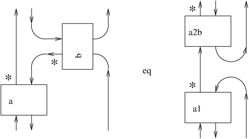
Note that $SF(a)=\delta^{-1}\phi_{1}(a)S\phi_{2}$ and $SF(b)=\delta^{-1}\widetilde{\phi}_{1}(a)S\widetilde{\phi}_{2}$, where $\widetilde{\phi}$ is another copy of $\phi$. Then the labelled tangle on the left of Figure 18 equals (by application of the (A) and (E) relations in $P(H^{*},\delta)$) either of the labelled tangles in Figure 19.

Figure 19. Simplifying the tangle on the left of Figure 18

We now simplify:

$$\delta^{-2}\phi_{1}(a)\widetilde{\phi}_{1}(b)S\widetilde{\phi}_{2}\otimes\widetilde{\phi}_{3}S\phi_{2} = \delta^{-2}(\phi_{1}\widetilde{\phi}_{3})(a)\widetilde{\phi}_{1}(b)S\widetilde{\phi}_{2}\otimes S\phi_{2}$$

$$= \delta^{-2}(\phi_{1}\widetilde{\phi}_{1})(a)\widetilde{\phi}_{2}(b)S\widetilde{\phi}_{3}\otimes S\phi_{2}$$

$$= \delta^{-2}\phi_{1}(a_{1})\widetilde{\phi}_{1}(a_{2})\widetilde{\phi}_{2}(b)S\widetilde{\phi}_{3}\otimes S\phi_{2}$$

$$= \delta^{-2}\phi_{1}(a_{1})\widetilde{\phi}_{1}(a_{2}b)S\widetilde{\phi}_{2}\otimes S\phi_{2}$$

$$= \delta^{-1}\widetilde{\phi}_{1}(a_{2}b)S\widetilde{\phi}_{2}\otimes\delta^{-1}\phi_{1}(a_{1})S\phi_{2}$$

$$= SF(a_{2}b)\otimes SF(a_{1})$$

where the first equality is a consequence of $\phi_{1}\otimes\psi S\phi_{2}=\phi_{1}\psi\otimes S\phi_{2}$ and the second is a consequence of the traciality of $\phi$.

Comparing the initial and terminal expressions in the above chain of equalities with the labelled tangles on the right in Figures 19 and 18 completes the proof. $\Box$

We conclude with the following corollary.

Corollary 14.

Suppose that $N$ is a planar network with $g$ boxes all of which are $2$-boxes. Then,

$$Z^{P(H,\delta)}_{N}=Z^{P(H^{*},\delta)}_{N^{-}}\circ F^{\otimes g},$$

where both sides are regarded as ${\bf k}$-valued functions on $H^{\otimes g}$.

Proof.

Note first that since $P(H,\delta)_{0_{\pm}}$ and $P(H^{*},\delta)_{0_{\pm}}$ are identified canonically with ${\bf k}$, the planar algebra isomorphism of Theorem 13, which maps ${}^{-}P(H,\delta)_{0_{\pm}}=P(H,\delta)_{0_{\mp}}$ to $P(H^{*},\delta)_{0_{\pm}}$, is identified with the identity map of ${\bf k}$.

According to Theorem 13, if $N$ is a planar network with $g$ boxes all of which are $2$-boxes, then, with the identifications above, $Z^{{}^{-}P(H,\delta)}_{N}=Z^{P(H^{*},\delta)}_{N}\circ(SF)^{\otimes g}$. But by definition, the former is $Z^{P(H,\delta)}_{N^{-}}$ while the latter is nothing but $Z^{P(H^{*},\delta)}_{N^{--}}\circ(F)^{\otimes g}$, since (i) $N^{--}=N\circ_{(B_{1},\cdots,B_{g})}(R_{2},\cdots,R_{2})$ where $R_{2}$ is the $2$-rotation tangle and (ii) $Z^{P(H^{*},\delta)}_{R_{2}}=S$. Now, replacing $N^{-}$ by $N$ yields the desired conclusion. $\Box$

7. appendix: tilings and tangles

This brief appendix will be devoted to a statement of a result in combinatorial topology and a sketch of its application in proving a generalisation of Lemma 6. We omit all proofs.

Consider a convex $2k$-gon in the plane with its vertices numbered from $1$ to $2k$ in clockwise order. By a tiling (by quadrilaterals) of the $2k$-gon we will mean a collection of its diagonals that are required to be non-intersecting and divide the polygon into quadrilaterals.

By a hexagon move on a tiling of a $2k$-gon, we will mean the following. Take two of its quadrilaterals that share an edge and consider the hexagon formed by their remaining edges. The common edge is a principal diagonal of this hexagon. Replace this principal diagonal with one of the other two principal diagonals of the hexagon to get a new tiling of the $2k$-gon.

Proposition 15.

Any two tilings of a $2k$-gon are related by a sequence of hexagon moves. $\Box$

The point of this digression into tilings and hexagon moves is roughly that tilings of a $2k$-gon correspond to tangles in ${\mathcal{T}(k)}$ (modulo the equivalence relation that forgets the internal $*$’s) while hexagon moves correspond to applying the exchange relations (E) and (A). Figure 20 shows some elements of ${\mathcal{T}}(3)$ and their corresponding tilings of the hexagon.

Figure 20. Some tangles and their associated tilings

Proposition 15 is the main step in the following generalisation of Lemma 6.

Lemma 16.

For each $k\geq 3$, and each $X\in{\mathcal{T}}(k)$, the map $Z^{P}_{X}:P_{2}^{\otimes(k-1)}\rightarrow P_{k}$ is surjective. $\Box$

References

- [DasKdy] Paramita Das and Vijay Kodiyalam, Planar algebras and the Ocneanu-Szymanski theorem, Proc. AMS, 133, (2005) 2751-2759.
- [Jns] V. F. R. Jones, Planar algebras I, New Zealand J. of Math., to appear. e-print arXiv: math.QA/9909027
- [KdyLndSnd] Vijay Kodiyalam, Zeph Landau and V. S. Sunder, The planar algebra associated to a Kac algebra, Proc. Indian Acad. of Sciences, 113, (2003) 15-51.
- [KdySnd] Vijay Kodiyalam and V. S. Sunder, On Jones’ planar algebras, J. Knot theory and its ramifications, 13, (2004) 219-247.
- [Lnd] Zeph Landau, Exchange Relation Planar Algebras, Proceedings of the Conference on Geometric and Combinatorial Group Theory, Part II (Haifa, 2000). Geom. Dedicata 95 (2002), 183–214.
- [LndSnd] Zeph Landau and V.S. Sunder, Planar depth and planar subalgebras, J. of Functional Analysis, 195, (2002), 71-88.
- [LrsRdf] R.G. Larson and D. E. Radford, Finite dimensional cosemisimple Hopf algebras in characteristic are semisimple, J. of Algebra, 117, 1988, 267–289.
- [Szy] Wojciech Szymanski, Finite index subfactors and Hopf algebra crossed products. Proc. Amer. Math. Soc. 120 (1994), 519528.
- [TngGlk] Pavel Etingof and Shlomo Gelaki, On finite-dimensional semisimple and cosemisimple Hopf algebras in positive characteristic. Internat. Math. Res. Notices 1998, 16, 851–864.