Virtual Knots and Links

Abstract

This paper is an introduction to the subject of virtual knot theory, combined with a discussion of some specific new theorems about virtual knots. The new results are as follows: We prove, using a 3-dimensional topology approach that if a connected sum of two virtual knots $K_{1}$ and $K_{2}$ is trivial, then so are both $K_{1}$ and $K_{2}$. We establish an algorithm, using Haken-Matveev technique, for recognizing virtual knots. This paper may be read as both an introduction and as a research paper.

For more about Haken-Matveev theory and its application to classical knot theory, see [Ha, Hem, Mat, HL].

1 Introduction

Virtual knot theory was proposed by Louis Kauffman in 1996, see [KaV]. The combinatorial notion of virtual knot is defined as an equivalence class of 4-valent plane diagrams (4-regular plane graphs with extra structure) where a new type of crossing (called virtual) is allowed.

This theory can be regarded as a “projection” of knot theory in thickened surfaces $S_{g}\times{\bf R}$ studied in [JKS]. Regarded from this point of view, virtual crossings appear as artifacts of the diagram projection from $S_{g}$ to ${\bf R}^{2}$. In such a virtual projection diagram, one does not know the genus of the surface from which the projection was made, and one wants to have intrinsic rules for handling the diagrams. The rules for handling the virtual diagrams were motivated in the first place (in [KaV]) by the idea that one can generalize the notion of a knot diagram to its oriented Gauss code. A Gauss code for a knot is list of crossings encountered on traversing the knot diagram, with the signs of the crossings indicated, and whether they are over or under in the course of the traverse. Each crossing is encountered twice in such a traverse, and thus the Gauss code has each crossing label appearing twice in the list. One can define Reidemeister moves on the Gauss codes, and thus abstract the knot theory from its planar diagrams. Virtual knot theory is the theory of such Gauss codes, not necessarily realizable in the plane. When one takes such a non-realizable code, and attempts to draw a planar diagram, virtual crossings are needed to complete the connections in the plane. These crossings are artifacts of the planar projection. It turns out that these rules describe embeddings of knots and links in thickened surfaces, stabilized by the addition and subtraction of empty handles (i.e. the addition and subtraction of thickened 1-handles from the surface that do not have any part of the knot or link embedded in them) [KaV2, KaV4, Ma1, Ma8, Ma10, CKS, KUP].

Another approach to Gauss codes for knots and links is the use of Gauss diagrams as in [GPV]). In this paper by Goussarov, Polyak and Viro, the virtual knot theory, taken as all Gauss diagrams up to Reidemeister moves, was used to analyze the structure of Vassiliev invariants for classical and virtual knots. In both [KaV] and [GPV] it is proved that if two classical knots are equivalent in the virtual category [KUP], then they are equivalent in the classical category. Thus classical knot theory is properly embedded in virtual knot theory.

To date, many invariants of classical knots have been generalized for the virtual case, see [GPV, KaV, KR, Ma1, Ma2, Ma8, Ma10, Saw, SW]. In many cases, a classical invariant extends to an invariant of virtual knots. In some cases one has an invariant of virtuals that is an extension of ideas from classical knot theory that vanishes or is otherwise trivial for classical knots. See [Saw],[SW], [KR], [Ma2, Ma3, Ma5]. Such invariants are valuable for the study of virtual knots, since they promise the possibility of distinguishing classical from virtual knots in key cases. On the other hand, some invariants evaluated on classical knots coincide with well known classical knot invariants (see [KaV, KaV2, KaV4, Ma3] on generalizations of the Jones polynomial, fundamental group, quandle and quantum link invariants). These invariants exhibit interesting phenomena on virtual knots and links: for instance, there exists a virtual knot $K$ with “fundamental group” isomorphic to ${\bf Z}$ and Jones polynomial not equal to $1$. This phenomenon immediately implies that the knot $K$ is not classical, and underlines the difficulty of extracting the Jones polynomial from the fundamental group in the classical case.

We know in principle that the fundamental group, plus peripheral information, determines the knot itself in the classical case. It is not known how to extract the Jones polynomial from this algebraic information. The formally defined fundamentaly group of a virtual knot can be interpreted as the fundamental group of the complement of the virtual knot in the one-point suspension of a thickened surface where this knot is presented.

Another phenomenon that does not appear in the classical case are long knots [Ma11]: if we break a virtual knot diagram at two different points and take them to the infinity, we may obtain two different long knots.

In the present paper, we are going to discuss both algebraic and geometric properties of virtual knots. We recommend as survey papers for virtual knot theory the following [DVK, Ma1, KUP, KaV4, KaV, FKM, FJK]

The paper is organized as follows. First, we give definitions and recall some known results. In the second section, we prove, using a 3-dimensional topology approach that if a connected sum of two virtual knots $K_{1}$ and $K_{2}$ is trivial, then so are both $K_{1}$ and $K_{2}$. Here we say “a connected sum” because the connected sum is generally not well defined. In the third section we introduce Haken-Matveev theory of normal surfaces in order to establish an algorithm for recognizing virtual knots. The fourth section is devoted to self-linking coefficient that generalizes the writhe of a classical knot. The fifth section is gives a quick survey of the relationship between virtual knots, welded knots and embeddings of tori in four-dimensional space.

We do not touch many different subjects on virtual knots. For instance, we do not describe virtual links and their invariatns. For more details see [Kam, Ver, FRR, Ma14, Ma12, KL].

1.1 Basic definitions

Let us start with the definitions and introduce the notation.

Definition 1.

A virtual link diagram is a planar graph of valency four endowed with the following structure: each vertex either has an overcrossing and undercrossing or is marked by a virtual crossing, (such a crossing is shown in Fig. 1).

Figure 1: Virtual crossing

All crossings except virtual ones are said to be classical.

Two diagrams of virtual links (or, simply, virtual diagrams) are said to be equivalent if there exists a sequence of generalized Reidemeister moves, transforming one diagram to the other one.

As in the classical case, all moves are thought to be performed inside a small domain; outside this domain the diagram does not change.

Definition 2.

Here we give the list of generalized Reidemeister moves:

1. Classical Reidemeister moves related to classical vertices.

2. Virtual versions $\Omega^{\prime}_{1},\Omega^{\prime}_{2},\Omega^{\prime}_{3}$ of Reidemeister moves, see Fig. 2.

   Figure 2: Moves $\Omega^{\prime}_{1},\Omega^{\prime}_{2},\Omega^{\prime}_{3}$

3. The “semivirtual” version of the third Reidemeister move, see Fig. 3,

   Figure 3: The semivirtual move $\Omega^{\prime\prime}_{3}$

Remark 1.

The two moves shown in Fig. 4 are forbidden, i.e., they are not in the list of generalized moves and cannot be expressed via these moves.

Figure 4: The forbidden move

Definition 3.

A virtual link is an equivalence class of virtual diagrams modulo generalized Reidemeister moves.

One can easily calculate the number of components of a virtual link. A virtual knot is a one–component virtual link.

Exercise 1.

Show that any virtual link having a diagram without classical crossings is equivalent to a classical unlink.

Remark 2.

Formally, virtual Reidemeister moves appear to give a new equivalence relation for classical links: there seem to exist two isotopy relations for classical links, the classical one that we are used to working with and the virtual one. Later we shall show that, for classical knots and links, virtual and classical equivalence are the same.

Remark 3.

Actually, the forbidden move is a very strong one. Each virtual knot can be transformed to any other one by using all generalized Reidemeister moves and the forbidden move.

This was proved by Sam Nelson in [Nel] (first mentioned in [GPV], see also [Kan]) by using Gauss diagrams of virtual links. Therefore, any two closed virtual knots are 1-equivalent and can be transformed to each other by a sequence of the Reidemeister moves and the forbidden moves.

If we allow only the forbidden move shown in the left part of Fig. 4, we obtain what are called welded knots, developed by Shin Satoh, [Satoh]. Some initial information on this theory can be found in [Kam], see also [FRR].

Definition 4.

By a mirror image of a virtual link diagram we mean a diagram obtained from the initial one by switching all types of classical crossings (all virtual crossings stay on the same positions).

1.1.1 Projections from handle bodies

The choice of generalized Reidemeister moves is very natural. It is the complete list of moves that occur when considering the projection of $S_{g}\times I$ to $R\times I$ (or equivalently $R^{3}$) in a generic projection of the thickened surface to the thickened plane. The virtual crossings appear in this projection as artifacts of different sheets of the surface being projected to the single sheet below. Actual crossings in the thickened surface are rendered as classical crossings in the thickened plane. The other moves, namely, the semivirtual move and purely virtual moves, are shown in Fig. 5 together with the corresponding moves in handle bodies.

Figure 5: Generalized Reidemeister moves and thickened surfaces

In fact, there exists a topological intepretation for virtual knot theory in terms of embeddings of links in thickened surfaces [KaV, KaV2]. Regard each virtual crossing as a shorthand for a detour of one of the arcs in the crossing through a $1$–handle that has been attached to the $2$–sphere of the original diagram. The two choices for the $1$–handle detour are homeomorphic to each other (as abstract manifolds with boundary). By interpreting each virtual crossing in such a way, we obtain an embedding of a collection of circles into a thickened surface $S_{g}\times{\bf R}$, where $g$ is the number of virtual crossings in the original diagram $L$ and $S_{g}$ is the orientable $2$–manifold homeomorphic to the sphere with $g$ handles. Thus, to each virtual diagram $L$ we obtain an embedding $s(L)\to S_{g(L)}\times{\bf R}$, where $g(L)$ is the number of virtual crossings of $L$ and $s(L)$ is a disjoint union of circles. We say that two such surface embeddings are stably equivalent if one can be obtained from the other by isotopy in the thickened surface, homeomorphisms of surfaces, and the addition of substraction or handles not incident to images of curves.

Theorem 1.

Two virtual link diagrams generate equivalent (isotopic) virtual links if and only if their corresponding surface embeddings are stably equivalent.

This result was sketched in [KaV]. The complete proof appears in [KaV3].

A hint to this prove is demonstrated in Fig. 5.

Here we wish to emphasize the following important circumstance.

Definition 5.

A virtual link diagram is minimal if no handles can be removed after a sequence of Reidemeister moves.

An important Theorem by Kuperberg [KUP] says the following.

Theorem 2.

For a virtual knot diagram $K$ there exists a unique minimal surface in which an $I$–neighbourhood of an equivalent diagram embeds and the embedding type of the surface is unique.

1.1.2 Gauss diagram approach

Definition 6.

A Gauss diagram of a (virtual) knot diagram $K$ is an oriented circle (with a fixed point) where pre-images of overcrossing and undercrossing of each crossing are connected by a chord. Pre-images of each classical crossing are connected by an arrow, directed from the pre-image of the overcrossing to the pre-image of the undercrossing. The sign of each arrow equals the local writhe number of the vertex. The signs of chords are defined as in the classical case. Note that arrows (chords) correspond only to classical crossings.

Remark 4.

For classical knots this definition is just the same as before.

Given a Gauss diagram with labelled arrows, if this diagram is realizable then it (uniquely) represents some classical knot diagram. Otherwise one cannot get any classical knot diagram.

Herewith, the four–valent graph represented by this Gauss diagram and not embeddable in ${\bf R}^{2}$ can be immersed to ${\bf R}^{2}$. Certainly, we shall consider only “good” immersions without triple points and tangencies.

Having such an immersion, let us associate virtual crossings with intersections of edge images, and classical crossings at images of crossing, see Fig. 6.

Figure 6: A virtual knot and its Gauss diagram

Thus, by a given Gauss diagram we have constructed (not uniquely) a virtual knot diagram.

Theorem 3 ([GPV]).

The virtual knot isotopy class is uniquely defined by this Gauss diagram.

Exercise 2.

Prove this fact.

Exercise 3.

Show that purely virtual moves and the semivirtual move are just the moves that do not change the Gauss diagram at all.

2 Underlying genus of virtual knots

The aim of this section is to prove the following.

Theorem 1.

Let $K_{1},K_{2}$ be two virtual knots. Then $g(K_{1}\#K_{2})\geq g(K_{1})+g(K_{2})-1$, whereas if $g(K_{1})=0$ or $g(K_{2})=0$ then $g(K_{1}\#K_{2})\geq g(K_{1})+g(K_{2})$.

From this theorem one can deduce the following

Theorem 2.

If $K_{1}$ and $K_{2}$ are virtual knots such that some connected sum $K_{1}\#K_{2}$ is trivial then both $K_{1}$ and $K_{2}$ are trivial knots.

Indeed, if at least one of $K_{1},K_{2}$ has positive underlying genus, then the underlying genus of their connected sum is also positive (by theorem 1). In the case when both knots have underlying genus zero, one should mention the following.

Lemma 1.

If $K_{1}$ and $K_{2}$ are two classical knots then any connected sum $K_{1}{\#}K_{2}$ of genus zero is equivalent to the (well-defined) classical connected sum $K_{1}{\#}K_{2}$.

This lemma follows directly from the proof of 1.

The remaining part of Theorem 2 now follows from the non-triviality of connected sum in the classical case, see, e.g. [CF].

2.1 Two types of connected sums

Having two virtual knots $K_{1}$ and $K_{2}$ represented by knots in thickened surfaces, there are two natural possibilities to represent their connected sum as a knot in a thickened surface.

The first way goes as follows. We take thickened surfaces $(M_{1}\times I)\supset K_{1}$ and $(M_{2}\times I)\supset K_{2}$ and cut two vertical full cylinders $D_{i}\times I$, where $D_{i}\subset M_{i}$, such that $D_{i}\cap K_{i}$ is homeomorphic to an interval. Then we paste these manifolds together (identifying $\partial D_{1}\times I$ and $\partial D_{2}\times I$ with respect to the orientation of manifolds and the direction of the interval $I$) and obtain $(M\times I)=((M_{1}\#M_{2})\times I)$ with $K_{1}\#K_{2}$ inside.

Clearly, $g(M)=g(M_{1})+g(M_{2})$.

Another way to construct the connected sum works only in some special cases. Suppose $K_{1}$ and $K_{2}$ lie in $M_{1}\times I,M_{2}\times I$, where both $g(M_{1})$ and $g(M_{2})$ are greater than zero, and there exist two non-trivial (non zero-homotopic) curves $\gamma_{1}\in M_{1}$ and $\gamma_{2}\in M_{2}$ such that $(\gamma_{i}\times I)\cap K_{i}$ consists of precisely one point (note that in this case such curve can not divide the $2$-manifold into two parts). Then we can cut $(M_{i}\times I)$ along $\gamma_{i}\times I$ and paste them together. Thus we obtain a manifold $M\times I$, where $g(M)=g(M_{1})+g(M_{2})-1$ with some connected sum $K_{1}\#K_{2}$ lying in $M$.

It turns out that these two connected sums are the only essential ways of connecting summation for virtual knots from which we deduce Theorem 2.

2.2 The proof plan of theorem 2

Consider two virtual knots $K_{1}$ and $K_{2}$ their connected sum $K_{1}\#K_{2}$. Let us realize this connected sum by curves in thickened surfaces by using the first method. Denote the corresponding surfaces by $M_{1},M_{2},M_{1}\#M_{2}$, and denote the corresponding knots by $K_{1},K_{2},K_{1}\#K_{2}$ (abusing notation). Now, we are going to transform $(M_{1}\#M_{2})\times I$ and knots inside it. We are going to check that the following condition holds during the transformation process (all notation stays the same during the transformation):

1. The ambient manifold $M$ is divided into two parts $M_{1}\#M_{2}$ such that $M_{i}\times I$ represents the knot $K_{i}$ (i.e., if we close this manifold, we obtain a surface realization of $K_{i}$).

2. The intersection $M=M_{1}\cap M_{2}$ consists of one or two components; so $(M_{1}\times I)\cap(M_{2}\times I)$ consists of one or two annuli.

3. The knot $K_{1}\#K_{2}$ intersects the manifold $(M_{1}\cap M_{2})$ precisely at two points; in the case when $M_{1}\cap M_{2}$ is not connected, these intersection points lie in different connected components.

4. The process stops when $g(M_{1}\#M_{2})$ is the minimal genus of the knot $K_{1}\#K_{2}$.

If we organize the process as described above, we prove Theorem 2. Indeed, at each moment of the process we have $K_{1}$ and $K_{2}$ represented by knots in thickened surfaces of genuses $g_{1}$ and $g_{2}$. The knot $K_{1}\#K_{2}$ lies in the surface of genus $g_{1}+g_{2}$ if we deal with the connected sum of the first type and in the surface of genus $g_{1}+g_{2}-1$ if we deal with the connected sum of the second type. So, the same holds when the process stops, thus we have $g(K_{1}{\#}K_{2})=g_{1}+g_{2}$ or $g(K_{1}{\#}K_{2})=g_{1}+g_{2}-1$, where the last case is possible only if we have the connected sum of the second type (hence, both $g_{1}$ and $g_{2}$ are greater than zero). Taking into account that $g_{i}$ is the genus of a surface (not necessarily minimal) representing $K_{i}$, we obtain the statement of the theorem.

2.3 The process

In the present subsection we describe how this process works.

Suppose we have the connected sum of type $i$ ($i=1$ or $2$) of the knots $K_{1}$ and $K_{2}$. The main statement is the following.

Statement 1.

If there is a possibility to decrease the genus of $M_{1}{\#}M_{2}$, then one of the following holds:

1. We can make a destabilization in $M_{i}$ without changing $M_{3-i}$ and the connected sum type (thus, we decrease the genus of one of connected summands $M_{i}$ by one, as well as that of $M_{1}{\#}M_{2}$).

2. If we have the connected sum of the first type, then there is a possibility to transform it to the connected sum of the second type decreasing the genus of $M_{1}{\#}M_{2}$ by one without changing the genuses of $M_{1}$ and $M_{2}$.

3. If we have the connected sum of the second type, then there is a possibility to transform it to the connected sum of the first type decreasing each of $g(M_{1}),g(M_{2}),g(M_{1}{\#}M_{2})$ by one.

Together with all described above, this statement completes the proof of Theorem 2.

Proof of Statement 1.

First, consider the case of the first type connected sum. We have $M=M_{1}{\#}M_{2}$. To simplify the notation, let us denote the corresponding manifolds with boundary by the same letter: $M=M_{1}{\#}M_{2}$, where $D=M_{1}\cap M_{2}$. Suppose we are able to destabilize the pair $((M_{1}{\#}M_{2})\times I,K_{1}{\#}K_{2}).$ Then there is a vertical annulus $C$ in $M_{1}{\#}M_{2}$ which does not intersect the knot $K_{1}{\#}K_{2}$. If there is such an annulus which does not intersect $D$, then we can destabilize one of the summands along $C$; this is the first case of Statement 1.

Suppose there is no such annulus $C$. Without loss of generality assume that the intersection between each such $C$ and $D$ is transverse. Let $n$ be the minimal number of connected components of the intersection $C\cap D$.

Since $C$ and $D$ are manifolds with boundary (vertical annuli), their intersection (in common position) may consist of:

1. simple circles;

2. trivial arcs;

3. horizontal circles;

4. vertical arcs;

Here the circle is trivial if it represent the trivial element in the fundamental group of the annulus $C$, otherwise the circle is called horizontal. The arc is called trivial if it connects points from the same boundary component of the annulus; otherwise it is called vertical.

If there is a simple circle then we can consider the innermost circle $\gamma$ (with respect to $C$). This circle contains no intersection points with $D$ inside. It is easy to see that there can be either none or two intersection points with the knot $K_{1}{\#}K_{2}$ because this circle together with a circle from $D$ bounds a sphere. In both these cases (with two intersections and with no intersections) we can slightly change the annulus $C$ in such a way that the total intersection between $C$ and $D$ decreases, and $C$ remains an essential annulus, see Fig. 7. The same situation happens when we have a trivial arc, see Fig. 8.

Figure 7: Non-horizontal discs in $A_{1}$

Figure 8: Removing the intersection along a non-vertical arc

Now, let us state two auxiliary lemmas.

Lemma 2.

Suppose $S_{g}$ is the oriented surface of genus $g$ and let $D$ be an embedded disc in $S_{g}$. Then if a closed non self-intersecting curve $\gamma\in S_{g}\backslash D$ is trivial in $S_{g}$ and not trivial in $S_{g}\backslash D$ then it is parallel to $\partial D$ (i.e. $D\cup S_{g}$ bounds a cylinder in $S_{g}$).

Indeed, if a curve $\gamma$ bounds a disk in $S_{g}$; which does not intersect $D$ then $\gamma$ is contractible in $S_{g}\backslash D$.

The following lemma is evident.

Lemma 3.

If an annulus $C^{\prime}$ is free homotopic to the annulus $D$ then $C^{\prime}$ intersects the knot $K_{1}{\#}K_{2}$.

Now, we may assume that our intersection $C\cap D$ consists only of vertical arcs or only of horizontal circles (the existence of a vertical arc contradicts the existence of a horizontal circle).

Suppose we have only horizontal circles. Then $C$ is homotopic to $D$ and, by Lemma 3, the annulus $C$ intersects the knot $K_{1}{\#}K_{2}$. Thus we obtain a contradiction.

Now, suppose the intersection $C\cap D$ consists only of vertical arcs. Then the annulus $C$ is divided into $2k$ parts $C_{1},\dots,C_{2k}$, whereas $C_{2l+1}$ lies in $M_{1}\times I$, and $C_{2l}$ lies in $M_{2}\times I$.The annulus $C\cap D$ is divided into $2k$ sectors by radii; some of these sectors contain intersection(s) with the knot, see Fig. 9. Denote these radii by $r_{1},\dots,r_{2k}$.

Figure 9: The annulus $C$ divided into sectors

Now, each part $C_{i}$ of the annulus $C$ is incident to two radii $r_{j}$ and $r_{k}$. Then $D$ is divided into two parts $D_{jk}^{+}$ and $D_{jk}^{-}$ by these radii. There are four options with respect to the following questions:

1. Does one of $D_{jk}^{+}$ and $D_{jk}^{-}$ contain any intersection with the knot?

2. Does the annulus obtained by attaching $C_{i}$ to one of $D_{jk}^{+}$ or $D_{jk}^{-}$ bound a ball (so that if we attach the other part, we obtain the annulus homotopic to $D$)?

Remark 5.

Here we mean that a proper surface (say, annulus) $F\subset M$ bounds a ball if $M\backslash F$ has two connected component, one of which is a topological ball. In other words, $F$ bounds a ball together with a part $P$ of boundary of the manifold $M$, so that $P\cup F$ is a sphere.

If both answers are affirmative: we obtain a contradiction: the intersection of a knot with a ball can not consist of only one point; if there are two such points, then of the knots $K_{1},K_{2}$ has underlying genus $0$, since it lies in a ball.

If the answer to the first question is negative and the answer to the second question is affirmative, we may easily decrease the number of connected components in $C\cap D$: we just “remove $C_{i}$” by pushing it through $D$. This is possible because $C_{i}\cup D$ bounds an empty ball.

If both answers are affirmative, then we can destabilize one of $(K_{i},M_{i})$ for $i=1,2$ along $C_{i}\cup D_{jk}^{+}$ (or along $C_{i}\cup D_{jk}^{-}$).

Finally, if ,say, $D_{jk}^{+}$ contains precisely one intersection with the knot then the number of intersection components of $C\cap D$ should be equal to two. If it is greater than two, then it can be decreased as shown in Fig. 10. More precisely, inside all parts $C_{i}$ of the annulus $C$ we take only two parts and compose a nontrivial annulus $C^{\prime}$, along which $(M_{1}\#M_{2})\times I$ with the knot $K_{1}{\#}K_{2}$ inside can be destabilized.

In other words, having more than two components $C_{i}$, one can find two of them which can be repasted and thus obtain a new non-trivial annulus $C^{\prime}$ intersecting $D$ at a smaller number of points.

Figure 10: Simplifying the curve $C$

Thus we see that if the intersection $C\cap D$ were minimal, there were precisely two connected components.

Let us show now that the destabilization along such $C$ just transforms the type of connected sum: we obtain a connected sum of the second type.

Indeed, the disc $D$ is just cut into two parts by this destabilization; and two intersection point after the destabilization lie in different connected components.

The proof for the case when we have the connected sum of the second type goes in the same vein. ∎

3 Algorithmical recognition of virtual links

The aim of this section is to prove the following

Theorem 3.

There is an algorithm to decide whether two virtual links are equivalent or not.

This theorem was first proved in [MaProof], see also [Ma12].

We shall use the result by Moise [Moi] that all 3-manifolds admit a triangulation. In the sequel, each 3-manifold is thought to be tringulated.

We shall deal with 3-manifolds (possibly, with boundary) and 2-surfaces in these manifolds. A compact surface $F$ in a manifold $M$ is called proper if $F\cap\partial M=\partial F$. In the sequel, all surfaces are assumed to be proper. A proper 2-dimensional submanifold in a 3-manifold is essential, if it does not cut a ball. We are interested in essential spheres, essential disks and essential annuli $S^{1}\times I$.

A mainfold $M$ is irrreducible if each embedded sphere in $M$ bounds a ball in $M$.

We shall use the definition of virtual knots as knots in thickened surfaces ${\cal M}\times I$ up to stabilizations/destabilizations. Here ${\cal M}$ is a compact 2-surface, not necessarily connected. Herewith we require that for each connected component ${\cal M}_{i}$, the 3-manifold ${\cal M}_{i}\times I$ contains at least one component of the link $L$.

Recall that a representative for a virtual link is minimal if it can not be destabilized.

We shall need the Kuperberg theorem [KUP] that says that the minimal representative $({\cal M}\times I,L)$ for each given link is unique up to isotopy.

Thus, in order to compare virtual links, we should be able to find their minimal representative and compare them. The algorithm to be given below uses a recognition techniques for three-manifolds with boundary pattern (see definition below) connected to virtual links in question.

We shall use the following facts from Haken-Matveev theory, see [Mat1].

A compressing disk for a surface $F$ in a $3$-manifold $M$ is an embedded disk $D\subset M$ which meets $F$ along its boundary, i.e. $D\cap F=\partial D$. A surface is called incompressible if it does not admit essential compressing disks.

A $3$-manifold is called irreducible if each $2$-sphere in it bounds a ball.

Let $D$ be a surface in a $3$-manifold $M$. An embedded disk $D\subset M$ is called a boundary compressing disk for $F$ if $D\cap F$ is a proper arc $l\in\partial D$, and $D\cap\partial M$ is the remaining arc of $\partial D$. Such disk is inessential if it cuts off a disk $D^{\prime}$ from $F$ so that $\partial D^{\prime}$ consists of a copy of $l$ and an arc on $\partial M$.

A surface $F\subset M$ is called boundary incompressible if it does not admit essential boundary compressing disks.

Also, a 3-manifold $M$ is boundary irreducible if any proper disk $D\subset M$ bounds a disk on $\partial M$.

Given a 3-manifold with boundary. By a boundary pattern (first proposed by Johannson, see [Joh]) we mean a fixed $1$–polyhedron (graph) without isolated points on the boundary of the three manifolds (we assume this graph be a subpolyhedron of the selected triangulation).

The existence of a boundary pattern does not change the definition of incompressible surface and irreducible manifolds.

We have straightforward generalizations of boundary incompressible surface and boundary irreducible manifold according to what is given below. A disk $D\subset M$ is called clean if it does not intersect the pattern.

Let $F$ be a surface in a manifold $(M,\Gamma)$. From now on, an essential boundary compressing disk for $F$ should be such that its boundary part lying on $\partial M$ is clean. This is the only novelty in the definition of boundary incompressible manifolds.

In the sequel, all proper surfaces with boundary are assumed to be clean.

Recall that an orientable 3-manifold $M$ is sufficiently large if it contains a proper incompressible boundary incompressible surface distinct from $S^{3}$ and ${\bf R}^{3}$.

A $3$-manifold without boundary (thus, without boundary pattern) is Haken if it is irreducible, boundary irreducible and sufficiently large. An irreducible boundary irreducible $3$-manifold $(M,\Gamma)$ with a boundary patteen $\Gamma$ is Haken either if it is sufficiently large or if its pattern $\Gamma$ is nonempty (hence, so is $\partial M$), and $M$ is a handlebody but not a ball.

We shall use the following

Proposition 1 ([Mat1]).

Any irreducible boundary irreducible 3-manifold with nonempty boundaryis either sufficiently large or a handle body.

Later on, we deal with manifolds with non-empty boundary pattern. For this manifold to be Haken, it is sufficient to check that it is irreducible and boundary irreducible but not a ball.

Lemma 4.

[Mat1] There exists an algorithm to decide whether a manifold $M$ is reducible; if it is so, the algorithm constructs a $2$-shere $S\subset M$ not bounding a ball in $M$.

Lemma 5.

[Mat1] Classical links are algorithmically recongizable.

This lemma follows from Haken’s theory of normal surfaces; the proof is based on the following ideas: for each non-trivial non-split link, the complement in $S^{3}$ to the tubular neighborhood of this link is a Haken manifold. Endowing the boundary with a pattern, we will be able to restore the initial link. After that, the problem is reduced to the recognition problem for Haken manifolds, for details see [Mat1].

Lemma 6.

[Mat1] There is an algorithm to decide whether a Haken manifold $M$ with a boundary pattern $\Gamma\subset\partial M$ has a propre clean essential annulus. If such an annulus exists, it can be constructed algorithmically.

We shall use this lemma to define whether some representative of a virtual link can be destabilized.

Lemma 7.

[Mat1] There is an algorithm to decide, whether two Haken manifolds $(M,\Gamma)$ and $(M^{\prime},\Gamma^{\prime})$ with boundary patterns are homeomorphic by means of a homeomorphism that maps $\Gamma$ to $\Gamma^{\prime}$.

Consider an arbitrary representative of a virtual link $L$, i.e., a couple $(M,L)$, where $M={\tilde{M}}\times I$ for some closed 2-surface ${\tilde{M}}$, and $L$ is a link in $M$ (we use the same letter $L$ for denoting both the initial link and the representing link in $M$: abusing notation). Let $N$ be a small open tubular neighborhood of the link $L$. Cut $N$ from $M$. We obtain a manifold with boundary. Denote it by $M_{L}$. Its boundary consists of boundary components of $M$ (two, if $M$ is connected) and several tori; the number of tori equals the number of components of the link $L$. Let us endow each torus with a pattern $\Gamma_{L}$, representing the meridian of the corresponding component (we also add a vertex to make a graph from the meridional circle). Thus we obtain the manifold $(M_{L},\Gamma_{L})$ with a boundary pattern.

It is obvious that the virtual link $L$ (and the pair $(M,L)$) can be restored from $(M_{L},\Gamma_{L})$, since we know how to restore the manifold $M$ by attaching full tori to the boundary components of $M_{L}$ knowing meridians of these full tori.

Lemma 8.

Suppose a link $L$ is not a split sum of a (nonempty) classical link and a virtual link Then the manifold $(M_{L},\Gamma_{L})$ with boundary pattern $\Gamma_{L}$ is Haken.

Proof.

In virtue of proposition 1, it remains to show that this manifold is irreducible and irreducible: it can not be a handlebody. ñ ðó÷êàìè.

Let $g=0$. Then, for any connected orientable $2$-surface $S_{g}$ the manifold $S_{g}\times I$ is irreducible. In the case when $g=0$ we deal with classical links. Thus, if the link $L$ is not classical then for its neighborhood $N(L)$, the set $(S_{g}\times I)\backslash N(L)$ might be reducible if and only if it contains a sphere $S$, bounding a ball in $S_{g}\times\{0,1\}$ such that this ball contains some components of the link $L$. This means that these components form a classical sublink of $L$ separated from all other components.

Furthermore, since $L$ is not a split sum of the unknot with some virtual link, the manifold $M_{L}$ is boundary irreducible.

Indeed, each curve in $S_{g}\times\{0\}$ or in $S_{g}\times\{1\}$ which may bound a disk in $S_{g}\times I$ is contractible in the boundary. Thus, boundary reducibility might occur only if we have a proper disk with boundary lying on some torus — the boundary of the cut full torus. This should mean that the cut full torus corrsponds to the split unknot of the link.

Thus, the considered manifold is irreducible and boundary irreducible and thus (by proposition 1), Haken. ∎

From what above we obtain the following

Lemma 9.

Let $L$ be a virtual link that can not be presented as split sum $K\cup L^{\prime}$ of a classical link $K$ and a virtual link $L^{\prime}$. Then the manifold $M_{L}$ is irreducible.

Now, let us prove the main theorem. Let $L,L^{\prime}$ be virtual links.

1. Consider some representatives $(M,L),(M^{\prime},L^{\prime})$ of the virtual links in question. Let us construct the corresponding manifolds with boundary patterns. Denote them by $(M_{L},\Gamma),(M^{\prime}_{L^{\prime}},\Gamma^{\prime})$.

2. Define whether one of $M_{L}$ or $M^{\prime}_{L^{\prime}}$ is reducible. If one of them is so, then, by lemma 4, we may find a sphere not bounding a ball, and thus separate some classical components of the corresponding link.

3. Define (by lemma 6) whether it is possible to destabilize one of the surfaces $(M_{L},\Gamma)$ or $(M^{\prime}_{L^{\prime}},\Gamma^{\prime})$. If it is possible, perform the destabilization. Return to step 2.

   Let us perform steps 2 and 3 while possible. Obviously, this process stops in a finite period of time.

   Classical links are algorithmically recognizable. Thus, we may compare the split classical sublinks of $L$ and $L^{\prime}$. If they are not isotopic, we stop: the virtual links in question are not equivalent. Otherwise, we go on.

   After performing the first three steps, we reduce our problem to the case when there are no split components and representatives are minimal. From now on, the manifolds in question are Haken by lemma 9.

4. Each connected component of the manifolds $(M_{L},\Gamma)$ and $(M^{\prime}_{L^{\prime}},\Gamma^{\prime})$ is a Haken manifold with a boundary pattern. Thus, we can algorithmically solve the problem whether there exists a homeomorphism $f:M_{L}\to M^{\prime}_{L^{\prime}}$ that maps $\Gamma$ to $\Gamma^{\prime}$ (ïî ëåììå 7). If such a homeomorphism exists then virtual links $L,L^{\prime}$ are equivalent. Otherwise $L$ and $L^{\prime}$ are not equivalent.

Performing the steps described above, we solve the recognition problem. Theorem is proved.

Remark 6.

The proof given below works also for oriented virtual links and framed virtual links.

4 Self-linking Numbers for Virtual Links

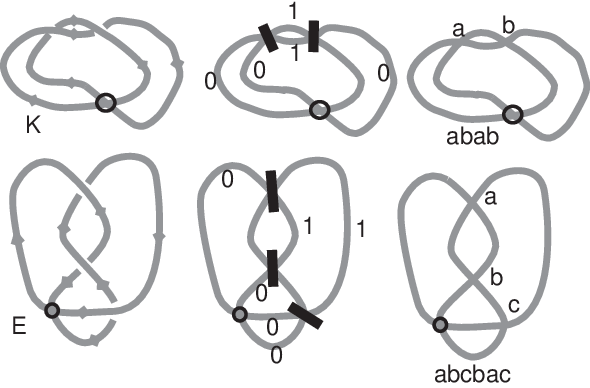
Call a crossing You mean a classical crossing, don’t you? in an oriented virtual knot diagram $K$ odd if, in the Gauss code for that diagram there are an odd number of appearances of (classical) crossings between the first and the second appearance of $i.$ Let

$$J(K)=w(K)|_{Odd(K)}$$

where $Odd(K)$ denotes the collection of odd crossings of $K,$ and the restriction of the writhe to $Odd(K)$, $w(K)|_{Odd(K)},$ means the summation over the signs of the odd crossings in $K.$ Then it is not hard to see that $J(K)$ is invariant of the virtual knot or link $K.$ We call $J(K)$ the self-linking number of the virtual diagram $K.$ This invariant is simple, but remarkably powerful.

Theorem. If $K$ is classical then $J(K)=0,$ since there are no odd crossings in a classical diagram. Note that if $K$ is a virtual knot and $K^{*}$ denotes the mirror image of $K$ (obtained by switching all the crossings of the diagram $K$), then

$$J(K^{*})=-J(K).$$

Hence, if $J(K)$ is non-zero, then $K$ is inequivalent to its mirror image. If K is a virtual knot and $J(K)$ is non-zero, then $K$ is not equivalent to a classical knot.

We leave the proof of this Theorem and the proof of the invariance of $J(K)$ to the reader. See [SelfLink] for more about this invariant its generalizations.

View Figure . The two virtual knots in this figure illustrate the application of Theorem 2. In the case of the virtual trefoil $K,$ the Gauss code of the shadow of $K$ is $abab;$ hence both crossings are odd, and we have $J(K)=2.$ This proves that $K$ is non-trivial, non-classical and inequivalent to its mirror image. Similarly, the virtual knot $E$ has shadow code $abcbac$ so that the crossings $a$ and $b$ are odd. Hence $J(E)=2$ and $E$ is also non-trivial, non- classical and chiral. Note that for $E,$ the invariant is independent of the type of the even crossing $c.$

Figure 11: Virtual Trefoil $K$ and Virtual Figure Eight $E$

5 Welded Braids and Tubes in Four-Space

The welded braid group $WB_{n}$ can be interpreted as the fundamental group of the configuration space of $n$ disjoint circles trivially embedded in three dimensional space $R^{3}$. This group (the so-called motion group of disjoint circles) can, in turn, be interpreted as a braid group of tubes imbedded in $R^{3}\times R=R^{4}.$ These braided tubes in four-space are generated by two types of elementary braiding. In Figure 12, we show diagrams that can be interpreted as immersions of tubes in three-space. Each such immersion is a projection of a corresponding embedding in four-space. The first two diagrams of Figure 12 each illustrate a tube passing through another tube. When tube $A$ passes through tube $B$ we make a corresponding classical braiding crossing with arc $A$ passing under arc $B.$ The four-dimensional interpretation of tube $A$ passing through tube $B$ is that: As one looks at the levels of intersection with $R^{3}\times t$ for different values of $t,$ one sees two circles $A(t)$ and $B(t).$ As the variable $t$ increases, the $A(t)$ circle (always disjointly embedded from the $B(t)$ circle) moves through the $B(t)$ circle. This process is illustrated in Figure 13.

While the classical crossing in a welded braid diagram corresponds to a genuine braiding of the tubes in four-space (as described above), the virtual crossing corresponds to tubes that do not interact in the immersion representation (see again Figure 12). These non-interacting tubes can pass over or under each other, as these local projections correspond to equivalent embeddings in four-space.

Figure 12: Tubular correspondence

Figure 13: Braiding of circles

It is an interesting exercise to verify that the moves in the welded braid group each induce equivalences of the corresponding tubular braids in four-space. In particular, the move $(F_{1})$ induces such an isotopy, while the forbidden move $(F_{2})$ does not. For more on this subject, the reader can consult [Satoh] and also [DVK] and the references therein. The basic idea for this correspondence is due to Satoh in [Satoh] where torus embeddings in four-space are associated with virtual knot diagrams.

Consider now the surjection $WB_{n}\longrightarrow FU_{n}$ from the welded braid group to the flat unrestricted braids. Flat unrestricted braids can be represented by immersions of tubes in three-space as illustrated also in Figure 12. There we have indicated a decorated immersion of two intersecting tubes as the correspondent of the flat classical crossing in $FU_{n}.$ One must specify the rules for handling these immersions in order to obtain the correspondence. We omit that discussion here, but point out the interest in having a uniform context for the surjection of the welded braids to the flat unrestriced braids. The flat unrestricted braids carry the distinction between braided flat and welded flat crossings and otherwise keep track of the relative permutations of these two types of crossing.

For knot theory the moral of these remarks is that the category of welded knots and links (virtual knots and links plus the equivalence relation generated by the first forbidden move) is naturally associated with embeddings of tori in four dimensional space. To each welded knot or link there is associated a well-defined embedding of a collection of tori (one torus for each component of the given link) and the fundamental group of the complement of this embedding in four space is isomorphic to the combinatorial fundamental group of the welded link (this is the same as the combinatorial fundamental group of a corresponding virtual link). It is an open problem whether this association is am embedding of the category of welded links into the category of tororidal embeddings in four-space.

References

- [BF] Bartholomew, A. and Fenn R. (2003), Quaternionic Invariants of Virtual Knots and Links, www.maths.sussex.ac.ukStaffRAFMathsCurrentAndyequivalent.ps
- [CF] Crowell, R.H., Fox, R.H. (1963), Introduction to knot theory, (New York: Ginn & Co).
- [CS] J.S.Carter and M. Saito, Diagrammatic invariants of knotted curves and surfaces, (unpublished manuscript - 1992).
- [CKS] J. S. Carter, S. Kamada and M. Saito, Stable equivalence of knots on surfaces and virtual knot cobordisms. arXiv:math.GT/0008118 v1 16 Aug 2000, J. Knot Theory & Ramifications, 11 (2002), Vol.3, pp. 311-322.
- [Dyn] E.B.Dynkin, On the Coefficients in Campbell–Hausdorff formula, Doklady Mathematics, Vol.57, N. 4, pp.323–326 (1947).
- [FJK] R. A. Fenn, M. Jordan and L. H. Kauffman (2004), Biquandles and Virtual Links, Topology and Its applications, bf 145, pp. 157-175.
- [FKM] R. A. Fenn, L. H. Kauffman and V. O. Manturov, Virtual Knots, Unsolved Problems, to appear in Selecta Mathematica: Proceedings of ”Knots in Poland-2003” Conference.
- [GPV] Goussarov M., Polyak M., and Viro O.(2000), Finite type invariants of classical and virtual knots, Topology 39, pp. 1045–1068.
- [Ha] Haken, W. (1961), Theorie der Normalflächen, Acta Mathematicae 105, pp. 245–375.
- [Hem] Hemion, G. (1992), The classification of knots and 3–dimensional spaces, (Oxford: Oxford Univ. Press).
- [HL] Hass, J., Lagarias, J. (2001), The number of Reidemeister moves needed for unknotting, J. Amer. Math. Soc., 14 (2), pp. 399-428.
- [HK] Hrencecin, D. and Kauffman, L.H., On Filamentations and Virtual Knots, Topology and its Applications, 134, pp. 23–52.
- [Joh] Johansson, K.(1979), Homotopy equivalences of -manifolds with boundaries, Lecture Notes in Mathematics, 761, (Berlin: Springer-Verlag).
- [Joy] Joyce, David (1983), The classifying invariant of knots, the knot quandle, Journal of Pure and Applied Algebra, 23 (1), pp. 37–65.
- [Kad] Kadokami, S. (2003), Detecting non-triviality of virtual links, Journal of Knot Theory and Its Ramifications, 6, pp. 781-819.
- [Kam] Kamada, S. (2000), Braid presentation of virtual knots and welded knots, arXiv:math. GT/0008092 v1, 2000.
- [Kan] Kanenobu, T (2001), Forbidden moves unknot a virtual knot, Journal of Knot Theory and Its Ramifications, 10 (1), pp. 89-96.
- [Kau0] Kauffman, L.H., “Virtual Knot Theory”, Talk at the AMS Meeting, January, 2000.
- [KNOTS] Louis H. Kauffman, Knots and Physics, World Scientific, Singapore/New Jersey/London/Hong Kong, 1991, 1994, 2001.
- [KL] L.H. Kauffman, S. Lambropoulou, Virtual braids and the L-move, to appear in Fundamenta Mathematica.
- [KaV] Kauffman, L. H. (1999), Virtual knot theory, European Journal of Combinatorics, 20(7), pp. 662-690.
- [KaV2] Kauffman, L.H., Detecting virtual knots, Atti. Sem. Math. Fis., Univ. Modena, Supplemento al Vol. IL, 241-282 (2001). YOU HAVE THIS APPEARING ALSO AS ”DVK” IN THIS BIBLIOGRAPHY!
- [KaV3] Kauffman, L.H.., Diagrammatic Knot Theory (in Preparation).
- [KaV4] H. Dye and L. H. Kauffman, Minimal surface representations of virtual knots and links. arXiv:math.AT/0401035 v1, Jan. 2004.
- [SelfLink] L. H. Kauffman, A Self-Linking Invariant of Virtual Knots. (to appear in Fundmentae Mathematicae).
- [Kim] Kim, S.G. ((1999), Virtual Knot Groups, arXiv:math.GT/9907172, 1,Journal of Knot Theory and Its Ramifications, 9(6), 2000.
- [KR] Kauffman, L.H. and Radford, D. (2002), Bi–Oriented Quantum Algebras, and Generalized Alexander Polynomial for Virtual Links, AMS. Contemp. Math.,318, pp. 113–140.
- [KS] Kishino, T., Satoh, S., A note on non-classical virtual knots. b
- [JKS] Jaeger, F., Kauffman, L.H. and Saleur, H. (1994), The Conway Polynomial in and Thickened Surfaces: A new Determinant Formulation, J. Combin. Theory. Ser. B., 61, pp. 237-259.
- [KUP] Greg Kuperberg, What is a virtual link? arXiv:math.GT/0208039 v1 5 Aug 2002,Algebraic and Geometric Topology, 2003, 3, 587-591
- [Ma1] Manturov, V.O. (2004), Knot Theory, (London: Chapman & Hall CRC Press).
- [Ma2] Manturov, V.O. (2002), On Invariants of Virtual Links, Acta Applicandae Mathematicae, 72 (3), pp. 295–309.
- [Ma3] Manturov, V.O. (2003), Multivariable polynomial invariants for virtual knots and links, Journal of Knot Theory and Its Ramifications,12,(8), pp. 1131-1144.
- [Ma4] Manturov, V.O. (2002), Virtual knots and infinite-dimensional Lie algebras, Acta Applicandae Mathematicae, submitted.
- [Ma5] Manturov, V.O. (2002), Invariants of Virtual Links, Doklady Mathematics, 65(3), pp. 329–331.
- [Ma6] Manturov, V.O. (2003), Curves on Surfaces, Virtual Knots, and the Jones–Kauffman Polynomial, Doklady Mathematics, 67(3), pp. 326–328.
- [Ma7] Manturov, V.O. (2002), Two–variable invariant polynomials for virtual links, Russian Math. Surveys, 57(5), pp. 997–998.
- [Ma8] Manturov V.O. (2003), Kauffman–like polynomial and curves in –surfaces, Journal of Knot Theory and Its Ramifications, 12,(8),pp.1145-1153.
- [Ma9] Manturov, V.O. (2003), Multivariable polynomial invariants for virtual knots and links, Journal of Knot Theory and Its Ramifications,12,(8), pp. 1131-1144
- [Ma10] Manturov, V.O. (2004), Vassiliev Invariants for Virtual Links, Curves on Surfaces and The Jones-Kauffman polynomial, Journal of Knot Theory and Its Ramifications, to appear.
- [Ma11] Manturov, V.O. (2004), Long virtual knots and their invariants, Journal of Knot Theory and Its Ramifications, 8.
- [Ma12] Manturov, V.O. (2005), Teoriya uzlov (Knot Theory), Regular and chaotic dynamics, Moscow-Izhevsk, 2005.
- [Ma13] Manturov, V.O.(2004), Virtual knots are algorithmically recognisable., arXiv:math. GT/0408255 v1.
- [Ma14] Manturov, V.O (2003), O raspoznavanii virtual’nykh kos, Zap. Nauchn. Seminarov POMI, 299. Geometriya i topologiya, 8, ññ. 267-286.
- [Moi] Moise, E.E. (1952), Affine structures in –manifolds. V. The triangulation theorem and Hauptvermutung, Annals of Mathematics, 57, pp. 547–560.
- [Mat] Matveev, S.V. (1984), Distributive grouppoids in Knot Theory, Mat. Sbornik, 47, pp.73–83.
- [Mat1] Matveev, S.V. (2003), Algorithmic topology and classification of 3-manifolds, (Springer Verlag).
- [Nel] Nelson, S. (2001), Unknotting virtual knots with Gauss diagram forbidden moves, Journal of Knot Theory and Its Ramifications, 10 (6), pp. 931–935.
- [FRR] R. Fenn, R. Rimanyi and C. Rourke, The Braid Permutation Group, Topology, Vol. 36, No. 1 (1997), 123–135.
- [Satoh] Shin Satoh, Virtual knot presentation of ribbon torus knots, J. knot theory & Ramifications, 9 (2000), pp. 531-542.
- [DVK] Louis H. Kauffman, Detecting Virtual Knots, Atti. Sem. Mat. Fis. Univ. Modena Supplemento al Vol. IL (2001), 241–282.
- [Saw] J. Sawollek, On Alexander-Conway polynomials for virtual knots and links, arXiv:math.GT/9912173 21 Dec 1999. J. Knot Theory Ramifications 12 (2003), no. 6, 767–779.
- [SW] D. S. Silver and S. G. Williams, Alexander Groups and Virtual Links, Journal of Knot Theory and Its Ramifications, 10 (1),pp. 151-160
- [Tur] V. G. Turaev, Virtual Strings, arXiv:math.GT/0310218, v1
- [VBOOK] Louis H. Kauffman, Vassily O. Manturov, Virtual Knot Theory, in preparation.
- [Ver] Vershinin, V. (2001), On Homology of Virtual Braids and Burau Representation, Journal of Knot Theory and Its Ramifications, 18(5), pp. 795–812.
- [W] S. Winker. PhD. Thesis, University of Illinois at Chicago (1984)