The first bifurcation point for Delaunay nodoids

Wayne Rossman

Abstract: We give two numerical methods for computing the first bifurcation point for Delaunay nodoids. With regard to methods for constructing constant mean curvature surfaces, we conclude that the bifurcation point in the analytic method of Mazzeo-Pacard is the same as a limiting point encountered in the integrable systems method of Dorfmeister-Pedit-Wu.

1. Introduction

Delaunay surfaces in Euclidean $3$-space

$$\mbox{$R$}^{3}=\{(x_{1},x_{2},x_{3})\,|\,x_{j}\in\mbox{$R$}\}$$

are constant mean curvature (CMC) surfaces of revolution, and they are translationally periodic. By a rigid motion and homothety of $\mbox{$R$}^{3}$ we may place the Delaunay surfaces so that their axis of revolution is the $x_{1}$-axis and their constant mean curvature is $H=1$ (henceforth we assume this).

We consider the profile curve in the half-plane $\{(x_{1},0,x_{3})\in\mbox{$R$}^{3}\,|\,x_{3}>0\}$ that gets rotated about the $x_{1}$-axis to trace out a Delaunay surface. This curve alternates periodically between maximal and minimal heights (with respect to the positive $x_{3}$ direction), which we refer to as the bulge radius and the neck radius, respectively, of the Delaunay surface. Let us denote the neck radius by $r$.

Delaunay surfaces come in two $1$-parameter families: one is a family of embedded surfaces called unduloids that can be parametrized by the neck radius $r\in(0,1/2]$; the other is a family of nonembedded surfaces called nodoids that can be parametrized by the neck radius $r\in(0,\infty)$. For unduloids, $r=1/2$ gives the round cylinder. For both unduloids and nodoids, the limiting singular surface as $r\to 0$ is a chain of tangent spheres of radii $1$ centered along the $x_{1}$-axis.

In this paper we shall be concerned with nodoids. We will see that a common bifurcation point for Delaunay nodoids is encountered in the following two distinctly different approaches for constructing CMC surfaces:

1. Using analytic techniques, Mazzeo and Pacard [15] showed existence of a finite value $r_{0}$ so that for neck radii $r<r_{0}$ the nodoids are nonbifurcating, and for $r>r_{0}$ the nodoids can bifurcate. Bifurcating nodoids are of interest because they deform smoothly through families of CMC surfaces that are of bounded distance from a fixed line yet are not surfaces of revolution. Before the work [15], such examples were unknown.

   To study this bifurcation, a particular Jacobi operator associated to the second variation formula for Delaunay surfaces is used, along with a function space that contains only functions with the same translational periodicity as the Delaunay surfaces themselves. Because these functions are translationally periodic, they do not have finite $L^{2}$ norms on the entirety of the surfaces. Hence bifurcation is a different notion from that of ”nondegeneracy” of CMC surfaces, i.e. CMC surfaces with no nonzero Jacobi fields of finite $L^{2}$ norm on the entire surfaces. However, the two notions have the common trait of being highly useful tools for producing previously unknown CMC surfaces. (There has been much work done related to the nondegeneracy of CMC surfaces and construction of new CMC examples, see for example the works of Kapouleas, Kusner, Mazzeo, Pacard, Pollack, Ratzkin [10], [11], [14], [16], [17], [21].) As our interest here is in the bifurcation of Delaunay nodoids, from the outset we consider only periodic functions on Delaunay surfaces.

   Mazzeo and Pacard gave a clear reason for the existence of this bifurcation point $r_{0}$, in terms of the existence of nontrivial nullity for the Jacobi operator, but they did not compute the precise value of $r_{0}$.

2. Using integrable systems techniques developed by Dorfmeister, Pedit and Wu in [8], Dorfmeister, Wu [9] and Schmitt [23] (see also [12]) constructed genus $0$ CMC surfaces with three asymptotically Delaunay ends. In [9] the construction was restricted to surfaces with asymptotically unduloidal ends, because such ends are embedded. However, the construction in [23] and [12] includes asymptotically nodoidal ends as well. The construction begins with the selection of a certain ”DPW potential”, and the DPW potential in [23] and [12] fails to exist when some nodoidal end has an asymptotic neck radius greater than $1/2$. Furthermore, the arguments in [23] and [12] showing that each end converges to a Delaunay surface work only when the limiting Delaunay surface is an unduloid, or is a nodoid with neck size less than $1/2$. This suggests that there is possibly some obstruction in the DPW approach to CMC surfaces with Delaunay ends that occurs only for asymptotically nodoidal ends with asymptotic neck radii at least $1/2$.

   In the construction in [23] and [12], this limiting value $1/2$ appears explicitly, but the underlying reasons for its appearance are left unexplained.

It is natural to ask if the bifurcation radius $r_{0}$ in the first approach coincides with the limiting value $1/2$ in the second approach. The purpose of this article is to numerically confirm this:

Numerical result. The bifurcation radius $r_{0}$ is equal to $1/2$.

This result is of interested with respect to both approaches above. For the first approach, it gives the exact (previously unknown) value for $r_{0}$. For the second approach, it provides a reason (via the bifurcation properties shown by Mazzeo and Pacard) for the existence of the previously mysterious limiting value $1/2$.

In fact, we shall show a stronger numerical result about the first eigenvalue of a particular operator, for which the above numerical result is an immediate corollary.

To provide added confidence in the accuracy of our numerical arguments, we give two different independent algorithms for showing that $r_{0}=1/2$ (and for showing the stronger numerical result as well). The first method involves using an ordinary differential equation (ODE) solver and symmetry properties of the first eigenfunction. The second method requires more machinery, the basic tool being the Rayleigh quotient characterization for eigenvalues of a self-adjoint operator. It involves numerical integration of smooth bounded functions of a single variable on a finite interval, and it has the advantage of also giving estimates for other eigenvalues beyond the first one.

2. Jacobi elliptic functions

Before introducing equations for nodoids in the next section, we first briefly review the properties of Jacobi elliptic functions needed here. For $\phi,k\in\mbox{$R$}$ with $0<k^{2}<1$, we set

(1) $$\xi=\int_{0}^{\phi}\frac{d\psi}{\sqrt{1-k^{2}\sin^{2}\psi}}\;,$$

and then we define

$$\text{sn}_{k}(\xi)=\sin\phi\;,\;\;\;\text{cn}_{k}(\xi)=\cos\phi\;,\;\;\;\text{dn}_{k}(\xi)=\sqrt{1-k^{2}\sin^{2}\phi}\;.$$

Extending these functions analytically to $\xi\in\mathbb{C}$, they are defined on the complex plane (with singularities). A short computation gives

(2) $$\frac{d}{d\xi}\text{sn}_{k}(\xi)=\text{cn}_{k}(\xi)\cdot\text{dn}_{k}(\xi)\;.$$

Defining

(3) $$z=\tilde{c}\cdot\text{sn}_{k}(\tilde{a}\xi+\tilde{b})$$

for constants $\tilde{a},\tilde{b}$ and $\tilde{c}$, Equation (2) then gives

(4) $$\frac{1}{z}\frac{dz}{d\xi}=\frac{\tilde{a}\cdot\text{cn}_{k}(\tilde{a}\xi+\tilde{b})\cdot\text{dn}_{k}(\tilde{a}\xi+\tilde{b})}{\text{sn}_{k}(\tilde{a}\xi+\tilde{b})}$$

and

(5) $$\left(\frac{dz}{d\xi}\right)^{2}+\tilde{a}^{2}(1+k)^{2}z^{2}-\tilde{a}^{2}(\tilde{c}+k\tilde{c}^{-1}z^{2})^{2}=0\;.$$

Let $\text{sn}^{-1}_{k}$ denote the (multi-valued) inverse function of $\text{sn}_{k}$. Although multi-valued, from here on out let us fix $\text{sn}^{-1}_{k}(1)$ to be equal to the specific value of $\xi\in\mbox{$R$}$ given by the integral (1) with $\phi=\pi/2$.

Lemma 1.

Suppose that $\tilde{b}=$sn${}^{-1}_{k}(1)$, and that $\tilde{c}>0$ and $\tilde{a}\in i\mbox{$R$}$. Then the function $z$ as in Equation (3) is positive (i.e. $z\in\mbox{$R$}^{+}$) and periodic with respect to the variable $\xi\in\mbox{$R$}$.

Proof.

Using the identity

$$\text{sn}_{k}(\tilde{u}+\tilde{v})=\frac{\text{sn}_{k}(\tilde{u})\text{cn}_{k}(\tilde{v})\text{dn}_{k}(\tilde{v})+\text{sn}_{k}(\tilde{v})\text{cn}_{k}(\tilde{u})\text{dn}_{k}(\tilde{u})}{1-k^{2}\text{sn}_{k}^{2}(\tilde{u})\text{sn}_{k}^{2}(\tilde{v})}$$

with $\tilde{u}=\tilde{a}\xi$ and $\tilde{v}=\tilde{b}$, we have

$$z=\tilde{c}\frac{\text{cn}_{k}(\tilde{a}\xi)}{\text{dn}_{k}(\tilde{a}\xi)}\;.$$

Then using the relations

$$\text{cn}_{k}(i\tilde{u})=\frac{1}{\text{cn}_{k^{\prime}}(\tilde{u})}\;,\;\;\;\text{dn}_{k}(i\tilde{u})=\frac{\text{dn}_{k^{\prime}}(\tilde{u})}{\text{cn}_{k^{\prime}}(\tilde{u})}$$

with $k^{\prime}\in\mbox{$R$}$ satisfying $(k^{\prime})^{2}+k^{2}=1$, we have

$$z=\frac{\tilde{c}}{\text{dn}_{k^{\prime}}(-i\tilde{a}\xi)}\;.$$

It follows that $z$ is positive and periodic when $\xi\in\mbox{$R$}$, because $-i\tilde{a}\xi\in\mbox{$R$}$ and $\text{dn}_{k^{\prime}}$ is positive and periodic with respect to a real variable. ∎

3. Parametrizing nodoids

Let $(x_{1},x_{2},x_{3})$ be the usual rectangular coordinates for $\mbox{$R$}^{3}$. Consider a Delaunay nodoid with the $x_{1}$-axis as its axis and with constant mean curvature $H=1$. Let

$$(x(t),z(t))\;,\;\;\;t\in\mbox{$R$}$$

be a parametrization of the profile curve of the nodoid in the $x_{1}x_{3}$-plane, and so the surface can now be parametrized by

$${\mathcal{D}}(t,\theta)=(x(t),z(t)\cos\theta,z(t)\sin\theta)\;,\;\;\;t\in\mbox{$R$}\;,\;\;\theta\in[0,2\pi)\;.$$

Suppose further that the parameter $t$ is chosen to make the mapping ${\mathcal{D}}(t,\theta)$ conformal with respect to the coordinates $(t,\theta)$. Let $t=a$ and $t=b$ be values at which the nodoid achieves two adjacent necks, i.e. $z(t)$ has local minima at both $t=a$ and $t=b$ equal to the neck radius $r$ but at no $t\in(a,b)$. Conformality implies that the first fundamental form is

$$ds^{2}=((x^{\prime})^{2}+(z^{\prime})^{2})dt^{2}+z^{2}d\theta^{2}=\rho^{2}(dt^{2}+d\theta^{2})\;,$$

with

$$\rho^{2}=(x^{\prime})^{2}+(z^{\prime})^{2}=z^{2}\;.$$

The second fundamental form is then

$$\tfrac{1}{z}(x^{\prime\prime}z^{\prime}-z^{\prime\prime}x^{\prime})dt^{2}+x^{\prime}d\theta^{2}\;,$$

and so the coordinates $(t,\theta)$ are curvature line coordinates, that is, the coordinates are isothermic. Furthermore, the mean curvature $H=1$ implies

$$2z^{3}-z^{\prime}x^{\prime\prime}+x^{\prime}z^{\prime\prime}-zx^{\prime}=0\;.$$

This has a first integral, that is, using $z^{2}=(x^{\prime})^{2}+(z^{\prime})^{2}$ and $zz^{\prime}=x^{\prime}x^{\prime\prime}+z^{\prime}z^{\prime\prime}$, it is equivalent to

$$(4x^{\prime}-4z^{2})^{\prime}=0\;.$$

Thus

(6) $$m=4x^{\prime}-4z^{2}$$

is satisfied for some $t$-independent constant $m$. Because there are points on a nodoid where $x^{\prime}=0$, we have

$$m<0\;.$$

In fact, $m\in(-\infty,0)$ is a parameter that determines the full family of Delaunay nodoids. Equation (6) can also be established using a homology invariant on CMC surfaces called the weight, as explained by Korevaar, Kusner and Solomon in [13]. We define $m$ as the mass:

Definition 1.

Given a nodoid $\mathcal{D}(t,\theta)$ parametrized as above satisfying Equation (6), we say that $m$ is the mass (also sometimes called the weight or flux) of the nodoid $\mathcal{D}(t,\theta)$.

Equation (6) implies

(7) $$z^{\prime}=\pm\sqrt{z^{2}-(\tfrac{m}{4}+z^{2})^{2}}\;,\;\;\;m<0\;.$$

Then $x^{\prime}$ is determined by $z$ via Equation (6), so $x$ is determined up to translation, as expected.

It follows from Equation (5) that Equation (7) has the solution

$$z=-2B\cdot\text{sn}_{B/A}\left(\chi(t)\right)\;,\;\;\;\chi(t)=2iA(t-b)+\text{sn}^{-1}_{B/A}(1)\;,$$

where $B=\tfrac{-1}{4}(\sqrt{1-m}-1)$ and $A=\tfrac{1}{2}-B$. Lemma 1 shows us that this solution is positive and periodic with respect to $t$, so it is indeed the height function for the profile curve of a nodoid in the upper half of the $x_{1}x_{3}$-plane.

From this we can see that the minimum (neck radius) of $z$ is

(8) $$r=\sqrt{\frac{1-\tfrac{m}{2}-\sqrt{1-m}}{2}}$$

at $t=a$ and $t=b$, the maximum (bulge radius) of $z$ is

$$\sqrt{\frac{1-\tfrac{m}{2}+\sqrt{1-m}}{2}}$$

at $t=\tfrac{a+b}{2}$, and $x^{\prime}=0$ and $z=\sqrt{\tfrac{-m}{4}}$ at both $t=\tfrac{3a+b}{4}$ and $t=\tfrac{a+3b}{4}$.

The Gaussian curvature $K$ is determined by $ds^{2}$ as

$$K=\frac{-1}{\rho^{2}}\triangle(\log\rho)\;,$$

where

(9) $$\triangle=\tfrac{\partial^{2}}{\partial t^{2}}+\tfrac{\partial^{2}}{\partial\theta^{2}}$$

is the standard Euclidean Laplacian operator.

We now introduce a function $V$ that will be used in the second variational formula later. We set

$$V=(4-2K)\rho^{2}\;.$$

It can be computed that

(10) $$V=z^{-2}(2z^{4}+\tfrac{1}{8}m^{2})\;.$$

Note that $V=V(t)$ is a function of $t$, and is independent of $\theta$.

Lemma 2.

The function $V=V(t)$ has the following symmetries:

$$V(\ell+t)=V(\ell-t)\;\;\;\;\forall\ell\in\{a,\tfrac{3a+b}{4},\tfrac{a+b}{2},\tfrac{a+3b}{4},b\}\;.$$

Furthermore,

$$-m\leq V\leq 2-m\;\;\;\;\forall t\in\mbox{$R$}\;.$$

Figure 1. A nodoid and a CMC surface with three ends asymptotic to nodoids. One of two halves of each surface is shown here. (The computer graphics were made using N. Schmitt’s cmclab software [24] and K. Polthier’s Javaview software [20].)

Proof.

We will show that $V(a+t)=V(a-t)$ and $V(\tfrac{3a+b}{4}+t)=V(\tfrac{3a+b}{4}-t)$, and then all other symmetries in the lemma follow. Because $z(t)$ itself has the symmetry $z(a+t)=z(a-t)$, clearly also $V(a+t)=V(a-t)$ by Equation (10). To show $V(\tfrac{3a+b}{4}+t)=V(\tfrac{3a+b}{4}-t)$, we first note, using Equation (4), that

$$\frac{z^{\prime}(t)}{z(t)}=2iA\frac{\text{cn}_{B/A}\left(\chi(t)\right)\text{dn}_{B/A}\left(\chi(t)\right)}{\text{sn}_{B/A}\left(\chi(t)\right)}\;,$$

and so

(11) $$\frac{z^{\prime}(\tfrac{3a+b}{4}+t)}{z(\tfrac{3a+b}{4}+t)}=\frac{z^{\prime}(\tfrac{3a+b}{4}-t)}{z(\tfrac{3a+b}{4}-t)}\;.$$

Substituting $m^{2}/8=(2-m)z^{2}-2z^{4}-2(z^{\prime})^{2}$ from Equation (7) into Equation (10), we have

(12) $$V(t)=2-m-2\left(\tfrac{z^{\prime}}{z}\right)^{2}\;.$$

Then by Equation (11), we have $V(\tfrac{3a+b}{4}+t)=V(\tfrac{3a+b}{4}-t)$. Equation (12) also implies that $V\leq 2-m$ for all $t$.

To see that $V\geq-m$ for all $t$, we simply consider $V=2\zeta+\tfrac{m^{2}}{8}\tfrac{1}{\zeta}$ as a function of $\zeta=z^{2}>0$. Elementary calculus gives that $2\zeta+\tfrac{m^{2}}{8\zeta}\geq-m$ for all $\zeta>0$. ∎

4. Second variation for nodoids

We now consider an arbitrary volume-preserving periodic smooth variation of the surface, that is, a family of surfaces ${\mathcal{D}}_{s}(t,\theta)$ that is

1. smooth with respect to $s\in(-\epsilon,\epsilon)$ for some $\epsilon>0$,

2. an immersion with respect to the coordinates $(t,\theta)$ for any fixed $s\in(-\epsilon,\epsilon)$,

3. satisfying ${\mathcal{D}}_{0}(t,\theta)={\mathcal{D}}(t,\theta)$ for all $t\in\mbox{$R$}$ and $\theta\in[0,2\pi)$,

4. periodic with the same period for all $s\in(-\epsilon,\epsilon)$, i.e. ${\mathcal{D}}_{s}(t_{1},\theta)={\mathcal{D}}_{s}(t_{2},\theta)$ for all $s\in(-\epsilon,\epsilon)$ and all $t_{2}-t_{1}$ an integer multiple of $b-a$,

5. with compact regions bounded by the surfaces ${\mathcal{D}}_{s}(t,\theta),t\in[a,b],\theta\in[0,2\pi)$ and the two disks

   $$D_{a}(s)=\{(x(a),x_{2},x_{3})\,|\,x_{2}^{2}+x_{3}^{2}\leq(z(a)+\mathcal{O}(s))^{2}\}\;,$$

   $$D_{b}(s)=\{(x(b),x_{2},x_{3})\,|\,x_{2}^{2}+x_{3}^{2}\leq(z(b)+\mathcal{O}(s))^{2}\}$$

   having the same volume for all $s\in(-\epsilon,\epsilon)$.

The disks $D_{a}(s)$ and $D_{b}(s)$ are allowed to deform smoothly in $s$, and are not necessarily perfectly round when $s\neq 0$. Thus these deformations do not have any fixed ”boundary” curves. The essential properties of these deformations are only that they are both periodic and volume-preserving.

Let $\vec{N}$ denote a unit normal vector to ${\mathcal{D}}_{0}(t,\theta)$. We define the function $u$ by

$$u=u(t,\theta)=\left\langle\left.\tfrac{d}{ds}{\mathcal{D}}_{s}(t,\theta)\right|_{s=0},\vec{N}\right\rangle\in\mathcal{F}\;.$$

The volume-preserving condition 5. above implies

$$\int_{a}^{b}\int_{0}^{2\pi}u\rho^{2}d\theta dt=0\;.$$

Definition 2.

We will call the compact portion ${\mathcal{D}}(t,\theta),t\in[a,b],\theta\in[0,2\pi)$ a fundamental piece of the nodoid.

Let $A(s)$ denote the area of the surface ${\mathcal{D}}_{s}(t,\theta)$ for $t\in[a,b],\theta\in[0,2\pi)$. Because the nodoid is CMC $H=1$, the first variation formula for a fundamental piece is

$$\left.\frac{d}{ds}A(s)\right|_{s=0}=\int_{a}^{b}\int_{0}^{2\pi}u\rho^{2}d\theta dt=0\;.$$

Thus it is the second variation formula for volume-preserving variations (see [1])

$$\left.\frac{d^{2}}{ds^{2}}A(s)\right|_{s=0}=\int_{a}^{b}\int_{0}^{2\pi}u(-\triangle_{ds^{2}}u-(4-2K)u)\rho^{2}d\theta dt$$

$$=\int_{a}^{b}\int_{0}^{2\pi}u\cdot{\mathcal{L}}(u)d\theta dt=0\;,\;\;\;\;\;{\mathcal{L}}(u):=-\triangle u-Vu\;,$$

with $\triangle_{ds^{2}}$ (respectively $\triangle$) the Laplace-Beltrami operator determined by $ds^{2}$ (respectively the Euclidean Laplacian as in (9)), that will determine if the variation increases or decreases area (when this formula is nonzero). We are applying the first and second variation formulas only to periodic variations here, but we remark that they hold for other nonperiodic types of variations as well.

5. Spherical harmonics

We now consider the eigenvalue problem for $\mathcal{L}$. We first introduce the function space

$$\mathcal{F}=\{u=u(t,\theta)\in C^{\infty}(t,\theta)\,|\,u(t_{1},\theta)=u(t_{2},\theta)\text{ for }t_{1}-t_{2}\in(b-a)\cdot\mbox{$Z$}\}.$$

The eigenvalue problem is to find $u\in\mathcal{F}$ and $\lambda\in\mbox{$R$}$ such that

(13) $${\mathcal{L}}(u)=\lambda u\;.$$

Let us decompose such an eigenfunction $u$ into its spherical harmonics: $u=u(t,\theta)$ can be written as

$$u=u_{0}(t)+\sum_{j\geq 1}(u_{j,+}(t)\cdot\cos(j\theta)+u_{j,-}(t)\cdot\sin(j\theta))\;,$$

where $u_{0}(t)$, $u_{j,+}(t)$ and $u_{j,-}(t)$ are periodic functions of $t$, that is, they lie in the smaller function space

$$\hat{\mathcal{F}}=\mathcal{F}\cap\{u=u(t,\theta)|\tfrac{\partial}{\partial\theta}u\equiv 0\}\;,$$

i.e. those functions in $\mathcal{F}$ that are independent of $\theta$. Defining the operators

$${\mathcal{L}}_{j}=-\tfrac{\partial^{2}}{\partial t^{2}}-V+j^{2}$$

for $j\in\mbox{$Z$}^{+}\cup\{0\}$ on the function space $\hat{\mathcal{F}}$, the relation (13) gives also that

$${\mathcal{L}}_{0}(u_{0})=\lambda u_{0}\;,\;\;{\mathcal{L}}_{j}(u_{j,\pm})=\lambda u_{j,\pm}$$

for all $j\geq 1$. So the following lemma is immediate:

Lemma 3.

A real number $\lambda$ is an eigenvalue of $\mathcal{L}$, i.e. $\mathcal{L}(u)=\lambda u$ for some $u\in\mathcal{F}$, if and only if $\lambda$ is also an eigenvalue of $\mathcal{L}_{j}$ for at least one value of $j\in\mbox{$Z$}^{+}\cup\{0\}$, i.e. $\mathcal{L}_{j}(\hat{u})=\lambda\hat{u}$ for some $\hat{u}\in\hat{\mathcal{F}}$ and some $j\in\mbox{$Z$}^{+}\cup\{0\}$.

The following lemma is analogous to Proposition 4.4 in [15], but different notations were used there:

Proposition 4.

Both $-1$ and $0$ are eigenvalues of $\mathcal{L}_{0}$.

Proof.

We first show that $0$ is an eigenvalue. Considering the vector $(1,0,0)$ as a constant vector field of $\mbox{$R$}^{3}$, the associated translational flow gives a periodic volume-preserving deformation $\mathcal{D}_{s}$ of the nodoid $\mathcal{D}=\mathcal{D}_{0}$. Because this flow is actually a family of rigid motions, it is also area-preserving. It is a classical fact that the scalar product of the unit normal vector of a CMC surface with a Killing field is in the null-space of the Jacobi operator of the surface (see [7], page 196, or the proof of Theorem 2.7 in [2]). Hence, if $(1,0,0)$ is decomposed into $(1,0,0)=u\vec{N}+\vec{v}$ at each point of $\mathcal{D}$ with $u\vec{N}$ normal to $\mathcal{D}$ and $\vec{v}$ tangent to $\mathcal{D}$, and with $u\in\hat{\mathcal{F}}$ and $|\vec{N}|=1$, then $\mathcal{L}(u)=0$. Since $u\in\hat{\mathcal{F}}$, it follows that $0$ is an eigenvalue of $\mathcal{L}_{0}$ for any choice of $m<0$. Also, by direct computation, we have $u=-z^{\prime}/z$, and then using $(z^{\prime})^{2}=z^{2}-(z^{2}+m/4)^{2}$ and $z^{\prime\prime}=z-2z(z^{2}+m/4)$, we have $\mathcal{L}_{0}(u)=0$.

Now we show that $-1$ is an eigenvalue. Similarly to the previous case with eigenvalue $0$, we now consider the vector $(0,0,1)$, producing a smooth vector field of $\mbox{$R$}^{3}$, whose associated translational flow again gives a periodic volume-preserving deformation $\mathcal{D}_{s}$ of $\mathcal{D}=\mathcal{D}_{0}$ that is once again area-preserving. Now we decompose $(0,0,1)=u\sin\theta\vec{N}+\vec{v}$ at each point of $\mathcal{D}$ with $u\sin\theta\vec{N}$ normal to $\mathcal{D}$ and $\vec{v}$ tangent to $\mathcal{D}$. Then $\mathcal{L}(u\sin\theta)=0$, and $u\in\hat{\mathcal{F}}$ is an eigenfunction of $\mathcal{L}_{1}$ with eigenvalue $0$. It follows that $-1$ is an eigenvalue of $\mathcal{L}_{0}$ for any choice of $m<0$. Again, we could also see this by direct computation: we have $u=x^{\prime}/z=z+m/(4z)$, and then using $(z^{\prime})^{2}=z^{2}-(z^{2}+m/4)^{2}$ and $z^{\prime\prime}=z-2z(z^{2}+m/4)$, we have $\mathcal{L}_{0}(u)=-u$. ∎

Both the operator $\mathcal{L}$ on the function space $\mathcal{F}$ and the operators $\mathcal{L}_{j}$ on the function space $\hat{\mathcal{F}}$ are essentially self-adjoint, and hence standard functional analysis arguments (see [3] or [26] or [5] for example) give the following result:

Proposition 5.

Each of the operators $\mathcal{L}$ on the function space $\mathcal{F}$ and $\mathcal{L}_{j}$ on the function space $\hat{\mathcal{F}}$ satisfy the following:

1. all eigenvalues are real, and there are a countably infinite number of them,

2. all eigenvalues are greater than some real constant,

3. the eigenvalues do not accumulate at any finite real value,

4. when written in increasing order, the eigenvalues increase to $+\infty$,

5. the eigenspace associated to each eigenvalue is finite dimensional,

6. the collection of eigenspaces spans the full function space.

We refer to the eigenvalue that is less than all the others as the first eigenvalue. The second eigenvalue is the one that is less than all but the first eigenvalue. The third eigenvalue is the one that is less than all but the first and second eigenvalues, and so on.

The Courant nodal domain theorem, which is valid in our setting (see [6]), tells us that the number of nodal domains of the eigenfunction associated to the $k$’th eigenvalue is at most $k$ (here we are counting eigenvalues with multiplicity). If the eigenspace associated to the first eigenvalue contained two linearly independent functions, then some linear combination of the two functions would be a function that attains both positive and negative values. This would contradict the Courant nodal domain theorem, so the eigenspace associated to the first eigenvalue is $1$ dimensional.

Also, in the case of the operator $\mathcal{L}_{j}$, the domain on which the functions are defined is $1$ dimensional, so $\mathcal{L}_{j}$ is an ordinary differential equation, not a partial differential equation. Hence, saying that any (not identically zero) eigenfunction associated to the first eigenvalue has at most one nodal domain is equivalent to saying that any such eigenfunction never attains the value zero. We conclude the following:

Proposition 6.

For both the operator $\mathcal{L}$ defined on the function space $\mathcal{F}$ and the operator $\mathcal{L}_{j}$ defined on the function space $\hat{\mathcal{F}}$, the eigenspace associated to the first eigenvalue is $1$ dimensional. Furthermore, in the case of $\mathcal{L}_{j}$, any not-identically-zero function in this eigenspace never attains the value zero.

Remark.

The eigenvalues $-1$ and $0$ of $\mathcal{L}_{0}$ are actually the second and third eigenvalues of $\mathcal{L}_{0}$. This was shown in [15] by counting the nodal domains of the corresponding eigenfunctions.

6. Primary result

The first two operators $\mathcal{L}_{0}$ and $\mathcal{L}_{1}$ never give any bifurcation in the sense of [15]. The first bifurcation point (as in [15]) is defined as follows:

Definition 3.

The first bifurcation point for Delaunay nodoids occurs at the value of $m<0$ closest to zero for which ${\mathcal{L}}_{j}$ for some $j\geq 2$ has a nonpositive eigenvalue, i.e.

$$\mathcal{L}_{j}u=\lambda u\;\;\text{with}\;\;\lambda\leq 0\;\;\text{and}\;\;u\in\hat{\mathcal{F}}\;\;\text{for some}\;\;j\geq 2\;.$$

This occurs at the largest value of $m$ for which the first eigenvalue of ${\mathcal{L}}_{2}$ is zero, and is equivalent to the first eigenvalue $\lambda_{0}$ of ${\mathcal{L}}_{0}$ being $-4$. This $\lambda_{0}$ can be computed using a minimum of the Rayleigh quotient ([3], [26], [5]):

(14) $$\lambda_{0}=\min_{u(t)\in\hat{\mathcal{F}}\setminus\{0\}}\frac{\int_{a}^{b}u(t){\mathcal{L}}_{0}(u(t))dt}{\int_{a}^{b}u(t)^{2}dt}\;.$$

Remark.

Bifurcation points are points where bifurcation actually occurs, that is, in any neighborhood of the Delaunay surface there are CMC surfaces that are not rotationally symmetric. What we have defined in Definition 3 is an ”infinitesimal symmetry breaking point” where bifurcation might happen, because having zero as an eigenvalue of ${\mathcal{L}}_{2}$ is a necessary condition for the bifurcation to occur. However, because the multiplicity of the zero eigenvalue of ${\mathcal{L}}_{2}$ is one (see Proposition 6), and because the derivative of the first eigenvalue with respect to the parameter $m$ is not zero (see the primary numerical result below), it turns out that the infinitesimal symmetry breaking point is an actual symmetry breaking point, i.e. a true bifurcation point [19].

Figure 2. Plots of the functions $f_{1}=m$, $f_{3}=m-2$ and $f_{2}=\frac{-1}{b-a}\int_{a}^{b}Vdt$. $\lambda_{0}$ is also a function of $m$, and Lemmas 7 and 9 imply that $\lambda_{0}$ must lie between $f_{2}$ and $f_{3}$.

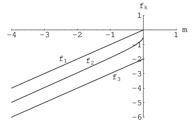
We will give our primary numerical result and two different numerical methods for showing it. But first let us give two simple mathematically rigorous lemmas that support this upcoming numerical result. Both of these results are immediate from the Rayleigh quotient formulation for $\lambda_{0}$ above. The first lemma is also shown in Proposition 4.4 of [15], with different notations.

Lemma 7.

For a nodoid of mean curvature $1$ and mass $m$, the first eigenvalue $\lambda_{0}$ of $\mathcal{L}_{0}$ satisfies $m-2\leq\lambda_{0}\leq m$.

Proof.

Using the Rayleigh quotient characterization (14), this follows directly from the fact that $-m\leq V=V(t)\leq 2-m$ for all $t$, as shown in Lemma 2. ∎

We then immediately have:

Corollary 8.

For nodoids of mean curvature $1$ and mass $m$, the first bifurcation point occurs for some $m$ between $-4$ and $-2$.

Lemma 9.

For a nodoid of mean curvature $1$ and mass $m$, the first eigenvalue $\lambda_{0}$ of $\mathcal{L}_{0}$ satisfies $\lambda_{0}\leq\frac{-1}{b-a}\int_{a}^{b}Vdt$.

Proof.

Inserting $u\equiv 1$ into the Rayleigh quotient in Equation (14), this lemma follows. ∎

Numerically checking that $\frac{-1}{b-a}\int_{a}^{b}Vdt$ is an increasing function of $m<0$ that becomes $-4$ when (and only when) $m$ is approximately $-3.036$, we have the following:

Preliminary numerical result. For nodoids of mean curvature $1$ and mass $m$, the first bifurcation point occurs for some $m\geq-3.036$.

Now, armed with the knowledge that the bifurcation point must occur for some $m$ between $-3.036$ and $-2$, we state our primary numerical result:

Primary numerical result. For a nodoid of mean curvature $1$ and mass $m$, the first eigenvalue $\lambda_{0}$ of $\mathcal{L}_{0}$ is

$$\lambda_{0}=m-1\;.$$

Hence the first bifurcation point for nodoids occurs when $m=-3$.

By the formula (8), $m=-3$ precisely when the neck radius is $r=1/2$, thus the numerical result stated in the introduction is a direct corollary of this numerical result here.

7. First method

In this and the next section we give two independent methods for numerically confirming our primary numerical result. The first method in this section is the simpler of the two.

We wish to solve

(15) $$\frac{d^{2}}{dt^{2}}u+(V+\lambda)u=0$$

for some $\lambda\in[m-2,m]$ and some function $u=u(t)\in\hat{\mathcal{F}}$. If there is only one such value for $\lambda<-1$ in the range $[m-2,m]$ (and we will see that this is the case), then this $\lambda$ will be the first eigenvalue $\lambda_{0}$. We begin with a mathematically rigorous lemma that this first numerical method is based on:

Lemma 10.

We fix any $m<0$ and consider the eigenvalue equation (15). Let $u$ be a not-identically-zero eigenfunction associated to the first eigenvalue $\lambda_{0}$. Then $u$ cannot attain zero at any value of $t$, and

$$u(\ell+t)=u(\ell-t)\;\;\;\;\text{for all}\;\;\ell\in\{a,\tfrac{3a+b}{4},\tfrac{a+b}{2},\tfrac{a+3b}{4},b\}\;.$$

In particular,

$$u^{\prime}(a)=u^{\prime}(\tfrac{3a+b}{4})=u^{\prime}(\tfrac{a+b}{2})=u^{\prime}(\tfrac{a+3b}{4})=u^{\prime}(b)=0\;.$$

Proof.

Proposition 6 tells us that the eigenspace associated to the first eigenvalue $\lambda_{0}$ must be one dimensional. If $u$ did not have all of the same symmetries as $V$ as in Lemma 2, then there would be some $\ell\in\{a,\tfrac{3a+b}{4},\tfrac{a+b}{2},\tfrac{a+3b}{4},b\}$ so that $u(\ell+t)$ and $u(\ell-t)$ are two linearly independent eigenfunctions associated to the same first eigenvalue $\lambda_{0}$. This is a contradiction, implying the lemma. ∎

$m=-1$, $\lambda=m-0.8$	$m=-1$, $\lambda=m-1.0$	$m=-1$, $\lambda=m-1.2$

$m=-2$, $\lambda=m-0.8$	$m=-2$, $\lambda=m-1.0$	$m=-2$, $\lambda=m-1.2$

$m=-3$, $\lambda=m-0.8$	$m=-3$, $\lambda=m-1.0$	$m=-3$, $\lambda=m-1.2$

Figure 3. The function $u$ computed numerically via the first method. In each case, the graph is drawn for $t\in[a,\tfrac{a+b}{2}]$ with $\tfrac{b}{3}=-a=1.3108$ (resp. $1.0$, $0.8428$) for $m=-1$ (resp. $-2$, $-3$).

Because multiplying $u$ by a real scalar does not affect Equation (15), we may assume that

$$u(\tfrac{3a+b}{4})=1\;.$$

The numerical method is then to numerically solve Equation (15) for $u$ with initial conditions

$$u(\tfrac{3a+b}{4})=1\;,\;\;\;u^{\prime}(\tfrac{3a+b}{4})=0$$

by some ODE solver (such as ”NDSolve” in Mathematica), and find the value of $\lambda$ that gives a periodic solution $u$, that is, that gives

$$u(a)=u(\tfrac{a+b}{2})=u(b)\;,\;\;\;u^{\prime}(a)=u^{\prime}(\tfrac{a+b}{2})=u^{\prime}(\tfrac{a+3b}{4})=u^{\prime}(b)=0\;,\;\;\;u(\tfrac{a+3b}{4})=1\;,\;\;\;u(t)>0\;\forall t\in[a,b]\;,$$

or equivalently, by the symmetries of $V$ in Equation (15) and by the symmetries of $u$ in Lemma 10, that simply gives

(16) $$u^{\prime}(a)=u^{\prime}(\tfrac{a+b}{2})=0\;.$$

Numerically finding this value of $\lambda$ for various values of $m<0$, one finds that it is always $m-1$, verifying the primary numerical result.

Figure 3 demonstrates how this occurs, for the cases $m=-1$, $-2$ and $-3$. In each case, the ODE solver produces a solution that satisfies Equation (16) precisely when $\lambda=m-1$. When $\lambda\in(m-1,m]$ (for example, $\lambda=m-0.8$ as in Figure 3), the values of $t$ ($\neq\tfrac{3a+b}{4}$) closest to $\tfrac{3a+b}{4}$ where $u^{\prime}(t)=0$ satisfy $|t-\tfrac{3a+b}{4}|<\tfrac{b-a}{4}$. When $\lambda\in[m-2,m-1)$ (for example, $\lambda=m-1.2$ as in Figure 3), the values of $t$ ($\neq\tfrac{3a+b}{4}$) closest to $\tfrac{3a+b}{4}$ where $u^{\prime}(t)=0$ satisfy $|t-\tfrac{3a+b}{4}|>\tfrac{b-a}{4}$. We need precisely $u^{\prime}(\tfrac{a+b}{2})=u^{\prime}(a)=0$, and this occurs exactly when $\lambda=m-1$. This has been checked for numerous other values of $m<0$ as well.

8. Second method

The second method we present here is more complicated than the first one, but we wish to consider it for the following two reasons: 1) it does not use an ODE solver and the algorithm is independent of the first method above, thus it gives a second fully-independent confirmation of the numerical result; 2) it is a stronger method in that it also gives estimates for other eigenvalues of $\mathcal{L}_{0}$, not just the first one.

As we saw in Proposition 4 and the remark just after Proposition 6, in addition to $\lambda_{0}$, $-1$ and $0$ are both also eigenvalues of $\mathcal{L}_{0}$ for all $m<0$, and $-1$ and $0$ are actually the second and third eigenvalues of $\mathcal{L}_{0}$. The fact that this second method precisely estimates the second and third eigenvalues $-1$ and $0$ gives us confidence that the method is accurately estimating $\lambda_{0}$ as well.

We choose a basis $\{\mathcal{B}_{j}=\mathcal{B}_{j}(t)\}_{j=1}^{\infty}$ for $\hat{\mathcal{F}}$ as

$$\mathcal{B}_{1}=\frac{1}{\sqrt{b-a}}\;,$$

$$\mathcal{B}_{j}=\sqrt{\frac{2}{b-a}}\cdot\cos\left(\frac{\pi j(t-a)}{b-a}\right)\;\;\;\text{ for even }\;j\in 2\mbox{$Z$}^{+}\;,$$

$$\mathcal{B}_{j}=\sqrt{\frac{2}{b-a}}\cdot\sin\left(\frac{\pi(j-1)(t-a)}{b-a}\right)\;\;\;\text{ for odd }\;j\in 2\mbox{$Z$}^{+}+1\;.$$

This is an orthonormal basis for $\hat{\mathcal{F}}$ with respect to the Euclidean $L^{2}$ norm on the interval $[a,b]$. Any $u\in\hat{\mathcal{F}}$ can be expanded as

$$u=\sum_{j=1}^{\infty}a_{j}\mathcal{B}_{j}$$

for constants $a_{j}\in\mbox{$R$}$. The Rayleigh quotient characterization (14) then gives

$$\lambda_{0}=\min_{\sum_{j\geq 1}a_{j}^{2}>0}\frac{\sum_{j,k\geq 1}a_{j}a_{k}\alpha_{jk}}{\sum_{j,k\geq 1}a_{j}a_{k}}\;,$$

where

$$\alpha_{jk}=\int_{a}^{b}-\mathcal{B}_{j}\tfrac{d^{2}}{dt^{2}}\mathcal{B}_{k}dt-\int_{a}^{b}V\mathcal{B}_{j}\mathcal{B}_{k}dt\;.$$

The integrals $\int_{a}^{b}-\mathcal{B}_{j}\tfrac{d^{2}}{dt^{2}}\mathcal{B}_{k}dt$ can be explicitly computed as

$$\int_{a}^{b}-\mathcal{B}_{j}\tfrac{d^{2}}{dt^{2}}\mathcal{B}_{k}dt=\delta_{jk}\left[\frac{j}{2}\right]^{2}\frac{4\pi^{2}}{(b-a)^{2}}\;,$$

where $\delta_{jk}$ is the Kronecker-delta function and $\left[\tfrac{j}{2}\right]$ is the greatest integer less than or equal to $\tfrac{j}{2}$.

Many integrals $\int_{a}^{b}V\mathcal{B}_{j}\mathcal{B}_{k}dt$ must be computed numerically (by a numerical integrator, such as ”NIntegrate” in Mathematica), but for each $n\in\mbox{$Z$}^{+}$ ($n\geq 3$) more than half of the entries of the $n\times n$ matrix $(\int_{a}^{b}V\mathcal{B}_{j}\mathcal{B}_{k}dt)_{j,k=1}^{n}$ can be determined to be zero simply by using the symmetry properties of the functions $V$ and $\mathcal{B}_{j}$. For example, $V(a+t)=V(a-t)$ and $\mathcal{B}_{2}(a+t)=\mathcal{B}_{2}(a-t)$, but $\mathcal{B}_{3}(a+t)=-\mathcal{B}_{3}(a-t)$, and so $\int_{a}^{b}V\mathcal{B}_{2}\mathcal{B}_{3}dt$ must be zero.

Let us list the eigenvalues of $\mathcal{L}_{0}$ in increasing order as

$$\lambda_{0}<\lambda_{1}=-1<\lambda_{2}=0<\lambda_{3}\leq\lambda_{4}\leq...\to+\infty\;.$$

Each eigenvalue appears in this list the same number of times as the dimension of its eigenspace. As noted in Proposition 5, $\lim_{j\to\infty}\lambda_{j}=+\infty$.

Remark.

In fact, all eigenvalues have multiplicity at most $2$. No eigenspace can contain three independent eigenfunctions, as $\mathcal{L}_{0}$ is a second-order linear ODE.

For each $n\in\mbox{$Z$}^{+}$, the $n\times n$ matrix $(\alpha_{jk})_{j,k=1}^{n}$ is symmetric, so it also has real eigenvalues, which we list in increasing order as

$$\lambda_{0}^{(n)}\leq\lambda_{1}^{(n)}\leq\lambda_{2}^{(n)}\leq...\leq\lambda_{n-1}^{(n)}\;.$$

Rayleigh quotient characterizations for $\lambda_{j}$ and $\lambda_{j}^{(n)}$ prove that

(17) $$\lambda_{j}^{(j+1)}\geq\lambda_{j}^{(j+2)}\geq\lambda_{j}^{(j+3)}\geq...\geq\lambda_{j}\;.$$

Thus the limit $\lim_{n\to\infty}\lambda_{j}^{(n)}$ exists and is greater than or equal to $\lambda_{j}$. Using that $\{\mathcal{B}_{j}=\mathcal{B}_{j}(t)\}_{j=1}^{\infty}$ is an orthonormal basis of $\hat{\mathcal{F}}$, and so has dense span in $\hat{\mathcal{F}}$ with respect to the $L^{2}$ norm, further arguments with Rayleigh quotient characterizations give that in fact the limit is exactly equal to $\lambda_{j}$:

Theorem 11.

([22]) $\lim_{n\to\infty}\lambda_{j}^{(n)}=\lambda_{j}$.

Theorem 11 is proven in [22]. The essential facts behind its proof are well established and can be found in many sources ([3], [5], [26] for example), but we reference [22] because the result is given there in a situation exactly analogous to the one here. This result is a simple variant of the basic theory in finite element methods (see the introductory chapters of [25] and [4], for example), and it is essentially only a variant of the Ritz-Galerkin method (see [18], for example).

This theorem now provides us with our second numerical method for estimating $\lambda_{0}$ (and any other eigenvalue of $\mathcal{L}_{0}$) by simply finding the smallest eigenvalue (and other eigenvalues) of the matrix $(\alpha_{jk})_{j,k=1}^{n}$ for sufficiently large $n$. By the inequalities (17), it is clear that the estimates will be from above. Numerical results are shown in Table 1, and they again confirm the primary numerical result in this paper.

Remark.

Symmetries of the first eigenfunction can allow us to remove some $\mathcal{B}_{j}$, if we are only looking for the first eigenvalue $\lambda_{0}$. If $u$ is the eigenfunction for the first eigenvalue, then the symmetries of $u$ in Lemma 10 imply that $u=\sum_{j\geq 1}a_{j}\mathcal{B}_{j}$ with $a_{j}=0$ when $j\geq 2$ is not an integer multiple of four. Then we can more quickly estimate $\lambda_{0}$ by using subspaces of $\hat{\mathcal{F}}$ spanned by only $\mathcal{B}_{1}$ and $\mathcal{B}_{4k}$ for $k\in\mbox{$Z$}^{+}$. However, this shortcut will not work for estimating the other eigenvalues of $\mathcal{L}_{0}$.

		Lemma	Lemma	First	Second	Second	Second	Second	Second
	$\tfrac{b}{3}=$	7’s lower	9’s upper	method’s	method’s	meth.’s	meth.’s	meth.’s	meth.’s
$m$	$=-a$	bound	bound	estimate	estimate	est.	est.	est. for	est. for
		for $\lambda_{0}$	for $\lambda_{0}$	for $\lambda_{0}$	for $\lambda_{0}$	for $\lambda_{1}$	for $\lambda_{2}$	$\lambda_{3}$, $\lambda_{4}$	$\lambda_{5}$, $\lambda_{6}$
$-1/4$	$2.0137$	$-2.25$	$-1.0522$	$-1.25$	$-1.245$	$-0.992$	$0.00543$	$1.44$	$4.45$
$-1/2$	$1.656$	$-2.5$	$-1.3643$	$-1.5$	$-1.4994$	$-0.9987$	$0.00102$	$2.279$	$6.75$
$-1$	$1.3108$	$-3$	$-1.9137$	$-2$	$-1.999$	$-0.9993$	$0.00062$	$3.86$	$11.021$
$-2$	$1.0$	$-4$	$-2.9483$	$-3$	$-2.999$	$-0.9932$	$0.00615$	$6.94$	$19.26$
$-3$	$0.8428$	$-5$	$-3.964$	$-4$	$-3.999$	$-0.999$	$0.00069$	$9.943$	$27.3$
$-10$	$0.4849$	$-12$	$-10.988$	$-11$	$-10.999$	$-0.9974$	$0.00256$	$30.99$	$83.46$
$-20$	$0.34683$	$-22$	$-20.994$	$-12$	$-20.999$	$-0.983$	$0.0168$	$61.056$	$163.61$

Table 1. Estimates for $\lambda_{0}$ and other eigenvalues of $\mathcal{L}_{0}$ (computed using the values $H=1$ and $n=13$).

Wayne Rossman:  Department of Mathematics, Faculty of Science, Kobe University, Rokko, Kobe 657-8501, Japan.   E-mail: wayne@math.kobe-u.ac.jp   web page: www.math.kobe-u.ac.jp

References

- [1] L. Barbosa and M. do Carmo, Stability of hypersurfaces with constant mean curvature, Math. Z. 185, 339-353 (1984).
- [2] L. Barbosa, J.M. Gomes and A. M. Silveira, Foliation of -dimensional space form by surfaces with constant mean curvature, Bol. Soc. Bras. Mat. 18, 1-12 (1987).
- [3] P. Bérard, Spectral Geometry: Direct and Inverse Problems, Lecture Notes in Math. 1207, Springer-Verlag, 1986.
- [4] S. C. Brenner and L. R. Scott, The Mathematical Theory of Finite Element Methods, Texts in Applied Math. 15, Springer-Verlag, 1994.
- [5] I. Chavel, Eigenvalues in Riemannian Geometry, Academic Press Inc., 1976.
- [6] S.-Y. Cheng, Eigenfunctions and nodal sets, Comment. Math. Helv. 51, 43-55 (1976).
- [7] J. Choe, Index, vision number, and stability of complete minimal surfaces, Arch. Rat. Mech. Anal. 109, 195-212 (1990).
- [8] J. Dorfmeister, F. Pedit and H. Wu, Weierstrass type representation of harmonic maps into symmetric spaces, Comm. Anal. Geom. 6, 633-668 (1998).
- [9] J. Dorfmeister and H. Wu, Construction of constant mean curvature trinoids from holomorphic potentials, preprint (2000).
- [10] N. Kapouleas, Complete constant mean curvature surfaces in Euclidean three space, Annals of Math. 131, 239-330 (1990).
- [11] N. Kapouleas, Compact constant mean curvature surfaces in Euclidean three space, J. Diff. Geom. 33, 683-715 (1991).
- [12] M. Kilian, S-P. Kobayashi, W. Rossman and N. Schmitt, Constant mean curvature surfaces with Delaunay ends in 3-dimensional space forms, preprint, math.DG/0403366v2 (2004).
- [13] N. Korevaar, R. Kusner and B. Solomon, The structure of complete embedded surfaces with constant mean curvature, J. Differential Geom. 30, 465-503 (1989).
- [14] R. Kusner, R. Mazzeo and D. Pollack, The moduli space of complete embedded constant mean curvature surfaces, Geom. Funct. Anal. 6, 120–137 (1996).
- [15] R. Mazzeo and F. Pacard, Bifurcating nodoids, Topology and geometry, Contemp. Math., vol. 314, Amer. Math. Soc., 2002, pp. 169–186.
- [16] R. Mazzeo and F. Pacard, Constant mean curvature surfaces with Delaunay ends, Comm. Anal. Geom. 9, No. 1, 169–237 (2001).
- [17] R. Mazzeo, F. Pacard and D. Pollack, The conformal theory of Alexandrov embedded constant mean curvature surfaces in , math.DG/0110099 (2001), to appear in the proceedings of the 2001 MSRI/Clay workshop on the global theory of minimal surfaces.
- [18] S. G. Mikhlin, Variational Methods in Mathematical Physics, Pergamon Press, 1964.
- [19] F. Pacard, personal communication.
- [20] K. Polthier, JavaView software, version 2.21, http://www-sfb288.math.tu-berlin.de/vgp/javaview/, April 2003.
- [21] J. Ratzkin, An end-to-end gluing construction for surfaces of constant mean curvature, doctoral thesis, University of Washington (2001).
- [22] W. Rossman, The Morse index of Wente tori, Geom. Dedicata 86, 129-151 (2001).
- [23] N. Schmitt, Constant mean curvature trinoids, preprint, math.DG/0403036, 2004.
- [24] N. Schmitt, cmclab software, http://www.gang.umass.edu/software and http://tmugs.math.metro-u.ac.jp/
- [25] G. Strang and G. J. Fix, An Analysis of the Finite Element Method, Prentice-Hall, 1973.
- [26] H. Urakawa, Geometry of Laplace-Beltrami operator on a complete Riemannian manifold, Advanced Studies in Pure Mathematics, Progress in Differential Geometry 22, 347-406 (1993).