On the Nondegeneracy of Constant Mean Curvature Surfaces

Abstract

We prove that many complete, noncompact, constant mean curvature (CMC) surfaces $f:\Sigma\rightarrow\mathbb{R}^{3}$ are nondegenerate; that is, the Jacobi operator $\Delta_{f}+|A_{f}|^{2}$ has no $L^{2}$ kernel. In fact, if $\Sigma$ has genus zero and $f(\Sigma)$ is contained in a half-space, then generically the dimension of the $L^{2}$ kernel is at most the number of non-cylindrical ends of $f(\Sigma)$, minus three. Our main tool is a conjugation operation on Jacobi fields which linearizes the conjugate cousin construction. Consequences include partial regularity for CMC moduli space, a larger class of CMC surfaces to use in gluing constructions, and a surprising characterization of CMC surfaces via rolling spheres.

1 Introduction

Constant mean curvature surfaces in $\mathbb{R}^{3}$ are equilibria for the area functional, subject to an enclosed-volume constraint. The mean curvature is nonzero when the constraint is in effect, so we can scale and orient the surfaces to make their mean curvature $1$, a condition we abbreviate by CMC. Over the past two decades a great deal of progress has been made on understanding complete CMC surfaces and their moduli spaces, however many interesting open problems remain. One of the most important questions concerns the possibility of decaying Jacobi fields on complete CMC surfaces, that is, the Morse-theoretic degeneracy of these equilibria. The main result of this paper is to rule out such Jacobi fields on a large class of complete CMC surfaces.

For a given immersed surface $f:\Sigma\rightarrow\mathbb{R}^{3}$, its mean curvature $H_{f}$ is determined by the quasilinear elliptic equation

$$\Delta_{f}f=2H_{f}\nu_{f},$$

where $\nu=\nu_{f}$ is the (mean curvature, or inner) unit normal to $f$ and $\Delta_{f}$ is the Laplace-Beltrami operator. The surface $f(\Sigma)$ is CMC if $H_{f}\equiv 1$. The oldest examples of CMC surfaces are the sphere of radius $1$ and cylinder of radius $1/2$. Interpolating between these two examples are the Delaunay unduloids, which are rotationally symmetric and periodic. A Delaunay unduloid is determined (up to rigid motion) by its necksize $n$, which is the length of the smallest closed geodesic on the surface. A necksize of $n=\pi$ corresponds to a cylinder of radius $1/2$, and as $n\rightarrow 0$ one obtains the singular limit of a chain of mutually tangent unit spheres. The ODE determining the Delaunay surfaces still has global solutions when the necksize parameter is any negative number; in this case the resulting Delaunay nodoids are not embedded.

In the present paper we will study CMC surfaces in $\mathbb{R}^{3}$ which are Alexandrov-immersed. A proper immersion $f:\Sigma\rightarrow\mathbb{R}^{3}$ is an Alexandrov immersion if one can write $\Sigma=\partial M$, where $M$ is a three-manifold into which the mean curvature normal $\nu$ points, and $f$ extends to a proper immersion of $M$ into $\mathbb{R}^{3}$. In the finite topology CMC setting, $M$ is necessarily a handlebody with a solid cylinder attached for each end. For example, the Delaunay unduloids are Alexandrov-immersed (in fact, embedded), but the Delaunay nodoids are not.

In the remainder of this paper, all of the CMC surfaces are assumed to be complete, Alexandrov immersions of finite topology, or subsets of such surfaces.

It is a theorem of Alexandrov [A] that the only compact, connected, Alexandrov-immersed, CMC surfaces are unit spheres. Here we are primarily interested in noncompact CMC surfaces. Korevaar, Kusner and Solomon [KKS] proved that each end of such a CMC surface is exponentially asymptotic to a Delaunay unduloid, that two-ended CMC surfaces are unduloids, and that three-ended CMC surfaces have a plane of reflection symmetry. In fact, all triunduloids (three-ended, genus zero CMC surfaces) were constructed and classified by Große-Brauckmann, Kusner and Sullivan [GKS], as were all coplanar $k$–unduloids ($k$–ended, genus zero CMC surfaces whose asymptotic axes all lie in a plane [GKS2]). These authors define a classifying map assigning each coplanar $k$–unduloid an immersed polygonal disc with $k$ geodesic edges in $S^{2}$, whose edge-lengths are the asymptotic necksizes of the corresponding $k$–unduloid.

The classifying map of [GKS, GKS2] is a homeomorphism, and gives information about the topological structure of moduli space of coplanar $k$–unduloids. To obtain information about the smooth structure of moduli space, one needs to understand the linearization of the mean curvature operator, which is the Jacobi operator

$$\mathcal{L}_{f}=\Delta_{f}+|A_{f}|^{2},$$

where $|A_{f}|$ is the length of the second fundamental form of $f$. Solutions to the Jacobi equation $\mathcal{L}_{f}u=0$ are called Jacobi fields, and correspond to normal variations of the CMC surface $f(\Sigma)$ which preserve the mean curvature to first order. More precisely, if $u$ is a Jacobi field, then the one-parameter family of immersions $f(t)=f+tu\nu$ has mean curvature $H(t)=1+O(t^{2})$. Thus one can think of Jacobi fields as tangent vectors to the moduli space of constant mean curvature surfaces.

Definition 1

A surface $f:\Sigma\rightarrow\mathbb{R}^{3}$ is nondegenerate if the only solution $u\in L^{2}$ to $\mathcal{L}_{f}u=0$ is the zero function.

Near a nondegenerate CMC surface $f(\Sigma)$, a theorem of Kusner, Mazzeo and Pollack [KMP] shows that the moduli space of CMC surfaces is a real-analytic manifold with coordinates derived from the asymptotic data of [KKS] (that is, the axes, necksizes, and neckphases of the unduloid asymptotes). In general the CMC moduli space is a real-analytic variety. Indeed, on a degenerate CMC surface, there would be a nonzero $L^{2}$ Jacobi field $u$, which (by [KMP]) decays exponentially on all ends. The presence of such a Jacobi field means there exists a one-parameter family of surfaces $f(t)$ with the same asymptotic data and with mean curvature $1+O(t^{2})$, indicating a possible singularity in the CMC moduli space. Thus, proving nondegeneracy eliminates the potential for such singularities.

Our main theorem bounds the dimension of the space of $L^{2}$ Jacobi fields on a large class of CMC surfaces.

Theorem 1

Let $f:\Sigma\rightarrow\mathbb{R}^{3}$ be a coplanar $k$–unduloid. Then the space of $L^{2}$ Jacobi fields on $f(\Sigma)$ is at most $(k-2)$–dimensional. Moreover, if the span of the vertices of the classifying geodesic polygon in $S^{2}$ is $\mathbb{R}^{3}$, then the space of $L^{2}$ Jacobi fields on $f(\Sigma)$ is at most $(k-3)$–dimensional.

As a corollary, we deduce that almost all triunduloids are nondegenerate. Recall ([GKS] and our earlier discussion) that a triunduloid uniquely determines a spherical triangle whose edge-lengths are the asymptotic necksizes $n_{1},n_{2},n_{3}$. The spherical triangle inequalities imply $n_{1}+n_{2}+n_{3}\leq 2\pi$ and $n_{i}+n_{j}\geq n_{k}$. When these inequalities are strict, the vertices of the classifying triangle span $\mathbb{R}^{3}$, and so our main theorem asserts that the space of $L^{2}$ Jacobi fields is $\{0\}$.

Corollary 2

Let $f:\Sigma\rightarrow\mathbb{R}^{3}$ be a triunduloid. Then $f$ is nondegenerate if its necksizes satisfy the strict spherical triangle inequalities.

When a coplanar $k$–unduloid has cylindrical ends, Theorem 20 improves the dimension bound in Theorem 1, and shows many of these CMC surfaces are also nondegenerate (see Section 6).

The main tool we develop is a conjugate Jacobi field construction, which converts Neumann fields to Dirichlet fields. This conjugate variation field arises from linearizing the conjugate cousin construction of [GKS]. Our construction is motivated by the analogous nondegeneracy result of Cosín and Ros [CR] for coplanar minimal surfaces. However, the geometry in the present case, and thus the proof, is quite different, with interesting consequences. For example, we obtain new insight into the classifying map for triunduloids and, more generally, for coplanar $k$–unduloids (see [GKS, GKS2]). The conjugate Jacobi field construction also yields a simple, synthetic characterization of constant mean curvature in terms of rolling a sphere along the surface (see Section 4).

The paper is organized as follows. Notation and preliminary computations appear in Section 2. The conjugate Jacobi field construction is in Section 3. In Section 4 we develop the rolling sphere characterization for CMC surfaces, and the interpretation of the classifying map for coplanar $k$–unduloids. The proofs of Theorem 1 and Corollary 2 are in Section 5. Finally, we discuss some extensions and applications, as well as pose some related open questions, in Section 6.

As with any mathematical problem which has been outstanding for so long, the present paper has benefited from fruitful discussion with many people. In particular, we wish to thank John Sullivan and Karsten Große-Brauckmann for reading earlier drafts of this paper, and for their helpful suggestions.

2 Notation and conventions

On a simply connected domain of a CMC (or minimal) surface, we find it convenient to use conformal curvature coordinates. These are coordinates $(x,y)=(x_{1},x_{2})$ on a domain $\Omega\subset\mathbb{R}^{2}$, so that the mapping $f:\Omega\rightarrow\mathbb{R}^{3}$ which parameterizes the surface satisfies

$$g_{11}:=\langle f_{x},f_{x}\rangle=\rho^{2}=\langle f_{y},f_{y}\rangle=:g_{22},\qquad g_{12}:=\langle f_{x},f_{y}\rangle=0,$$

and the (inner) unit normal $\nu$ to the surface satisfies

$$h_{11}:=\langle\nu,f_{xx}\rangle=-\langle\nu_{x},f_{x}\rangle=\rho^{2}\kappa_{1},\quad h_{22}:=\langle\nu,f_{yy}\rangle=-\langle\nu_{y},f_{y}\rangle=\rho^{2}\kappa_{2},\quad h_{12}:=\langle\nu,f_{xy}\rangle=0.$$

In other words, choosing conformal curvature coordinates amounts to simultaneously diagonalizing the first and second fundamental forms, $g$ and $h$. In these coordinates, the shape operator $A=g^{-1}h$ is diagonal with the principal curvatures $\kappa_{1},\kappa_{2}$ as its entries. Equivalently, the $x$ and $y$ coordinate lines are principal curves. Notice that $H=(\kappa_{1}+\kappa_{2})/2$ is half the trace of $A$. In what follows it will be useful to define $\kappa:=\kappa_{2}-\kappa_{1}$, and to adopt the convention $\kappa_{2}>\kappa_{1}$ (away from umbilic points). It also will be convenient to decompose the shape operator as $A=B+C$, where $C=HI$ is the trace part and $B=A-HI$ is trace-free. Thus, in conformal curvature coordinates, $A$ and $B$ have matrices

$$A=\left[\begin{array}[]{cc}\kappa_{1}&0\\ 0&\kappa_{2}\end{array}\right],\qquad B=\left[\begin{array}[]{cc}(\kappa_{1}-\kappa_{2})/2&0\\ 0&(\kappa_{2}-\kappa_{1})/2\end{array}\right]=\left[\begin{array}[]{cc}-\kappa/2&0\\ 0&\kappa/2\end{array}\right].$$

The existence of conformal curvature coordinates (away from umbilics) on a CMC surface can be seen using the Hopf differential, a holomorphic quadratic differential associated with $B$ (see [Ho]). More precisely, suppose we have any conformal coordinates $(u,v)$ on the surface, and consider the complex coordinate $w=u+iv$. The Codazzi equation implies the complex-valued function

$$\phi:=(h_{11}-h_{22})/2+ih_{12}$$

is holomorphic with respect to $w$ if and only if $H$ is constant. Under conformal changes of coordinates, the holomorphic quadratic differential

$$\Phi:=\phi(w)dw^{2}$$

is invariant. This $\Phi$ is the Hopf differential of our CMC surface.

Lemma 3

If $\Omega$ is simply connected and $f:\Omega\rightarrow\mathbb{R}^{3}$ is a conformal immersion of a CMC surface without umbilics, then there exists a conformal change of coordinates so that $f$ is an immersion with conformal curvature coordinates, and so that $\kappa>0$. Moreover, in any conformal curvature coordinates, $\kappa\rho^{2}$ is a constant.

Proof: Observe that umbilic points of $f$ are precisely the zeroes of $\Phi=\phi(w)dw^{2}$. Because $\Omega$ is simply connected and $f(\Omega)$ has no umbilics, we can pick a branch of $\sqrt{\phi(w)}$. Make a conformal change of coordinates $z=z(w)=x+iy$ by integrating the one-form

$$dz:=i\sqrt{\Phi}=i\sqrt{\phi(w)}dw.$$ (1)

Then in the $z$ coordinates, $\Phi=-dz^{2}$. This means $h_{12}=0$, and so $f(w(z))$ is an immersion in conformal curvature coordinates. Also, $h_{11}-h_{22}=-2$ implies $\kappa\rho^{2}=2$, and so $\kappa>0$.

Moreover, for any conformal curvature coordinates, $h_{12}\equiv 0$, so $-2\phi=\kappa\rho^{2}$ is a real-valued holomorphic function, and hence constant. $\square$

We now proceed with some preliminary computations using conformal curvature coordinates. These are elementary, but we include them for the convenience of the reader. Using the flat Laplacian, $\Delta_{0}=\partial_{x}^{2}+\partial_{y}^{2}$, the CMC equation is

$$\rho^{2}\Delta_{f}f=\Delta_{0}f=2f_{x}\times f_{y}=2\rho^{2}\nu,$$

and the Jacobi equation reads

$$\rho^{2}\mathcal{L}_{f}u=\Delta_{0}u+\rho^{2}(\kappa_{1}^{2}+\kappa_{2}^{2})u=0.$$ (2)

Unlike the previous lemma, the next two do not require $f$ to have constant mean curvature.

Lemma 4

If $f:\Omega\rightarrow\mathbb{R}^{3}$ is an immersion in conformal curvature coordinates, with unit normal $\nu$ and conformal factor $\rho=|f_{x}|=|f_{y}|$, then we have

$$f_{xx}=\frac{\rho_{x}}{\rho}f_{x}-\frac{\rho_{y}}{\rho}f_{y}+\kappa_{1}\rho^{2}\nu,\qquad f_{yy}=-\frac{\rho_{x}}{\rho}f_{x}+\frac{\rho_{y}}{\rho}f_{y}+\kappa_{2}\rho^{2}\nu.$$

Proof: The frame $(f_{x},f_{y},\nu)$ is orthogonal, so

$$f_{xx}=\rho^{-2}\langle f_{xx},f_{x}\rangle f_{x}+\rho^{-2}\langle f_{xx},f_{y}\rangle f_{y}+\langle f_{xx},\nu\rangle\nu,\qquad f_{yy}=\rho^{-2}\langle f_{yy},f_{x}\rangle f_{x}+\rho^{-2}\langle f_{yy},f_{y}\rangle f_{y}+\langle f_{yy},\nu\rangle\nu.$$

One can then complete the proof by differentiating the equations

$$\langle f_{x},f_{x}\rangle=\rho^{2}=\langle f_{y},f_{y}\rangle,\quad\langle f_{x},f_{y}\rangle=\langle f_{x},\nu\rangle=\langle f_{y},\nu\rangle=0.$$

$\square$

Lemma 5

If $f:\Omega\rightarrow\mathbb{R}^{3}$ is an immersion in conformal curvature coordinates and $u\in C^{2}(\Omega)$, then one can write the complex structure of the surface $f(t)=f+tu\nu+O(t^{2})$ as

$$J(t)=J_{0}+tJ_{1}+O(t^{2})$$

where

$$J_{0}=\left[\begin{array}[]{cc}0&-1\\ 1&0\end{array}\right],\qquad J_{1}=\left[\begin{array}[]{cc}0&u\kappa\\ u\kappa&0\end{array}\right].$$

Thus the coordinate-free expression for $J_{1}$ is the product $2uJ_{0}B$, where $B$ is the trace-free shape operator of $f$.

Proof: In any oriented local coordinates,

$$J=\frac{1}{\sqrt{\det(g)}}\left[\begin{array}[]{cc}-g_{12}&-g_{22}\\ g_{11}&g_{12}\end{array}\right].$$

Using conformal curvature coordinates at $t=0$, we compute the metric at $t$:

$$g_{11} = \langle f_{x}(t),f_{x}(t)\rangle=\rho^{2}(1-2tu\kappa_{1})+O(t^{2})$$

$$g_{22} = \langle f_{y}(t),f_{y}(t)\rangle=\rho^{2}(1-2tu\kappa_{2})+O(t^{2})$$

$$g_{12} = \langle f_{x}(t),f_{y}(t)\rangle=O(t^{2}).$$

Thus

$$J(t) = \frac{1}{\rho^{2}\sqrt{1-2(\kappa_{1}+\kappa_{2})tu}}\left[\begin{array}[]{cc}0&-\rho^{2}(1-2tu\kappa_{2})\\ \rho^{2}(1-2tu\kappa_{1})&0\end{array}\right]+O(t^{2})$$

$$= (1+tu(\kappa_{1}+\kappa_{2}))\left[\begin{array}[]{cc}0&-1+2tu\kappa_{2}\\ 1-2tu\kappa_{1}&0\end{array}\right]+O(t^{2}),$$

which yields the desired expansion. $\square$

Lawson [L] pioneered the conjugate cousin relation between CMC surfaces and minimal surfaces in $S^{3}$. The first order conjugate cousin construction was initiated by Karcher [K] and developed in [G, GKS]. It uses the realization of $S^{3}\subset\mathbb{R}^{4}=\mathbb{H}$ as the unit quaternions, and of $\mathbb{R}^{3}=\Im\mathbb{H}$ (the imaginary quaternions) as the Lie algebra of $S^{3}$, or as the tangent space $T_{1}S^{3}$. For imaginary quaternions $p,q\in\mathbb{R}^{3}$, we can write their product as

$$pq=-\langle p,q\rangle+p\times q.$$ (5)

In particular, orthogonal imaginary quaternions anti-commute. Thus we can also write the CMC condition $H_{f}\equiv 1$ as

$$\Delta_{0}f=2f_{x}f_{y}=2\rho^{2}\nu.$$ (6)

Let $\Omega\subset\mathbb{R}^{3}$ be a simply connected domain. Conjugate cousins $f:\Omega\rightarrow\mathbb{R}^{3}$ and $\tilde{f}:\Omega\rightarrow S^{3}$ satisy the first order system of partial differential equations

$$d\tilde{f}=\tilde{f}df\circ J_{0},$$ (7)

where $J_{0}$ is the standard complex structure on $\mathbb{R}^{2}$ and the product is the quaternion product. The integrability condition for $\tilde{f}$ reduces to the CMC equation for $f$, and in this case the resulting surface $\tilde{f}(\Omega)\subset S^{3}$ is minimal. Conversely, given a minimal immersion $\tilde{f}$, one can consider $f$ as the unknown in the system (7). Then the integrability condition for $f$ is the minimality of $\tilde{f}$, and the resulting surface $f(\Omega)\subset\mathbb{R}^{3}$ is CMC. Moreover, the immersions $f$ and $\tilde{f}$ are uniquely determined up to translation in $\mathbb{R}^{3}$ and left translation in $S^{3}$, respectively. One can also see from equation (7) that $f$ and $\tilde{f}$ are isometric (see Theorem 1.1 of [GKS]).

Lemma 6

The Jacobi operators for $f$ and $\tilde{f}$ coincide, and so we can identify Jacobi fields on the two surfaces.

Proof: In general, the Jacobi operator for a two-sided (CMC or minimal) surface with normal $\nu$ in a manifold with Ricci curvature $\operatorname{Ric}$ is

$$\mathcal{L}=\Delta+|A|^{2}+\operatorname{Ric}(\nu,\nu).$$

Since the Ricci curvature of $\mathbb{R}^{3}$ or $S^{3}$ is $0$ or $2$, respectively, for $f$ and its cousin $\tilde{f}$ we have

$$\mathcal{L}_{f}=\Delta_{f}+|A_{f}|^{2},\qquad\mathcal{L}_{\tilde{f}}=\Delta_{\tilde{f}}+|A_{\tilde{f}}|^{2}+2.$$

The two surfaces are isometric, so $\Delta_{f}=\Delta_{\tilde{f}}$. Moreover, we have (see Proposition 1.2 of [GKS])

$$\tilde{\kappa}_{1}=\kappa_{1}-1,\qquad\tilde{\kappa}_{2}=\kappa_{2}-1.$$

Thus

$$|A_{\tilde{f}}|^{2}=\tilde{\kappa}_{1}^{2}+\tilde{\kappa}_{2}^{2}=(\kappa_{1}-1)^{2}+(\kappa_{2}-1)^{2}=\kappa_{1}^{2}+\kappa_{2}^{2}-2(\kappa_{1}+\kappa_{2})+2=|A_{f}|^{2}-2.$$

$\square$

3 Existence of the conjugate cousin variation field

In this section we construct a conjugate cousin variation field $\tilde{\epsilon}$ on $\tilde{f}$ from a normal variation field $u\nu$ on $f$. The idea behind this construction is to linearize the conjugate cousin equation (7).

We begin with a CMC immersion $f:\Omega\rightarrow\mathbb{R}^{3}$ of a simply connected domain and a solution $u:\Omega\rightarrow\mathbb{R}$ to the Jacobi equation (2). In general, $u\nu$ is not the initial velocity of a one-parameter family of CMC surfaces

$$f(t)=f+tu\nu+O(t^{2}).$$

Although one can always find such a family on a sufficiently small subdomain, the families will not coincide on the overlaps of these subdomains. However, when there does exist such a one-parameter family of CMC surfaces, then one can define a conjugate cousin family

$$\tilde{f}(t)=\tilde{f}+t\tilde{\epsilon}+O(t^{2})$$

by integrating equation (7). In this case, the two families are related by the system

$$d\tilde{f}(t)=\tilde{f}(t)df(t)\circ J(t),$$ (8)

where $J(t)$ is the complex structure on $f(t)$. Surprisingly, if the domain $\Omega$ is simply connected, then an initial velocity field $\tilde{\epsilon}$ can be defined globally, even though this may not be possible for the conjugate cousin family itself.

Proposition 7

Let $p$ be a point in a simply connected domain $\Omega$. Let $f$ and $\tilde{f}$ be conjugate cousins satisfying equation (7). Then for any Jacobi field $u$ on $\Omega$, and any choice of initial velocity $\tilde{\epsilon}(p)$, there exists a unique global variation field $\tilde{\epsilon}$ on $\tilde{f}(\Omega)$ which is locally associated to $u$ in the manner described above. The field $\tilde{\epsilon}$ satisfies the first order system of linear partial differential equations

$$d\tilde{\epsilon}=\tilde{f}df\circ J_{1}+\tilde{f}d(u\nu)\circ J_{0}+\tilde{\epsilon}df\circ J_{0}.$$ (9)

Remark 1

The new variation field $\tilde{\epsilon}$ need not be a normal field along $\tilde{f}$.

Proof: We first sketch an abstract proof of the proposition, before giving a purely computational one. Small patches of a CMC surface are graphical and therefore strictly stable. Thus one can always use the implicit function theorem to solve a family of Dirichlet problems for the normal variation CMC equation, with boundary data $f(t)=f+tu\nu$. This yields a one-parameter family of CMC patches $f(t)$ with $t$ in a neighborhood of $0$, and with initial velocity $u\nu$ on such a small patch. From these CMC patches, solve equation (8) for a family $\tilde{f}(t)$ of minimal surface patches in $S^{3}$, uniquely determined for each $t$ once one specifies a basepoint $\tilde{\gamma}(t)=\tilde{f}(t)(p)$. These conjugate cousin surfaces have an initial velocity field $\tilde{\epsilon}$. Note, $\tilde{\epsilon}(p)=\tilde{\gamma}^{\prime}(0)$ can be adjusted at will. Once we show that the fields $\tilde{\epsilon}$ all satisfy the first order system (9) we deduce not only local existence for the initial value problem (as just described), but also uniqueness, since equation (7) reduces to a first order system of differential equations along any curve. Global existence and uniqueness then follow because $\Omega$ is simply connected.

To derive our governing system (9) we expand the conjugate family equation (8) (using quaternionic multiplication throughout):

$$d\tilde{f}+td\tilde{\epsilon}+O(t^{2}) = d\tilde{f}(t)=\tilde{f}(t)df(t)\circ J(t)$$

$$= (\tilde{f}+t\tilde{\epsilon}+O(t^{2}))(df+td(u\nu)+O(t^{2}))\circ(J_{0}+tJ_{1}+O(t^{2}))$$

Equating the $O(1)$ terms in this expansion gives the cousin equation (7). Equating the $O(t)$ terms yields equation (9), completing our sketch of the abstract proof.

A direct and instructive proof of Proposition 7 is to show that the first order system of partial differential equations (9) satisfies the Frobenius integrability conditions, namely that the formal mixed partial derivatives are equal. Existence and uniqueness for the initial value problem then follows directly from the Frobenius theorem and the fact that $\Omega$ is simply connected. Verifying the mixed-partials condition amounts to showing that the formal computation of $d(d\tilde{\epsilon})$ yields $0$. Differentiating and expanding equation (9), we get eight terms:

$$d(d\tilde{\epsilon}) = d(\tilde{f}df\circ J_{1})+d(\tilde{f}d(u\nu)\circ J_{0})+d\tilde{\epsilon}\wedge df\circ J_{0}+\tilde{\epsilon}d(df\circ J_{0})$$ (10)

$$= \tilde{f}df\circ J_{0}\wedge df\circ J_{1}+\tilde{f}d(df\circ J_{1})+\tilde{f}df\circ J_{0}\wedge d(u\nu)\circ J_{0}+\tilde{f}d(d(u\nu)\circ J_{0})$$

$$+\tilde{f}df\circ J_{1}\wedge df\circ J_{0}+\tilde{f}d(u\nu)\circ J_{0}\wedge df\circ J_{0}+\tilde{\epsilon}df\circ J_{0}\wedge df\circ J_{0}+\tilde{\epsilon}d(df\circ J_{0}).$$

It is easiest to analyze equation (10) term by term. We use conformal curvature coordinates to compute coordinate-free identities. Since umbilic points are isolated (we are not considering subdomains of spheres), continuity implies these identities hold everywhere. All terms are multiples of the area form $da=\rho^{2}dx\wedge dy$, and two of the terms vanish:

Lemma 8

$$df\circ J_{1}\wedge df\circ J_{0}=0=df\circ J_{0}\wedge df\circ J_{1}.$$

Proof: We compute $df\circ J_{1}\wedge df\circ J_{0}$:

$$df\circ J_{1}\wedge df\circ J_{0} = (u\kappa f_{y}dx+u\kappa f_{x})\wedge(f_{y}dx-f_{x}dy)=u\kappa(-f_{y}f_{x}dx\wedge dy+f_{x}f_{y}dy\wedge dx)$$

$$= u\kappa(f_{x}f_{y}-f_{x}f_{y})dx\wedge dy=0.$$

Here $f_{x}$ and $f_{y}$ are orthogonal, so they anti-commute. We also have

$$df\circ J_{0}\wedge df\circ J_{1}=-df\circ J_{1}\wedge df\circ J_{0}=0.$$

$\square$

Using equation (6), the next lemma implies that two more terms sum to zero:

Lemma 9

$$d(df\circ J_{0})=-\Delta_{0}fdx\wedge dy=-2\rho^{2}\nu dx\wedge dy=-2\nu da,\qquad df\circ J_{0}\wedge df\circ J_{0}=2\rho^{2}\nu dx\wedge dy=2\nu da.$$

Proof: First we compute

$$d(df\circ J_{0})=d(f_{y}dx-f_{x}dy)=f_{yy}dy\wedge dx-f_{xx}dx\wedge dy=-\Delta_{0}fdx\wedge dy=-2\rho^{2}\nu dx\wedge dy.$$

Similarly,

$$df\circ J_{0}\wedge df\circ J_{0}=(f_{y}dx-f_{x}dy)\wedge(f_{y}dx-f_{x}dy)=-f_{y}f_{x}dx\wedge dy-f_{x}f_{y}dy\wedge dx=2\rho^{2}\nu dx\wedge dy.$$

$\square$

The remaining terms involve the decomposition of the shape operator $A$ into trace-free and trace parts, $B=A-C$ and $C=HI=I$, respectively. In fact, note that $A=B+C$ is an orthogonal decomposition in the space of symmetric linear maps, so that, by the Pythagorean theorem,

$$|A|^{2}=|B|^{2}+|C|^{2}.$$

Lemma 10

$$d(df\circ J_{1})=-2[df(B\nabla u)+|B|^{2}u\nu]da.$$

Proof: We compute, using Lemmas 4 and 3:

$$d(df\circ J_{1}) = d(u\kappa f_{y}dx+u\kappa f_{x}dy)$$

$$= [u_{x}\kappa f_{x}+u\kappa_{x}f_{x}+u\kappa f_{xx}]dx\wedge dy+[-u_{y}\kappa f_{y}-u\kappa_{y}f_{y}-u\kappa f_{yy}]dy\wedge dx$$

$$= [\kappa(u_{x}f_{x}-u_{y}f_{y})+u(\kappa_{x}f_{x}-\kappa_{y}f_{y})+u\kappa(f_{xx}-f_{yy})]dx\wedge dy$$

$$= [\kappa(u_{x}f_{x}-u_{y}f_{y})+u(\kappa_{x}f_{f}-\kappa_{y}f_{y})+u\kappa(2\rho^{-1}\rho_{x}f_{x}-2\rho^{-1}\rho_{y}f_{y}-\kappa\rho^{2}\nu)]dx\wedge dy$$

$$= [\kappa(u_{x}f_{x}-u_{y}f_{y})+u(\kappa_{x}f_{x}+2\kappa\rho^{-1}\rho_{x}f_{x}-\kappa_{y}f_{y}-2\kappa\rho^{-1}\rho_{y}f_{y}-\kappa^{2}\rho^{2}\nu)]dx\wedge dy$$

$$= [\kappa(u_{x}f_{x}-u_{y}f_{y})+u(2\rho^{-2}\partial_{x}(\kappa\rho^{2})f_{x}-2\rho^{-2}\partial_{y}(\kappa\rho^{2})f_{y}-\kappa^{2}\rho^{2}\nu)]dx\wedge dy$$

$$= [\kappa(u_{x}f_{x}-u_{y}f_{y})-\kappa^{2}\rho^{2}u\nu]dx\wedge dy=-2[df(B\nabla u)+|B|^{2}u\nu]da.$$

$\square$

The next term we have is:

Lemma 11

$$d(d(u\nu)\circ J_{0})=2[df(A\nabla u)+|A|^{2}u\nu]da.$$

Proof: We compute, using the Jacobi equation:

$$d(d(u\nu)\circ J_{0}) = d((u\nu)_{y}dx-(u\nu)_{x})dy)=-\Delta_{0}(u\nu)dx\wedge dy$$

$$= -[u\Delta_{0}\nu+(\Delta_{0}u)\nu+2\langle\nabla u,\nabla\nu\rangle]dx\wedge dy$$

$$= -[-u\rho^{2}|A|^{2}\nu-\rho^{2}|A|^{2}u\nu+2u_{x}\nu_{x}+2u_{y}\nu_{y}]dx\wedge dy$$

$$= (2\kappa_{1}u_{x}f_{x}+2\kappa_{2}u_{y}f_{y}+2\rho^{2}|A|^{2}u\nu)dx\wedge dy=2[df(A\nabla u)+|A|^{2}u\nu]da.$$

$\square$

The final two terms actually coincide:

Lemma 12

$$d(u\nu)\circ J_{0}\wedge df\circ J_{0}=-[df(C\nabla u)+|C|^{2}u\nu]da=df\circ J_{0}\wedge d(u\nu)\circ J_{0}.$$

Proof: Using the conformality relations $\nu f_{x}=f_{y}$ and $\nu f_{y}=-f_{x}$, we have

$$d(u\nu)\circ J_{0}\wedge df\circ J_{0} = ((u_{y}\nu+u\nu_{y})dx-(u_{x}\nu+u\nu_{x})dy)\wedge(f_{y}dx-f_{x}dy)$$

$$= ((u_{y}\nu-\kappa_{2}uf_{y})dx-(u_{x}\nu-\kappa_{1}f_{x})dy)\wedge(f_{y}dx-f_{x}dy)$$

$$= (-u_{y}\nu f_{x}+\kappa_{2}uf_{y}f_{x})dx\wedge dy+(-u_{x}\nu f_{y}+\kappa_{1}uf_{x}f_{y})dy\wedge dx$$

$$= (-u_{y}f_{y}-\kappa_{2}\rho^{2}u\nu)dx\wedge dy+(u_{x}f_{x}+\kappa_{1}\rho^{2}u\nu)dy\wedge dx$$

$$= (-u_{x}f_{x}-u_{y}f_{y}-(\kappa_{1}+\kappa_{2})\rho^{2}u\nu)dx\wedge dy$$

$$= (-u_{x}f_{x}-u_{y}f_{y}-2\rho^{2}u\nu)dx\wedge dy=-[df(C\nabla u)+|C|^{2}u\nu]da,$$

since CMC implies the trace-part $C=I$ and thus $|C|^{2}=2$. The other computation is similar. $\square$

Summing the results of the previous lemmas:

$$d(d\tilde{\epsilon})=2\tilde{f}[df((A-B-C)\nabla u)+(|A|^{2}-|B|^{2}-|C|^{2})u\nu]da=2\tilde{f}[0+0]=0.$$

This completes the proof of the proposition. $\square$

4 Homogeneous solutions, rolling spheres, and the classifying map via pole solutions

We continue to consider a simply connected CMC surface $f:\Omega\rightarrow\mathbb{R}^{3}$ and its conjugate cousin surface $\tilde{f}:\Omega\rightarrow S^{3}$. At this point, it is useful to pull the variation field $\tilde{\epsilon}$ back to $\mathbb{R}^{3}=T_{1}S^{3}$. Thus we define

$$\epsilon:=\tilde{f}^{-1}\tilde{\epsilon}.$$

By the product rule and equation (7), we have

$$d\tilde{\epsilon}=d(\tilde{f}\epsilon)=\tilde{f}(df\circ J_{0})\epsilon+\tilde{f}d\epsilon;$$

however, by equation (9),

$$d\tilde{\epsilon}=\tilde{f}df\circ J_{1}+\tilde{f}d(u\nu)\circ J_{0}+\tilde{\epsilon}df\circ J_{0}=\tilde{f}(df\circ J_{1}+d(u\nu)\circ J_{0}+\epsilon df\circ J_{0}).$$

Equating these two expressions, solving for $d\epsilon$, and applying equation (5), one obtains

$$d\epsilon=\epsilon(df\circ J_{0})-(df\circ J_{0})\epsilon+df\circ J_{1}+d(u\nu)\circ J_{0}=2\epsilon\times df\circ J_{0}+df\circ J_{1}+d(u\nu)\circ J_{0}.$$ (11)

4.1 Homogeneous solutions and rolling spheres

Equation (11) is an inhomogeneous first order differential system for $\epsilon$, where the inhomogeneity $df\circ J_{1}+d(u\nu)\circ J_{0}=(-2df\circ Bu+d(u\nu))\circ J_{0}$ depends linearly on the Jacobi field $u$. The general solution to such a system is the superposition of a particular with the general solution to the associated homogeneous system. Hence we first study the homogeneous system ($u\equiv 0$) associated to (11):

$$d\epsilon=\epsilon(df\circ J_{0})-(df\circ J_{0})\epsilon=2\epsilon\times df\circ J_{0}.$$ (12)

Notice that equation (12) implies $\epsilon$ is perpendicular to $d\epsilon$, so

$$d(|\epsilon|^{2})=2\langle d\epsilon,\epsilon\rangle=0,$$

and the solutions $\epsilon$ to the linear system (12) have globally constant length. It follows that one can use them to define a path-independent parallel transport along $f(\Omega)$, mapping $T_{f(p)}\mathbb{R}^{3}\rightarrow T_{f(q)}\mathbb{R}^{3}$ isometrically. To see this, let $\gamma$ be path from $p$ to $q$ on the simply connected domain $\Omega$. One recovers $\epsilon(f(q))$ by integrating the solution to the initial value problem for equation (12), with initial value $\epsilon_{0}=\epsilon(f(p))$. Since this parallel transport is path independent, it defines a flat connection on a principal $SO(3)$-bundle over $\Omega$.

There is an interesting physical interpretation of this flat connection. Notice that if one integrates equation (12) along any curve $\gamma$ then a solution $\epsilon$ with unit length rotates with constant angular speed $2$, with evolving axis of rotation given by the curve conormal, $df\circ J_{0}(\gamma^{\prime}(s))=\eta(s)$. Note that the way to roll a sphere along the surface, without twisting or slipping, so that total rotation is minimized, is to have the sphere rotate about an axis parallel to the contact curve conormal. (Precisely, the total rotation is the length of a path in $SO(3)$, which we minimize subject to the constraint that the rolling sphere is tangent to $f(\Omega)$ as it traverses $f(\gamma)$.) If the sphere has radius $1/2$, and the contact point moves at speed $1$, then the angular speed of rotation is $2$. If the surface $f(\Omega)$ has mean curvature $1$, and if the radius–$1/2$ sphere is on the outside of the surface relative to the inner normal $\nu$, then the rolling sphere exactly reproduces our flat connection. (One must allow the sphere to immerse through the surface as necessary, for example near points with a principal curvature less that $-2$; in fact, the sphere should really roll with axis tangent to the CMC surface, but that equivalent rolling motion would be impossible to carry out physically.) In particular, if the rolling sphere follows a (contractible) loop on the surface, it will return with its initial orientation. This even gives a surprising property on a round sphere. The physical realization of this mathematical fact would make an interesting demonstration.

Proposition 13

Let $f:\Omega\rightarrow\mathbb{R}^{3}$ be an immersion and consider the $SO(3)$-connection defined by rolling a sphere of radius $1/2$ as described above. Then $f(\Omega)$ has mean curvature $1$ if and only if this connection is flat.

Proof: Since we have just shown that the CMC condition implies the flatness, it remains to prove the reverse implication. The assumption that the rolling sphere connection is flat is exactly the hypothesis that equation (12) is integrable for $\epsilon$ on any simply connected domain $\Omega$, for any choice of initial vector $\epsilon(f(p))$. Using equation (12), integrability implies

$$0=d(d\epsilon)=2[2(\epsilon\times df\circ J_{0})\times df\circ J_{0}]+2\epsilon\times(d(df\circ J_{0})).$$

The second term is $2\epsilon\times(-\Delta_{0}f)dx\wedge dy$. Expand the first term and then use the Jacobi identity:

$$4(\epsilon\times df\circ J_{0})\times df\circ J_{0} = 4(\epsilon\times(f_{y}dx-f_{x}dy))\times(f_{y}dx-f_{x}dy)$$

$$= 4(-(\epsilon\times f_{y})\times f_{x}+(\epsilon\times f_{x})\times f_{y})dx\wedge dy=4\epsilon\times(f_{x}\times f_{y})dx\wedge dy.$$

Now combine these two terms to obtain

$$0=d(d\epsilon)=2\epsilon\times(2f_{x}\times f_{y}-\Delta_{0}f)dx\wedge dy.$$

Because $\epsilon$ can be chosen to have any value at a point, we deduce that $f$ solves equation (6). $\square$

The solutions $\epsilon$ to the homogeneous system (12) can also be expressed naturally in terms of the quaternion geometry of $S^{3}$ and the conjugate surface equation for $\tilde{f}:\Omega\rightarrow S^{3}.$ Following the ideas in the abstract sketch of the proof of Propsition 7, let

$$q(t)=1+t\alpha+O(t^{2})$$

be a smooth curve of unit quaternions, passing through $1$ at time $t=0$, with $\alpha\in T_{1}S^{3}=\mathbb{R}^{3}$, a fixed imaginary quaternion. Consider the family of left translations $q(t)\tilde{f}$ of the mapping $\tilde{f}$, and note that since the translation isometry is on the left, each of these surfaces satisfies the conjugate cousin equation, $d(q(t)\tilde{f})=(q(t)\tilde{f})df\circ J_{0}.$ Therefore, the velocity $\tilde{\epsilon}=\alpha\tilde{f}$ of the family at $t=0$ solves the homogeneous ($u\equiv 0$) version of equation (9), and

$$\epsilon:=\tilde{f}^{-1}\tilde{\epsilon}=\tilde{f}^{-1}\alpha\tilde{f}$$ (13)

solves equation (12). (One can also check by direct computation that $\epsilon=\tilde{f}^{-1}\alpha\tilde{f}$ solves equation (12).) By varying $\alpha$ one obtains in this manner the unique solution to each initial value problem for equation (12).

Continuing our interpretation of equation (13), we see that an equivalent way to understand the rolling-sphere flat connection on $f(\Omega)$ is as the pullback from $\tilde{f}(\Omega)$ to $f(\Omega)$ of a natural double covering $S^{3}\rightarrow SO(3)$, arising from quaternion conjugation: for each imaginary quaternion $\alpha\in\mathbb{R}^{3}$ and each $q\in S^{3}$, write

$$R_{q}(\alpha):=q^{-1}\alpha q.$$ (14)

We have seen that for fixed $\alpha$ the $\mathbb{R}^{3}$-valued field on $S^{3}$ defined by equation (14) pulls back to a solution of equation (12) on $f(\Omega)$. More generally, for each $q\in S^{3}$ the linear map $R_{q}$ is actually a rotation (in $SO(3)$), and the flat connection on $f(\Omega)$ is the pullback of this rotation field from $S^{3}$.

Actually the involuted conjugation map $q\rightarrow R_{q^{-1}}$ is a double covering homomorphism from $S^{3}$ to $SO(3)$. This is easy to see directly from equation (14): the identity rotation $R_{q}=I$ arises if and only if the unit $q$ commutes with all quaternions, which is equivalent to $q\in\{1,-1\}.$ The homomorphism property then implies that $R_{q_{1}}=R_{q_{2}}$ if and only if $R_{q_{1}(q_{2})^{-1}}=I$, that is, $q_{1},q_{2}$ are equal or opposite.

One can check that $q\rightarrow R_{q}$ is onto $SO(3)$ by explicitly computing the rotation given by $R_{q}$. If we write $q=\operatorname{exp}(t\beta)$, where $\beta$ is a unit imaginary quaternion, then we claim that $R_{q}$ is a rotation with axis $\beta$, and that $R_{q}$ rotates an amount $-2t$ in the positive direction about the $\beta$- axis. Quaternion algebra verifies these claims. First verify that $\beta$ is fixed by $R_{q}$:

$$R_{\operatorname{exp}(t\beta)}(\beta)=\operatorname{exp}(-t\beta)\beta\operatorname{exp}(t\beta)=\beta,$$

because the three terms in the product commute. Next consider an imaginary quaternion $\alpha$ perpendicular to $\beta$:

$$R_{\operatorname{exp}(t\beta)}(\alpha) = \operatorname{exp}(-t\beta)(\alpha\operatorname{exp}(t\beta))$$

$$= \operatorname{exp}(-t\beta)(\operatorname{exp}(-t\beta)\alpha)=\operatorname{exp}(-2t\beta)\alpha$$

$$= \cos(2t)\alpha-\sin(2t)(\beta\times\alpha).$$

Since $\{\alpha,\beta\times\alpha,\beta\}$ is positively oriented, it follows that $\alpha$ is rotated by an angle $-2t$ about the $\beta$ axis, as claimed.

We conclude from this discussion that the rotation of the rolling sphere

$$R:=R_{\tilde{f}}:\Omega\rightarrow SO(3)$$

is nothing more than the conjugate cousin $\tilde{f}$ followed by the natural covering map $S^{3}\rightarrow SO(3)$. Because $\tilde{f}$ is harmonic, so is the map $R$. (One can verify this directly using (12) to compute

$$R^{-1}\Delta_{0}R=(R^{-1}R_{x})^{2}+(R^{-1}R_{y})^{2},$$

which is the equation for a harmonic map from $\Omega\subset\mathbb{R}^{2}$ to $SO(3)$, see [U]). Furthermore, the solution $\epsilon$ to equation (13) is $R(\alpha)$.

4.2 Pole solutions to the homogeneous equation and the classifying map for coplanar $k$–unduloids

The $\epsilon$-fields which solve the homogeneous system (12) yield a new perspective on the classifying map [GKS, GKS2] for coplanar $k$–unduloids.

Let $f:\Sigma\rightarrow\mathbb{R}^{3}$ be a coplanar $k$–unduloid with asymptotic necksizes $n_{1},\dots,n_{k}$. By [KKS], $f(\Sigma)$ is Alexandrov symmetric: it has a reflection plane of symmetry, which we normalize to be the $xy$ plane; furthermore, the closures of each half of $f(\Sigma)$, $f(\Sigma^{+})=f(\Sigma)\cap\{z>0\}$ and $f(\Sigma^{-})=f(\Sigma)\cap\{z<0\}$, are graphs over a (possibly immersed) planar domain. Because $\Sigma$ has genus zero, $\Sigma^{\pm}$ are topological discs. The common boundary $\partial f(\Sigma^{\pm})$ is the union of $k$ oriented, planar, principal curves $\gamma_{1},\dots,\gamma_{k}$, where $\gamma_{j}$ connects the end $E_{j-1}$ to $E_{j}$, using the natural cyclic ordering of the ends (see [GKS2]). The configuration for a triunduloid ($k=3$) is indicated in Figure 1.

Figure 1: Triunduloid configuration from above

The evolution of solutions to equation (12) is easy to track along curves of constant conormal $\eta(s)=df\circ J_{0}(\gamma^{\prime}(s))$, since the conormal is the rotation axis. With our convention that the inner normal $\nu=\gamma^{\prime}(s)\eta(s)=\gamma^{\prime}(s)\times\eta(s)$, and our choice of curve orientation in Figure 1, we see that the rotation axis along each $\gamma_{j}$ is the vertical vector $\eta=-e_{3}$, so that the rotation appears counterclockwise from above, as indicated in the figure.

Define unit-length pole solutions $P_{1},\dots,P_{k}$ to equation (12), so that $\epsilon=P_{j}$ is the unique solution to the initial value problem on $f(\bar{\Sigma}^{+})$, with initial value $P_{j}=e_{3}$ at some point (hence all points) of $\gamma_{j}$. Then the cyclically ordered $k$-tuple of unit vector fields $(P_{1},\dots,P_{k})$ on $f(\bar{\Sigma}^{+})$ determines an oriented polygonal loop on $S^{2}$, unique up to rotation and computable at any point of $f(\bar{\Sigma}^{+})$. We can compute the pairwise $S^{2}$–distances between successive vertices by studying the asymptotic behavior along the corresponding ends. Since each end converges exponentially to a Delaunay unduloid we can find curves $c_{j}$ on end $E_{j}$ which are exponentially close to the planar necks of the limit Delaunay unduloids. Exact unduloid necks with the orientation indicated in Figure 1 have conormal pointing in the axis $a_{j}$ direction, so along the curves $c_{j}$ every solution $\epsilon$ to equation (12) satisfies

$$d\epsilon(c_{j}^{\prime})=2\epsilon\times df(J_{0}(c_{j}^{\prime}))\simeq 2\epsilon\times a_{j}.$$

This implies that (up to exponentially decaying terms, which are negligible) each unit $\epsilon$ rotates with angular speed $2$ about the $a_{j}$ axis as it traverses $c_{j}$. The total length of $c_{j}$ is $n_{j}/2$, so the total rotation angle along $c_{j}$ is $n_{j}$. Choose positively oriented frames $\{a_{j},b_{j},e_{3}\}$ for each end $E_{j}$, as indicated in Figure 1. Then as we traverse $c_{j}$ the pole solution $P_{j}$ rotates in a great circle of $S^{2}$, clockwise in the plane spanned by $b_{j}$ and $e_{3}$, and we deduce that the distance from $P_{j}$ to $P_{j+1}$ is $n_{j}$. Thus the edge lengths of the polygonal loop are exactly the necksizes $n_{1},\dots,n_{k}$ of $f(\Sigma)$. This loop is the boundary of the polygonal disc used in [GKS2] to classify coplanar $k$–unduloids.

Even in the Delaunay case ($k=2$) the $\epsilon$-fields contain useful information.

Proposition 14

Let $f(\Sigma)$ be a CMC Delaunay unduloid.

• If $f(\Sigma)$ is not a cylinder then its profile curve has period $\pi$ when parameterized by arclength (see also [GKS]).

• If $f(\Sigma^{+})$ is non-cylindrical then the only solution to equation (12) which satisfies $\langle\epsilon,\nu\rangle=0$ along both $\gamma_{1},\gamma_{2}$ is the zero solution. If $f(\Sigma^{+})$ is cylindrical, then the pole solutions $P_{1},P_{2}$ are opposites, and are tangential to $f(\Sigma^{+})$, that is $\langle P_{j},\nu\rangle\equiv 0$. Each solution $\epsilon$ of equation (12) satisfying $\langle\epsilon,\nu\rangle=0$ along both $\gamma_{1},\gamma_{2}$ is a multiple of $P_{1}=-P_{2}$.

Proof: Starting at the initial point of $c_{1}$, follow the pole solutions around the contour in Figure 2, which depicts one period of an unduloid. We see that the pole $P_{1}$ must return to the vertical position after traversing the second neck $c_{2}$. This is only possible if $P_{1}$ has rotated through a total angle of $2\pi k$ for some positive integer $k$ as it travels from $c_{1}$ to $c_{2}$ along $\gamma_{2}$. However, $P_{1}$ rotates with speed $2$ along $\gamma_{2}$, so the length of the $\gamma_{2}$–arc must be $k\pi$. In the zero necksize limit, this arc is half a great circle on a unit sphere, so it has length $\pi$. Thus, by the continuity of the family of Delaunay unduloids, the period of each unduloid is $\pi$.

Figure 2: Delaunay configuration from above

For the second part of this proposition, suppose $\epsilon\neq 0$ solves equation (12) and $\langle\epsilon,\nu\rangle=0$ along $\gamma_{1},\gamma_{2}$. If $\epsilon$ has a nonzero horizontal component along the boundary curve $\gamma_{1}$, then as one traverses $\gamma_{1}$ this component rotates with angular speed $2$. Thus the horizontal component of $\epsilon$ will be perpendicular to the axis of the unduloid at points distributed with period $\pi/2$. At such points $\langle\epsilon,\nu\rangle\neq 0$. Therefore $\epsilon$ is vertical along $\gamma_{1}$, and $\epsilon=cP_{1}$ for some constant $c$. However, we have just seen that the pole solution $P_{1}$ has a nonzero horizontal component after traversing the neck $c_{1}$. Thus the same argument shows $c=0$.

If $f(\Sigma)$ is a cylinder then $P_{1}=-P_{2}$ and the solution $\epsilon=cP_{1}$ persists. Furthermore, $\epsilon$ remains exactly parallel to the tangent vector as it traverses the radius $1/2$ circular cross-sections of the cylinder, so it is tangent to $f(\Sigma^{+})$. $\square$

There is an interesting consequence and generalization of the fact that the period of any Delaunay unduloid is $\pi$. Consider a coplanar $k$–unduloid and let $L_{j}$ be the length of the curve $\gamma_{j}$ obtained by truncating at the (asymptotically exact) necks $c_{j-1}$ and $c_{j}$. By the previous proposition, the length mod $\pi$ of these curves has a well-defined limit as the truncations approach infinity. We call this limit $L_{j}^{\infty}$.

Proposition 15

Let $\alpha_{j}$ be the interior angle at the vertex $P_{j}$ of the spherical polygon associated to $f(\Sigma)$, and let $\beta_{j}$ be the angle between the asymptotic axes $a_{j-1}$ and $a_{j}$ (see Figure 1). Then

$$2L_{j}^{\infty}=\pi+\alpha_{j}+\beta_{j}\mbox{ mod }2\pi.$$

Remark 2

This result is equivalent to the relation found (Proposition $7$ of [GKS0]) for the twist angle of the conjugate cousin minimal surface around each of its boundary Hopf circles.

Proof: One can see from equation (12) that after traversing $\gamma_{j}$, the horizontal components of the arc from $P_{j-1}$ to $P_{j}$ have rotated through an angle $2L_{j}$. As indicated by the angle relations illustrated in Figure 3 (for $j=2$ on a triunduloid), this must be asymptotically equal (up to multiples of $2\pi$) to $\pi+\alpha_{j}+\beta_{j}$. $\square$

Figure 3: The top view of the pole solutions just before traversing the second neck

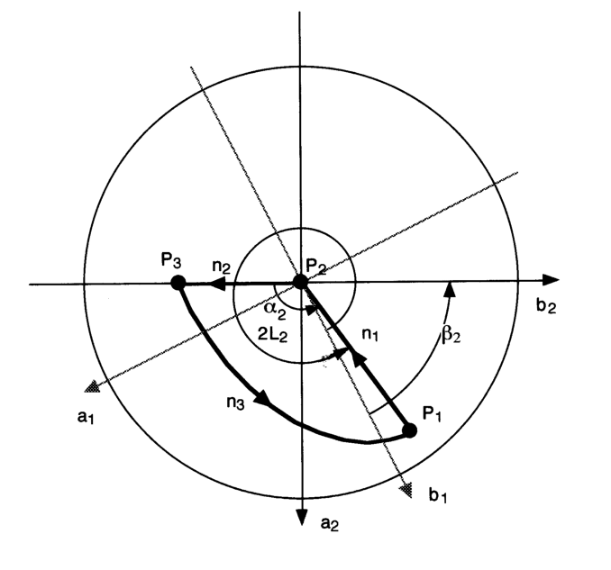
5 The proof of the main theorem

We prove Theorem 1 in this section.

The proof uses two features of the Alexandrov symmetry satisfied by a coplanar $k$–unduloid $f:\Sigma\rightarrow\mathbb{R}^{3}$. First, the reflection symmetry lets us decompose any Jacobi field $u$ into the sum of an even part $u_{+}$ and an odd part $u_{-}$. We call an even field Neumann because its restriction to $\Sigma^{+}$ satisfies

$$\mathcal{L}_{f}(u_{+})=0,\qquad\left.\frac{\partial u_{+}}{\partial\eta}\right|_{\partial\Sigma^{+}}=0,$$

where $\eta$ is the (outer) conormal to $\partial\Sigma^{+}$. Similarly, we call an odd field Dirichlet since it vanishes on $\partial\Sigma^{+}$. Second, the graphical nature of $f(\Sigma^{+})$ implies that $v:=-\langle\nu,e_{3}\rangle$ is a positive Dirichlet Jacobi field on $f(\Sigma^{+})$. Using $v$ as a comparison, we show in Section 5.1 that $0$ is the only $L^{2}$ Dirichlet Jacobi field. This analysis so far carries through for coplanar CMC surfaces of any genus.

In order to analyze the Neumann Jacobi fields in Section 5.2, we use the conjugate variation field $\tilde{\epsilon}$ constructed in Section 3. This requires $\Sigma^{+}$ to be simply connected, that is, $\Sigma$ must have genus zero.

Let $\mathcal{V}$ denote the space of $L^{2}$ Jacobi fields on $f(\Sigma)$.

5.1 Dirichlet Jacobi fields

We give two proofs of Proposition 17 below. The first proof uses the strong maximum principle to show that if $u\in L^{2}$ is a Dirichlet Jacobi field it must vanish. This proof is analogous to the standard proof that the first eigenvalue of $\Delta$ on a bounded domain $\Omega$ is simple. The second proof we present is an integral version of the same maximum principle argument, which we strengthen to deduce the result for bounded Dirichlet Jacobi fields. Both proofs compare $u$ to the vertical translation field $v=-\nu_{3}$. Notice that $v>0$ on $\Sigma^{+}$ and $v=0$ on $\partial\Sigma^{+}$.

To apply our maximum principle arguments comparing $u$ to $v$, we need to know

$$v_{\eta}:=\frac{\partial v}{\partial\eta}\leq-\delta<0$$

on $\partial\Sigma^{+}$. (We continue our convention that $\eta$ in the outer conormal, which in this case is $-e_{3}$ along $\partial\Sigma^{+}$.) One can quickly deduce this inequality for some positive $\delta$, because it is true near the ends (with $\delta=1$) and since on any compact subset of $\partial\Sigma^{+}$ the Hopf boundary point lemma gives a (noncomputable) value for $\delta$. The following lemma shows that we may take $\delta=1$ along all of $\partial\Sigma^{+}$. We include this lemma, which is a reinterpretation of height and gradient estimates carried out in [KKS, KK], for its geometric consequences.

Lemma 16

Let $f(\Sigma)$ be an Alexandrov symmetric CMC surface with finite topology. The boundary $\partial f(\Sigma^{+})$ is a union of principal curves on $f(\Sigma)$ with principal curvature $\kappa_{1}<1$. In particular, the symmetry curves do not contain umbilics, and $\kappa_{2}=\langle\nu,e_{3}\rangle_{\eta}=-v_{\eta}>1$.

Proof: Because $\partial f(\Sigma^{+})$ is the fixed point set of a reflection symmetry for $f(\Sigma)$, it is a union of principal curves.

By the CMC equation, we have

$$\Delta_{f}(z)=2\nu_{3},$$

where $z$ is the restriction of the vertical coordinate to the surface $f(\Sigma^{+})$. Also, because the components of the normal $\nu$ satisfy the Jacobi equation, we have

$$\Delta_{f}(\nu_{3})=-|A|^{2}\nu_{3}\geq-2\nu_{3},$$

Here we have used that $|A|^{2}\geq 2$ and $\nu_{3}<0$. Thus we have

$$\Delta_{f}(z+\nu_{3})=(2-|A|^{2})\nu_{3}\geq 0,$$

and so $z+\nu_{3}$ is a subharmonic function on $\Sigma^{+}$. On $\partial\Sigma^{+}$, each function vanishes, so $z+\nu_{3}=0$. By explicit computation, $z+\nu_{3}\leq 0$ on the unduloid ends of $\bar{\Sigma}^{+}$. Thus in (the interior of) $\Sigma^{+}$,

$$z+\nu_{3}<0$$

by the strong maximum principle. (Equality can only hold when $f$ parameterizes a unit hemisphere.)

By the Hopf boundary point lemma,

$$0<\frac{\partial}{\partial\eta}(z+\nu_{3})=-1+\frac{\partial\nu_{3}}{\partial\eta}=-1+\frac{\partial}{\partial\eta}\langle\nu,e_{3}\rangle.$$

We can rearrange this to obtain the curvature perpendicular to the boundary

$$\kappa_{2}=\frac{\partial}{\partial\eta}\langle\nu,e_{3}\rangle=-v_{\eta}>1,$$ (15)

and so the principal curvature along the boundary is

$$\kappa_{1}=2-\kappa_{2}<1.$$

$\square$

Proposition 17

Let $f(\Sigma)$ be an Alexandrov symmetric CMC surface (see Section 4.2) of finite genus and with a finite number of ends. Every bounded odd (Dirichlet) Jacobi field $u$ on $f(\Sigma)$ is a constant multiple of the vertical translation field $v=-\langle\nu,e_{3}\rangle=-\nu_{3}$. In particular, if $u\in\mathcal{V}$ then $u$ is an even (Neumann) Jacobi field.

First proof: After possibly replacing $u$ with $-u$, we can assume $u>0$ somewhere. Now let $\mu>0$ be a positive parameter. We assume for this first proof that $u\in\mathcal{V}$, so by [KMP] $u$ and its derivatives decay exponentially. Combining this exponential decay with inequality (15), we see that for $\mu$ sufficiently large

$$\mu v>u$$

everywhere in the interior of $\Sigma^{+}$, with equality on $\partial\Sigma^{+}$. We define

$$\mu^{*}=\inf\{\mu>0\mbox{ }|\mbox{ }\mu v(p)>u(p)\,,p\in\Sigma^{+}\}.$$

There is some finite $q$ which is a critical point of $\mu^{*}v-u$ with critical value $0$. The point $q$ lies in either the interior or the boundary of $\Sigma^{+}$. In both cases

$$u(q)=\mu^{*}v(q),\qquad\nabla u(q)=\mu^{*}\nabla v(q),$$

and $u\leq\mu^{*}v$ on $\Sigma^{+}$. In either case, the strong maximum principle (the Hopf boundary point lemma if $q\in\partial\Sigma^{+}$) implies $u\equiv\mu^{*}v$. Because $u\in L^{2}$, this implies $\mu^{*}=0$ and thus $u\equiv 0$. $\square$

Second proof: We initially assume $u\in\mathcal{V}$, rather than the more general hypothesis that $u$ is a bounded Dirichlet Jacobi field. For this proof it is technically simpler to consider the entire surface $f(\Sigma)$. Recall that both $u$ and $v$ are odd with respect to reflection through the Alexandrov plane of symmetry, and by inequality (15) $u/v$ is uniformly bounded on the complement of the symmetry curves, which is $\{v\neq 0\}$. Also, both $u$ and $v$ are real analytic functions which vanish on the symmetry curves. These facts imply that $u/v$ extends to an even, real analytic function on the entire surface $f(\Sigma)$. To verify analyticity on $\{v=0\}$, use conformal curvature coordinates in which the $x$–axis is a symmetry curve; the fact that $u$ and $v$ both vanish on the $x$–axis means we can write

$$u(x,y)=yU(x,y),\qquad v(x,y)=yV(x,y),\qquad\frac{u(x,y)}{v(x,y)}=\frac{yU(x,y)}{yV(x,y)}=\frac{U(x,y)}{V(x,y)},$$

where $U$ and $V$ are also real analytic and $V\neq 0$ near the $x$–axis by Lemma 16.

Continuing with the second proof, assume that $u/v>0$ somewhere. Since $u/v$ is nonconstant, we can pick a regular value $\delta>0$ for $u/v$ with nonempty inverse image. The domain

$$\Omega_{\delta}:=\{u/v>\delta\}$$

is bounded (because $u\in L^{2}$) and has smooth boundary in $\Sigma$. Since $(u/v)_{\eta}<0$ pointwise along $\partial\Omega_{\delta}$,

$$\int_{\partial\Omega_{\delta}}v\frac{\partial u}{\partial\eta}-u\frac{\partial v}{\partial\eta}=\int_{\partial\Omega_{\delta}}v^{2}\frac{\partial(u/v)}{\partial\eta}<0.$$ (16)

However, we also have

$$0 = \int_{\Omega_{\delta}}v\mathcal{L}_{f}u-u\mathcal{L}_{f}v=\int_{\Omega_{\delta}}v\Delta_{f}u-u\Delta_{f}v$$ (17)

$$= \int_{\partial\Omega_{\delta}}v\frac{\partial u}{\partial\eta}-u\frac{\partial v}{\partial\eta}=\int_{\partial\Omega_{\delta}}v^{2}\frac{\partial(u/v)}{\partial\eta}.$$

This last equation (17) contradicts the previous inequality (16), proving $u\equiv 0$.

We now explain how to extend this argument to prove that any bounded Dirichlet Jacobi field $u$ is a constant multiple of $v$. We assume $u/v$ is nonconstant and positive somewhere, pick a regular value $\delta>0$, and define the nonempty set $\Omega_{\delta}$ as before. In this case the inequalty (16) still holds, but we cannot immediately deduce equation (17) because $\Omega_{\delta}$ may be unbounded. We overcome this difficulty by appealing to the linear decomposition lemma of [KMP], which implies that on each end $E_{j}$, we have exponential convergence

$$u\simeq\sum_{i=1}^{3}a_{ij}\nu_{i},$$

where $\nu_{i}$ are the components of the normal vector to the asymptotic unduloid. Because $u$ is odd, we must have $u\simeq a_{j}\nu_{3}:=a_{3j}\nu_{3}$ on the end $E_{j}$, and so $u/v$ converges smoothly to a constant $-a_{j}$ on the end $E_{j}$. (A priori, these constants may differ from end to end.)

Now we truncate the domain $\Omega_{\delta}$ by intersecting $f(\Sigma)$ with a sequence of balls, defining

$$\Omega_{\delta,N}:=\{p\in\Omega_{\delta}:|f(p)|\leq N\}=\Omega_{\delta}\cap\bar{B}_{N}(0),$$

where $N=1,2,3,\dots$. Then equation (17) becomes

$$0=\int_{\Omega_{\delta,N}}u\mathcal{L}_{f}v-v\mathcal{L}_{f}u=\int_{\partial\Omega_{\delta}\cap B_{N}}uv_{\eta}-vu_{\eta}+\int_{\Omega_{\delta}\cap\partial B_{N}}uv_{\eta}-vu_{\eta}.$$ (18)

But as soon as $N$ is large enough so that $\partial\Omega_{\delta}\cap B_{N}$ has positive length, inequality (16) implies the first term is negative, and in fact it is decreasing in $N$; also, the second terms converge uniformly to zero by our previous discussion of the asymptotics. This contradiction shows $u$ is a constant multiple of $v$. $\square$

5.2 Neumann Jacobi fields

Given a Jacobi field $u$ on the coplanar $k$–unduloid $f(\Sigma)$, the conjugate field $\tilde{\epsilon}$ defined by equation (9) yields a conjugate Jacobi field $\tilde{u}:=\langle\tilde{\epsilon},\tilde{\nu}\rangle$ on the surfaces $\tilde{f}(\Sigma^{+})$ and $f(\Sigma^{+})$. By the correspondence $\tilde{\epsilon}=\tilde{f}\epsilon$ relating solutions of equations (9) and (11), we see

$$\tilde{u}=\langle\tilde{\epsilon},\tilde{\nu}\rangle=\langle\tilde{f}\epsilon,\tilde{f}\nu\rangle=\langle\epsilon,\nu\rangle.$$

Our plan is to convert even (Neumann) Jacobi fields $u\in\mathcal{V}$ into $L^{2}$ Dirichlet Jacobi fields $\tilde{u}$, use Proposition 17 to deduce $\tilde{u}\equiv 0$, and use this to show $u\equiv 0$. In order to carry out this procedure, $u$ must satisfy a finite number of linear conditions, which is why Theorem 1 only bounds the dimension of $\mathcal{V}$, rather that asserting $\mathcal{V}=\{0\}$.

Since each $u\in\mathcal{V}$ decays exponentially on all ends, the corresponding conjugate fields $\epsilon$ are asymptotic to solutions of the homogeneous equation (12). By [GKS2], $f(\Sigma)$ has at least two non-cylindrical ends, one of which we label $E_{k}$ (see Figure 1). From Proposition 14 in Section 4.2, a necessary condition for attaining zero Dirichlet data on the end $E_{k}$ is that $\epsilon$ must converge to $0$, and so we specify a unique conjugate field $\epsilon$ associated to $u$ by setting $\epsilon=0$ on this non-cylindrical end $E_{k}$. Starting at $E_{k}$, we compute how $\epsilon$ changes along the contours $\gamma_{j}$, and along the ends $E_{j}$.

By Lemma 16, the $\gamma_{j}$ are principal curves, with curvature $\kappa_{1}<1$ and constant conormal $-e_{3}$. We have seen by Proposition 17 that $u\in\mathcal{V}$ is even. Thus we have

$$d\epsilon(\gamma_{j}^{\prime}) = 2\epsilon\times df\circ J_{0}(\gamma_{j}^{\prime})+df\circ J_{1}(\gamma_{j}^{\prime})+d(u\nu)\circ J_{0}(\gamma_{j}^{\prime})$$

$$= -2\epsilon\times e_{3}+u(\kappa_{2}-\kappa_{1})f_{\eta}+u_{\eta}\nu+u\nu_{\eta}$$

$$= -2\epsilon\times e_{3}+u(\kappa_{1}-\kappa_{2}+\kappa_{2})e_{3}+u_{\eta}\nu$$

$$= -2\epsilon\times e_{3}+u\kappa_{1}e_{3}$$

along $\gamma_{j}$. The geometric interpretation of this equation is that the horizontal part of $\epsilon$ rotates about $e_{3}$, counterclockwise with speed $2$, and the vertical part of $\epsilon$ changes at a rate of $u\kappa_{1}$. Now set

$$h_{j}(u):=\int_{\gamma_{j}}d(\langle\epsilon,e_{3}\rangle)=\int_{\gamma_{j}}u\kappa_{1}ds,$$ (19)

where $s$ is the arc-length parameter along $\gamma_{j}$. These heights $h_{j}(u)$ measure the change in the vertical components of $\epsilon$ as one traverses $\gamma_{j}$. They play a key role in our analysis.

The integration defining the heights $h_{j}(u)$ associates a real number to each symmetry curve $\gamma_{j}$. We encode this by defining the linear transformation $T:\mathcal{V}\rightarrow\mathbb{R}^{k}$ by

$$T(u)=(h_{1}(u),\dots,h_{k}(u)).$$ (20)

Proposition 18

Let $f(\Sigma)$ be a coplanar $k$–unduloid, and let $\mathcal{V}$ be the space of $L^{2}$ Jacobi fields on $f(\Sigma)$. Then the linear transformation $T:\mathcal{V}\rightarrow\mathbb{R}^{k}$ defined by expression (20) is injective. In particular, the dimension of $\mathcal{V}$ is at most $k$.

Proof: We prove this proposition in two steps. First, show that $T(u)=0$ implies the conjugate Jacobi field $\tilde{u}$, which is uniquely defined by our choice that $\epsilon=0$ on the non-cylindrical end $E_{k}$, must be identically zero. The second step is to show that whenever $\tilde{u}\equiv 0$ then $u\equiv 0$.

As we traverse $\gamma_{1}$ from the end $E_{k}$ to the end $E_{1}$ only the vertical part of $\epsilon$ changes, and the total change in this component is $h_{1}(u)=0$. Thus $\epsilon(p)$ converges exponentially to $0$ on $\gamma_{1}$ as $p$ approaches infinity on the end $E_{1}$. Since $\epsilon$ also converges to a homogeneous solution on $E_{1}$, we see that $\epsilon$ converges to $0$ on the entire end $E_{1}$. Repeat this argument successively, traversing $\gamma_{j}$ from $E_{j-1}$ to $E_{j}$, using the hypothesis that each $h_{j}(u)=0$. We deduce that $\epsilon$ converges to $0$ exponentially along each end and that it remains vertical along each $\gamma_{j}$. Thus $\tilde{u}=\langle\epsilon,\nu\rangle$ decays exponentially to zero along each end and is a Dirichlet field, because $\epsilon$ is vertical and $\nu$ is horizontal along each $\gamma_{j}$. Therefore, after extending $\tilde{u}$ to all of $f(\Sigma)$ by odd reflection, Proposition 17 implies $\tilde{u}\equiv 0$.

Proceeding to the second step, we assume $\tilde{u}=\langle\tilde{\epsilon},\tilde{\nu}\rangle\equiv 0$, that is, the vector field $\tilde{\epsilon}$ is tangent to $\tilde{f}(\Sigma^{+})$. We pull $\tilde{\epsilon}$ back to $\Sigma^{+}$ and denote its flow by $X_{\tilde{\epsilon}}(t)$. For small values of $t$, this is a diffeomorphism $X_{\tilde{\epsilon}}(t):\Sigma^{+}\rightarrow\Sigma^{+}$, because $\epsilon$ is parallel to the conormal, and so $\tilde{\epsilon}$ is tangent along $\partial\tilde{f}(\Sigma^{+})$. Now define the one-parameter family of immersions

$$\tilde{f}(t)=\tilde{f}\circ X_{\tilde{\epsilon}}(t):\Sigma^{+}\rightarrow S^{3}.$$

This provides a family of reparameterizations of the minimal surface $\tilde{f}(\Sigma^{+})\subset S^{3}$.

We produce a family of CMC surfaces $f(t)$ in $\mathbb{R}^{3}$ by taking the conjugate cousin of this family of reparameterization of $\tilde{f}(\Sigma^{+})$. Rearrange the conjugate family equation (8) to read

$$df(t)=-\tilde{f}(t)^{-1}d\tilde{f}(t)\circ J(t).$$ (21)

Using the inhomogeneous equation (9) for $\epsilon$ and $\tilde{f}(t)=\tilde{f}+t\tilde{\epsilon}+O(t^{2})=\tilde{f}(1+t\epsilon+O(t^{2}))$, expand equation (21) in powers of $t$. One recovers $d(u\nu)$ as the $O(t)$ term in the expansion of $df(t)$:

$$df(t) = -(\tilde{f}(1+t\epsilon))^{-1}[(d\tilde{f})(1+t\epsilon)+t\tilde{f}d\epsilon]\circ(J_{0}+tJ_{1})+O(t^{2})$$

$$= -(1-t\epsilon)\tilde{f}^{-1}[d\tilde{f}\circ J_{0}+t((d\tilde{f}\circ J_{0})\epsilon+d\tilde{f}\circ J_{1}+\tilde{f}d\epsilon\circ J_{0})]+O(t^{2})$$

$$= -\tilde{f}^{-1}d\tilde{f}\circ J_{0}+t[\epsilon\tilde{f}^{-1}d\tilde{f}\circ J_{0}-\tilde{f}^{-1}(d\tilde{f}\circ J_{0})\epsilon-\tilde{f}^{-1}d\tilde{f}\circ J_{1}-d\epsilon\circ J_{0}]+O(t^{2})$$

$$= df+t[-\epsilon df+df\epsilon-df\circ J_{0}\circ J_{1}-(-\epsilon df+df\epsilon-d(u\nu)+df\circ J_{1}\circ J_{0})]+O(t^{2})$$

$$= df+td(u\nu)+O(t^{2}).$$

We used the facts that $J_{0}^{2}=-I$ and $J_{0}\circ J_{1}=-J_{1}\circ J_{0}$ in the last steps.

Integrate the one-form $df(t)=df+td(u\nu)+O(t^{2})$ to recover the immersion $f(t)$. In this integration we are free to choose the value of $f(t)$ at a basepoint $p\in\Sigma^{+}$, and choose $f(t)(p)=f(p)+tu\nu(p)$. Then for any compact set $K\subset\Sigma^{+}$ and $q\in K$, we have

$$f(t)(q) = f(p)+tu\nu(p)+\int_{p}^{q}df(t)$$

$$= f(p)+tu\nu(p)+\int_{p}^{q}d(f+tu\nu)+O(t^{2}))=f(q)+tu\nu(q)+O(t^{2}).$$

However, this one-parameter family $f(t)$ is a conjugate cousin family for the fixed surface $\tilde{f}(\Sigma^{+})$, so by Theorem 1.1 of [GKS], the surfaces $f(t)$ can only vary by a family of translations. Taking the derivative at $t=0$, this implies $u$ is the normal part of an $\mathbb{R}^{3}$ translation, which implies $u\not\in L^{2}$. Thus $\tilde{u}\equiv 0$ implies $u\equiv 0$, completing the proof that $T$ is injective. $\square$

Proposition 19

Suppose $f(\Sigma)$ is a coplanar $k$–unduloid. Let $u\in\mathcal{V}$, and let $P_{1},\dots,P_{k}$ be the pole solutions to the homogeneous equation (12) associated to the symmetry curves $\gamma_{1},\dots,\gamma_{k}$. Then for the constants $h_{j}:=h_{j}(u)$, we have the linear relation

$$\sum_{j=1}^{k}h_{j}P_{j}\equiv 0$$ (22)

on $f(\Sigma^{+})$. Thus, if the vertices of the classifying polygon for $f(\Sigma)$ span an $l$-dimensional subspace of $\mathbb{R}^{3}$, then $\mathcal{V}$ is at most $(k-l)$–dimensional.

Proof: Let $\epsilon$ be the conjugate variation field which solves equation (11) for the given $u\in\mathcal{V}$, with $\epsilon=0$ on the end $E_{k}$. Traversing $\gamma_{1}$ from $E_{k}$ to $E_{1}$, as in the previous proposition, we conclude that $\epsilon$ converges exponentially to the homogeneous solution $h_{1}P_{1}$ on the end $E_{1}$. Thus $\epsilon_{1}=\epsilon-h_{1}P_{1}$ solves equation (11) with inital value $0$ on $E_{1}$, and evolves along $\gamma_{2}$ with a vertical change of $h_{2}$. Thus $\epsilon_{1}$ converges to the homogeneous solution $h_{2}P_{2}$ along the end $E_{2}$, so $\epsilon$ converges to $h_{1}P_{1}+h_{2}P_{2}$ along this end. Continuing this reasoning and traversing the remaining $\gamma_{j}$ in order, one returns to the end $E_{k}$, with $\epsilon$ converging to the homogeneous solution $h_{1}P_{1}+\cdots+h_{k}P_{k}$. Since $\epsilon$ is well-defined, this sum must be the initial asymptotic homogeneous solution $0$. This shows the linear dependence (22).

Evaluating the pole solutions at a point $q\in\Sigma^{+}$ yields vertices for a representative classifying polygon for $f(\Sigma)$. The linear relation (22) implies that $(h_{1},\dots,h_{k})$ solves a homogeneous system of rank $l=\dim\operatorname{span}\{P_{1}(q),\dots,P_{k}(q)\}\leq 3$. Since the solution space of this system is $(k-l)$–dimensional, and $T$ is injective, we conclude that $\dim\mathcal{V}\leq k-l$. $\square$

Using the fact that the vertices of the classifying polygon of a coplanar $k$–unduloid span a two- or three-dimensional subspace of $\mathbb{R}^{3}$ [GKS2], this completes the proof of Theorem 1, and, as explained in the introduction, Corollary 2.

6 Extensions, applications and open questions

One can sharpen the proofs of Theorem 1 and Corollary 2 to show that triunduloids with a cylindrical end are also nondegenerate. The theorem below includes these triunduloids as a special case, and applies to a more general class of $k$–unduloids. By Theorem $1.5$ of [GKS2], a coplanar $k$–unduloid has at least two non-cylindrical ends.

Theorem 20

Let $f(\Sigma)$ be a coplanar $k$–unduloid. If $f(\Sigma)$ has $d$ non-cylindrical ends and the vertices of the classifying polygon span an $l$–dimensional subspace of $\mathbb{R}^{3}$, then the space $\mathcal{V}$ of $L^{2}$ Jacobi fields has dimension at most $d-l$. In particular, if $f(\Sigma)$ has exactly two non-cylindrical ends, or three non-cylindrical ends and classifying polygon with vertices spanning $\mathbb{R}^{3}$, then it is nondegenerate.

Proof: By Proposition 17, any $u\in\mathcal{V}$ is even, so we proceed as in Section 5.2. The key idea in the proof is the observation (see Proposition 14) that if $E_{j}$ is a cylindrical end, then the pole solutions $P_{j}$ and $P_{j+1}$ are opposites, and are asymptotically tangent along $E_{j}$. In other words, given $u\in\mathcal{V}$ and a corresponding conjugate variation field $\epsilon$, if $\epsilon$ is vertical along $\gamma_{j}$ then it is asymptotically tangent on $E_{j}$ and continues to be vertical on $\gamma_{j+1}$. Therefore, the conjugate Jacobi field $\tilde{u}=\langle\epsilon,\nu\rangle$ vanishes on $\gamma_{j}\cup\gamma_{j+1}$ and decays along $E_{j}$. More generally, if $(E_{r},\dots,E_{s-1})$ is a string of adjacent cylindrical ends and $\epsilon$ is vertical on $\gamma_{r}$, then it is vertical on all the symmetry curves $\gamma_{r}\cup\dots\cup\gamma_{s}$, implying $\tilde{u}$ vanishes on these symmetry curves and decays on the ends $E_{r},\dots,E_{s-1}$.

We now develop the combinatorial tools needed to complete the proof. The distribution of non-cylindrical ends on $f(\Sigma)$ leads to a partitioning of the cyclically ordered set of symmetry curves $(\gamma_{1},\dots,\gamma_{k})$ and their corresponding pole solutions $(P_{1},\dots,P_{k})$ into substrings of two types. A string $C:=(\gamma_{r},\gamma_{r+1},\dots,\gamma_{s})$ is cylindrical if the ends $E_{r},E_{r+1},\dots,E_{s-1}$ are cylindrical while $E_{r-1}$ and $E_{s}$ are not. In other words, $\gamma_{r}\cup\dots\cup\gamma_{s}$ connects the non-cylindrical end $E_{r-1}$ to the next non-cylindrical end $E_{s}$, through adjacent cylindrical ends. A singleton string $D:=(\gamma_{j})$ is non-cylindrical if neither $E_{j}$ nor $E_{j-1}$ are cylindrical. That is, $\gamma_{j}$ connects the two adjacent non-cylindrical ends $E_{j-1}$ and $E_{j}$. Because each string of type $C$ or $D$ corresponds to a path joining one non-cylindrical end to the next non-cylindrical end in the cyclic ordering, the total number of elements of the partition equals the number of non-cylindrical ends $d$ on $f(\Sigma)$.

Suppose $C=(\gamma_{r},\dots,\gamma_{s})$ is a cylindrical string, so by the previous discussion, the corresponding pole solutions $(P_{r},\dots,P_{s})$ are all parallel; in fact, for $r\leq j\leq s$, we have $P_{j}=(-1)^{j-r}P_{r}=(-1)^{s-j}P_{s}$. Moreover, if $\tilde{u}$ decays on $E_{r-1}$ and if

$$\sum_{j=r}^{s}h_{j}(u)P_{j}=(\sum_{j=r}^{s}(-1)^{s-j}h_{j}(u))P_{s}=0,$$

then $\tilde{u}$ vanishes on $\gamma_{r}\cup\gamma_{r+1}\cup\dots\cup\gamma_{s}$ and $\tilde{u}$ also decays on the ends $E_{r},\dots,E_{s}$. We now define the linear transformation $\hat{T}:\mathcal{V}\rightarrow\mathbb{R}^{d}$ by

$$\hat{T}(u):=(\hat{h}_{1}(u),\dots,\hat{h}_{d}(u)):=(\sum_{j=r_{1}}^{s_{1}}(-1)^{s_{1}-j}h_{j}(u),\dots,\sum_{j=r_{d}}^{s_{d}}(-1)^{s_{d}-j}h_{j}(u)),$$

where the $m^{th}$ string of the cyclic partition is $(\gamma_{r_{m}},\dots,\gamma_{s_{m}})$. If $\hat{T}(u)=0$, then each alternating sum $\hat{h}_{m}(u)$ is zero, and so $\tilde{u}$ is an $L^{2}$ Dirichlet Jacobi field. The proof of Proposition 18 then implies $u\equiv 0$. Therefore, $\hat{T}$ is injective.

The linear relation (22) now reads

$$0\equiv\sum_{m=1}^{k}h_{m}P_{m}=\sum_{m=1}^{d}(\sum_{j=r_{m}}^{s_{m}}(-1)^{s_{m}-j}h_{j})P_{s_{m}}=\sum_{m=1}^{d}\hat{h}_{m}P_{s_{m}}.$$

As in the proof of Proposition 19, this linear system has rank $l=\dim\{\operatorname{span}\{P_{s_{1}},\dots,P_{s_{d}}\}\leq 3$, so the solution space is $(d-l)$–dimensional. Since $\hat{T}:\mathcal{V}\rightarrow\mathbb{R}^{d}$ is injective, we deduce that $\dim\mathcal{V}\leq d-l$. $\square$

Using Proposition 20, we can show:

Corollary 21

The set of nondegenerate triunduloids is connected.

Proof: Observe that, by the Implicit Function Theorem, the set of nondegenerate CMC surfaces is open. The triunduloids satisfying the strict spherical triangle inequalities comprise a disjoint union of two open three-balls, corresponding to small or large classifying triangles. The moduli space of triunduloids is the union of the closure of these balls. Thus, to show connectedness, it suffices to find a nondegenerate triunduloid satisfying the weak spherical triangle inequalities, which lies in the closure of both these balls. Any triunduloid with a cylindrical end is such a surface. $\square$

6.1 Regularity of moduli space and applications to gluing

We have already noted in the introduction that a basic application of nondegeneracy is showing that the CMC moduli space is a smooth manifold.

Another application is to gluing constructions, where one often needs to assume that the summands are nondegenerate. One particular gluing construction is end-to-end gluing (Theorem $1$ of [R]), which proceeds as follows. Suppose $f_{1}(\Sigma_{1})$ and $f_{2}(\Sigma_{2})$ are two nondegenerate CMC surfaces with ends $E_{j}\subset f_{j}(\Sigma_{j})$, such that $E_{1}$ and $E_{2}$ are asymptotic to congruent Delaunay unduloids. We must also assume that $f_{j}$ does not belong to a one-parameter family of CMC surfaces which changes the necksize of $E_{j}$ to first order and decays on all the other ends of $f_{j}(\Sigma_{j})$. Under these assumptions, one can truncate $f_{1}(\Sigma_{1})$ and $f_{2}(\Sigma_{2})$ at necks of $E_{1}$ and $E_{2}$ and, after perturbation, glue together the resulting surfaces with boundary to obtain a new CMC surface. The resulting CMC surface is nondegenerate and has asymptotics which are close to the asymptotics of the remaining ends of $f_{1}$ and $f_{2}$. One particular instance of the end-to-end gluing construction, doubling along an end, occurs when one glues $f(\Sigma)$ to a copy of itself after truncating a particular end.

By Corollary 2, one can use most triunduloids in end-to-end gluing, and in many other gluing constructions. In particular, if $f(\Sigma)$ is any triunduloid with necksizes $n_{1},n_{2},n_{3}$ such that $n_{1}+n_{2}+n_{3}<2\pi$ and $n_{i}+n_{j}>n_{k}$, then Corollary $2$ and Theorem $11$ of [R] imply one can double the surface $f(\Sigma)$ along any end. This gluing construction yields examples of nondegenerate $k$–unduloids with $k>3$ and no small necks (that is, no short closed geodesics). In addition, one can use end-to-end gluing to create nondegenerate CMC surfaces with any finite topology and no small necks.

6.2 Comparison of the CMC and minimal cases

We now relate the present paper to the classification results for coplanar $k$–unduloid (CMC) and $k$–noid (minimal) surfaces [GKS, GKS2, CR]. A complete description of the CMC moduli space involves not only the polygonal loop described in Section 4.2, but also the polygonal classifying disc, which arises from the Hopf projection of $\tilde{f}(\Sigma^{+})$ to $S^{2}$. Similarly, [CR] uses the orthogonal projection of the conjugate minimal surface $\tilde{f}$ to the symmetry plane of $f$, to create the classifying polygon for the minimal surface $f$.

In analogy with our construction in Section 3, given a simply connected minimal surface $f:\Omega\rightarrow\mathbb{R}^{3}$ and a Jacobi field $u$, one can construct a conjugate variation field $\epsilon$ using the conjugate minimal surface $\tilde{f}:\Omega\rightarrow\mathbb{R}^{3}$. In this case, $\epsilon$ satisfies

$$d\epsilon=df\circ J_{1}+d(u\nu)\circ J_{0}.$$ (23)

Homogeneous solutions are constant and contain no information about the classifying polygonal disc. However, one can use $\epsilon$ to reprove the following result of [CR]: all bounded Jacobi fields on a genus zero, coplanar, minimal $k$–noid have the form $u=\langle\nu,b\rangle$, for some $b\in\mathbb{R}^{3}$.

We compare the [CR] proof to our method, both of which we sketch below. Let $\mathcal{W}$ be the space of bounded Jacobi fields on the genus zero, coplanar $k$–noid $f:\Sigma\rightarrow\mathbb{R}^{3}$. As in the CMC case, $f$ is Alexandrov symmetric, so we decompose $u\in\mathcal{W}$ into its Dirichlet and Neumann parts. With some modification, our proof of Proposition 17 carries over. The salient feature one must recall is that any bounded Jacobi field $u$ has a decomposition on each end $E$ as

$$u=a_{0}u_{0}+a_{1}u_{1}+a_{-1}u_{-1}+O(r^{-2}),$$

where $r$ is the Euclidean distance from the axis of the catenoid asymptote of $E$, $u_{0}=O(1)$ arises from translation along the asymptotic axis, and $u_{\pm 1}=O(r^{-1})$ arise from translations perpendicular to the asymptotic axis. In particular, if $u\in\mathcal{W}$ is Dirichlet, then $u=a_{0}\langle\nu,e_{3}\rangle+O(r^{-2})$, and so the boundary terms in equation (18) caused by spherical truncation approach zero. Thus every bounded Dirichlet Jacobi field is a constant multiple of $\langle\nu,e_{3}\rangle$.

The approach in [CR] is to pull back the round metric on $S^{2}$ to $\Sigma^{+}$ using the Gauss map. This accomplishes two things: it compactifies $\Sigma^{+}$, identifying the ends as points, and it transforms the Jacobi operator into $\Delta_{1}+2$, where $\Delta_{1}$ is the Laplacian in the round metric. The uniqueness of the Dirichlet Jacobi fields (up to scaling) now follows from the fact that $v=-\langle\nu,e_{3}\rangle$ is positive on $\Sigma^{+}$.

Cosín and Ros transform Neumann Jacobi fields to Dirichlet Jacobi fields using the conjugate surface of an associated branched minimal surface with planar ends. Their Dirichlet Jacobi field is the support function of this conjugate surface. One can also argue as in Section 5.2, using the heights $h_{j}(u)$ defined by equation (19), which still measure the vertical change in $\epsilon$ evolving by equation (23) along $\gamma_{j}$. Because equation (23) contains no rotation term and $d\epsilon=O(r^{-2})$ on the ends, $\epsilon$ remains vertical along all the symmetry curves and at infinity. Thus $\tilde{u}=\langle\epsilon,\nu\rangle$ is a bounded Dirichlet Jacobi field, and we apply the proof of Proposition 18 to conclude $u=\langle\nu,b\rangle$ for some $b\in\mathbb{R}^{3}$. This completes our comparison of the two proofs.

6.3 Open questions

We conclude by mentioning several naturally related open problems concerning Jacobi fields on CMC surfaces and the moduli space theory of CMC surfaces. Theorems 1 and 20 give upper bounds for the dimension of the space of $L^{2}$ Jacobi fields on coplanar $k$–unduloids. Is this bound sharp? In particular, up to scaling, there is at most one nonzero $L^{2}$ Jacobi field on any triunduloid satisfying $n_{1}+n_{2}+n_{3}=2\pi$ or $n_{i}+n_{j}=n_{k}$. Does this Jacobi field ever exist?

Is it possible to extend our technique to a wider class of CMC surfaces? For instance, there are many CMC surfaces which are not Alexandrov symmetric but do have some symmetry (e.g. tetrahedral symmetry). Can one use our methods to bound either the necksizes or the dimension of the space $\mathcal{V}$ of $L^{2}$ Jacobi fields on such surfaces? Might the analysis of Section 5.2 also bound the dimension of the space $\mathcal{V}$ on Alexandrov-symmetric CMC surfaces with positive genus?

It would be very interesting to produce an example of a degenerate CMC surface. The question of integrability of a Jacobi field is also open. According to [KMP], any tempered (sub-exponential growth) Jacobi field on a nondegenerate CMC surface is integrable, in the sense that it is the velocity vector field of a one-parameter family of CMC surfaces. It would be useful decide whether tempered Jacobi fields are always integrable in this sense.

References

- [A] A. D. Alexandrov. A characteristic property of spheres. Ann. Mat. Pura Appl. 58:303–315, 1962.
- [CR] C. Cosín and A. Ros. A Plateau problem at infinity for properly immersed minimal surfaces with finite total curvature. Indiana Univ. Math. J. 50:847–879, 2001.
- [G] K. Große-Brauckmann. New surfaces of constant mean curvature. Math. Z. 214:527–565, 1993.
- [GKS0] K. Große-Brauckmann, R. Kusner and J. Sullivan. Classification of embedded constant mean curvature surfaces with genus zero and three ends. Bonn SFB 256, preprint 536, 1997.
- [GKS] K. Große-Braukmann, R. Kusner and J. Sullivan Triunduloids: Embedded constant mean curvature surfaces with three ends and genus zero. J. Reine Angew. Math. 564:35–61, 2003.
- [GKS2] K. Große-Brauckmann, R. Kusner and J. Sullivan. Coplanar constant mean curvature surfaces. preprint.
- [Ho] H. Hopf. Differential Geometry in the Large. Lecture Notes in Mathematics 1000. Springer Verlag. 1983.
- [K] H. Karcher. The triply periodic minimal surfaces of Alan Schoen and their constant mean curvature companions. Manuscripta Math. 64:291–357, 1989.
- [KK] N. Korevaar and R. Kusner. The global structure of constant mean curvature surfaces. Invent. Math. 114: 311–332, 1993
- [KKS] N. Korevaar, R. Kusner and B. Solomon. The Structure of Complete Embedded Surfaces with Constant Mean Curvature. J. Differential Geom. 30:465–503, 1989.
- [KMP] R. Kusner, R. Mazzeo and D. Pollack. The moduli space of complete embedded constant mean curvature surfaces. Geom. Funct. Anal. 6:120–137, 1996.
- [L] H. B. Lawson. Complete minimal surfaces in . Ann. Math. 92:335–374, 1970.
- [R] J. Ratzkin. An end-to-end gluing construction for surfaces of constant mean curvature. Ph. D. thesis, Univ. Washington, 2001.
- [U] K. Uhlenbeck. Harmonic maps into Lie groups (classical solutions to the Chiral problem). J. Differential Geom. 30:1–50, 1989.