On the distribution of imaginary parts of zeros of the Riemann zeta functionThanks: 2000 Mathematics Subject Classification: Primary 11M26; Secondary 11K38Thanks: First author supported by National Science Foundation Grants DMS-0196551 and DMS-0301083.

Abstract.

We investigate the distribution of the fractional parts of $\alpha\gamma$, where $\alpha$ is a fixed non-zero real number and $\gamma$ runs over the imaginary parts of the non-trivial zeros of the Riemann zeta function.

1. Introduction

There is an intimate connection between the distribution of the nontrivial zeros of the Riemann zeta function $\zeta(s)$ and the distribution of prime numbers. Critical to many prime number problems is the horizontal distribution of zeros; here the Riemann Hypothesis (RH) asserts that the zeros all have real part $\frac{1}{2}$. There is also much interest in studying the distribution of the imaginary parts of the zeros (the vertical distribution). For example, one expects that their consecutive spacings follow the GUE distribution from random matrix theory. Originally discovered by Montgomery [12], who studied the pair correlation of zeros of the zeta function, this phenomenon has been investigated, for higher correlations and also for more general $L-$functions, by a number of authors, including Odlyzko [15], Hejhal [6], Rudnick and Sarnak [17], Katz and Sarnak[9], Murty and Perelli [13], and Murty and Zaharescu [14].

Let $\{y\}$ denote the fractional part of $y$, which can be interpreted as the image of $y$ in the torus ${\mathbb{T}}={\mathbb{R}}/{\mathbb{Z}}$. In this paper we look at the distribution of $\{\alpha\gamma\}$ where $\alpha$ is a fixed nonzero real number and $\gamma$ runs over the imaginary parts of the zeros of $\zeta(s)$. The starting point is an old formula of Landau [11], which states that for each fixed $x>1$,

(1.1) $$\sum_{0<\gamma\leq T}x^{\rho}=-\frac{T}{2\pi}\Lambda(x)+O(\log T).$$

Here the sum is over zeros $\rho=\beta+i\gamma$ of $\zeta$, $\Lambda(x)$ is the von Mangoldt function for integral $x>1$ and $\Lambda(x)=0$ for non-integral $x>1$. Put $x=e^{2\pi j\alpha}$ into (1.1), where $\alpha>0$ and $j$ is a positive integer. If RH holds, then (1.1) implies that

(1.2) $$\sum_{0<\gamma\leq T}e^{2\pi ij\alpha\gamma}=O(T),$$

while there are $\gg T\log T$ summands on the left side (see (1.6) below). Thus, as Rademacher observed in 1956 [16], RH plus Weyl’s criterion ([10], Ch. 1, Theorem 2.1) implies that the sequence $\{\alpha\gamma\}$ is uniformly distributed in $[0,1)$. In 1975, Hlawka [7] proved this conclusion unconditionally. His result depended on a version of (1.1) which is uniform in $x$ and results about the density of zeros lying off the line $\beta=\frac{1}{2}$ (see Lemmas 1,2 below). Hlawka also showed via the Erdős-Turán inequality ([10], Ch. 2, Theorem 2.5) that the discrepancy of the set $\{\{\alpha\gamma\}:0<\gamma\leq T\}$ is $O(\frac{1}{\log T})$ assuming RH. More recently Fujii [3] showed unconditionally that this discrepancy is $O(\frac{\log\log T}{\log T})$.

Ramemacher also noted in [16] that if $\alpha=\frac{k\log p}{2\pi}$, where $p$ is a prime and $k\in{\mathbb{N}}$ (i.e. $x=p^{k}$ so $\Lambda(x)=\log p$), by (1.1) there should be a “predominance of terms which fulfill $|\{\alpha\gamma\}-1/2|<1/4$”. We will give a very precise meaning to this statement, and also show that Hlawka’s discrepancy result is best possible in a certain sense. We will see that there is a certain limiting measure $\mu_{\alpha}$ that one can naturally associate to each $\alpha>0$, which explains among other things the behavior of the above discrepancy as $T\rightarrow\infty.$

For any real numbers $\alpha,T>0$ consider the measure $\mu_{\alpha,T}$ defined on ${\mathbb{T}}$ by

(1.3) $$\mu_{\alpha,T}=\frac{1}{T}\sum_{0<\gamma\leq T}\delta_{\{\alpha\gamma\}}-\frac{N(T)}{T}\mu.$$

Here $\mu$ denotes the Haar measure on ${\mathbb{T}},$ $\delta_{\{\alpha\gamma\}}$ is a unit point delta mass at $\{\alpha\gamma\}$ and $N(T)$ is the number of zeros $\rho=\beta+i\gamma$ of $\zeta$, counted with multiplicity, with $0<\beta<1$ and $0<\gamma\leq T$. To the measure $\mu_{\alpha,T}$ we associate the function

(1.4) $$M(y;T)=M_{\alpha}(y;T):=\mu_{\alpha,T}([0,y))=\frac{1}{T}\sum_{\begin{subarray}{c}0<\gamma\leq T\\ \{\alpha\gamma\}<y\end{subarray}}1-y\frac{N(T)}{T}.$$

In particular, $M(0;T)=M(1;T)=0$. Let

(1.5) $$D_{\alpha}^{*}(T)=D^{*}(T)=\sup_{0\leq y\leq 1}\frac{T}{N(T)}|M(y;T)|$$

denote the discrepancy of the set $\{\{\alpha\gamma\}:0<\gamma\leq T\}$.

For fixed $\alpha$, the above measures $\mu_{\alpha,T}$, seen as continuous linear functionals on $C({\mathbb{T}}),$ form an unbounded set. In fact, the total variation of $\mu_{\alpha,T}$ grows like $\log T$ as $T\rightarrow\infty$, since ([18], Theorem 9.4)

(1.6) $$N(T)=\frac{T}{2\pi}\log\frac{T}{2\pi}-\frac{T}{2\pi}+O(\log T)\quad(T\geq 1).$$

We will see, however, that for a large class of functions $h:{\mathbb{T}}\rightarrow{\mathbb{C}}$ (including all absolutely continuous functions on RH), $\lim_{T\rightarrow\infty}\int_{{\mathbb{T}}}hd\mu_{\alpha,T}$ exists. Moreover, there is a unique Borel measure $\mu_{\alpha}$ on ${\mathbb{T}}$ which is absolutely continuous with respect to the Haar measure, such that for such $h$ one has

(1.7) $$\lim_{T\rightarrow\infty}\int_{{\mathbb{T}}}hd\mu_{\alpha,T}=\int_{{\mathbb{T}}}hd\mu_{\alpha}.$$

Let $g_{\alpha}:[0,1)\rightarrow{\mathbb{R}}$ denote, via the above identification between ${\mathbb{T}}$ and $[0,1),$ the density of this measure. Note that $\mu_{\alpha,T}({\mathbb{T}})=0$ for any $T,$ hence

(1.8) $$\int_{0}^{1}g_{\alpha}(t)dt=0.$$

We have identified the density function $g_{\alpha},$ and we found that

(1.9) $$g_{\alpha}(t)=0\quad(t\in{\mathbb{T}})$$

provided $\alpha$ is not a rational multiple of a number of the form $\frac{\log p}{\pi}$ with $p$ prime. If $\alpha=\frac{a\log p}{2\pi q}$ for some prime number $p$ and positive integers $a,q$ with $(a,q)=1,$ then for any $t\in[0,1),$

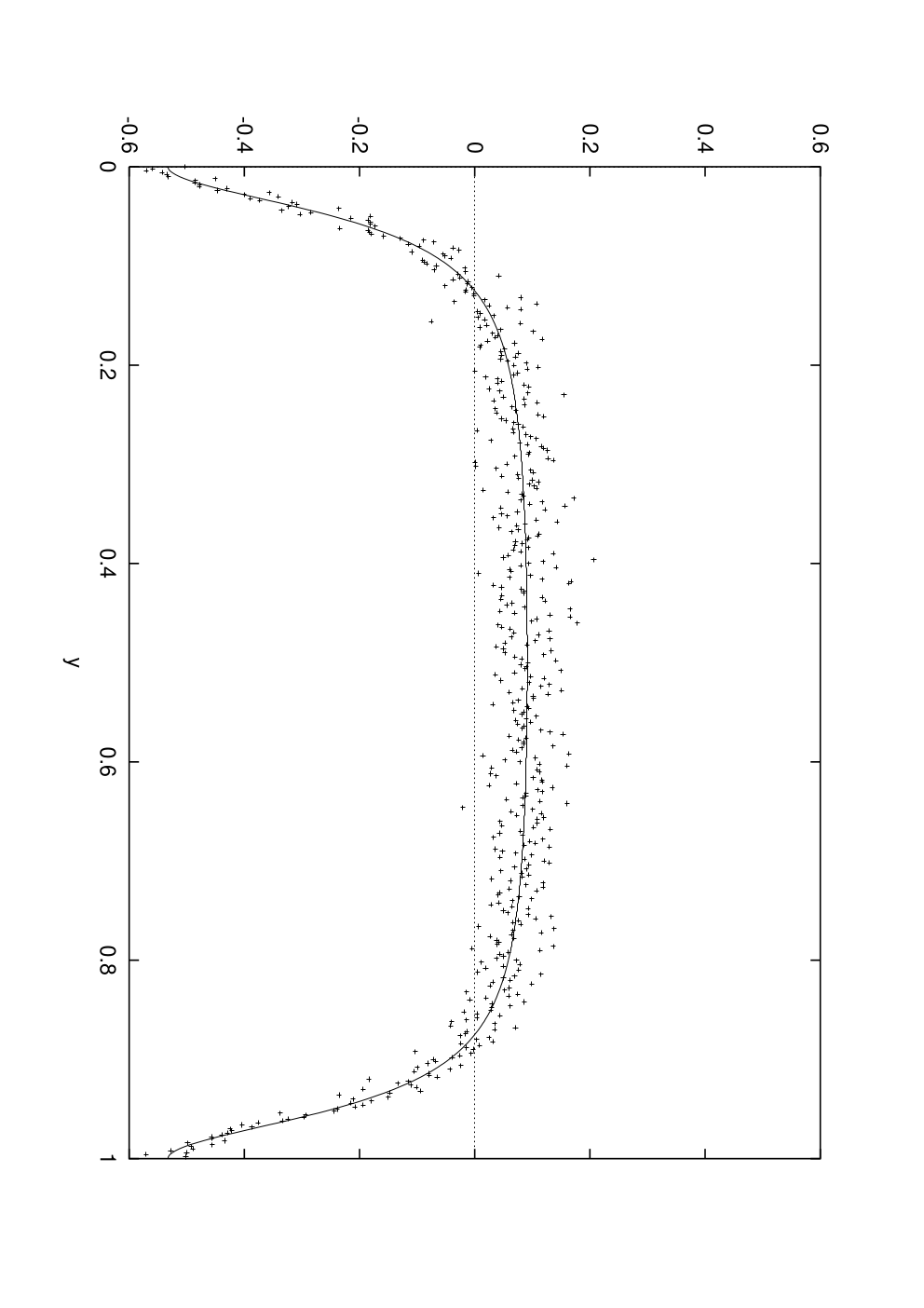
(1.10) $$\begin{split}g_{\alpha}(t)&=-\frac{\log p}{\pi}\Re\sum_{k=1}^{\infty}(p^{a/2}e^{2\pi iqt})^{-k}\\ &=-\frac{(p^{\frac{a}{2}}\cos 2\pi qt-1)\log p}{\pi(p^{a}-2p^{\frac{a}{2}}\cos 2\pi qt+1)}\,.\end{split}$$

As a function of $t$, $g_{\alpha}(t)$ attains its global minimum at each of the points $t=\frac{k}{q}$, $k=0,1,\cdots,q-1,$ the minimum being

(1.11) $$g_{\alpha}\Big(\frac{k}{q}\Big)=-\frac{\log p}{\pi(p^{\frac{a}{2}}-1)}<0.$$

In particular, this shows that there is a shortage of zeros of $\zeta(s)$ with imaginary parts $\gamma$ such that $\{\alpha\gamma\}=\{\frac{a\log p}{2\pi q}\gamma\}$ is close to one of the points $\frac{k}{q}$, $k=0,1,\ldots,q-1$. When $q=1$, this corresponds to Rademacher’s statement mentioned above.

We conclude this introduction by showing some histograms of $M(y;T)$ for $T=600,000$ ($N(T)=999508$) and a few values of $\alpha$. The list of zeros to this height were kindly supplied by Andrew Odlyzko. We partition $[0,1)$ into 500 subintervals of length $\frac{1}{500}$. In Figure 1 we plot for each subinterval $I=[y,y+\frac{1}{500})$ the value of $500(M(y+\frac{1}{500})-M(y))$ and also the graph of $g_{\alpha}(y)$.

$\displaystyle\alpha=\frac{\log 2}{2\pi}$

$\displaystyle\alpha=\frac{\log 5}{3\cdot 2\pi}$

$\displaystyle\alpha=\frac{\log 6}{2\pi}$

Figure 1. $500(M(y+\frac{1}{500})-M(y))$ vs. $g_{\alpha}(y)$ for $T=600000$.

2. Statement of results and conjectures

To state our main theorem, we consider for any $f\in L_{1}({\mathbb{T}})$ the modulus of continuity ([1], Definition 1.5.1)

$$\omega(f;\delta)=\sup_{|u|\leq\delta}\int_{\mathbb{T}}|f(t+u)-f(t)|\,dt.$$

For any real numbers $\alpha>0$ and $T>0$ define the measure $\mu_{\alpha,T}$ as in (1.3), and let $g_{\alpha}:{\mathbb{T}}\rightarrow{\mathbb{R}}$ be defined by (1.9) or (1.10), as appropriate.

Theorem 1.

Let $\alpha>0$ and let $h:{\mathbb{T}}\rightarrow{\mathbb{C}}$ be an absolutely continuous function with

(2.1) $$\omega(h^{\prime};\delta)=o(1/\log(1/\delta))\quad(\delta\to 0^{+}).$$

Then

(2.2) $$\lim_{T\rightarrow\infty}\int_{{\mathbb{T}}}hd\mu_{\alpha,T}=\int_{{\mathbb{T}}}hg_{\alpha}d\mu.$$

Corollary 2.

The equality (2.2) holds for all $h\in C^{2}({\mathbb{T}})$.

Proof.

Since $h\in C^{2}({\mathbb{T}})$,

$$\omega(h^{\prime};\delta)=\sup_{|u|\leq\delta}\int_{\mathbb{T}}\left|\int_{t}^{t+u}h^{\prime\prime}(y)\,dy\right|\,dt\leq\delta\int_{\mathbb{T}}|h^{\prime\prime}|=O(\delta).$$

∎

Corollary 3.

Suppose $\alpha=\frac{a\log p}{2\pi q}$, where $p$ is prime and $(a,q)=1$. Then

$$\int_{\mathbb{T}}|M(y;T)|\,dt\geq B(\alpha)+o(1),$$

where

$$B(\alpha)=\frac{\int_{\mathbb{T}}g_{\alpha}^{2}\,d\mu}{\max|g^{\prime}_{\alpha}|}.$$

Therefore, $D_{\alpha}^{*}(T)\geq\frac{B(\alpha)/2\pi+o(1)}{\log T}$ for these $\alpha$.

Proof.

Apply Theorem 1 with $h=g_{\alpha}$ (this may or may not be optimal). By integration by parts,

$$\begin{split}\left|\int_{\mathbb{T}}g_{\alpha}^{2}+o(1)\right|&=\left|\int_{\mathbb{T}}M(y;T)g_{\alpha}^{\prime}(y)\,dy\right|\\ &\leq\left(\int_{\mathbb{T}}|M(y;T)|\,dy\right)\max|g_{\alpha}^{\prime}(y)|.\end{split}$$

∎

Theorem 4.

Let $\alpha>0$ and suppose $D_{\alpha}^{*}(T)\ll\frac{1}{\log T}$. Then (2.2) holds for all absolutely continuous functions $h:{\mathbb{T}}\rightarrow{\mathbb{C}}$.

Corollary 5.

On RH, (2.2) holds for all absolutely continuous functions $h$ on ${\mathbb{T}}$.

Proof.

By Hlawka’s Theorem, if RH is true then $D_{\alpha}^{*}(T)\ll 1/\log T$. ∎

The main open problem in this line of investigation is to determine the largest “natural” class of functions for which (2.2) holds. We conjecture that (2.2) holds for the characteristic function of the interval $[0,y)$.

Conjecture A. If $\alpha=\frac{a\log p}{2\pi q}$, where $p$ is prime and $(a,q)=1$, then uniformly in $y$,

$$\lim_{T\to\infty}M(y;T)=\int_{0}^{y}g_{\alpha}(t)\,dt=-\frac{\log p}{2\pi^{2}q}\arg(1-p^{-a/2}e^{-2\pi iqy}).$$

When $\alpha$ is not of this form, $\lim_{T\to\infty}M(y,T)=0$ uniformly in $y$.

Corollary 6.

Assume Conjecture A. Suppose $\alpha=\frac{a\log p}{2\pi q}$, where $p$ is prime and $(a,q)=1$. As $T\to\infty$,

$$D_{\alpha}^{*}(T)=(1+o(1))\frac{\log p}{\pi q}\;\frac{\arcsin(p^{-a/2})}{\log T}.$$

When $\alpha$ is not of this form, $D_{\alpha}^{*}(T)=o(1/\log T)$.

In the opposite direction, (2.2) cannot hold for all functions $h$ which are continuous and differentiable on ${\mathbb{T}}$. This is a consequence of a property of general sequences (uniformly distributed or not), which we state below.

Theorem 7.

Let $a_{1},a_{2},\ldots$ be an arbitrary sequence of numbers in ${\mathbb{T}}$, let $t$ be a point in ${\mathbb{T}}$ and let $f(x)$ be a function decreasing monotonically to $0$ arbitrarily slowly. Then there is a function $h$, continuous and differentiable on ${\mathbb{T}}$, and which is $C^{\infty}({\mathbb{T}}\backslash\{t\})$, so that for an infinite set of $n\in{\mathbb{N}}$,

(2.3) $$\left|\frac{1}{n}\sum_{j=1}^{n}h(a_{j})-\int_{\mathbb{T}}h\right|\geq f(n).$$

In connection with his work on $k$-functions, Kaczorowski [8] was also led to study similar questions on the distribution of the imaginary parts of zeros of the zeta function and Dirichlet $L$-functions. In our terminology, his results concern the measures

$$\nu_{\alpha,n}=\frac{1}{n!}\sum_{\gamma>0}e^{-\gamma}\gamma^{n}\delta_{\{\alpha\gamma\}}-\frac{1}{n!}\sum_{\gamma>0}e^{-\gamma}\gamma^{n}\mu,$$

which essentially capture the distribution of $\{\alpha\gamma\}$ for $|\gamma-n|\ll\sqrt{n}$. Kaczorowski’s Conjecture A corresponds to our Corollary 6, and his Conjectures B, B₁ and B₂ to our Conjecture A.

We also mention that Fujii ([4], Theorem 5) has proved (2.2) in the special case $h(u)=B_{2}(u)=u^{2}-u+\frac{1}{6}$ (which is covered by Theorem 1) He has also proven, for a wide class of smooth functions $f$, that the sequence $\{f(\gamma)\}$ is uniformly distributed [2].

Lastly, we mention that analogs of our results should hold for a wide variety of $L$-functions, including Dirichlet $L$-functions. In deriving such results, the primary tools would be a generalization of Lemma 1 below and zero density estimates analogous to Lemma 2 below which are nontrivial for certain sequences of $\sigma,T$ with $T\to\infty$ and $\sigma-\frac{1}{2}\to 0^{+}$. This will be addressed in a future paper.

3. Proof of Theorem 1

Our principal tools are the following two lemmas.

Lemma 1.

Let $x,T>1,$ and denote by $n_{x}$ the nearest prime power to $x.$ Then

(3.1) $$\sum_{0<\gamma\leq T}x^{\rho}=-\frac{\Lambda(n_{x})}{2\pi}\frac{e^{iT\log(x/n_{x})}-1}{i\log(x/n_{x})}+O\left(x\log^{2}(2xT)+\frac{\log 2T}{\log x}\right),$$

where if $x=n_{x}$ the first term is $-T\frac{\Lambda(n_{x})}{2\pi}$.

This is a uniform version of a theorem of Landau [11], and the proof is nearly identical to the proof of Theorem 1 of Gonek ([5], §3). The only difference is in the treatment of the term $n=n_{x}$ occuring in Gonek’s integral $I_{1}$. That term is

$$V=-\frac{\Lambda(n_{x})}{2\pi}(x/n_{x})^{c}\int_{1}^{T}(x/n_{x})^{it}\,dt,\quad c=1+\frac{1}{\log(3x)}.$$

Gonek estimates this crudely as $V\ll\log x\min(T,x/|x-n_{x}|)$, but we are more precise. If $|x-n_{x}|\geq 1$, then $V\ll x\log(2x)$ and otherwise

$$\begin{split}V&=-\frac{\Lambda(n_{x})}{2\pi}(1+O(|x-n_{x}|/x))\left(\frac{e^{iT\log(x/n_{x})}-1}{i\log(x/n_{x})}+O(1)\right)\\ &=O(\log(2x))-\frac{\Lambda(n_{x})}{2\pi}\frac{e^{iT\log(x/n_{x})}-1}{i\log(x/n_{x})}.\end{split}$$

Let $N(\sigma,T)$ be the number of zeros $\rho=\beta+i\gamma$ of $\zeta(s)$ with $|\gamma|\leq T$ and $\beta\geq\sigma$. The following density bound is due to Selberg (Theorem 9.19C of [18]).

Lemma 2.

Uniformly in $\frac{1}{2}\leq\sigma\leq 1$, we have $N(\sigma,T)\ll T^{1-\frac{1}{4}(\sigma-1/2)}\log T$.

We now proceed with the proof of Theorems 1 and 4. Fix $\alpha>0$ and an absolutely continuous function $h:{\mathbb{T}}\rightarrow{\mathbb{C}}$. In what follows, constants implied by the $O-$ and $\ll-$symbols may depend on $\alpha$ and $h$. Suppose either $D_{\alpha}^{*}(T)\ll 1/\log T$ or $h$ satisfies (2.1). Looking at the definition of $\mu_{\alpha,T}$ we see that what we need to show in order to complete the proof of the theorems is that

(3.2) $$\frac{1}{T}\sum_{0<\gamma\leq T}h(\alpha\gamma)-\frac{N(T)}{T}\int_{0}^{1}h(u)du=\int_{0}^{1}h(u)g_{\alpha}(u)\,du+o(1)$$

as $T\rightarrow\infty.$ By treating separately the real part and the imaginary part of $h,$ we may assume in what follows that $h$ is real. We start by approximating $h$ by a trigonometric polynomial based on its Fourier series

(3.3) $$h(u)=\sum_{m\in{\mathbb{Z}}}c_{m}e^{2\pi mui},$$

where the Fourier coefficients $c_{m}$ are given by

(3.4) $$c_{m}=\int_{0}^{1}h(u)e^{-2\pi mui}\,du.$$

Since $h$ is absolutely continuous, we have $h^{\prime}\in L_{1}({\mathbb{T}})$ and consequently by the Riemann-Lebesgue Lemma,

(3.5) $$c_{m}=o(1/m)\qquad(m\to\infty).$$

Let

$$K_{J}(u)=\frac{3}{J(2J^{2}+1)}\left(\frac{\sin\pi Ju}{\sin\pi u}\right)^{4}=\frac{3}{J(2J^{2}+1)}\biggl(\sum_{k=0}^{J-1}e^{(1-J+2k)u\pi i}\biggr)^{4}$$

be the Jackson kernel ([1], Problem 1.3.9) and define

$$H_{J}(y)=\int_{{\mathbb{T}}}K_{J}(u)h(u-y)\,du=\sum_{|j|\leq 2J}A^{(J)}_{j}c_{j}e^{2\pi jui},$$

where

$$A^{(J)}_{0}=1,\quad|A^{(J)}_{j}|\leq 1,\quad\lim_{J\to\infty}A^{(J)}_{j}=1\text{ for each fixed }j.$$

This kernel is chosen because it provides a very fast rate of $L_{1}({\mathbb{T}})$-convergence of $H_{J}$ to $h$ (see [1], §1.6 and Ch. 2 for more on this subject). The same is true for the convergence of $H_{J}^{\prime}$ to $h^{\prime}$. Specifically, we have ([1], Lemma 1.5.4, Theorem 1.5.8 and Corollary 1.5.9)

(3.6) $$\int_{\mathbb{T}}|H_{J}^{\prime}-h^{\prime}|=O(\omega(h^{\prime};1/J)).$$

Let $T$ be a large real number. Applying integration by parts to the left side of (2.2) and using (1.4) and (1.5), we obtain

(3.7) $$\begin{split}\int_{{\mathbb{T}}}hd\mu_{\alpha,T}&=\int_{\mathbb{T}}h(y)\,dM(y;T)\\ &=\int_{\mathbb{T}}H_{J}(y)\,dM(y;T)+\int_{\mathbb{T}}(h(y)-H_{J}(y))\,dM(y;T)\\ &=\int_{\mathbb{T}}H_{J}(y)\,dM(y;T)-\int_{\mathbb{T}}M(y;T)\,(h^{\prime}(y)-H_{J}^{\prime}(y))\,dy\\ &=\frac{1}{T}\sum_{1\leq|j|\leq 2J-2}A^{(J)}_{j}c_{j}\sum_{0<\gamma\leq T}x_{j}^{i\gamma}+O\left(D^{*}(T)\log T\int_{\mathbb{T}}|h^{\prime}-H_{J}^{\prime}|\right),\end{split}$$

where we have written $x_{j}=e^{2\pi j\alpha}$.

To apply Lemma 1, we write $x^{i\gamma}=x^{\rho-1/2}+x^{i\gamma}(1-x^{\beta-1/2})$. Let $\delta=50\frac{\log\log T}{\log T}$. Assume that

$$0<\delta\log x<1.$$

Note that if $\beta+i\gamma$ is a zero, then $1-\beta+i\gamma$ is also a zero. We obtain from Lemma 2 the bounds

$$\sum_{\begin{subarray}{c}0<\gamma\leq T\\ |\beta-\frac{1}{2}|\geq\delta\end{subarray}} x^{i\gamma}(1-x^{\beta-1/2})\ll\sum_{\begin{subarray}{c}0<\gamma\leq T\\ \beta\geq\frac{1}{2}+\delta\end{subarray}}x^{\beta-1/2}$$

$$\ll x^{\delta}N(1/2+\delta,T)+\log x\int_{1/2+\delta}^{1}x^{\sigma-1/2}N(\sigma,T)\,d\sigma$$

$$\ll T\log T\biggl[T^{-\delta/4}+\log x\int_{\delta}^{1/2}\left(\frac{T^{1/4}}{x}\right)^{\theta}\,d\theta\biggr]$$

$$\ll\frac{T}{\log^{10}T}$$

and

$$\sum_{\begin{subarray}{c}0<\gamma\leq T\\ |\beta-\frac{1}{2}|<\delta\end{subarray}}x^{i\gamma}(1-x^{\beta-1/2}) \ll\sum_{\begin{subarray}{c}0<\gamma\leq T\\ \frac{1}{2}<\beta<\frac{1}{2}+\delta\end{subarray}}(x^{\beta-1/2}+x^{1/2-\beta}-2)$$

$$\ll\log^{2}x\sum_{\begin{subarray}{c}0<\gamma\leq T\\ \frac{1}{2}<\beta<\frac{1}{2}+\delta\end{subarray}}(\beta-1/2)^{2}$$

$$\ll\log^{2}x\int_{0}^{\delta}\theta N(1/2+\theta,T)\,d\theta$$

$$\ll\frac{T\log^{2}x}{\log T}.$$

Thus

(3.8) $$\sum_{0<\gamma\leq T}(x^{i\gamma}-x^{\rho-1/2})\ll\frac{T\log^{2}x}{\log T}.$$

We apply these estimates with $x=x_{j}$, $1\leq j\leq 2J-2$, noting that $x_{-j}^{i\gamma}=x_{j}^{-i\gamma}$ and $c_{-j}=\overline{c_{j}}$. By Lemma 1, we obtain

(3.9) $$\begin{split}\int_{{\mathbb{T}}}&hd\mu_{\alpha,T}=-\frac{1}{\pi}\Re\left[\sum_{j=1}^{2J-2}\frac{A^{(J)}_{j}c_{j}\Lambda(n_{x_{j}})}{\sqrt{x_{j}}}\frac{\sin\left(T\log(x_{j}/n_{x_{j}})\right)}{T\log(x_{j}/n_{x_{j}})}\right]\\ &\qquad+O\left(\frac{1}{T}\sum_{j=1}^{2J-2}|c_{j}|x_{j}^{1/2}\log^{2}(2x_{j}T)+\frac{1}{\log T}\sum_{j=1}^{2J-2}|c_{j}|\log^{2}x_{j}\right)\\ &\qquad+O\left(D^{*}(T)\log T\int_{\mathbb{T}}|h^{\prime}-H_{J}^{\prime}|\right).\end{split}$$

Now put

(3.10) $$J=\lfloor(\log T)^{1/3}+1\rfloor.$$

Using (3.5), (3.10) and $\log x_{j}=O(j)$, we find that the first error term in (3.9) is

$$O\left(\frac{x_{2J-2}^{1/2}\log^{2}T}{T}+\frac{J^{2}}{\log T}\right)=o(1)\quad(T\to\infty).$$

We now estimate the second error term in (3.9). Since $h^{\prime}\in L_{1}({\mathbb{T}})$, $\int_{\mathbb{T}}|h^{\prime}-H_{J}^{\prime}|\to 0$ as $J\to\infty$. Thus, if $D_{\alpha}^{*}(T)\ll 1/\log T$, then

(3.11) $$D^{*}(T)\log T\int_{\mathbb{T}}|h^{\prime}-H_{J}^{\prime}|=o(1).$$

Similarly, (3.11) follows if (2.1) holds by (3.6).

Consider now the main term in (3.9). This sum is absolutely and uniformly convergent in $T$ and each term with $n_{x_{j}}\neq x_{j}$ tends to zero as $T\to\infty$. Thus, the aggregate of such terms is $o(1)$ as $T\to\infty$. Therefore, by (3.8) and (3.11),

$$\int_{{\mathbb{T}}}hd\mu_{\alpha,T}=-\frac{1}{\pi}\Re\left[\sum_{j=1}^{2J-2}\frac{A^{(J)}_{j}c_{j}\Lambda(x_{j})}{\sqrt{x_{j}}}\right]+o(1)\quad(T\to\infty).$$

In the case where $\alpha$ is not of the form $\frac{a}{q}\frac{\log p}{2\pi}$ for positive integers $a,q$ and prime $p$, $\Lambda(x_{j})=0$ for all $j$ and this finishes the proof. If $\alpha$ does have this form, $\Lambda(x_{j})=0$ unless $q|j$, in which case $\Lambda(x_{j})=\log p$. Thus

$$\int_{{\mathbb{T}}}hd\mu_{\alpha,T}=-\frac{\log p}{\pi}\Re\left[\sum_{m\leq(2J-2)/q}\frac{A^{(J)}_{qm}c_{qm}}{p^{am/2}}\right]+o(1)\quad(T\to\infty).$$

It is easily seen that (since $h$ and $g_{\alpha}$ are absolutely continuous) that the right side approaches $\int hg_{\alpha}$ as $T\to\infty$. This completes the proof of Theorem 1.

4. Proof of Theorem 7

First, if $a_{1},a_{2},\ldots$ is not uniformly distributed in $[0,1)$, by Weyl’s criterion the conclusion of Theorem 6 holds with $h(y)=e^{2\pi iky}$ for some integer $k$, regardless of the function $f$.

From now on assume that $a_{1},a_{2},\ldots$ is uniformly distributed in $[0,1)$. Let $r(x)$ be a $C^{\infty}({\mathbb{R}})$ function such that $r(x)=0$ for $|x|\geq 1/2$, $r(0)=1$ and $r$ is monotone on $[-1/2,0]$ and $[0,1/2]$. For any real number $u$, and any $v>0$, $\delta>0$, denote by $r_{u,v,\delta}$ the function defined by

$$r_{u,v,\delta}(x)=vr\left(\frac{x-u}{\delta}\right),\,\,\,x\in{\mathbb{R}}.$$

Thus $r_{u,v,\delta}$ is nonnegative, is $C^{\infty}({\mathbb{R}})$, it is supported on an interval of length $\delta$ centered at $u$, and one has $r_{u,v,\delta}(u)=v$. Note also that

$$\int_{{\mathbb{R}}}r_{u,v,\delta}(x)dx=v\delta\int_{{\mathbb{R}}}r(x)dx.$$

We now proceed to construct a function $h$ as in the statement of the theorem. It is enough to define $h$ on the interval $(t-1,t]$. We set $h(t)=0$. Next, we write the interval $(t-1,t)$ as a disjoint union of intervals

$$I_{k}=\left(t-\frac{1}{2^{k-1}},t-\frac{1}{2^{k}}\right],\,\,\,k=1,2,3,\dots,$$

and we define $h$ inductively on each of the intervals $I_{k}$. We also set

$$J_{k}=\left[t-\frac{7}{2^{k+2}},t-\frac{5}{2^{k+2}}\right]$$

for any $k\geq 1$. Thus $J_{k}$ is contained in $I_{k}$ and length $(J_{k})=1/2^{k+1}$. For each $k\geq 1$, we will select a positive integer $n_{k}$, and two real numbers $v_{k}>0$, $\delta_{k}>0$. Then $h$ will be defined on $I_{k}$ by

(4.1) $$h(x)=\sum_{\begin{subarray}{c}a_{n}\in J_{k}\\ n\leq n_{k}\end{subarray}}r_{a_{n},v_{k},\delta_{k}}(x).$$

Here the sum is restricted to distinct values of $a_{n}$. Thus if $a_{n}$ is the same for several values of $n\leq n_{k}$, only one of these values of $n$ is taken on the right side of (4.1). We will choose $\delta_{k}$ to be smaller than $1/2^{k+2}$. Then the right side of (4.1) will indeed be supported inside the interval $I_{k}$. Moreover, $h$ will vanish on a small interval around each of the points $t-\frac{1}{2^{k}}$ with $k\geq 1$. Note also that on each $I_{k}$, $h$ is a finite sum of $C^{\infty}$ functions, so after this construction is complete $h$ will be $C^{\infty}$ on ${\mathbb{T}}\setminus\{t\}$. For each $k$, we only choose $\delta_{k}$ after $n_{k}$ has already been chosen. Then we let $\delta_{k}$ to be small enough so that $|a_{n}-a_{n^{\prime}}|>\delta_{k}$ for any $n,n^{\prime}\leq n_{k}$ with $a_{n^{\prime}}\neq a_{n}$. This will make the supports of the functions $r_{a_{n},v_{k},\delta_{k}}$ from the right side of (4.1) to be disjoint. As a consequence, one will have $0\leq h(x)\leq v_{k}$ for any $x\in I_{k}$. If we choose the sequence $(v_{k})_{k\geq 1}$ to be decreasing to $0$, the function $h$ will be continuous at $t$. If furthermore the sequence $(v_{k})_{k\geq 1}$ is chosen so that

$$\lim_{k\rightarrow\infty}2^{k}v_{k}=0,$$

then $h$ will be differentiable at $t$, and $h^{\prime}(t)=0$. We put $v_{k}=1/3^{k}$, so the above condition holds. It remains to construct the sequences $(n_{k})_{k\geq 1}$, and $(\delta_{k})_{k\geq 1}$. Fix a $k$ and assume that $n_{j}$ and $\delta_{j}$ have already been defined for $j=1,\dots,k-1$. This means that $h$ has been constructed on the interval $E_{k}:=I_{1}\cup\dots\cup I_{k-1}$. Let $n_{k}^{\prime}$ be such that for any $n\geq n_{k}^{\prime}$ we have $f(n)<1/7^{k}$. Now, since the sequence $(a_{n})_{n\geq 1}$ is uniformly distributed, there exists an $n_{k}^{\prime\prime}$ such that for any $n\geq n_{k}^{\prime\prime}$ one has

$$\left|\frac{1}{n}\sum_{\begin{subarray}{c}1\leq j\leq n\\ a_{j}\in E_{k}\end{subarray}}h(a_{j})-\int_{E_{k}}h\right|\leq\frac{1}{7^{k}}.$$

The fact that $(a_{n})_{n\geq 1}$ is uniformly distributed also implies the existence of an $n_{k}^{\prime\prime\prime}$ such that for any $n\geq n_{k}^{\prime\prime\prime}$,

$$\#\{m\leq n:a_{m}\in J_{k}\}>\frac{n}{2^{k+2}}\,.$$

We put $n_{k}=\max\{n_{k}^{\prime},n_{k}^{\prime\prime},n_{k}^{\prime\prime\prime}\}$. Then by the above it follows that

$$f(n_{k})<\frac{1}{7^{k}}\,,$$

$$\left|\frac{1}{n_{k}}\sum_{\begin{subarray}{c}1\leq j\leq n_{k}\\ a_{j}\in E_{k}\end{subarray}}h(a_{j})-\int_{E_{k}}h\right|\leq\frac{1}{7^{k}}\,,$$

and

$$\frac{1}{n_{k}}\sum_{\begin{subarray}{c}1\leq j\leq n_{k}\\ a_{j}\in I_{k}\end{subarray}}h(a_{j})\geq\frac{\#\{j\leq n_{k}:a_{j}\in J_{k}\}}{n_{k}}v_{k}\geq\frac{1}{2^{k+2}3^{k}}\,.$$

Lastly, we choose $\delta_{k}>0$ to be small enough so that it satisfies all the requirements stated so far, and such that we also have

$$\int_{I_{k}}h<\frac{1}{7^{k}}.$$

This completes the construction of the three sequences $(n_{k})_{k\geq 1}$, $(v_{k})_{k\geq 1}$, $(\delta_{k})_{k\geq 1}$, and thus also the construction of $h$. It remains to check that the inequality from the statement of the theorem holds for infinitely many $n$. Take $n=n_{k}$, and break the interval $(t-1,t]$ as a disjoint union of three intervals, $(t-1,t]=E_{k}\cup I_{k}\cup T_{k}$, where $T_{k}=(t-1/2^{k},t]$. We also break accordingly the sum and the integral from (2.3),

$$\frac{1}{n_{k}}\sum_{j=1}^{n_{k}}h(a_{j})=\Sigma_{E_{k}}+\Sigma_{I_{k}}+\Sigma_{T_{k}},$$

and respectively

$$\int_{\mathbb{T}}h=\int_{E_{k}}h+\int_{I_{k}}h+\int_{T_{k}}h.$$

We know that $\left|\Sigma_{E_{k}}-\int_{E_{k}}h\right|\leq 1/7^{k}$, $\Sigma_{I_{k}}\geq 1/(4\cdot 6^{k})$, $0<\int_{I_{k}}h\leq 1/7^{k}$ and $f(n_{k})\leq 1/7^{k}$. Also $\Sigma_{T_{k}}\geq 0$, and since for any $m>k$ we have $0\leq\int_{I_{m}}h\leq 1/7^{m}$, it follows that $\int_{T_{k}}h<2/7^{k}$. We conclude that for large $k$,

$$\frac{1}{n_{k}}\sum_{j=1}^{n_{k}}h(a_{j})-\int_{\mathbb{T}}h\geq\frac{1}{4\cdot 6^{k}}-\frac{4}{7^{k}}\geq f(n_{k}),$$

which completes the proof of the theorem.

References

• [1] P. L. Butzer and R. J. Nessel, Fourier analysis and approximation, vol. 1, Academic Press, New York, 1971.
• [2] A. Fujii, On the uniformity of the distribution of the zeros of the Riemann zeta function, J. reine angew. Math. 302 (1978), 167–205.
• [3] A. Fujii, Some problems of Diophantine approximation in the theory of the Riemann zeta function (III), Comment. Math. Univ. St. Pauli 42 (1993), 161–187.
• [4] A. Fujii, Some problems of Diophantine approximation in the theory of the Riemann zeta function (IV), Comment. Math. Univ. St. Pauli 43 (1994), 217–244.
• [5] S. M. Gonek, An explicit formula of Landau and its applications to the theory of the zeta-function, A tribute to Emil Grosswald: number theory and related analysis, Contemp. Math., 143, Amer. Math. Soc., Providence, RI (1993), 395–413.
• [6] D. Hejhal, On the triple correlation of the zeros of the zeta function, Int. Math. Res. Not. (1994), 293–302.
• [7] E. Hlawka, Über die Gleichverteilung gewisser Folgen, welche mit den Nullstellen der Zetafunktionen zusammenhängen, Sitzungsber. Österr. Akad. Wiss., Math.–Naturw. Kl. Abt. II 184 (1975), 459–471.
• [8] J. Kaczorowski, The kk-functions in multiplicative number theory, III. Uniform distribution of zeta zeros; discrepancy, Acta Arith. 57 (1991), 199–210.
• [9] N. M. Katz, P. Sarnak, Zeroes of zeta functions and symmetry, Bull. Amer. Math. Soc. (N. S.) 36 (1999), no 1, 1–26.
• [10] L. Kuipers and H. Niederreiter, Uniform distribution of sequences, New York 1974.
• [11] E. Landau. Über die Nullstellen der ζ\zeta-Funktion, Math. Ann. 71 (1911), 548–568.
• [12] H. L. Montgomery, The pair correlation of zeros of the zeta function, Proc. Sym. Pure Math. 24 (1973), 181–193.
• [13] M. R. Murty, A. Perelli, The Pair Correlation of Zeros of Functions in the Selberg Class, Int. Math. Res. Not. 10 (1999) 531–545.
• [14] M. R. Murty, A. Zaharescu, Explicit formulas for the pair correlation of zeros of functions in the Selberg class, Forum Math. 14 (2002), no. 1, 65–83.
• [15] A. M. Odlyzko, On the distribution of spacings between zeros of the zeta function, Math. Comp. 48 (1987), 273–308.
• [16] H. Rademacher, Fourier analysis in number theory, Symposium on harmonic analysis and related integral transforms: Final technical report, Cornell Univ., Ithica, N.Y. (1956), 25 pages; also in: H. Rademacher, Collected Works, pp. 434–458.
• [17] Z. Rudnick, P. Sarnak, Principal LL-functions and Random Matrix Theory, Duke Math. J. 81, 2 (1996), 269–322.
• [18] E. C. Titchmarsh, The Theory of the Riemann Zeta-function, 2nd ed. rev. by D. R. Heath-Brown, Clarendon Press, Oxford 1986.