Asymptotic zero behavior of Laguerre polynomials with negative parameter

Abstract

We consider Laguerre polynomials $L_{n}^{(\alpha_{n})}(nz)$ with varying negative parameters $\alpha_{n}$, such that the limit $A=-\lim_{n}\alpha_{n}/n$ exists and belongs to $(0,1)$. For $A>1$, it is known that the zeros accumulate along an open contour in the complex plane. For every $A\in(0,1)$, we describe a one-parameter family of possible limit sets of the zeros. Under the condition that the limit $r=-\lim_{n}\frac{1}{n}\log\left[{\rm dist\,}(\alpha_{n},\mathbb{Z})\right]$ exists, we show that the zeros accumulate on $\Gamma_{r}\cup[\beta_{1},\beta_{2}]$ with $\beta_{1}$ and $\beta_{2}$ only depending on $A$. For $r\in[0,\infty)$, $\Gamma_{r}$ is a closed loop encircling the origin, which for $r=+\infty$, reduces to the origin. This shows a great sensitivity of the zeros to $\alpha_{n}$’s proximity to the integers.

We use a Riemann-Hilbert formulation for the Laguerre polynomials, together with the steepest descent method of Deift and Zhou to obtain asymptotics for the polynomials, from which the zero behavior follows.

1 Introduction

The zeros of Laguerre polynomials $L_{n}^{(\alpha)}$ with negative parameters $\alpha$ have a remarkable behavior. For $\alpha>-1$, these polynomials are orthogonal with respect to the weight $x^{\alpha}e^{-x}$ on $[0,\infty)$, and the zeros are all real and positive. This is no longer true if $\alpha<-1$. The explicit representation, see [31],

$$L_{n}^{(\alpha)}(z)=\sum_{k=0}^{n}\binom{n+\alpha}{n-k}\frac{(-z)^{k}}{k!}$$ (1.1)

shows that $L_{n}^{(\alpha)}$ has a zero of order $|\alpha|$ at $0$ if $\alpha$ is an integer in $\{-n,-n+1,\ldots,-1\}$. For these values of $\alpha$ we have

$$L_{n}^{(\alpha)}(z)=\frac{(n+\alpha)!}{n!}(-z)^{-\alpha}L_{n+\alpha}^{(-\alpha)}(z).$$ (1.2)

This means that in addition to the $|\alpha|$ zeros at $0$, there are $n-|\alpha|$ zeros in $(0,\infty)$. For a non-integer $\alpha\in(-n,-1)$ it is known that there are exactly $n-[-\alpha]$ positive zeros and for $\alpha<-n$ there are no positive zeros at all, see [31, §6.73]. In all cases there is at most one negative real zero.

Non-trivial limiting behavior takes place for the zeros of scaled Laguerre polynomials $L_{n}^{(\alpha_{n})}(nz)$ with varying negative parameters $\alpha_{n}$ such that the limit

$$\lim_{n\to\infty}-\frac{\alpha_{n}}{n}=A>0$$ (1.3)

exists. The asymptotic location of the zeros depends on $A$ as shown in Figure 1 which is taken from [21], see also [25]. See [26] for analogous plots of zeros of Jacobi polynomials with negative parameters.

Figure 1: Zeros of Laguerre polynomials $L_{n}^{(-nA)}(nz)$ for $n=40$ and $A=0.81$ (left), $A=1.01$ (middle), and $A=2$ (right).

From the plots in Figure 1 it seems clear that the zeros accumulate along certain contours in the complex plane. For $A>1$, the contour is an open arc, while for $0<A<1$, the contour consists of a closed loop together with an interval on the positive real axis. In the intermediate case $A=1$, the contour is a simple closed contour.

The case $A>1$ is well-understood. Indeed, Saff and Varga [29] showed that all of the zeros accumulate on a well-defined open arc. Saff and Varga stated their results in terms of the zeros of the numerator and denominator polynomials of Padé approximants to the exponential functions, but these polynomials can be identified as Laguerre polynomials with integer parameters less than $-n$. Uniform asymptotics for the Laguerre polynomials $L_{n}^{(\alpha_{n})}(nz)$ in case $A>1$ were obtained more recently in [14], [21], and [32].

The case $0<A<1$ is less well-understood. The asymptotic expansion of Dunster [14] is also valid for this case, but his results on zeros are restricted to the case $A>1$. Martínez et al. [25] conjectured that if $(\alpha_{n})$ is a sequence of non-integers such that the limit (1.3) exists with $0<A<1$, then the zeros of the polynomials $L_{n}^{(\alpha_{n})}(nz)$ accumulate on a well-defined contour which they identify as a trajectory of a quadratic differential. As stated this conjecture is not true. Indeed, if every $\alpha_{n}$ is an integer, then there are $|\alpha_{n}|$ zeros at the origin. Since the zeros depend continuously on the parameter, it will follow that also for $\alpha_{n}$ very close to the integers, some of the zeros of the polynomials $L_{n}^{(\alpha_{n})}(nz)$ are still close to the origin. However, as we will show, the conjecture in [25] is true provided the distance of the parameters $\alpha_{n}$ to the integers is not exponentially small as $n\to\infty$.

It is the purpose of this paper to study the possible limiting behaviors of the zeros of $L_{n}^{(\alpha_{n})}(nz)$ as $n\to\infty$ such that (1.3) holds with $A\in(0,1)$. We define

$$\beta_{1}=2-A-2\sqrt{1-A},\qquad\beta_{2}=2-A+2\sqrt{1-A}.$$ (1.4)

and

$$R(z)=(z-\beta_{1})^{1/2}(z-\beta_{2})^{1/2},\qquad z\in\mathbb{C}\setminus[\beta_{1},\beta_{2}],$$ (1.5)

where the branches of the square roots are chosen so that $R(z)\sim z$ as $z\to\infty$. We also put

$$\phi(z)=\frac{1}{2}\int_{\beta_{1}}^{z}\frac{R(s)}{s}\;ds,\qquad z\in\mathbb{C}\setminus\left((-\infty,0]\cup[\beta_{1},\infty)\right),$$ (1.6)

where the path of integration from $\beta_{1}$ to $z$ lies entirely in $\mathbb{C}\setminus\left((-\infty,0]\cup[\beta_{1},\infty)\right)$ except for the initial point $\beta_{1}$.

Due to the pole of $R(s)/s$ at $s=0$ with residue $R(0)=-A$, the $\phi$ function has a jump on the negative real axis,

$$\phi_{+}(x)-\phi_{-}(x)=-A\pi i,\qquad x\in(-\infty,0),$$ (1.7)

where $\phi_{+}$ and $\phi_{-}$ denote the limits from above and below, respectively. In view of (1.7), ${\rm Re\,}\phi$ is a well-defined harmonic function on $\mathbb{C}\setminus\left(\{0\}\cup[\beta_{1},\infty)\right)$.

Theorem 1.1

For every $r\geq 0$, the following hold.

1. There exists a simple closed curve $\Gamma_{r}\subset\mathbb{C}\setminus\left(\{0\}\cup(\beta_{1},\infty)\right)$ encircling $0$ once in the clockwise direction, so that

   $${\rm Re\,}\phi(z)=r/2\qquad\mbox{for }z\in\Gamma_{r}.$$

2. The (a priori complex) measure

   $$d\nu_{r}(s)=\frac{1}{2\pi i}\frac{R(s)}{s}ds\qquad\mbox{ on }\Gamma_{r}$$

   where $\Gamma_{r}$ is oriented clockwise, is a positive measure with total mass $A$.

3. The measure

   $$d\mu_{r}=d\nu_{r}+\frac{\sqrt{(x-\beta_{1})(\beta_{2}-x)}}{2\pi x}\chi_{[\beta_{1},\beta_{2}]}(x)dx$$ (1.8)

   is a probability measure on $\Gamma_{r}\cup[\beta_{1},\beta_{2}]$.

Some of the contours $\Gamma_{r}$ are shown in Figure 2 together with the interval $[\beta_{1},\beta_{2}]$.

Figure 2: The interval $[\beta_{1},\beta_{2}]$ and some of the contours $\Gamma_{r}$ for the value $A=0.99$.

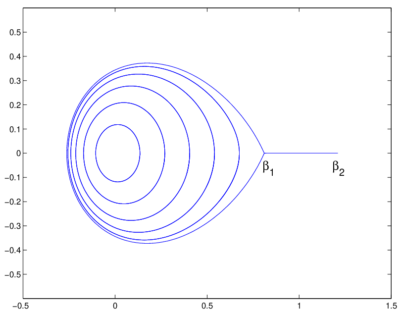
Now we consider a sequence $L_{n}^{(\alpha_{n})}(nz)$ of rescaled Laguerre polynomials with varying parameters $\alpha_{n}$ such that (1.3) holds with $A\in(0,1)$. We say that the zeros accumulate on a compact set $K$ if for every open set $\Omega\supset K$, there is $n_{0}$ such that for every $n\geq n_{0}$, all zeros of $L_{n}^{(\alpha_{n})}(nz)$ are contained in $\Omega$. We say that a probability measure $\mu$ is the asymptotic zero distribution if

$$\lim_{n\to\infty}\frac{1}{n}\sum_{j=1}^{n}\delta_{z_{j,n}}=\mu$$

in the sense of weak^∗ convergence of measures, see e.g. [28]. Here $z_{1,n},\ldots,z_{n,n}$ are the zeros of $L_{n}^{(\alpha_{n})}(nz)$, counted according to multiplicity, and $\delta_{z}$ is the unit Dirac measure at $z$.

Theorem 1.2

Let $(\alpha_{n})$ be a sequence such that the limit (1.3) holds with $A\in(0,1)$. Suppose that the limit

$$L=\lim_{n\to\infty}\left[{\rm dist\,}(\alpha_{n},\mathbb{Z})\right]^{1/n}$$ (1.9)

exists. Then the following hold.

1. If $L=0$, then the zeros of $L_{n}^{(\alpha_{n})}(nz)$ accumulate on $\{0\}\cup[\beta_{1},\beta_{2}]$ and

   $$A\delta_{0}+\frac{\sqrt{(x-\beta_{1})(\beta_{2}-x)}}{2\pi x}\chi_{[\beta_{1},\beta_{2}]}(x)dx$$ (1.10)

   is the asymptotic zero distribution.

2. If $L=e^{-r}$ with $0\leq r<\infty$, then the zeros of $L_{n}^{(\alpha_{n})}(nz)$ accumulate on $\Gamma_{r}\cup[\beta_{1},\beta_{2}]$ and the measure $\mu_{r}$ given in (1.8) is the asymptotic zero distribution.

Remark 1.3

The case $L=1$ in Theorem 1.2 represents the typical case, in the sense that if a sequence $(\alpha_{n})$ would be chosen randomly according to some reasonable distribution, then then

$$\lim_{n\to\infty}\left[{\rm dist\,}(\alpha_{n},\mathbb{Z})\right]^{1/n}=1$$

with probability one. So in the typical case, the zeros cluster on $[\beta_{1},\beta_{2}]$ and along the outer curve $\Gamma_{0}$. The case of limit $L<1$ in (1.9) is more special, since for that to happen the parameters $\alpha_{n}$ should be very close to integers.

To illustrate this, we have plotted in Figure 3 the zeros of $L_{n}^{(-nA)}$ with $n=40$, for the values $A=0.81$ and $A=0.799999975$. Then the distance of $\alpha_{n}=-nA$ to the integers is $0.4$ and $10^{-6}$, respectively. There is a clear separation in the plot on the right between the zeros on the interval $[\beta_{1},\beta_{2}]$ and the cluster of zeros around the origin. For the plot on the right, $\beta_{1}=0.31\cdots$ and $\beta_{2}=2.09\cdots$. The rightmost zero in the cluster has real part $0.14\cdots$.

  

Figure 3: Zeros of Laguerre polynomials $L_{n}^{(-nA)}(nz)$ for $n=40$ and $A=0.81$ (left), $A=0.799999975$ (right). The two cases correspond to ${\rm dist\,}(\alpha_{n},\mathbb{Z})=0.4$ and ${\rm dist\,}(\alpha_{n},\mathbb{Z})=10^{-6}$, respectively.

Remark 1.4

Theorem 1.2 also applies to subsequences. So, if $(\alpha_{n})$ is a sequence such that the limit (1.9) does not exist, then we can pass to a subsequence such that (1.9) exists along that subsequence. Then we find an asymptotic distribution of zeros for any subsequence such that the limit (1.9) exists. By constructing special sequences we can arrange it that different subsequences have different asymptotic zero distributions, and it is even possible to construct examples in which every measure $\mu_{r}$ appears as the asymptotic zero distribution along some subsequence.

Remark 1.5

For fixed $n$ and decreasing $\alpha<0$, the dynamics of the zeros of $L_{n}^{(\alpha)}$ is similar to the dynamics of the zeros of certain hypergeometric polynomials studied recently by Driver and Duren [12, 13]. For the Laguerre polynomials, the zeros are all real and positive if $\alpha>-1$. For $\alpha=-1$, there is one zero at the origin. This zero becomes negative if $\alpha$ becomes smaller than $-1$. As $\alpha$ decreases, the smallest zero reaches a minimum and then starts to increase again. For $\alpha=-2$, it is at the origin again, and simultaneously the second smallest zero has reached the origin. A collision takes place, and for $\alpha$ somewhat smaller than $-2$, the two zeros separate and leave the real axis, moving into the complex plane. When $\alpha$ has reached the next integer value $-3$ they both return to the origin, and a third zero coming from the positive real axis joins them in a three-fold collision. As $\alpha$ decreases from $-3$ to $-4$, the three zeros move into the complex plane, one on the negative real axis, and two away from the axis, coming again to the origin for a new collision at $\alpha=-4$, where they are joined by another zero coming from the positive real axis. And so on, until all $n$ zeros have left the positive real axis. At $\alpha=-n$, all $n$ zeros meet at the origin. For $\alpha<-n$, they separate again, and they all move into the complex plane. If $n$ is odd, then one zero remains on the negative real axis.

Remark 1.6

In statistical literature, see [2, 10] and the references cited therein, the measure (1.10) is known as the Marchenko-Pastur distribution [24]. It appears as the limiting spectral distribution of Wishart matrices, which are random covariance matrices $\frac{1}{p}XX^{T}$ where $X$ is an $n\times p$ matrix with independent, identically distributed entries. The measure (1.10) corresponds to the limit $n,p\to\infty$, $n/p\to 1-A\in(0,1)$.

In the theory of free probability, the measure (1.10) is also known as the free Poisson distribution, see [18] and the references cited therein.

We prove Theorem 1.1 in section 2. The rest of the paper is devoted to the proof of Theorem 1.2. It is based on a characterization of Laguerre polynomials by a Riemann-Hilbert problem [15, 21], and an asymptotic analysis of the Riemann-Hilbert problem with the steepest descent / stationary phase method introduced by Deift and Zhou [9], and developed further in [4, 6, 7, 8, 20, 22]. See [5] for an introduction to this method, with a special emphasis on the applications to orthogonal polynomials and random matrices. In [21] we used the Riemann-Hilbert method to study Laguerre polynomials with varying negative parameters $\alpha_{n}$ such that $\lim_{n}\alpha_{n}/n<-1$, which is the case $A>1$. In this case, the zeros accumulate along an open contour as shown in Figure 1. The determination of this contour is a first step in the analysis in [21]. Riemann-Hilbert analysis in which a contour selection method was required appeared also in the recent papers [1, 3, 19].

In the Riemann-Hilbert method, the endpoints of the contour need special attention. Following [6, 7], the local analysis around the endpoints is done in [21] with the help of Airy functions by constructing a so-called Airy parametrix. The analysis for the case $0<A<1$ proceeds along similar lines. However, the fact that the zeros accumulate along a more complicated contour causes some new features. In particular we will be dealing with a closed loop $\Gamma_{0}$ together with an interval $[\beta_{1},\beta_{2}]$ on the real line. The point $\beta_{1}$ where the closed loop and the interval intersect is a new special point. The surprising fact, however, is that after suitable transformations, the transformed Riemann-Hilbert problem is very similar to the transformed Riemann-Hilbert considered in [7]. It then follows that the local analysis around $\beta_{1}$ can be done with the Airy parametrix as well.

The Riemann–Hilbert method gives strong and uniform asymptotics of the Laguerre polynomials $L_{n}^{(\alpha_{n})}(nz)$ in the whole complex plane. This is really much more than what is needed for the proof of Theorem 1.2. Since we do not have an application for strong asymptotics (although we could envision there is one), we have not pursued this matter any further. As a sample of the kind of results that could be obtained, we state here the asymptotic result in the oscillatory region $(\beta_{1},\beta_{2})$ on the real line. Suppose that the limit (1.3) holds with $A\in(0,1)$. For every $n\in\mathbb{N}$, we put $A_{n}=-\frac{\alpha_{n}}{n}$, so that $A_{n}\to A$ as $n\to\infty$. Let $\beta_{1,n}$ and $\beta_{2,n}$ be the values (1.4) corresponding to $A_{n}$ instead of $A$. Then we have, uniformly for $x$ in compact subsets of $(\beta_{1},\beta_{2})$,

$$L_{n}^{(\alpha_{n})}(nx)=\frac{(-1)^{n}}{n!}\frac{2}{\sqrt{\beta_{2,n}-\beta_{1,n}}}\frac{1}{(\beta_{2,n}-x)^{1/4}(x-\beta_{1,n})^{1/4}}$$ (1.11)

$$\left\{\cos\left(n\pi\int_{\beta_{2,n}}^{x}\frac{\sqrt{(s-\beta_{1,n})(\beta_{2,n}-s)}}{2\pi s}ds+\frac{1}{2}\arcsin\frac{2z-(\beta_{2,n}+\beta_{1,n})}{\beta_{2,n}-\beta_{1,n}}\right)\left(1+O\left(\frac{1}{n}\right)\right)\right.$$

$$\left.+\sin\left(n\pi\int_{\beta_{2,n}}^{x}\frac{\sqrt{(s-\beta_{1,n})(\beta_{2,n}-s)}}{2\pi s}ds-\frac{1}{2}\arcsin\frac{2z-(\beta_{2,n}+\beta_{1,n})}{\beta_{2,n}-\beta_{1,n}}\right)O\left(\frac{1}{n}\right)\right\}$$

2 Proof of Theorem 1.1

The curves where ${\rm Re\,}\phi(z)$ is constant are known as trajectories of the quadratic differential

$$-\frac{R(z)^{2}}{z^{2}}dz^{2}=-\frac{(z-\beta_{1})(z-\beta_{2})}{z^{2}}dz^{2},$$ (2.1)

which has simple zeros at $\beta_{1}$ and $\beta_{2}$ and a double pole at $0$, see [30]. From the local structure at a simple zero of the quadratic differential, see [30, §7], we know that three trajectories emanate from $\beta_{1}$ at equal angles $2\pi/3$. One of these is the interval $[\beta_{1},\beta_{2}]$. Let $\Gamma_{0}$ be the trajectory emanating from $\beta_{1}$ at the angle $-2\pi/3$, and let $z(t)$ be the arclength parametrization of $\Gamma_{0}$ with $z(0)=\beta_{1}$. So ${\rm Re\,}[\phi(z(t))]=0$ for every $t$, which implies in particular that $\Gamma_{0}$ does not approach the origin. Since $\Gamma_{0}$ leaves $\beta_{1}$ at an angle $-2\pi/3$, we have for small $t>0$ (and thus for $z(t)$ close to $\beta_{1}$), that $|z(t)|$ decreases as $t$ increases. Then $|z(t)|$ continues to decrease until for some $t_{0}$, we have

$${\rm Re\,}\left[\frac{z^{\prime}(t_{0})}{z(t_{0})}\right]=0.$$ (2.2)

Since ${\rm Re\,}[\phi(z(t))]=0$ for every $t$, we find by differentiating (1.6),

$${\rm Re\,}\left[z^{\prime}(t)\frac{R(z(t))}{z(t)}\right]=0$$ (2.3)

for every $t$. Thus for $t=t_{0}$ we have from (2.2) and (2.3) that $R(z(t_{0}))\in\mathbb{R}$. Since $R(z)$ is only real for $z$ real, it follows that $z(t_{0})$ is real, So $|z(t)|$ decreases until $\Gamma_{0}$ hits the real axis. Since $z(0)=\beta_{1}$, we have $|z(t_{0})|<\beta_{1}$. From (1.6) it is clear that $\phi(x)$ is real and strictly positive for $x\in(0,\beta_{1})$, since $R(s)<0$ for $s\in(-\infty,\beta_{1})$. Thus $z(t_{0})<0$. So we have a curve in the lower half-plane from $\beta_{1}$ to $z(t_{0})$ where ${\rm Re\,}\phi=0$. By symmetry, we also have ${\rm Re\,}\phi=0$ on the mirror image of this curve. Then the curve and its mirror image form the full trajectory $\Gamma_{0}$ which encircles the origin. This proves part (a) of Theorem 1.1 for $r=0$.

See Figure 4 for a plot of $\Gamma_{0}$ for two values of $A$. Also plotted are the other contours where ${\rm Re\,}\phi(z)=0$ (solid lines). The dotted lines are the curves where either $\phi(z)$ or

$$\tilde{\phi}(z)=\frac{1}{2}\int_{\beta_{2}}^{z}\frac{R(s)}{s}\,ds$$ (2.4)

are real.

Figure 4: Curves where $\phi$ is purely imaginary (solid lines), or where either $\phi$ or $\tilde{\phi}$ are real (dotted lines). The closed loop is $\Gamma_{0}$. The values for $A$ are $0.99$ (right) and $0.81$ (left).

Let $\Omega_{0}$ be the region that is encircled by $\Gamma_{0}$. Then ${\rm Re\,}\phi$ is harmonic on $\Omega_{0}\setminus\{0\}$ with zero boundary values on $\Gamma_{0}$. From (1.6) it follows that ${\rm Re\,}\phi$ behaves like $\frac{A}{2}\log|z|$ as $z\to 0$. Thus $(2/A){\rm Re\,}\phi$ is the Green function of $\Omega_{0}$ with pole at $0$. Since $\Gamma_{0}$ is a simple closed curve, it then follows that for every $r>0$ the level curve

$$\Gamma_{r}=\{z\in\Omega_{0}\mid{\rm Re\,}\phi(z)=r/2\}$$

is a simple closed curve encircling the origin. This proves part (a) for every $r\geq 0$.

For part (b) we first note that by Cauchy’s formula

$$\int_{\Gamma_{r}}d\nu_{r}(s)=\frac{1}{2\pi i}\int_{\Gamma_{r}}\frac{R(s)}{s}ds=-R(0).$$

We have a $-$sign since $\Gamma_{r}$ is oriented in clockwise direction. Since $R(0)=-A$, we get $\int_{\Gamma_{r}}d\nu_{r}=A>0$. If $z(t)$ is arclength parametrization of $\Gamma_{r}$ with $z(0)=\beta_{1}$, then

$$t\mapsto\int_{\beta_{1}}^{z(t)}d\nu_{r}=\frac{1}{2\pi i}\int_{\beta_{1}}^{z(t)}\frac{R(s)}{s}ds$$

is differentiable with derivative $\frac{1}{2\pi i}\frac{R(z(t))}{z(t)}z^{\prime}(t)$, which is real by the definition of $\Gamma_{r}$, and non-zero since $R$ is non-zero on $\Gamma_{r}$. So $\int_{\beta_{1}}^{z(t)}d\nu_{r}$ can only increase along $\Gamma_{r}$ and it follows that $\nu_{r}$ is a positive measure with total mass $A$. This proves part (b).

Then for part (c) it is enough to observe that

$$\int_{\beta_{1}}^{\beta_{2}}\frac{\sqrt{(\beta_{1}-x)(x-\beta_{2})}}{x}\;dx=1-A,$$

which can be shown by direct calculation, or by a contour deformation argument. $\Box$

3 Proof of Theorem 1.2

3.1 Preliminaries

We assume that the sequence $(\alpha_{n})$ is as in Theorem 1.2. We put

$$A_{n}=-\frac{\alpha_{n}}{n}.$$ (3.1)

so that $\lim\limits_{n\to\infty}A_{n}=A$. Since $A\in(0,1)$, we may assume without loss of generality that $A_{n}\in(0,1)$ for all $n$, so that $\alpha_{n}\in(-n,0)$. We may also assume that $\alpha_{n}\not\in\mathbb{Z}$. Indeed, if $\alpha_{n}\in\mathbb{Z}$, then by (1.2) the zeros of $L_{n}^{(\alpha_{n})}(nz)$ are the zeros of $L_{n+\alpha_{n}}^{(-\alpha_{n})}(nz)$, together with a zero at $0$ of multiplicity $|\alpha_{n}|$. From the asymptotic behavior of zeros of Laguerre polynomials with varying positive parameters, see [11, 16, 17, 23], part (a) of Theorem 1.2 follows, in case the $\alpha_{n}$ are integers. So we may and do assume that $\alpha_{n}\not\in\mathbb{Z}$.

For every $n$, we use a subscript $n$ to denote the notions (1.4), (1.5), (1.6), but with $A$ replaced by $A_{n}$. Thus

$$\beta_{1,n}=2-A_{n}-2\sqrt{1-A_{n}},\qquad\beta_{2,n}=2-A_{n}+2\sqrt{1-A_{n}}.$$ (3.2)

$$R_{n}(z)=(z-\beta_{1,n})^{1/2}(z-\beta_{2,n})^{1/2},\qquad z\in\mathbb{C}\setminus[\beta_{1,n},\beta_{2,n}],$$ (3.3)

and

$$\phi_{n}(z)=\frac{1}{2}\int_{\beta_{1,n}}^{z}\frac{R_{n}(s)}{s}\;ds,\qquad z\in\mathbb{C}\setminus\left((-\infty,0]\cup[\beta_{1,n},\infty)\right).$$ (3.4)

We also put

$$\tilde{\phi}_{n}(z)=\frac{1}{2}\int_{\beta_{2,n}}^{z}\frac{R_{n}(s)}{s}\;ds,\qquad z\in\mathbb{C}\setminus(-\infty,\beta_{2,n}],$$ (3.5)

where the path of integration from $\beta_{2,n}$ to $z$ lies entirely in $\mathbb{C}\setminus(-\infty,\beta_{2,n}]$, except for the initial point $\beta_{2,n}$. We denote by $\Gamma_{0}^{(n)}$ the simple closed contour around $0$ given by ${\rm Re\,}\phi_{n}(z)=0$, whose existence is guaranteed by Theorem 1.1(a).

3.2 The Riemann-Hilbert problem

For every unbounded contour $\Sigma$ in $\mathbb{C}\setminus[0,\infty)$ from a point $+\infty-iy$ to $+\infty+iy$ for some $y>0$, we have the orthogonality relation

$$\int_{\Sigma}L_{n}^{(-nA_{n})}(z)z^{k}z^{-nA_{n}}e^{-z}dz=0,\quad\mbox{ for }k=0,1,\ldots,n-1,$$ (3.6)

where the branch of $z^{-nA_{n}}$ is taken with a cut along the positive real axis. In addition, since $nA_{n}\not\in\mathbb{Z}$,

$$\int_{\Sigma}L_{n}^{(-nA_{n})}(z)z^{n}z^{-nA_{n}}e^{-z}dz\neq 0.$$ (3.7)

The relations (3.6) and (3.7) were proved in [21, Lemma 2.1]. They follow from the Rodrigues formula for Laguerre polynomials.

Figure 5: Example of contour $\Sigma$

The rescaled monic polynomial

$$P_{n}(z)=\frac{n!}{(-n)^{n}}L_{n}^{(-nA_{n})}(nz)$$ (3.8)

is then characterized by a Riemann-Hilbert problem on a contour $\Sigma$ as shown in Figure 5, oriented from $+\infty-iy$ to $+\infty+iy$. For any oriented contour $\Sigma$, we follow the usual convention that the $+$-side is on the left and the $-$-side is on the right while traversing the contour. We say that a function $Y$ defined on $\mathbb{C}\setminus\Sigma$ has boundary values on $\Sigma$ if for every $z\in\Sigma$, the two limits

$$Y_{+}(z)=\lim_{{\rm+side}\ni z^{\prime}\to z}Y(z^{\prime}),\qquad Y_{-}(z)=\lim_{{\rm-side}\ni z^{\prime}\to z}Y(z^{\prime})$$

exist.

Riemann-Hilbert problem for $Y$:

Let $\Sigma$ be as above. The problem is to determine a $2\times 2$ matrix valued function $Y:\mathbb{C}\setminus\Sigma\to\mathbb{C}^{2\times 2}$ such that the following hold.

1. $Y(z)$ is analytic for $z\in\mathbb{C}\setminus\Sigma$,

2. $Y(z)$ possesses continuous boundary values for $z\in\Sigma$, denoted by $Y_{+}(z)$ and $Y_{-}(z)$, and

   $$Y_{+}(z)=Y_{-}(z)\left(\begin{array}[]{cc}1&z^{-nA_{n}}e^{-nz}\\ 0&1\end{array}\right),\qquad\mbox{ for }z\in\Sigma,$$

3. $Y(z)$ has the following behavior as $z\to\infty$:

   $$Y(z)=\left(I+O\left(\frac{1}{z}\right)\right)\left(\begin{array}[]{cc}z^{n}&0\\ 0&z^{-n}\end{array}\right)\qquad\mbox{ as }z\to\infty,\ z\in\mathbb{C}\setminus\Sigma.$$

The Riemann-Hilbert problem has a unique solution, see [21, Proposition 2.2], given by

$$Y(z)=\left(\begin{array}[]{ccc}P_{n}(z)&\frac{1}{2\pi i}\int\limits_{\Sigma}\frac{P_{n}(\zeta)\zeta^{-nA_{n}}e^{-n\zeta}}{\zeta-z}d\zeta\\[10.0pt] Q_{n-1}(z)&\frac{1}{2\pi i}\int\limits_{\Sigma}\frac{Q_{n-1}(\zeta)\zeta^{-nA_{n}}e^{-n\zeta}}{\zeta-z}d\zeta\end{array}\right)$$ (3.9)

where $Q_{n-1}(z)=d_{n}L_{n-1}^{(-nA_{n})}(nz)$ is a polynomial of degree $n-1$, and the constant $d_{n}$ is chosen such that $Y_{22}(z)$ behaves exactly like $z^{-n}$ as $z\to\infty$.

Anticipating the distribution of zeros as shown in Figure 1 for the case $0<A<1$, we modify the Riemann-Hilbert problem for $Y$ as follows. We let part of the contour $\Sigma$ come to the positive real axis and put

$$\Sigma=\Sigma^{(n)}=\Gamma_{0}^{(n)}\cup[\beta_{1,n},\infty).$$

The curve $\Gamma_{0}^{(n)}$ is oriented in the clockwise direction, and $[\beta_{1,n},\infty)$ is oriented from left to right. The unbounded component of $\mathbb{C}\setminus\Sigma^{(n)}$ is denoted by $\Omega_{\infty}$ and the bounded component by $\Omega_{0}$ as indicated in Figure 6.

Figure 6: Contour $\Sigma^{(n)}=\Gamma_{0}^{(n)}\cup[\beta_{1,n},\infty)$

Then it immediately follows that $P_{n}$ is characterized by the following Riemann-Hilbert problem.

Modified Riemann-Hilbert problem for $Y$:

Let $\Sigma^{(n)}$ be as described above. The problem is to determine a $2\times 2$ matrix valued function $Y:\mathbb{C}\setminus\Sigma\to\mathbb{C}^{2\times 2}$ such that the following hold.

1. $Y(z)$ is analytic for $z\in\mathbb{C}\setminus\Sigma^{(n)}$,

2. $Y(z)$ possesses continuous boundary values for $z\in\Sigma^{(n)}$, denoted by $Y_{+}(z)$ and $Y_{-}(z)$, and $Y_{+}(z)=Y_{-}(z)V_{Y}(z)$ where

   $$V_{Y}(z) =\left(\begin{array}[]{cc}1&z^{-nA_{n}}e^{-nz}\\ 0&1\end{array}\right), \mbox{for }z\in\Gamma_{0}^{(n)},$$

   $$V_{Y}(z) =\left(\begin{array}[]{cc}1&c_{n}z^{-nA_{n}}e^{-nz}e^{-nA_{n}\pi i}\\ 0&1\end{array}\right), \mbox{for }z\in(\beta_{1,n},\infty),$$

   and $c_{n}=2i\sin(nA_{n}\pi)$.

3. $\displaystyle Y(z)=\left(I+O\left(\frac{1}{z}\right)\right)\left(\begin{array}[]{cc}z^{n}&0\\ 0&z^{-n}\end{array}\right)$ as $z\to\infty$.

Then as before we have that the modified Riemann-Hilbert problem for $Y$ has a unique solution and that

$$Y_{11}(z)=P_{n}(z).$$ (3.14)

The constant

$$c_{n}=2i\sin(nA_{n}\pi)$$ (3.15)

appearing in part (b) will continue to play a role later on. Since $\alpha_{n}$ is not an integer, $c_{n}$ is different from zero, and it can be used as a measure for the distance of $\alpha_{n}$ to the integers. In fact, we have that

$$L=\lim_{n\to\infty}|c_{n}|^{1/n},$$ (3.16)

where $L$ is given by (1.9).

3.3 First transformation $Y\mapsto U$

The first transformation of the Riemann-Hilbert problem is based on the construction of a so-called $g$-function.

Definition 3.1

We define the function $g_{n}$ by

$$g_{n}(z)=\frac{1}{2\pi i}\int_{\Gamma_{0}^{(n)}\cup[\beta_{1,n},\beta_{2,n}]}\log(z-s)\frac{R_{n,+}(s)}{s}\,ds,\qquad z\in\mathbb{C}\setminus\Sigma^{(n)}.$$ (3.17)

For $s\in[\beta_{1,n},\beta_{2,n}]$, the logarithm $\log(z-s)$ is taken with a cut along $[s,\infty)$, for $s\in\Gamma_{0}^{(n)}$ the branch of the logarithm $\log(z-s)$ is chosen with a cut along the part of $\Gamma_{0}^{(n)}$ that starts at $s$ continues along $\Gamma_{0}^{(n)}$ to the right until $\beta_{1,n}$, and then consists of $[\beta_{1,n},\infty)$.

Thus $g_{n}$ is the log-transform of the probability measure $\mu_{0}$, see (1.8), but corresponding to the value $A_{n}$ instead of $A$. Note that $g_{n}$ is defined and analytic in $\mathbb{C}\setminus\Sigma^{(n)}$.

The following proposition describes the jump properties of $g_{n}$. They follow by taking into account the various branches of the logarithm, see also [21]. We use $\mathbb{C}^{+}$ and $\mathbb{C}^{-}$ to denote the upper and lower half-plane, respectively.

Proposition 3.2

1. There is a constant $\ell_{n}$ such that

   $$g_{n}(z)=\frac{1}{2}\left(A_{n}\log z+z+\ell_{n}\right)+\left\{\begin{array}[]{ll}\mp\frac{1}{2}A_{n}\pi i-\phi_{n}(z),&\quad\mbox{ for }z\in\Omega_{\infty}\cap\mathbb{C}^{\pm},\\[10.0pt] \pm\frac{1}{2}A_{n}\pi i+\phi_{n}(z),&\quad\mbox{ for }z\in\Omega_{0}\cap\mathbb{C}^{\pm}.\end{array}\right.$$ (3.18)

   Here $\log z=\log|z|+i\arg z$ with $\arg z\in[0,2\pi)$. The number $\ell_{n}$ is explicitly given by $\ell_{n}=2g_{n}(x_{n})-(A_{n}\log x_{n}+x_{n})$, where $x_{n}$ is the intersection of $\Gamma_{0}^{(n)}$ with the negative real axis.

2. We have the following jump for $g_{n}$ on $\Sigma^{(n)}$,

   $$g_{n,+}(z)-g_{n,-}(z)=\left\{\begin{array}[]{ll}-2\phi_{n}(z)\mp A_{n}\pi i&\quad\mbox{for }z\in\Gamma_{0}^{(n)}\cap\mathbb{C}^{\pm},\\[10.0pt] -2\phi_{n,+}(z)-2A_{n}\pi i\,=\,2\phi_{n,-}(z)-2A_{n}\pi i&\quad\mbox{for }z\in(\beta_{1,n},\beta_{2,n}],\\[10.0pt] -2\pi i&\quad\mbox{for }z\in[\beta_{2,n},\infty).\end{array}\right.$$ (3.19)

3. We have, with the same constant $\ell_{n}$ as in part (a),

   $$g_{n,+}(z)+g_{n,-}(z)=\left\{\begin{array}[]{ll}A_{n}\log z+z+\ell_{n},&\qquad\mbox{for }z\in\Gamma_{0}^{(n)},\\[10.0pt] A_{n}\log z+z+A_{n}\pi i+\ell_{n},&\qquad\mbox{for }z\in[\beta_{1,n},\beta_{2,n}],\\[10.0pt] A_{n}\log z+z+A_{n}\pi i+\ell_{n}-2\tilde{\phi}_{n}(z),&\qquad\mbox{for }z\in(\beta_{2,n},\infty).\end{array}\right.$$ (3.20)

Taking the derivative of (3.17) we get that

$$g_{n}^{\prime}(z)=\frac{1}{2\pi i}\int_{\Gamma_{0}^{(n)}}\frac{1}{z-s}\frac{R_{n}(s)}{s}ds+\frac{1}{2\pi i}\int_{[\beta_{1},\beta_{2}]}\frac{1}{z-s}\frac{R_{n,+}(s)}{s}ds.$$

The two integrals can be calculated using contour deformation and Cauchy’s formula. The result is that

$$g_{n}^{\prime}(z)=\left\{\begin{array}[]{ll}\frac{1}{2}\left(-\frac{R_{n}(z)}{z}+\frac{A_{n}}{z}+1\right),&\qquad\mbox{for }z\in\Omega_{\infty},\\[10.0pt] \frac{1}{2}\left(\frac{R_{n}(z)}{z}+\frac{A_{n}}{z}+1\right),&\qquad\mbox{for }z\in\Omega_{0}.\end{array}\right.$$ (3.21)

We integrate $g_{n}^{\prime}$ from $x_{n}$ to $z$ along a path in $\mathbb{C}\setminus(\Sigma^{(n)}\cup\mathbb{R})$, except for the initial point $x_{n}$. We obtain from (3.21) and the definition of $\ell_{n}$,

$$g_{n}(z) = g_{n}(x_{n})+\int_{x_{n}}^{z}g_{n}^{\prime}(s)ds$$

$$= \frac{1}{2}(A_{n}\log z+z+\ell_{n})\left\{\begin{array}[]{ll}-\frac{1}{2}\int_{x_{n}}^{z}\frac{R_{n}(s)}{s}ds&\mbox{ for }z\in\Omega_{\infty},\\[10.0pt] +\frac{1}{2}\int_{x_{n}}^{z}\frac{R_{n}(s)}{s}ds&\mbox{ for }z\in\Omega_{0},\end{array}\right.$$

where we also used the fact that $g_{n,+}(x_{n})=g_{n,-}(x_{n})$ because of the choice of the branches of the logarithm in (3.17). [Here $g_{n,+}(x_{n})$ and $g_{n,-}(x_{n})$ denote the limiting values of $g_{n}(z^{\prime})$ as $z^{\prime}\to x_{n}$ from within $\Omega_{\infty}$ and $\Omega_{0}$, respectively.] By the definition (3.4) of $\phi_{n}(z)$, we have

$$\frac{1}{2}\int_{x_{n}}^{z}\frac{R_{n}(s)}{s}ds=\phi(z)-\phi_{\pm}(x_{n})\qquad\mbox{ for }z\in\mathbb{C}^{\pm},$$

and (3.18) follows, since $\phi_{\pm}(x_{n})=\mp\frac{1}{2}A_{n}\pi i$. This proves part (a) of the proposition. Parts (b) and (c) follow immediately from part (a). $\Box$

With the $g$-function, the constant $\ell_{n}$, and the number $c_{n}=2i\sin(nA_{n}\pi)$, we perform the first transformation of our Riemann-Hilbert problem. We define for $z\in\mathbb{C}\setminus\Sigma^{(n)}$,

$$U(z)=(c_{n})^{-\frac{1}{2}\sigma_{3}}e^{-\frac{1}{2}n\ell_{n}\sigma_{3}}Y(z)e^{-ng_{n}(z)\sigma_{3}}e^{\frac{1}{2}n\ell_{n}\sigma_{3}}(c_{n})^{\frac{1}{2}\sigma_{3}}.$$ (3.23)

Here $\sigma_{3}$ is the Pauli matrix $\sigma_{3}=\begin{pmatrix}1&0\\ 0&-1\end{pmatrix}$.

From the Riemann-Hilbert problem for $Y$ and the jump relations satisfied by $g_{n}$, it follows by a straightforward calculation that $U$ is the unique solution of the following Riemann-Hilbert problem.

Riemann-Hilbert problem for $U$:

The problem is to determine a $2\times 2$ matrix valued function $U:\mathbb{C}\setminus\Sigma^{(n)}\to\mathbb{C}^{2\times 2}$ such that

1. $U(z)$ is analytic for $z\in\mathbb{C}\setminus\Sigma^{(n)}$,

2. $U(z)$ possesses continuous boundary values for $z\in\Sigma^{(n)}$, denoted by $U_{+}(z)$ and $U_{-}(z)$, and $U_{+}(z)=U_{-}(z)V_{U}(z)$ where

   $$V_{U}(z) =\left(\begin{array}[]{cc}e^{2n\phi_{n,+}(z)+2nA_{n}\pi i}&1\\ 0&e^{2n\phi_{n,-}(z)-2nA_{n}\pi i}\end{array}\right) \mbox{for }z\in(\beta_{1,n},\beta_{2,n}],$$

   $$V_{U}(z) =\left(\begin{array}[]{cc}1&e^{-2n\tilde{\phi}_{n}(z)}\\ 0&1\end{array}\right) \mbox{for }z\in(\beta_{2,n},\infty),$$

   $$V_{U}(z) =\left(\begin{array}[]{cc}e^{2n\phi_{n}(z)\pm nA_{n}\pi i}&c_{n}^{-1}\\ 0&e^{-2n\phi_{n}(z)\mp nA_{n}\pi i}\end{array}\right) \mbox{for }z\in\Gamma_{0}^{(n)}\cap\mathbb{C}^{\pm}.$$

3. $\displaystyle U(z)=I+O\left(\frac{1}{z}\right)$ as $z\to\infty$.

3.4 Second transformation $U\mapsto T$

We choose a small $\varepsilon>0$, so that the two disks

$$\Delta_{\varepsilon}(\beta_{j})=\{z\in\mathbb{C}\mid|z-\beta_{j}|<\varepsilon\},\qquad j=1,2,$$ (3.30)

are disjoint. Then there exist $n_{0}$ such that for every $n\geq n_{0}$ and $j=1,2$, we have that $\beta_{j,n}\in\Delta_{\varepsilon}(\beta_{j})$ and that the contour $\Sigma^{(n)}$ is within an $\varepsilon$-neighborhood of $\Sigma=\Gamma_{0}\cup[\beta_{1},\beta_{2}]$.

Figure 7: Contour for the Riemann-Hilbert problem for $T$, for the value $A_{n}=0.99$. The contour consists of a semi-infinite real interval $[x_{0},\infty)$, the closed curve $\Gamma_{0}$, and the five arcs $\Sigma_{j}$, $j=1,\ldots,5$. The contour bounds the regions $\Omega_{0}^{\pm}$, $\Omega_{1}^{\pm}$, $\Omega_{2}$, $\Omega_{3}$, and $\Omega_{\infty}^{T}$.

Now for $n\geq n_{0}$, we open up regions around $\Gamma_{0}^{(n)}$ and $[\beta_{1}^{(n)},\beta_{2}^{(n)}]$. The regions are called $\Omega_{0}^{\pm}$, $\Omega_{1}^{\pm}$, $\Omega_{2}$, and $\Omega_{3}$ as shown in Figure 7. The exterior region is called $\Omega_{\infty}^{T}$. The boundaries of the regions form the contour $[x_{0},\infty)\cup\bigcup_{j=0}^{5}\Sigma_{j}$, where $x_{0}$ is the intersection of $\Sigma_{1}$ with the negative real axis. The contour is oriented as in Figure 7. We can (and do) take the contours $\Sigma_{j}$ to be independent of $n$ outside of the disks $\Delta_{\varepsilon}(\beta_{j})$ and so that ${\rm Re\,}\phi<0$ on the contours $\Sigma_{j}$ outside the disks. We can clearly arrange for that. Indeed the solid lines in Figure 4 are the curves where ${\rm Re\,}\phi=0$, and this includes the closed contour $\Gamma_{0}$. The region where ${\rm Re\,}\phi<0$ is the unbounded white region shown in Figure 8. The dark region is the region where ${\rm Re\,}\phi>0$. So away from the points $\beta_{1}$ and $\beta_{2}$, we choose the contours $\Sigma_{j}$ in the white region.

We also take $\Sigma_{j}$ for $j=1,\ldots,5$ to be within distance $\leq 2\varepsilon$ from $\Sigma_{0}$, and such that the point where $\Sigma_{1}$, $\Sigma_{2}$, and $\Sigma_{4}$ meet, and the point where $\Sigma_{1}$, $\Sigma_{3}$, and $\Sigma_{5}$ meet are outside the disks $\Delta_{\varepsilon}(\beta_{j})$.

Figure 8: The dark region is the region where ${\rm Re\,}\phi>0$, the white region is the region where ${\rm Re\,}\phi<0$. The parts of the contours $\Sigma_{j}$ for $j=1,\ldots,5$ that are outside the disks are chosen in the white region and within distance $2\varepsilon$ from $\Sigma_{0}$. The particular plot is for the value $A=0.99$.

With this choice of contours we define $T$ for $n\geq n_{0}$, by

$$T(z) =U(z)\left(\begin{array}[]{cc}0&c_{n}^{-1}\\ -c_{n}&e^{-2n\phi_{n}(z)\mp nA_{n}\pi i}\end{array}\right) \mbox{for }z\in\Omega_{0}^{\pm},$$

$$T(z) =U(z)\left(\begin{array}[]{cc}1&0\\ -c_{n}e^{2n\phi_{n}(z)\pm nA_{n}\pi i}&1\end{array}\right) \mbox{for }z\in\Omega_{1}^{\pm},$$

$$T(z) =U(z)\left(\begin{array}[]{cc}1&0\\ -e^{2n\phi_{n}(z)+2nA_{n}\pi i}&1\end{array}\right) \mbox{for }z\in\Omega_{2},$$

$$T(z) =U(z)\left(\begin{array}[]{cc}1&0\\ e^{2n\phi_{n}(z)-2nA_{n}\pi i}&1\end{array}\right) \mbox{for }z\in\Omega_{3},$$

$$T(z) =U(z) \mbox{for }z\in\Omega_{\infty}^{T}.$$ (3.39)

In (3.4) we have defined $T$ with a different formula in $\Omega_{1}^{+}$ and $\Omega_{1}^{-}$. So one might expect a jump across $\Omega_{1}\cap\mathbb{R}$. However, we have as in (1.7)

$$\phi_{n,+}(x)=\phi_{n,-}(x)-A_{n}\pi i,\qquad\mbox{for }x<0,$$ (3.40)

so that (3.4) gives that $T_{+}(x)=T_{-}(x)$ for $x\in\Omega_{1}\cap\mathbb{R}$. Similarly, by (3.4) and (3.40), we have $T_{+}(x)=T_{-}(x)$ for $x\in\Omega_{0}\cap\mathbb{R}^{-}$. It follows that $T$ has an analytic continuation across $(x_{0},0)$.

Next, we see by direct calculation from ((b)) and (3.4) that $T_{+}=T_{-}$ on $\Gamma_{0}^{(n)}$, and therefore $T$ has an analytic continuation across $\Gamma_{0}^{(n)}$ as well. So $T$ is analytic on the complement of the reduced contour $\Sigma^{T}$ shown in Figure 9. The regions bounded by the contour $\Sigma^{T}$ are denoted by $\Omega_{0}^{T}$, $\Omega_{2}$, $\Omega_{3}$, and $\Omega_{\infty}^{T}$ as indicated in Figure 9.

Figure 9: Reduced contour $\Sigma^{T}$ for the Riemann-Hilbert problem for $T$, for the value $A_{n}=0.99$. The contour consists of the semi axis $[0,\infty)$ and the five arcs $\Sigma_{j}$, $j=1,\ldots,5$. The contour bounds the regions $\Omega_{0}^{T}$, $\Omega_{2}$, $\Omega_{3}$, and $\Omega_{\infty}^{T}$.

Now from the Riemann-Hilbert problem satisfied by $U$, we obtain by straightforward calculations the jumps for $T$ on $\Sigma^{T}$. The result is that $T$ is the unique solution of the following Riemann-Hilbert problem.

Riemann-Hilbert problem for $T$:

The problem is to determine a $2\times 2$ matrix valued function $T:\mathbb{C}\setminus\Sigma^{T}\to\mathbb{C}^{2\times 2}$ such that the following hold:

1. $T(z)$ is analytic for $z\in\mathbb{C}\setminus\Sigma^{T}$,

2. $T(z)$ possesses continuous boundary values for $z\in\Sigma^{T}$, denoted by $T_{+}(z)$ and $T_{-}(z)$, such that $T_{+}(z)=T_{-}(z)V_{T}(z)$ where

   $$V_{T}(z) =\left(\begin{array}[]{cc}1&0\\ c_{n}e^{2n\phi_{n}(z)\pm nA_{n}\pi i}&1\end{array}\right) \mbox{for }z\in\Sigma_{1}\cap\mathbb{C}^{\pm},$$

   $$V_{T}(z) =\left(\begin{array}[]{cc}1&0\\ e^{2n\phi_{n}(z)+2nA_{n}\pi i}&1\end{array}\right) \mbox{for }z\in\Sigma_{2},$$

   $$V_{T}(z) =\left(\begin{array}[]{cc}1&0\\ e^{2n\phi_{n}(z)-2nA_{n}\pi i}&1\end{array}\right) \mbox{for }z\in\Sigma_{3},$$

   $$V_{T}(z) =\left(\begin{array}[]{cc}1&0\\ e^{2n\phi_{n}(z)}&1\end{array}\right) \mbox{for }z\in\Sigma_{4}\cup\Sigma_{5},$$

   $$V_{T}(z) =\left(\begin{array}[]{cc}1&e^{-2n\phi_{n}(z)}\\ 0&1\end{array}\right) \mbox{for }z\in[0,\beta_{1,n}),$$

   $$V_{T}(z) =\left(\begin{array}[]{cc}0&1\\ -1&0\end{array}\right) \mbox{for }z\in(\beta_{1,n},\beta_{2,n}),$$

   $$V_{T}(z) =\left(\begin{array}[]{cc}1&e^{-2n\tilde{\phi}_{n}(z)}\\ 0&1\end{array}\right) \mbox{for }z\in(\beta_{2,n},\infty).$$

3. $\displaystyle T(z)=I+O\left(\frac{1}{z}\right)$ as $z\to\infty$.

Remark 3.3

The contour $\Sigma^{T}$ has been constructed so that $\Sigma_{j}\setminus(\Delta_{\varepsilon}(\beta_{1})\cup\Delta_{\varepsilon}(\beta_{2}))$ is $n$-independent, and so that $\phi(z)<0$ there. Since $\phi_{n}(z)\to\phi(z)$ as $n\to\infty$, we see that the jump matrices in ((b))–((b)) converge to the identity matrix as $n\to\infty$. The convergence is uniform for $z$ outside the disks $\Delta_{\varepsilon}(\beta_{j})$.

Similarly, since $\phi(z)>0$ for $z\in[0,\beta_{1})$, $\tilde{\phi}(z)>0$ for $z\in(\beta_{2},\infty)$, and $\phi_{n}\to\phi$, and $\tilde{\phi}_{n}\to\tilde{\phi}$ as $n\to\infty$, the jump matrices in ((b)) and ((b)) also converge to the identity matrix as $n\to\infty$, and the convergence is uniform for $z$ outside the disks $\Delta_{\varepsilon}(\beta_{j})$.

3.5 Construction of the parametrix for $T$

Observe that we may write the jump matrices in ((b)) and ((b)) also as $\left(\begin{array}[]{cc}1&0\\ e^{2n\tilde{\phi}_{n}(z)}&1\end{array}\right)$. Then it follows that we have a situation which is basically the same as the one considered by Deift in [5, p. 199]. There the part $\Sigma_{1}$ is absent, and the contour extends to $-\infty$ along the negative real axis. However, these differences are not important since on these parts the jump matrices are uniformly $I+O(e^{-cn|z|})$ as $n\to\infty$, for some $c>0$.

It follows that we can do the same analysis as in [5] (see also [6, 7]) to construct the parametrix for $T$. The behavior away from $\beta_{1}$ and $\beta_{2}$ is governed by the solution of the following Riemann-Hilbert problem.

Riemann-Hilbert problem for $N$:

The problem is to determine $N:\mathbb{C}\setminus[\beta_{1,n},\beta_{2,n}]\to\mathbb{C}^{2\times 2}$ such that the following hold.

1. $N(z)$ is analytic for $z\in\mathbb{C}\setminus[\beta_{1,n},\beta_{2,n}]$,

2. $N(z)$ possesses continuous boundary values for $z\in(\beta_{1,n},\beta_{2,n})$, denoted by $N_{+}(z)$ and $N_{-}(z)$, such that

   $$N_{+}(z)=N_{-}(z)\left(\begin{array}[]{cc}0&1\\ -1&0\end{array}\right)\qquad\mbox{ for }z\in(\beta_{1,n},\beta_{2,n}),$$ (3.55)

   and $N$ has at most $\frac{1}{4}$-root singularities at $\beta_{1,n}$ and $\beta_{2,n}$,

3. $N(z)=I+O\left(\frac{1}{z}\right)$ as $z\to\infty$.

Writing $a_{n}(z)=\frac{(z-\beta_{2,n})^{1/4}}{(z-\beta_{1,n})^{1/4}}$, we then have that the solution of the Riemann-Hilbert problem for $N$ is

$$N(z)=\left(\begin{array}[]{cc}\frac{a_{n}(z)+a_{n}(z)^{-1}}{2}&\frac{a_{n}(z)-a_{n}(z)^{-1}}{2i}\\[10.0pt] \frac{a_{n}(z)-a_{n}(z)^{-1}}{-2i}&\frac{a_{n}(z)+a_{n}(z)^{-1}}{2}\end{array}\right)\qquad\mbox{ for }z\in\mathbb{C}\setminus[\beta_{1,n},\beta_{2,n}].$$ (3.56)

Near $\beta_{1}$ and $\beta_{2}$ we construct local parametrices, denoted by $P_{1}$ and $P_{2}$, respectively. Recall that we have chosen $\varepsilon$ so that the disks $\Delta_{\varepsilon}(\beta_{1})$ and $\Delta_{\varepsilon}(\beta_{2})$ are disjoint.

Riemann-Hilbert problem for $P_{j}$, $j=1,2$:

The problem is to determine matrix valued functions $P_{j}:\Delta_{\varepsilon}(\beta_{j})\setminus\Sigma^{T}\to\mathbb{C}^{2\times 2}$ such that for $j=1,2$,

1. $P_{j}(z)$ is analytic for $z\in\Delta_{\varepsilon}(\beta_{j})\setminus\Sigma^{T}$,

2. $P_{j}$ satisfies the same jump conditions on $\Sigma^{T}\cap\Delta_{\varepsilon}(\beta_{j})$ as $T$ does.

3. We have as $n\to\infty$,

   $$P_{j}(z)=\left(I+O\left(\frac{1}{n}\right)\right)N(z)\qquad\mbox{uniformly for }|z-\beta_{j}|=\varepsilon.$$ (3.57)

The Riemann-Hilbert problems for $P_{1}$ and $P_{2}$ are solved as in [5, 7] with the use of Airy functions, see also [6, 21]. Note that $P_{1}$ and $P_{2}$, as well as $N$, depend on $n$.

The formula for $P_{2}$ is as in [7, Eq. (7.24)]. It uses a conformal mapping

$$\zeta=f_{n}(z)=\left(\frac{3}{2}n\tilde{\phi}_{n}(z)\right)^{3/2}$$

from $\Delta_{\varepsilon}(\beta_{2})$ onto a neighborhood of $0$ in the $\zeta$-plane, and an explicit $2\times 2$ matrix $\Psi^{\sigma}(\zeta)$ built out of Airy functions which is given in [7, p. 1522]. The superscript $\sigma$ denotes an angle that may be any number in $(\pi/3,\pi)$, possibly be $n$-dependent. Then $P_{2}$ has the form

$$P_{2}(z)=E_{n}(z)\Psi^{\sigma}(f_{n}(z))\begin{pmatrix}e^{n\tilde{\phi}_{n}(z)}&0\\ 0&e^{-n\tilde{\phi}_{n}(z)}\end{pmatrix}$$

where $E_{n}$ is an analytic pre-factor that takes care of the matching condition (3.57), see [7, Eq. (7.23)] for the precise form of $E_{n}$. The construction of the parametrix $P_{1}$ near the left end-point $\beta_{1}$ is similar, see [7, pp. 1526-1527].

3.6 Final transformation $T\mapsto S$

Having $N$, $P_{1}$, and $P_{2}$, we define

$$S(z) = T(z)N(z)^{-1}\qquad\mbox{for }z\in\mathbb{C}\setminus(\Sigma^{T}\cup\overline{\Delta_{\varepsilon}(\beta_{1})}\cup\overline{\Delta_{\varepsilon}(\beta_{2})}),$$ (3.58)

$$S(z) = T(z)P_{1}(z)^{-1}\qquad\mbox{for }z\in\Delta_{\varepsilon}(\beta_{1})\setminus\Sigma^{T},$$ (3.59)

$$S(z) = T(z)P_{2}(z)^{-1}\qquad\mbox{for }z\in\Delta_{\varepsilon}(\beta_{2})\setminus\Sigma^{T}.$$ (3.60)

Figure 10: Contour $\Sigma^{S}$ for the Riemann-Hilbert problem for $S$, for the value $A=0.99$. The two circles are the boundaries of two $\varepsilon$-neighborhoods of $\beta_{1}$ and $\beta_{2}$, with $\varepsilon=0.1$.

Then $S$ is defined and analytic on $\mathbb{C}\setminus(\Sigma^{T}\cup\partial\Delta_{\varepsilon}(\beta_{1})\cup\partial\Delta_{\varepsilon}(\beta_{2}))$. However it follows from the construction that $S$ has the identity jump on the interval $(\beta_{1}+\varepsilon,\beta_{2}-\varepsilon)$ and on the parts of $\Sigma^{T}$ that are within the disks $\Delta_{\varepsilon}(\beta_{j})$. Therefore $S$ has an analytic continuation to $\mathbb{C}\setminus\Sigma^{S}$, where $\Sigma^{S}$ is the system of contours shown in Figure 10. The contour $\Sigma^{S}$ does not depend on $n$.

Then $S$ satisfies the following Riemann-Hilbert problem.

Riemann-Hilbert problem for $S$:

The problem is to determine $S:\mathbb{C}\setminus\Sigma^{S}\to\mathbb{C}^{2\times 2}$ such that the following hold.

1. $S(z)$ is analytic for $z\in\mathbb{C}\setminus\Sigma^{S}$,

2. $S(z)$ possesses continuous boundary values for $z\in\Sigma^{S}$, denoted by $S_{+}(z)$ and $S_{-}(z)$, such that $S_{+}(z)=S_{-}(z)V_{S}(z)$ where

   $$V_{S}(z) =P_{1}(z)N(z)^{-1} \mbox{for }\partial U_{\varepsilon}(\beta_{1}),$$ (3.61)

   $$V_{S}(z) =P_{2}(z)N(z)^{-1} \mbox{for }\partial U_{\varepsilon}(\beta_{2}),$$ (3.62)

   $$V_{S}(z) =N(z)V_{T}(z)N(z)^{-1} \mbox{for }z\in\Sigma^{S}\setminus\left(\partial U_{\varepsilon}(\beta_{1})\cup\partial\tilde{U}_{\varepsilon}(\beta_{2})\right)$$ (3.63)

3. $\displaystyle S(z)=I+O\left(\frac{1}{z}\right)$ as $z\to\infty$.

All jump matrices for $S$ are close to the identity matrix if $n$ is large. The jump matrices in (3.61) and (3.62) are $I+O(1/n)$, and the jump matrices in (3.63) are uniformly $I+O(e^{-cn})$ for some $c>0$. In addition, the jump matrix (3.63) on the unbounded interval $(\beta_{2}+\varepsilon,\infty)$ is uniformly $I+O(e^{-cn|z|})$ for some $c>0$, so that the jump matrix is close to the identity matrix both in $L_{2}$-norm and in $L_{\infty}$-norm on the contour $\Sigma^{S}$. Also note that by construction the contour $\Sigma^{S}$ does not depend on $n$. Then it follows as in [5] that

$$S(z)=I+O\left(\frac{1}{n}\right)\qquad\mbox{ uniformly for }z\in\mathbb{C}\setminus\Sigma^{S},$$ (3.64)

as $n\to\infty$.

3.7 Proof of Theorem 1.2

Tracing back the steps $Y\mapsto U\mapsto T\mapsto S$ and using (3.64) we obtain strong asymptotics for $Y$ in every region in the complex plane. In particular since

$$Y_{11}(z)=P_{n}(z)=\frac{n!}{(-n)^{n}}L_{n}^{(-nA_{n})}(nz),$$

this yields strong asymptotics for the generalized Laguerre polynomials $L_{n}^{(-nA_{n})}(nz)$.

The formulas we obtain in various regions are similar to the ones obtained in [7] for orthogonal polynomials with respect to exponential weights on $\mathbb{R}$. We will not give all these results here, but restrict ourselves to the ones that are needed for the proof of Theorem 1.2.

of Theorem 1.2. As noted before, we may and do assume that $\alpha_{n}\not\in\mathbb{Z}$ for every $n$. For every $n$, we can then set up the Riemann-Hilbert problem for $Y$, and by (3.9) and (3.23) we have

$$P_{n}(z)=Y_{11}(z)=U_{11}(z)e^{ng_{n}(z)}.$$ (3.65)

Using the formulas (3.4)–(3.39) which express $T$ in terms of $U$, we find $P_{n}$ in terms of the entries of $T$. The precise formula depends on the region.

For $z$ in the outer region $\Omega_{\infty}^{T}$, we find by (3.39) and (3.65),

$$P_{n}(z)=T_{11}(z)e^{ng_{n}(z)}.$$ (3.66)

If, in addition, $|z-\beta_{2}|>\varepsilon$, then $T=SN$ by (3.58) and $S=I+O(1/n)$ by (3.64), so that

$$P_{n}(z)e^{-ng_{n}(z)}=N^{(n)}_{11}(z)\left(1+O\left(\frac{1}{n}\right)\right),$$ (3.67)

uniformly for $z\in\Omega_{\infty}^{T}\setminus\Delta_{\varepsilon}(\beta_{2})$. We have written $N^{(n)}$ to emphasize the $n$-dependence of $N$. As $n\to\infty$, we have by (3.56)

$$\lim_{n\to\infty}N^{(n)}_{11}(z)=\lim_{n\to\infty}\frac{a_{n}(z)+a_{n}(z)^{-1}}{2}=\frac{a(z)+a(z)^{-1}}{2}$$ (3.68)

uniformly for $z\in\Omega_{\infty}^{T}\setminus\Delta_{\varepsilon}(\beta_{2})$, where $a(z)=\frac{(z-\beta_{2})^{1/4}}{(z-\beta_{1})^{1/4}}$. Since the right-hand side of (3.68) does not have zeros in $\mathbb{C}$, it follows from (3.67), (3.68), and Hurwitz’ theorem, that there are no zeros of $P_{n}$ in $\Omega_{\infty}^{T}\setminus\Delta_{\varepsilon}(\beta_{2})$, if $n$ is sufficiently large. From a contour deformation argument as in [7, p.1532], we get that (3.67) holds for $z\in(\beta_{2}+\varepsilon,\infty)$ as well. Thus, by the same argument, there are no zeros in this interval if $n$ is sufficiently large, and so, for large $n$, all zeros of $P_{n}$ are in $\overline{\Omega_{0}^{T}\cup\Omega_{2}\cup\Omega_{3}\cup\Delta_{\varepsilon}(\beta_{2})}$.

Next, we have by (3.4) and (3.65)

$$P_{n}(z)=U_{11}(z)e^{ng_{n}(z)}=\left[e^{-2n\phi_{n}(z)\mp nA_{n}\pi i}T_{11}(z)+c_{n}T_{12}(z)\right]e^{ng_{n}(z)}\qquad\mbox{for }z\in\Omega_{0}^{\pm},$$ (3.69)

and by (3.4) and (3.65)

$$P_{n}(z)=U_{11}(z)e^{ng_{n}(z)}=\left[T_{11}(z)+c_{n}e^{2n\phi_{n}(z)\pm nA_{n}\pi i}T_{12}(z)\right]e^{ng_{n}(z)}\qquad\mbox{for }z\in\Omega_{1}^{\pm}.$$ (3.70)

For $|z-\beta_{j}|>\varepsilon$, we have $T=SN$ by (3.58) and $S=I+O(1/n)$ by (3.64). Then we get from (3.69)

$$P_{n}(z)e^{-ng_{n}(z)} = \left[e^{-2n\phi_{n}(z)\mp nA_{n}\pi i}N_{11}^{(n)}(z)+c_{n}N_{12}^{(n)}(z)\right]\left(1+O\left(\frac{1}{n}\right)\right)$$ (3.71)

$$+\left[e^{-2n\phi_{n}(z)\mp nA_{n}\pi i}N_{21}^{(n)}(z)+c_{n}N_{22}^{(n)}(z)\right]O\left(\frac{1}{n}\right),$$

uniformly for $z\in\overline{\Omega_{0}}\setminus\Delta_{\varepsilon}(\beta_{1})$, and from (3.70)

$$P_{n}(z)e^{-ng_{n}(z)} = \left[N_{11}^{(n)}(z)+c_{n}e^{2n\phi_{n}(z)\pm nA_{n}\pi i}N_{12}^{(n)}(z)\right]\left(1+O\left(\frac{1}{n}\right)\right)$$ (3.72)

$$+\left[N_{21}^{(n)}(z)+c_{n}e^{2n\phi_{n}(z)\pm nA_{n}\pi i}N_{22}^{(n)}(z)\right]O\left(\frac{1}{n}\right),$$

uniformly for $z\in\overline{\Omega_{1}}\setminus\Delta_{\varepsilon}(\beta_{1})$.

As $n\to\infty$, we clearly have

$$\lim_{n\to\infty}N^{(n)}(z)=\left(\begin{array}[]{cc}\frac{a(z)+a(z)^{-1}}{2}&\frac{a(z)-a(z)^{-1}}{2i}\\[10.0pt] \frac{a(z)-a(z)^{-1}}{-2i}&\frac{a(z)+a(z)^{-1}}{2}\end{array}\right),$$

from which it follows that the entries of $N^{(n)}$ are uniformly bounded and uniformly bounded away from zero on any compact set which does not contain $\beta_{1}$ and $\beta_{2}$. We also recall that

$$L=\lim_{n\to\infty}|c_{n}|^{1/n}.$$ (3.73)

Now we distinguish the cases $L=0$ and $L=e^{-r}$ as in Theorem 1.2.

• Case $L=0$.

  Let $K=\overline{\Omega_{0}^{T}}\setminus\left(\Delta_{\varepsilon}(\beta_{1})\cup\Delta_{\varepsilon}(0)\right)$. Then the functions $\phi_{n}$ are uniformly bounded on $K$, so that we get from (3.73) and $L=0$ that

  $$\lim_{n\to\infty}\left|c_{n}e^{2n\phi_{n}(z)\mp A_{n}\pi i}\right|^{1/n}=0\qquad\mbox{uniformly for }z\in K.$$

  Since the entries of $N^{(n)}$ are uniformly bounded and uniformly bounded away from $0$, it then follows from (3.71) and (3.72) that

  $$P_{n}(z)e^{-ng_{n}(z)}=e^{-2n\phi_{n}(z)\mp nA_{n}\pi i}\frac{a_{n}(z)+a_{n}(z)^{-1}}{2}\left(1+O\left(\frac{1}{n}\right)\right)$$

  uniformly for $z\in K\cap\overline{\Omega_{0}}$, and

  $$P_{n}(z)e^{-ng_{n}(z)}=\frac{a_{n}(z)+a_{n}(z)^{-1}}{2}\left(1+O\left(\frac{1}{n}\right)\right)$$

  uniformly for $z\in K\cap\overline{\Omega_{1}}$. Thus for large $n$, there are no zeros in $K$, so that all zeros are in $\Delta_{\varepsilon}(0)\cup\Delta_{\varepsilon}(\beta_{1})\cup\overline{\Omega_{2}}\cup\overline{\Omega_{3}}\cup\Delta_{\varepsilon}(\beta_{2})$. Since $\varepsilon$ can be chosen arbitrarily close to $0$, and the domains $\Omega_{2}$ and $\Omega_{3}$ lie within the $2\varepsilon$ neighborhood of $[\beta_{1},\beta_{2}]$, it follows that the zeros accumulate only on $\{0\}\cup[\beta_{1},\beta_{2}]$.

• Case $L=e^{-r}$ with $0\leq r<\infty$.

  To locate zeros of $P_{n}$ we have to balance two contributions in (3.71) or (3.72), which can only be done near the curve $\Gamma_{r}$ where ${\rm Re\,}\phi=r/2$. Indeed, if $K$ is

  $$K=\{z\in\overline{\Omega_{0}^{T}}\mid{\rm dist\,}(z,\Gamma_{r})\geq\varepsilon\}$$

  then there is $\delta>0$ such that $|\phi_{n}(z)-r/2|>\delta$ for $z\in K$ and for $n$ large enough. Then either $c_{n}N_{12}^{(n)}(z)$ or $e^{-2n\phi_{n}(z)\mp nA_{n}\pi i}N_{11}^{(n)}(z)$ dominates the other term in the asymptotic formula (3.71). The former dominates if ${\rm Re\,}\phi_{n}(z)>r/2+\delta$ (which is for $z$ in the interior region bounded by $\Gamma_{r}$), and the latter dominates if ${\rm Re\,}\phi_{n}(z)<r/2-\delta$. Then it follows that for large $n$, there are no zeros in $K\cap\overline{\Omega_{0}}$. Similarly, it follows from (3.71) that no zeros in $K\cap\overline{\Omega_{1}}$ for large $n$. Thus the zeros in $\Omega_{0}^{T}\setminus\Delta_{\varepsilon}(\beta_{1})$ are in a $\varepsilon$ neighborhood of $\Gamma_{r}$ if $n$ is large. In addition, there can be zeros in $\Delta_{\varepsilon}(\beta_{1})\cup\Delta_{\varepsilon}(\beta_{2})\cup\overline{\Omega_{2}}\cup\overline{\Omega_{3}}$. Letting $\varepsilon\to 0$, we see that zeros can accumulate on $\Gamma_{r}$ and on the interval $[\beta_{1},\beta_{2}]$ only.

So now we know that the zeros accumulate on $\{0\}\cup[\beta_{1},\beta_{2}]$ in case $L=0$, and on $\Gamma_{r}\cup[\beta_{1},\beta_{2}]$ in case $L=e^{-r}>0$. It remains to determine the asymptotic zero distribution. To that end, we note that we get from (3.67),

$$\lim_{n\to\infty}\left(\frac{1}{n}\log|P_{n}(z)|-{\rm Re\,}g_{n}(z)\right)=0,$$ (3.74)

uniformly for $z$ in compact subsets of $\Omega_{\infty}^{T}$. From the definition of $g_{n}$, see (3.17), it follows that

$$\lim_{n\to\infty}{\rm Re\,}g_{n}(z)=\int\log|z-s|\,d\mu_{0}(s)$$ (3.75)

uniformly for $z$ in compact subsets of $\mathbb{C}\setminus\left(\Gamma_{0}\cup[\beta_{1},\beta_{2}]\right)$. Here $\mu_{0}$ is the measure on $\Gamma_{0}\cup[\beta_{1},\beta_{2}]$ given by (1.8) with $r=0$. Thus by (3.74) and (3.75),

$$\lim_{n\to\infty}\frac{1}{n}\log|P_{n}(z)|=\int\log|z-s|\,d\mu_{0}(s),$$ (3.76)

for $z$ in $\Omega_{\infty}^{T}$.

From the definition of the measures $\mu_{r}$ in (1.8) it follows that $\int\log|z-s|d\mu_{r}(s)$ does not depend on $r$ if $z\in\Omega_{\infty}$. Indeed, the parts of $\mu_{r}$ on the interval $[\beta_{1},\beta_{2}]$ are the same for every $r$, and for the part $\nu_{r}$ of $\mu_{r}$ on $\Gamma_{r}$, we have by Cauchy’s theorem

$$\int\log(z-s)d\nu_{r}=\frac{1}{2\pi i}\int_{\Gamma_{r}}\log(z-s)\frac{R(s)}{s}ds=(\log z)R(0)=(\log z)A,$$ (3.77)

for $z\in\Omega_{\infty}^{T}$, which is also $r$-independent. The relation (3.77) is valid for any branch of $\log(z-s)$ which is single-valued for $s$ in the domain enclosed by $\Gamma_{0}$. So $\int\log|z-s|d\mu_{r}(s)$ is indeed independent of $r$, so that by (3.76),

$$\lim_{n\to\infty}\frac{1}{n}\log|P_{n}(z)|=\int\log|z-s|\,d\mu_{r}(s)\qquad\mbox{for }z\in\Omega_{\infty}^{T}.$$ (3.78)

Since, in case $L=e^{-r}$, all zeros accumulate on $\Gamma_{r}\cup[\beta_{1},\beta_{2}]$ and $\mu_{r}$ is a probability measure on $\Gamma_{r}\cup[\beta_{1},\beta_{2}]$, it follows from (3.78) that $\mu_{r}$ is the asymptotic distribution of the zeros of $P_{n}$, see [27, Theorem 2.3] and also [28, Chapter III]. Note that it is important here that $\Gamma_{r}\cup[\beta_{1},\beta_{2}]$ is the boundary of its polynomial convex hull.

In case $L=0$, it follows in a similar way that (1.10) is the asymptotic zero distribution. $\Box$

References

- [1] A.I. Aptekarev, Sharp constants for rational approximations of analytic functions, Sbornik Math. 193 (2002), 3–72.
- [2] Z.D. Bai, Methodologies in spectral analysis of large-dimensional random matrices, a review, Statist. Sinica 9 (1999), 611–677.
- [3] J. Baik, P. Deift, K. McLaughlin, P. Miller, and X. Zhou, Optimal tail estimates for directed last passage site percolation with geometric random variables, manuscript 2001. (preprint math.PR/0112162)
- [4] P. Bleher and A.I. Its, Semiclassical asymptotics of orthogonal polynomials, Riemann-Hilbert problem, and universality in the matrix model, Ann. Math. 150 (1999), 185–266.
- [5] P. Deift, Orthogonal polynomials and random matrices: a Riemann–Hilbert approach, Courant Lecture Notes 3, Courant Institute 1999.
- [6] P. Deift, T. Kriecherbauer, K.T-R McLaughlin, S. Venakides, and X. Zhou, Uniform asymptotics for polynomials orthogonal with respect to varying exponential weights and applications to universality questions in random matrix theory, Comm. Pure Appl. Math. 52 (1999), 1335–1425.
- [7] P. Deift, T. Kriecherbauer, K.T-R McLaughlin, S. Venakides, and X. Zhou, Strong asymptotics of orthogonal polynomials with respect to exponential weights, Comm. Pure Appl. Math. 52 (1999), 1491–1552.
- [8] P. Deift, S. Venakides, and X. Zhou, New results in small dispersion KdV by an extension of the steepest descent method for Riemann–Hilbert problems. Internat. Math. Res. Notices 1997, no. 6, (1997), 286–299.
- [9] P. Deift and X. Zhou, A steepest descent method for oscillatory Riemann-Hilbert problems, asymptotics for the mKDV equation, Ann. Math. 137 (1993), 295–368.
- [10] H. Dette, Strong approximation of eigenvalues of large dimensional Wishart matrices by roots of generalized Laguerre polynomials, manuscript.
- [11] H. Dette and W.J. Studden, New asymptotic properties for the zeros of Jacobi, Laguerre, and Hermite polynomials, Constr. Approx. 11 (1995), 227–238.
- [12] K. Driver and P. Duren, Zeros of the hypergeometric polynomials , Indag. Math. 11 (2000), 43–51.
- [13] K. Driver and P. Duren, Trajectories of the zeros of hypergeometric polynomials for , Constr. Approx. 17 (2001), 169–179.
- [14] T. Dunster, Uniform asymptotic expansions for the reverse generalized Bessel polynomials, and related functions, SIAM J. Math. Anal. 32 (2001), 987–1013.
- [15] A.S. Fokas, A.R. Its, and A.V. Kitaev, The isomonodromy approach to matrix models in 2D quantum gravity, Commun. Math. Phys. 147 (1992), 395–430.
- [16] W. Gawronski, On the asymptotic distribution of the zeros of Hermite, Laguerre, and Jonquière polynomials, J. Approx. Theory 50 (1987), 214–231.
- [17] W. Gawronski, Strong asymptotics and the asymptotic zero distribution of Laguerre polynomials and Hermite polynomials , Analysis 13 (1993), 29–67.
- [18] F. Hiai and D. Petz, The semicircle law, free random variables and entropy. Mathematical Surveys and Monographs 77, Amer. Math. Soc., Providence RI, 2000.
- [19] S. Kamvissis, K.T-R McLaughlin, and P. Miller, Semiclassical soliton ensembles for the focusing nonlinear Schrödinger equation, manuscript, 2000. (preprint nlin.SI/0012034)
- [20] T. Kriecherbauer and K.T-R McLaughlin, Strong asymptotics of polynomials orthogonal with respect to Freud weights. Internat. Math. Res. Notices 1999 (1999), 299–333.
- [21] A.B.J. Kuijlaars and K.T-R McLaughlin, Riemann-Hilbert analysis for Laguerre polynomials with large negative parameter, Comput. Methods Func. Theory, to appear. (preprint math.CA/0204248)
- [22] A.B.J. Kuijlaars, K.T-R McLaughlin, W. Van Assche, and M. Vanlessen, The Riemann-Hilbert approach to strong asymptotics for orthogonal polynomials on , manuscript, 2001. (preprint math.CA/0111252)
- [23] A.B.J. Kuijlaars and W. Van Assche, The asymptotic zero distribution of orthogonal polynomials with varying recurrence coefficients, J. Approx. Theory 99 (1999), 167–197.
- [24] V.A. Marchenko and L.A. Pastur, Distribution of eigenvalues in certain sets of random matrices, Mat. Sb. 72 (1967), 507–536; English transl,. Math. USSR Sb 1 (1967), 457–483.
- [25] A. Martínez-Finkelshtein, P. Martínez-González, and R. Orive, On asymptotic zero distribution of Laguerre and generalized Bessel polynomials with varying parameters, J. Comput. Appl. Math. 127 (2001), 255-266.
- [26] A. Martínez-Finkelshtein, P. Martínez-González, and R. Orive, Zeros of Jacobi polynomials with varying non-classical parameters, in: Proceedings of the International Workshop on Special Functions: Asymptotics, Harmonic Analysis, and Mathematical Physics. City University of Hong Kong, June 21-25, 1999. World Scientific (2000), 98-113.
- [27] H.N. Mhaskar and E.B. Saff, The distribution of zeros of asymptotically extremal polynomials, J. Approx. Theory 65 (1991), 279–300.
- [28] E.B. Saff and V. Totik, Logarithmic Potentials with External Fields, Springer-Verlag, Berlin, 1997.
- [29] E.B. Saff and R. Varga, On the zeros and poles of Padé approximants to . III, Numer. Math. 30 (1978), 241–266.
- [30] K. Strebel, Quadratic differentials, Springer-Verlag, Berlin, 1984.
- [31] G. Szegő, Orthogonal polynomials, AMS Colloquium Publications 23, Amer. Math. Soc., Providence RI, 1939.
- [32] R. Wong and J.-M. Zhang, Asymptotic expansions of the generalized Bessel polynomials, J. Comput. Appl. Math. 85 (1997), 87–112.