Random Delaunay triangulations
and metric uniformization

1 Introduction

The primary goal of this paper is to develop a new connection between the discrete conformal geometry problem of disk pattern construction and the continuous conformal geometry problem of metric uniformization. In a nutshell, we discuss how to construct disk patterns by optimizing an objective function, which turns out to be intimately related to hyperbolic volume. With the use of random Delaunay triangulations we then average this objective function to construct an objective function on the metrics conformal to a fixed one. Finally using this averaged objective function we may reprove the uniformization theorem in two dimensions.

This paper is organized as follows. In section 2 we introduce the use of random Delaunay triangulations by presenting a new proof of the Gauss-Bonnet formula. In section 3 we present the disk pattern ideas and the objective function in the disk pattern setting. In section 4 we use the techniques developed in section 2 to average the objective function from section 3 and produce the objective function on metrics. In section 5 we point to some open questions.

This article is based on the author’s thesis [9], where readers can find a detailed treatment of everything that takes place here.

2 A Random Proof of the Gauss-Bonnet Theorem

Recall that the Gauss-Bonnet formula may be stated for a compact boundaryless Riemannian surface $M$ as:

$$\frac{1}{2\pi}\int_{M}kdA=\chi(M)$$

with $k$ the Gaussian curvature and $\chi(M)$ the surface’s Euler characteristic. The Euler characteristic is a topological invariant which can be computed relative to any triangulation via

$$\chi(M)=F-E+V$$

with $F$, $E$, and $V$ the number of faces, edges and vertices in the triangulation. The proof here is accomplished by randomly triangulating the surface and then noting that while $\chi(M)$ is constant $F$, $E$, and $V$ are now random variables and have expected values which can be computed. As the density of the randomly distributed vertices goes to infinity one finds these expected values produce the Gauss-Bonnet formula, along with a probabilistic interpretation of Gaussian curvature.

To begin with, we need to define what we mean by a random triangulation of a surface. The first step is to ignore the fact that anything random is going on here and to simply attempt to construct a geodesic triangulation in a fixed metric $g$ from a given set of points, ${\bf p}=\{p_{1},...,p_{n}\}$. To accomplish this we produce an abstract two complex by examining all the triples and pairs in $\{p_{1},...,p_{n}\}$ and deciding whether or not to put in a face for a given triple or an edge for a given pair. This decision procedure will be relative to a certain positive number $\delta$ – the decision radius. The procedure is to put in a face for a triple or an edge for a pair if the triple or pair lies on a disk of radius $<\delta$ which has its interior empty of points in $\{p_{1},...,p_{n}\}$. If a triple is on an empty disk then each pair in this triple is on an empty disk, so we indeed have a 2-complex. This proceedure is called Delaunay’s “empty sphere” method and was introdueced in [4]. It is elementary to see that there is a positive decision radius such that one can view the edges of this 2-complex as geodesics in the $g$ metric. When this procedure forms a triangulation of $M$ we call the resulting triangulation the Delaunay triangulation.

At this point it is useful to introduce a geometric criterion on a set of points ${\{p_{1},...,p_{n}\}}$ guaranteeing that it produces a Delaunay triangulation.

Definition 2.1

We will call a set of points ${\{p_{1},...,p_{n}\}}$ generically $\delta$-dense if each open ball of radius $\delta$ contains at least one $p_{i}$ and ${\{p_{1},...,p_{n}\}}$ contains no four points on a disk of radius less than $\delta$.

It is straightforward to see that

Lemma 2.2

There is a $\delta>0$ such that if ${\{p_{1},...,p_{n}\}}$ is generically $\delta$-dense, then ${\{p_{1},...,p_{n}\}}$ forms a Delaunay triangulation.

Now enters the randomness. From lemma 2.2, when our points are distributed with a high density we expect they will typically form Delaunay triangulations. This procedure is somewhat independent of our choice of distribution, but for all that takes place here we will assume that we are using a Poisson point process relative to a density denoted $\lambda$ (see remark 2.8). Letting ${\bf E}_{\lambda}(L)$ denote the expected value of a random variable $L$ and letting $O(\lambda^{-\infty})$ mean a quantity decaying faster than any polynomial in $\lambda$, we indeed have that…

Lemma 2.3

The probability that a set of points form a triangulation is $1+O(\lambda^{-\infty})$. Also, if $L$ is any one of the random variables $E$, $V$, or $F$, then $L$ has expected value equal to ${\bf E}_{\lambda}\left(\overline{L}\right)+O(\lambda^{-\infty})$, with $\overline{L}$ the random variable which is $L$ when the points form a triangulation and zero otherwise.

From this lemma one sees that the constant $\chi(M)$ satisfies

$$\chi(M)={\bf E}_{\lambda}\left(\overline{\chi(M)}\right)+O(\lambda^{-\infty})={\bf E}_{\lambda}\left(\overline{V}-\overline{E}+\overline{F}\right)+O(\lambda^{-\infty}).$$

Applying the fact that expected values add gives us

$$\chi(M)={\bf E}_{\lambda}\left(\overline{V}\right)-{\bf E}_{\lambda}\left(\overline{E}\right)+{\bf E}_{\lambda}\left(\overline{F}\right)+O(\lambda^{-\infty}).$$

Furthermore, in an actual triangulation we have $\frac{3}{2}E=F$ so

$$\chi(M)={\bf E}_{\lambda}\left(\overline{V}\right)-\frac{1}{2}{\bf E}_{\lambda}\left(\overline{F}\right)+O(\lambda^{-\infty}).$$

Since $\lambda$ is the density, if we let $A$ denote the area of $M$ then the expected number of vertices is $\lambda A$. This observation along with lemma 2.3 gives us

$$\chi(M)=A\lambda-\frac{1}{2}{\bf E}_{\lambda}(F)+O(\lambda^{-\infty}).$$

So we have…

Formula 2.4 (Euler-Delaunay-Poisson Formula)

$$\chi(M)=\lim_{\lambda\rightarrow\infty}\left(A\lambda-\frac{1}{2}{\bf E}_{\lambda}(F)\right).$$

The goal now becomes to compute ${\bf E}_{\lambda}(F)$. Let $\delta$ be small enough to satisfy lemma 2.2, let $V_{\delta}\subset\times^{3}M=M\times M\times M$ be the set of ordered triples living on circles of radius less than $\delta$, and let $a(y)$ be the area of the disk associated to the triple $y\in V_{\delta}$. If you are familiar with how to compute using the Poisson process you will find

$${\bf E}_{\lambda}(F)=\frac{1}{6}\int_{V_{\delta}}e^{-\lambda a(y)}(\lambda dA)^{3}.$$ (1)

(If you are not familiar with this situation you should see remark 2.9.)

In order to explicitly compute the integral in formula 1 it is necessary to put coordinates on $V_{\delta}$. To accomplish this, first one chooses a way to discuss directions at all but a finite number of tangent planes of $M$ (via an orthonormal frame field). Then one can parameterize a full measure subset of $V_{\delta}$ with a subset of $\{(\theta_{1},\theta_{2},\theta_{3},r,p)\in S^{1}\times S^{1}\times S^{1}\times(0,\delta)\times M\}$ by starting at the point $p\in M$ and moving a distance $r$ in each of the three directions $\theta_{1}$, $\theta_{2}$, and $\theta_{3}$. Note that when fixing $p$ and $r$ and varying $\theta_{i}$ we produce a Jacobi field, whose norm we shall denote $j_{i}$. Using this notation, letting $d\vec{\theta}=d\theta_{1}d\theta_{2}d\theta_{3}$, and letting $\nu(\vec{\theta})$ be the area of the triangle in the Euclidean unit circle with vertices at the points corresponding to the $\{\theta_{i}\}$, a straightforward computation shows us that formula 1 is

$$\frac{\lambda^{3}}{6}\int_{M}\int_{0}^{\delta}\int_{\times^{3}S^{1}}e^{-\lambda a(\vec{\theta},r,p)}j_{\theta_{1}}j_{\theta_{2}}j_{\theta_{3}}\nu(\vec{\theta})d\vec{\theta}drdA.$$ (2)

in these coordinates.

The Taylor expansions of $a(\vec{\theta},r,p)$ and $j_{\theta}$ are controlled by the Gaussian curvature up to the fourth and third order terms respectively. So, after potentially shrinking $\delta$ a bit to exploit this control, we may Taylor expand, integrate, and apply the mean value theorem to express 2 as

$${\bf E}_{\lambda}(F)=2A\lambda-\frac{1}{\pi}\int_{M}kdA+O\left(\lambda^{-\frac{1}{2}}\right).$$ (3)

In particular, formula 2.4 may now be plugged into the Euler-Delaunay-Poisson Formula to give simultaneously a probabilistic interpretation of curvature and a proof of the Gauss-Bonnet theorem.

Theorem 2.5 (Euler-Gauss-Bonnet-Delaunay Formula)

$$\chi(M)=\lim_{\lambda\rightarrow\infty}\left(A\lambda-\frac{1}{2}{\bf E}_{\lambda}(F)\right)=\frac{1}{2\pi}\int_{M}kdA.$$

Note this allows us to interpret the Gaussian curvature as the density of the defect in the expected number of faces in a random Delaunay triangulation in the surface’s geometry relative to what would be expected in the Euclidean plane.

Remark 2.6

It should be noted that the lemmas and computations above are completely elementary with the exception of the use of the following bit of geometry.

Lemma 2.7 (The Small Circle Intersection Lemma)

There is a $\delta>0$ such that if a triple of points lies on the boundary of a disk with radius less than $\delta$, then this disk is unique among disks of radius less than $\delta$.

This lemma is at the core of the proof of lemma 2.2, as well the justification for the well-definedness of $a(y)$ and the parameterization in formula 2. A couple of proofs of this lemma can be found in [9], where it is shown that we can get an explicit grip on the necessary $\delta$ by using any $\delta<min\{\frac{i}{6},\tau\}$, where $i$ is the surface’s injectivity radius and $\tau$ the surface’s strong convexity radius.

Remark 2.8

Any reasonable form of point distribution will fare as well as the Poisson point process with regards to this entire proof. This includes the uniform distribution of $n$ points, which is simply the product measure on $M\times\ldots\times M=\times^{n}M$. This uniform choice in fact eliminates all but the most basic probabilistic thinking, though not without a certain aesthetic sacrifice.

Remark 2.9

Here we will give an informal description of the Poisson point process and the derivation of formula 1. To describe the Poisson point process, imagine breaking the surface up into pieces of size $dA$ small enough so that the probability that one of these pieces contains more than one point is negligible. Denote one of these little chunks by $q$ and let $X_{q}$ be 1 if the region $q$ contains a point and 0 otherwise. The heart of the Poisson point process is the assumption that the $X_{q}$ are independent and the probability that $q$ contains a point is ${\bf E}_{\lambda}(X_{q})=\lambda dA$. Exploiting this independence we see that the probability of a region $R$ of area $A$ being empty of points is

$${\bf E}_{\lambda}(\Pi_{q\in R}X_{q})\approx(1-\lambda dA)^{\frac{A}{dA}}\approx e^{-\lambda A}.$$

Let $R_{t}$ be the function which is one if the “disk” formed by a “triple” $t=\{q_{1},q_{2},q_{3}\}$ is empty of other points, and zero otherwise (the quotations are used because it is only after taking the limit that we really have a triple of points and an actual disk). In particular note that $R_{t}$ has expected value $e^{-\lambda a(t)}$. Hence by independence we have that

$${\bf E}_{\lambda}(R_{\{q_{1},q_{2},q_{3}\}}X_{q_{1}}X_{q_{2}}X_{q_{3}})=e^{-\lambda a(t)}(\lambda dA)^{3}$$

is the probability of a “triple” forming a face. In particular by the linearity of expected values

$${\bf E}_{\lambda}(F)=\sum_{``triples"}{\bf E}_{\lambda}(R_{t})=\sum_{``triples"}e^{a(t)}(\lambda dA)^{3},$$

which gives us formula 1 in the limit.

3 Discrete Conformal Uniformization

The goal here is to describe the needed disk pattern ideas. In order to facillitate the use of these ideas in the metric world we will present our discrete objects as natural data living within actual geodesic triangulations of Riemannian surfaces. For example, imagine starting with a triangulation of a hyperbolic surface, by which we mean a geometric surface having constant Gaussian curvature $-1$. Let $s$ and $t$ be two triangles in this triangulation which share an edge $e$, and denote the complement of the intersection angle between the disks in which $s$ and $t$ are inscribed as $\psi^{e}$. See Figure 1. The key is to note that $\psi^{e}$ can be written down in terms of the angles within the triangles as

Figure 1: The notation.

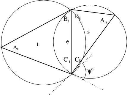
Formula 3.1

$$\psi^{e}=\psi^{e}_{s}+\psi^{e}_{t}$$

with

$$\psi^{e}_{\tau}=\frac{B_{\tau}+C_{\tau}-A_{\tau}}{2}$$

using the notation in the first figure.

Comment on Proof: This formula always holds on a constant curvature surface, and a proof can be found in [8]. For our purposes it is useful to introduce the key object showing up in the proof of the negative curvature case. This object is an ideal hyperbolic prism. The prism is constructed from the angle data of a hyperbolic triangle, namely a set of positive angles $\{A,B,C\}$ such that $A+B+C-\pi<0$. To construct it first form a hyperbolic triangle with the $\{A,B,C\}$ data, then place the triangle on a hyperbolic plane and then place the plane in hyperbolic three space. Now union this triangle with the geodesics perpendicular to this 2-plane going through the vertices of the triangle. The prism of interest is the convex hull of this arrangement. See Figure 2.

Figure 2: The prism.

Now suppose we have any triangulation of a Riemannian surface with varying curvature; What data may we collect? Well, we may collect the topological triangulation ${\bf T}$ and all the triangle angles. From formula 3.1 this triangle angle data may be organized into the collection of partial angles $\psi^{e}_{t}$, whose values we will identify with the coordinates in a $3F$ dimensional real vector. It should be pointed out that the angles inside the triangles are linearly determined by the $\psi^{e}_{t}$ via inverting formula 3.1. To be the data of a Delaunay triangulation forces certain natural linear constraints, which we will capture with the following definition.

Definition 3.2

Let an angle sytem be any point $x$ in the above vector space such that $x$’s associated triangle angles are in $(0,\pi)$ and sum up to $2\pi$ at any vertex. A Delaunay angle system is an angle system $x$ where the complement of the informal intersection angle, $\psi^{e}(x)=\psi^{e}_{s}(x)+\psi^{e}_{t}(x)$, has values in $(0,\pi)$.

We call two angle systems $x$ and $y$ conformally equivalent if they share the same informal intersection angles. We record this with idea the following definition.

Definition 3.3

$x$ and $y$ will be called conformally equivalent if $\psi^{e}(x)=\psi^{e}(y)$ for all $e$.

Motivated by the Gauss-Bonnet formula we also define the following.

Definition 3.4

The curvature of a triangle $t$ relative to an angle system $x$ is defined to be $\pi$ subtracted from sum of the triangle angles in $t$ determined by $x$. If every triangle has negative curvature relative to $x$, then $x$ will be said to have negative curvature. The set of Delaunay angle systems with negative curvature will be denoted ${\bf N}_{x}$.

There is a simple set of linear equations which will gaurentee that a Delaunay angle system is conformally equivalent an angle system in ${\bf N}_{x}$. Let $S$ be a set of triangles in ${\bf T}$, and denote the cardinality of $S$ as $|S|$.

Definition 3.5

An angle system $x$ will be called teleportable if for any set of triangles $S$ we have

$$\sum_{e\in S}(\pi-\psi^{e}(x))>\pi|S|.$$

As an immediate consequence of theorem 2 in [8] we have the following lemma.

Lemma 3.6 (The Discrete Teleportation Lemma)

A Delaunay angle system $x$ is teleportable if and only if $x$ is conformally equivalent to a negative curvature Delaunay angle system.

The proof of this lemma is completely linear in nature.

In the setting here we will only be concerned with Delaunay angle systems satisfying the conditions of this lemma, which includes the angle data associated to a Delaunay triangulation of surface with varying negative curvature.

The pleasure derived from the Delaunay angle systems comes from a wondrous objective function which lives on ${\bf N}_{x}$. Let $V_{t}(x)$ denote the volume of the ideal hyperbolic prism constructed from a triangle $t$’s angle data relative to $x$, as described in the previous section. Now simply let the objective function be

$$H(x)=\sum_{t\in{\bf T}}V_{t}(x).$$

The wonder of this function can best be felt by examining its differential. To compute this use $x$’s angle data in $t$ to construct a hyperbolic triangle and let $l^{e}_{t}(x)$ denote the length of the edge $e$ in this triangle. In [8] the following formula is produced:

Formula 3.7

$$dH=-\sum_{(e,t)}\log\left(\frac{\cosh(l^{e}_{t}(x))-1}{2}\right)d\psi_{t}^{e}$$

The tangent space at any point of ${\bf N}_{x}$ is precisely the set of directions preserving the condition that the $\psi^{e}$ are constant, hence is spanned by vectors in the form $C^{e}=\frac{\partial}{\partial\psi^{e}_{t}}-\frac{\partial}{\partial\psi^{e}_{s}}$. So from formula 3.7 we see that $x$ is a critical point of the objective function in a conformal class if and only if

$$0=dH(C^{e})=\log\left(\frac{\cosh(l^{e}_{t}(x))-1}{2}\right)-\log\left(\frac{\cosh(l^{e}_{s})-1}{2}\right)$$

for all edges $e$. Thus at a critical point of $H$ we have that $l^{e}_{t}(x)=l^{e}_{s}(x)$, so the set of hyperbolic triangles formed from $x$’s angle data fit together to form an actual hyperbolic surface.

Definition 3.8

A Delaunay angle system which is the angle data of a hyperbolic surface will be called uniform.

The question becomes: how many (if any) uniform structures can be associated to a given angle system? The objective function can be analyzed and using a compactness argument with boundary control, we find this objective function always achieves its maximum (see [8]). $H$ is also observed to be strictly concave down, so in fact any critical point is $H$’s unique maximum, and we have

Theorem 3.9 (The Discrete Uniformization Theorem)

If $\chi(M)<0$ and $x$ is a teleportable Delaunay angle system, then $x$ is conformally equivalent to a unique uniform angle system.

Remark 3.10

At this point it may be unclear how the above discussion is related to a disk pattern problem. Given a geodesic triangulation of a hyperbolic surface, the disk pattern of interest here is the disk pattern produced by the circumscribing disks of the triangulation’s triangles, which we will call the “empty pattern”. Notice in the presence of the “empty pattern” we may assign to each edge the value of the intersection angle between the circumscribing disks of the triangles sharing this edge. A pattern production theorem in this setting is an assurance of the existence of an “empty pattern” given a topological triangulation and the specification of a sensible intersection angle to each edge. To discover what sensible means it is necessary to strengthen lemma 3.6 to

Lemma 3.11

Given any topological triangulation and set of data $\psi^{e}\in(0,\pi)$ satisfying both $\sum_{e\in v}\psi^{e}=2\pi$ and the teleportability condition, there is $y\in{\bf N}_{x}$ satisfying $\psi^{e}(y)=\psi^{e}$.

Hence from theorem 3.9, under these hypothesis there is an “empty pattern” with intersection angles given by $\pi-\psi^{e}$, and we have solved our disk pattern problem.

This pattern problem is equivalent to a generalization of the convex ideal case of the Thurston-Andreev theorem when $\chi(M)<0$ (see [8] for the details and various generalizations). In the Euclidean case, this extension was carried out by Bowditch in [1], using techniques similar to Thurston’s original techniques found in [14]. The use of an objective function for solving such problems was introduced in Colin de Verdière’s [3] (see Question 5.1), while the use of hyperbolic volume as an objective function for producing disk patterns has its origin in Brägger’s beautiful paper [2]. Hyperbolic volume is also used as an objective function in Rivin’s [12].

4 Continuous Conformal Uniformization

The goal now is to bootstrap from the discrete uniformization procedure in the previous section to a procedure for producing a conformally equivalent uniform metric on a Riemannian surface. Two metrics on $M$, $g$ and $h$, are conformally equivalent if $h=e^{2\phi}g$ for a smooth function $\phi$. For metrics by uniform structure I will mean a metric with constant curvature. Our goal is to prove the classical result…

Theorem 4.1 (The Metric Uniformization Theorem)

Every metric is conformally equivalent to a metric of constant curvature, and this metric is unique up to scaling.

We will always be thinking in terms of a fixed background metric called $g$ and will label its associated geometric objects like its gradient, Laplacian, curvature, norm, area element, or area as $\nabla$, $\Delta$, $k$,$|\cdot|$ , $dA$ or $A$. For the $h=e^{2\phi}g$ metric we shall denote these objects with an $h$ subscript.

For starters let us note in the metric world we still have

Lemma 4.2 (The Metric Teleportation Lemma)

Every metric on a surface is conformally equivalent to a metric with either negative, positive, or zero curvature.

As in the discrete case, this part of the uniformization procedure is completely linear and follows at once from the facts that $k_{h}=e^{-2\phi}(-\Delta\phi+k)$ and that $C^{\infty}(M)$ is the $L^{2}$ orthogonal direct sum of $\Delta(C^{\infty}(M))$ and the constant functions. With this observation in mind, in our $\chi(M)<0$ world we will restrict our attention to metrics with strictly negative curvature, and from here on out we will assume $h$ has negative curvature everywhere.

As described in section 2, relative to a fixed set of vertices we may apply Delaunay’s “empty sphere” method and produce both the Delaunay triangulation and its associated “empty disk pattern” (see remark 3.10). A conformal transformation of a metric preserves infinitesimal circles and the angles between them, hence for a dense enough set of vertices a conformal transformation of a metric nearly preserves the data in the “empty disk pattern”. In particular, when we conformally change our metric the angles in the associated Delaunay triangulation will change in a manner strongly resembling a discrete conformal change, as introduced in the previous section. With this observation in mind, if we choose a dense ${\bf p}=\{p_{1},\dots,p_{n}\}$ and a topological triangulation, $\bf{T}$, with ${\bf p}$ as its vertices, then we could measure how close to uniform $h$ is with the objective function of the previous section. Specifically, we could let

$${\bf H}_{h}({\bf p})=\sum_{t\in{\bf T}}V^{h}_{t}({\bf p}),$$

where $V^{h}_{t}({\bf p})$ is computed using the angle data associated to the triangulation viewed in the $h$ metric. This of course means connecting the needed vertices of ${\bf p}$ with $h$ geodesics and measuring the resulting $h$ angles.

To capture this dense enough set of vertices it is natural to average ${\bf H}_{h}$ over all sets of vertices with a fixed density and take the limit as the vertex density goes to infinity, as we did for the random variable $F$ in section 2. To be explicit, we will distribute points with a density $\lambda$ relative to $g$’s area measure, and replace the $R_{t}$ in remark 2.8 with the function that is $V_{t}^{h}$ if the “triple’s” disk (in $g$’s metric) is empty of points, and zero otherwise. We will denote the expected value as ${\bf E}^{g}_{\lambda}({\bf H}_{h})$, with the superscript $g$ there to remind us of the background metric choice. Let

$$I^{g}(h)=\lim_{\lambda\rightarrow\infty}{\bf E}^{g}_{\lambda}({\bf H}_{h}-{\bf H}_{g}),$$

where the second term, ${\bf H}_{g}$, is independent of $h$ and is needed only to normalize the computation. From this construction we expect that $I^{g}$ is an objective function capable of uniformizing a negatively curved metric, and to confirm this, it is useful to explicitly compute $I^{g}$.

Theorem 4.3

If $g$ and $h$ are conformally equivalent with $h=e^{2\phi}g$ then

$$I^{g}(h)=-\int_{M}|\nabla\phi|^{2}+(\Delta\phi-k)\log(\Delta\phi-k)+k\log|k|dA.$$

Proof: In performing this computation, we first easily arrive at the analog of formula 1, namely

$$I^{g}(h)=\frac{1}{6}\int_{V_{\delta}}(V^{h}(A_{1},A_{2},A_{3})-V^{g}(A_{1},A_{2},A_{3}))e^{-\lambda a(y)}(\lambda dA)^{3},$$ (4)

with $V^{h}(A_{1}^{h},A_{2}^{h},A_{3}^{h})$ the volume of the prism determined by the triangle angles $\{A^{h}_{1},A^{h}_{2},A^{h}_{3}\}$ formed using the $h$ metric. At this point theorem 4.3 follows from equation 4 exactly as equation 3 followed from equation 1: We change coordinates, Taylor expand, integrate, and use the mean value theorem, to arrive at our formula for $I^{g}(h)$ plus an error term which in this case is of the form $O\left(\lambda^{-\frac{1}{2}}\log(\lambda)\right)$. It should be noted that this procedure, which is straightforward when used to produce equation 3, becomes considerably more involved in this setting. First one must Taylor expand $A^{h}_{i}(r,\vec{\theta},p)$ in $r$, which involves solving the boundary value problem determined by the geodesic equation up to the second order. With this one may expand $V^{h}$ in $r$, though care is needed since $V^{h}$’s differential has singularities. The singularities can be dealt with, and the needed integrals explicitly computed, to arrive at theorem 4.3. The details can be found in [9]. ∎

Now we will use $I^{g}$ to mimic the proof of the discrete uniformization theorem form the previous section here in the metric world.

Proof of Theorem 4.1 First we confirm that critical points are uniform by computing $I^{g}$’s differential. Using the notation of theorem 4.3, it is natural to view $I^{g}$ as a function on the possible $\phi$ where $h=e^{2\phi}g$. With this view point we have that the Fréchet derivative of $I^{g}$ at $\phi$ in the direction $\psi$ is

$$DI^{g}(\psi)=-\int_{M}\Delta\psi\log|k_{h}|dA.$$ (5)

Comment. Equation 5 implies that the flow generated by $I^{g}$ is the “log Ricci” flow, and an alternate proof of theorem 4.1 is to use this use this flow as Hamilton used the Ricci flow in [6].

Back to our optimization proof. A straightforward regularity argument along with equation 5 for the Fréchet derivative assures us that $k_{{h}}$ is smooth at a critical point. From formula 5 at a critical point $\log|k_{h}|$ is $L^{2}$ orthogonal to $\Delta(C^{\infty}(M))$. Recalling once again that $C^{\infty}(M)$ is the $L^{2}$ orthogonal direct sum of $\Delta(C^{\infty}(M))$ and the constant functions, we see that $\log|k_{h}|$ is indeed constant. So, in analogy to the discrete case, a metric is critical if and only if it is uniform.

Using a well chosen space of candidate metrics we find that a compactness argument with boundary control guarantees the existence of a critical point where $I^{g}$ achieves its maximum value. For example one could use the “$x\log^{+}(x)$” Orlicz-Sobolov closure (see [5]) of

$$V=\{\phi\in C^{\infty}\mid\int_{M}\phi dA=0\mbox{ and }-\Delta\phi+k<0\},$$

along with some basic functional analysis to arrive at the needed existence statement (see [9] for the details).

Since $H_{g}$ was constructed out of scale invariant angle data, we can only hope for uniqueness up to scaling. As in the discrete case, the uniqueness follows from the concavity of $I^{g}$. To be more specific, we use the fact that all critical points are smooth and that the Fréchet Hessian at $\phi\in V$ applied to $(\psi,\psi)$,

$$D^{2}{\bf}I^{g}(\psi,\psi)=-\int_{M}|\nabla\psi|^{2}+\frac{(\Delta\psi)^{2}}{\Delta\phi-k}dA,$$ (6)

is strictly negative at a non-zero $\psi$ satisfying $\int_{M}\psi dA=0$.

So we have proved theorem 4.1 by mimicking the discrete case’s arguments. ∎

Notice that we appear to have an infinite number of objective functions, one for each metric $g$. Fortunately any pair of these objective functions differ only by a constant. In order to see this it is useful to recall two other functions related to metric uniformization, the $\log(\det(\Delta_{h}))$ and the metric entropy. The $\log$ of the determinant of the Laplacian had its uniformization properties explored by Osgood, Phillips, and Sarnak in [11], while the entropy

$$E(h)=-\int_{M}k_{h}\log|h_{h}|dA_{h}$$

turned up Hamilton’s paper on surface uniformization [6]. As a straightforward consequence of theorem 4.3 and Polyakov’s formula (see [10]) telling us that the $\log(\det(\Delta_{h}))$ with in a conformal class can be expressed as

$$\log(\Delta_{h})=-\frac{1}{6\pi}\left(\frac{1}{2}\int_{M}||\nabla\phi||^{2}dA+\int_{M}k\phi dA+\ln(A_{h})\right)+C(g),$$

we have

Corollary 4.4

Let $g$ and $h$ be conformally equivalent and let

$$M(h)=E(h)-12\pi\log\left(\frac{\det(\Delta_{h})}{A_{h}}\right).$$

Then $I^{g}(h)=M(h)-M(g)$.

So up to a constant our objective function is given by $M(h)$.

5 Questions

Question 5.1

In [3], Colin de Verdière suggested that objective functions related to circle pattern problems might be related to the determinant of the Laplacian. One certainly would hope for a more direct relationship than that provided by corollary 4.4, raising the following natural question: Is there a disk pattern objective function, ${\bf D}_{h}$, with the property that ${\bf E}^{g}_{\lambda}({\bf D}_{h})$ limits to $\log(\det(\Delta_{h}))$ when suitably normalized?

Question 5.2

Corollary 4.4 also reveals some unexpected properties of $I^{g}$. For example, there was no reason to expect that the roles of the $g$ and $h$ metric could be decoupled via $I^{g}(h)=M(h)-M(g)$; or even the mysterious implication that $I^{g}(h)=-I^{h}(g)$. Furthermore corollary 4.4 allows us to extend this objective function consistently to the space of all negatively curved metrics. Notice that $I^{g}(h)$ can be computed and discretely interpreted when $g$ and $h$ are not in the same conformal class. With this observation we are left with the following natural question: Does corollary 4.4 hold among all metrics with negative curvature? Notice in particular this would provide a local formula for the $\log(\det(\Delta_{h}))$ outside a conformal class.

Question 5.3

The idea of using disk patterns to explore uniformization can be traced back to Thurston [15]. Thurston’s original idea was to approximate the Riemann mapping with a disk pattern solution. Thurston’s idea was initially justified in [13] and has been developed considerably since then, see for example [7]. It would be interesting to implement the spirit of this approximation approach in this setting. For example it would be nice to answer the following question: If one takes a “dense” set of points on a Riemannian surface and forms the ”empty disk pattern”, can one measure in a meaningful way how far the uniform surface produced by theorem 3.9 is from the conformally equivalent uniform structure produced by theorem 4.1?

Question 5.4

This whole story carries over to the spherical case, with the exception of the convexity of the analogs of the objective functions $H$ and $I^{g}$. Can one use these same techniques to prove the corresponding uniformization results, even without convexity?

Question 5.5

Can techniques like these be applied to find geometric structures on 3-manifolds?

References

- [1] B. H. Bowditch. Singular euclidean structures on surfaces. J. London Math. Soc. (2), 44:553–565, 1991.
- [2] W. Brägger. Kreispackungen und triangulation. Ens. Math, 38:201–217, 1992.
- [3] Y. Colin de Verdiére. Un principe variationnel pour les empilements de cercles. Prépublication de l’Institut Fourier, Grenoble, 147:0–16, 1990.
- [4] B. Delaunay [Delone]. Sur la spheŕe vide. Proc. Internal. Congr. Mth., 1:695–700, 1928.
- [5] T. Donaldson. Non-linear elliptic boundary problems in orlicz–sobolov spaces. J. Diff. Eq., 10:507–528, 1971.
- [6] R.S. Hamilton. The ricci flow on surfaces. Contemporary Math., 71:237–262, 1988.
- [7] Z. He and O. Schramm. The -convergence of hexagonal disk packings to the riemann map. Acta Math., 180:219–245, 1998.
- [8] G. Leibon. Singular hyperbolic structures on a surface. In Preparation.
- [9] Gregory Leibon. Random Delaunay Triangulations, the Thurston-Andreev Theorem and Metric Uniformization. PhD thesis, UCSD, 1999.
- [10] A. Polyakov. Quantum geometry of bosonic strings. Phys. Lett. B, 103:207–210, 1981.
- [11] B. Osgood R. Phillips and P.Sarnak. Extremals of determinants of laplacians. J. Fun. Anal, 80:148–211, 1988.
- [12] I. Rivin. Euclidean structures on simplicial surfaces and hyperbolic volume. Ann. of Math (2), 139:553–580, 1994.
- [13] B. Rodin and D. Sullivan. The convergence of circle packings to the riemann mapping. J. Differential Geom., 26:349–360, 1987.
- [14] William P. Thurston. Three-Dimensional Geometry and Topology. The Geometry Center, University of Minnesota, draft edition, 1991.
- [15] W.P. Thurston. The finite riemann mapping theorem. Unpublished talk given at the International Symposium in Celebration of the proof of the Bieberbach Conjecture (Purdue University, 1985).