Compact lattice $U(1)$ and Seiberg-Witten duality:
a quantitative comparison

Abstract

It was conjectured some time ago that an effective description of the Coulomb-confinement transition in compact $U(1)$ lattice gauge field theory could be described by scalar QED obtained by soft breaking of the $N=2$ Seiberg-Witten model down to $N=0$ in the strong coupling region where monopoles are light. In two previous works this idea was presented at a qualitative level. In this work we analyze in detail the conjecture and obtain encouraging quantitative agreement with the numerical determination of the monopole mass and the dual photon mass in the vicinity of the Coulomb to confining phase transition.

UB-ECM-PF-04/10

April 2004

The $U(1)$ lattice gauge theory in four dimensions has been long studied [1]. Among other interesting features it is the simplest theory posessing a confining phase in four dimensions. This phase is separated from the Coulomb one by a phase transition that it is believed to be driven my monopole condensation. The order of such transition has been subject to debate for a long time.

The analysis of this phase transition are usually done with an extended Wilson action [2]

$$S=-\sum_{P}(\beta\cos\theta_{P}+\gamma\cos 2\theta_{P})\hskip 20.00003pt\theta_{P}\in[0,2\pi).$$ (1)

It was generally believed that generic values of the coupling $\gamma$ lead to a Coulomb-confinement transition of first order, with larger values of the coupling $\gamma$ yielding stronger transitions.

With the possibility to study larger lattices and, accordingly, to explore larger correlation lengths, from a numerical point of view, some evidence for a second order nature of the transition were found [3, 4], at least for negative values of $\gamma$. The critical exponents and the spectrum were measured. The ligthest part of spectrum, according to the authors of [3, 4] consists in a $0^{+}$ and a $1^{+}$ gaugeballs that appear to scale differently ($\nu=0.49(7)$ and $0.35(3)$ for $\gamma=-0.2$, respectively). Other states seem to be compatible with being multiple particle states. All states considered are created by local or quasilocal operators so they presumably carry no magnetic charge. These measurements have been repeated recently with high precision in the work [5].

A quite different set of measurements was performed by the Pisa group [6]. They explicitly construct operators that create and annihilate monopoles. They are non-local in the original (electrical) variables. These authors also analyzed the spectrum and found the dependence of the monopole ($0^{+}$) and the dual photon ($1^{+}$) on the gauge coupling in the confined phase, determining some effective critical indices. For the monopole they find $\nu^{\ast}=0.29(2)$.

Indeed it seems to be now universally accepted, that the phase transition is actually of first order, albeit a very weak one [7, 8, 9]. This indicates that the critical exponents found in [3, 4] have to be taken as effective and that very close to the phase transition its first order nature should finally reveal.

Nevertheless, even if no true new fixed point is found, it is still very interesting to understand analytically this transition as it is driven by monopole condensation. This problem was addressed in two previous works [10, 11]. These authors follow a continuum treatment (that will be used in the present work too) and this is justified a posteriori because the transition exhibits a very large correlation length, extending over many lattice spacings and therefore the cut-off effects are small, of ${\cal O}(a/\xi)$ if $\xi$ is the correlation length. The Pisa group has indeed checked that some kind of universality exists by using scaling arguments. Using a continuum language makes everything simpler.

A priori it is not obvious how to write an effective field theory description of the monopole field and its interactions. It was proposed in [10, 11] to use as guiding principle the formulation of $N=2$ SYM by Seiberg and Witten [12], suitably adapted for this scenario; the idea was to use a pattern of symmetry breaking providing at low energies the spectrum observed on the lattice. It was found in [11] that the effective theory previously formulated in [10] can predict a phase diagram that qualitatively agrees with the one found in lattice simulations corresponding to a weakly first order transition.

In this work we aim to extend such agreement from the qualitative to the quantitative level. We reproduce the plot of the mass of the monopole field found in [6] and check that in the confining phase its pseudo critical exponent $\nu$ is Gaussian. We also determine the mass of the dual photon state, that we actually use to match some continuum parameters to the lattice values.

The key point (see [11]) is to properly understand the scale dependence of the low-energy effective theory. In its original formulation, derived by Seiberg and Witten, the effective action provides the right description at a scale $|a_{D}|$ in the dual variables ($a_{D}$ being the v.e.v. of the dual scalar field which is a component of the original $N=2$ vector multiplet). As already explained in [11] at the scale $|a_{D}|$ the couplings freeze i.e. they stop running; this allows to extract the theory at $\mu\sim 0$ from the one at $\mu\sim|a_{D}|$.

In order to describe a scenario with $U(1)$ gauge symmetry and no supersymmetry ($N=0$) in [10] a two step supersymmetry breaking was introduced using both the coupling to a spurion superfield that has a non-zero value for its $D$ component (a technique borrowed from [13]) and to a $N=1$ superfield. The addition of the hard $N=1$ breaking is absolutely crucial as it allows us to decouple the value of $a_{D}$ from the point in moduli space one has to choose to define the theory; this allows the monopole to become light far from the original region in the (unperturbed) moduli space where $a_{D}\sim 0$. In fact, the value for $|a_{D}|$ for which the monopole become massless turns out to be close to ${D}_{0}$, where $D_{0}$ is the $D$ component of the spurion field that breaks $N=2$ down to $N=0$. In spite of the hard nature of the $N=1$ breaking term, the dual version of the effective action can still be determined to some extent, and this is sufficient for our purposes. The analytic structure of the Kähler prepotential $\mathcal{F}$ is unchanged.

Thus even if at the scale ($\mu\sim|a_{D}|)$ the form of the effective potential is uniquely determined from the Seiberg and Witten construction, at lower energies (the ones relevant for the comparison with the lattice results if we suppose the lattice scale at $\mu=1$) there are corrections produced by quantum effects due to the breaking of supersymmetry. This is how the Coleman-Weinberg mechanism [14, 15] triggers a (weak) first order transition.

Before entering into the details of the calculation we review the frameset where we work. This will also allow us to introduce the notation we shall use in the subsequent. Starting from the $N=2$ SYM [12] and breaking all the supersymmetries down to $N=0$ [13, 10] one obtains an effective theory whose Lagrangian density is:

$$\mathcal{L} = -\frac{1}{4}F_{\mu\nu}F^{\mu\nu}+\frac{1}{2}\partial^{\mu}m\partial_{\mu}m+\frac{1}{2}\partial^{\mu}\theta\partial_{\mu}\theta$$ (2)

$$+g_{{}_{D}}m\partial_{\mu}\theta A^{\mu}+g_{{}_{D}}\theta\partial_{\mu}mA^{\mu}+\frac{1}{2}g_{D}^{2}A^{\mu}A_{\mu}m^{2}$$

$$-\frac{\lambda}{16}m^{4}-\frac{1}{2}M^{2}m^{2}+\mathcal{L}_{g.f.}$$

The field $A_{\mu}$ denotes the dual photon ($J^{P}=1^{+}$) and $m,\theta$ are the polar components of the complex monopole field ($J^{P}=0^{+}$). The scalar potential is given by the two last terms in (2). In the previous formulae only light fields have been retained. The full effective lagrangian contains in addition fields of masses $\mathcal{O}({D_{0}})$, but we have not written these since we are eventually interested in the energy range for $p^{2}$: $0\leq p^{2}\ll b_{01}D_{0}$, and in this range they decouple (see [11] for the full spectrum). Thus the above lagrangian provides a valid description only below the scale $\mu={D_{0}}\simeq a_{D}$. The couplings $b_{ij}$ are expressed in terms of the original prepotential

$$b_{ij}\equiv\frac{1}{4\pi}\text{{Im}}\ \tau_{ij}=\frac{1}{4\pi}\text{{Im}}\ \frac{\partial^{2}\mathcal{F}}{\partial a_{D}^{i}\partial a_{D}^{j}},$$ (3)

the index ‘1’ denoting the physical fields and ‘0’, the spurion [13]. An important parameter is the monopole ‘mass’ term. At the scale ${D_{0}}$

$$M^{2}\equiv-\frac{\alpha}{b_{11}}.$$ (4)

Here

$$\alpha=-\left(2|a_{D}|^{2}+b_{01}D_{0}\right)$$ (5)

On the other hand the mass of the dual photon is given by the formula familiar from the Higgs mechanism. At tree level, reading from (2), $M_{V}=g_{D}\langle m\rangle$, where $\langle m\rangle$ is the expectation value derived from the tree level effective potential.

Let us remark once more that the prepotential $\mathcal{F}$ is unchanged by the $N=1$ breaking [10]. All the previous results hold at the supersymmetry breaking scale ${D_{0}}\sim|a_{D}|$. At this scale supersymmetry implies

$$g_{D}=\frac{1}{\sqrt{b_{11}}},\hskip 20.00003pt\lambda=\frac{2}{b_{11}}$$ (6)

Next we have to run the effective potential from the scale $\mu={D_{0}}$ down to $\mu\sim 1$ to compare with the lattice results. This is done in perturbation theory at the one-loop approximation. The result is

$$V=\frac{\lambda}{16}m^{4}+\frac{M^{2}}{2}m^{2}+\frac{1}{64\pi^{2}}\left(\frac{\lambda m^{2}}{4}+M^{2}\right)^{2}\ln\left(\left(\frac{\lambda m^{2}}{4}+M^{2}\right)\frac{1}{\mu^{2}}-\frac{3}{2}\right)+$$

$$\frac{1}{64\pi^{2}}\left(\hskip 2.5pt\frac{3\lambda m^{2}}{4}+M^{2}\right)^{2}\ln\left(\left(\frac{3\lambda m^{2}}{4}+M^{2}\right)\frac{1}{\mu^{2}}-\frac{3}{2}\right)+\frac{3m^{4}g_{D}^{4}}{64\pi^{2}}\ln\left(\frac{g_{D}^{2}m^{2}}{\mu^{2}}-\frac{5}{6}\right).$$ (7)

We quote here the relevant beta functions [16]

$$\beta_{g}=\frac{g_{D}^{3}}{48\pi^{2}}$$ (8)

$$\beta_{\lambda}=\frac{5\lambda^{2}}{16\pi^{2}}-\frac{3\lambda g_{D}^{2}}{4\pi^{2}}+\frac{3g_{D}^{4}}{2\pi^{2}}$$ (9)

$$\gamma_{m}=-\frac{3g_{D}^{2}}{8\pi^{2}}$$ (10)

$$\gamma_{M}=-2+\frac{\lambda}{8\pi^{2}}-\frac{3g_{D}^{2}}{8\pi^{2}}$$ (11)

At first glance the lagrangian (2) looks like standard scalar electrodynamics but there are some important remarks to be made. First of all, it is not even obvious that scalar electrodynamics is the natural language to describe the Coulomb-confinement transition. The supersymmetric origin prescribes a well defined relation between $g_{D}$ and $\lambda$ at the scale $\mu={D_{0}}$ (6) that can be extended to any other scale by using the renormalization group equations via the above beta functions. Furthermore there is a dependence of the mass term $M^{2}$ on $g_{D}$ that is also dictated by supersymmetry, and this turns out to be absolutely crucial to provide a successful description (see below).

Likewise the dual photon mass algo gets renormalized when running down from $\mu=D_{0}$ to $\mu=1$

$$M_{V}=g_{D}\langle m\rangle+\delta M_{V}$$ (12)

Here $g_{D}$ is the (dual) gauge coupling at scale $\mu=1$, $\langle m\rangle$ is the v.e.v. derived from (7) and $\delta M_{V}$ is the one-loop correction. We do not present it here but it has been included in our analysis.

Let us have a closer look at the definition of $M^{2}$. From (5), using the results of [13], we have

$$M^{2}=\left(2|a_{D}|^{2}+\frac{\Re a_{D}}{4\pi}D_{0}\right)g_{D}^{2}+\Im aD_{0}$$ (13)

On the other hand as already explained in [11] $|a_{D}|$ is the parameter that drives the phase transition whereas $a$ is related to the point on the moduli space of the original Seiberg-Witten construction.

As shown in detail in [10] and in [11], the addition of the $N=1$ breaking allows the use of $|a_{D}|$ as a free parameter triggering the monopole condensation. In fact, the value of $|a_{D}|$ is chosen so as to reproduce the critical coupling in the lattice. The relation between $a$ and $a_{D}$ is not completely determined because it is modified by the hard breaking that the $N=1$ term brings about. The form of the relation is derived in [10] using the charges under $U(1)_{A}\times U(1)_{R}$ symmetry. The value of $|a_{D}|$ is assumed to be tuneable by adjusting the value of the dimensionful parameter in the $N=1$ hard breaking term (called $w$ in [11]). Likewise the same mechanism should also allow us to tune the value for $\Im a$ by using the imaginary part of the same hard breaking parameter $w$ [10, 11] . In other words, we trade the two degrees of freedom of the complex parameter $w$ by $|a_{D}|$ and $\Im a$. It should be clear to the reader that this is an assumption, though a very reasonable one.

Thus, for simplicity, we write the monopole mass parameter $M^{2}$ as

$$M^{2}=\alpha_{0}+Ag_{D}^{2}$$ (14)

where $\alpha_{0}$ and $A$ (instead of $a_{D}$ and $D_{0}$) are adjustable (real) parameters in our approach to be matched to the lattice action. This should be valid up to higher orders in $g_{D}$ that do not really affect the essence of the discussion.

Let us now make contact with the lattice results. We shall identify the $g_{D}$ coupling with $\beta$ introduced in (1): $g_{D}^{2}=\beta$. This is a reasonable assumption considering the standard lattice-to-continuum relation $\frac{1}{g^{2}}=\beta$ in conjuction with the relation between direct and dual couplings $g_{D}=1/g$ and the fact that in the continuum the gauge coupling is associated to a conserved current. The value of ${D_{0}}$, the supersymmetry breaking scale, as explained in detail in [11], can be thought as the ultraviolet cut off for the bare lagrangian (2).

The continuum model hence depends on 4 parameters: $g_{D},D_{0},\alpha_{0}$ and $A$. Our results depend very weakly on the value of $D_{0}$. This is due to the fact that the lattice phase transition (and the continuum version of it) is weakly first order so in the range of energies we are considering (where the physical observables obey a pseudo scaling and a finite size analysis produces the typical collapse of the data expected in a second order phase transition [6]) we expect a very weak dependence of our results on the UV cut-off $D_{0}$. This assumption has been checked by varying the value of $D_{0}$. We must however ensure the validity of the one loop approximation for the beta functions.

Given these assumptions we are left with an effective theory depending on one parameter ($g_{D}$) that is directly related to the lattice model and two free parameters $\alpha_{0},A$ that we should fix matching some physical observables between the lattice and the continuum results (actually the lattice can be thought of a continuum theory with an infinite number of higher dimensional operators too if we want to look at it in this way).

In the work of [6] two physical observables directly accessible in our model have been measured, namely $M_{V}^{latt}(\beta)$ and $M^{latt}(\beta)$: the dual photon and the monopole masses. The notation emphasizes that they are lattice results. The measurement is reasonable for the dual photon mass, but with enormous error bars for the monopole mass. On the other hand, $M_{V}(g_{D},\alpha_{0},A),M(g_{D},\alpha_{0},A)$ refer to the curves we obtain in the continuum theory for the masses as a function of the free parameters. In our model both of these curves can be easily calculated. Just to fix ideas, the parameters $g_{D},\alpha_{0}$ and $M$ have to be understood at the scale $D_{0}$. The renormalization group allows us to determine its value at the relevant scale $\mu\sim 1$ as well as the rest of the parameters that are related to them (such as $\lambda(\mu\sim 1)$)

The monopole condensate for instance $\langle m\rangle$ is obtained at the one loop level by minimizing the potential (7). The monopole mass $M^{2}(g_{D},\alpha_{0},A)$ is obtained as the second derivative of the potential (7) with respect to $m$ field at its minimum $m=\langle m\rangle$. We decided to use the dual photon mass to do the matching procedure due to the better numerical accuracy of these results in [6]. We fix the two parameters $\alpha_{0},A$ by requiring that at two points of the curve $M_{V}^{latt}(\beta)$ our results coincide with the lattice one. Since $g_{D}$ is assumed to correspond to $\sqrt{\beta}$ matching these two points determine $\alpha_{0}$ and $A$.

Let us now summarize the way we proceed

1.- The gauge coupling constant is matched to the lattice $g_{D}(\mu=1)\equiv\sqrt{\beta}$

2.- The renormalization group is used to run upwards to the scale where the effective potential derived from duality arguments is valid $g_{D}(\mu=1)\to R.G.E.\to g_{D}(\mu={D_{0}})$ and we require $\lambda(\mu={D_{0}})=2g_{D}^{2}(\mu={D_{0}})$

3.- We use the renormalization group to run downwards the scalar coupling $\lambda(\mu={D_{0}})\to R.G.E.\to\lambda(\mu=1)$ At this step we obtained the before mentioned relation between $\lambda$ and $g_{D}$ at the lattice scale.

4.- We fix the values of $\alpha_{0}(\mu={D_{0}})$ and $A(\mu=D_{0})$ so as to match the lattice curve for the dual photon mass at two points $\beta_{1},\beta_{2}$, in the sense $M_{v}^{latt}(\beta_{1})=M_{V}(\alpha_{0},A,\sqrt{\beta_{1}});\ \ M_{v}^{latt}(\beta_{2})=M_{V}(\alpha_{0},A,\sqrt{\beta_{2}})$. In our scenario the order parameter for the Coulomb to confined transition is $\langle m\rangle$. The appeareance of a non-trivial (i.e. away from the origin) minimum will signal the Higgs phase in the dual (continuum) model and the confined phase on the lattice.

We have to notice that even if not explicitly written, the field $m$ also runs down to $\mu=1$ as $m=m_{0}/\sqrt{Z_{m}(\mu)}$ . We take $Z_{m}({D_{0}})=1$.

Figure 1: The figure shows the lattice results for the mass of the dual photon $J^{P}=1^{+}$ (dots) and the monopole $J^{P}=0^{+}$ (squares) versus $\beta$ from [6] and their fit to the former assuming criticality (thin solid line). The thick lines correspond to the prediction from our model after the matching procedure discussed in the text. Two points of the curve $M_{V}(\beta)$ measured on the lattice are used to fix the free parameters in the model we are using. This allows to predict the critical exponent for $M_{V}(\beta)$ and the curve $M(\beta)$ describing the monopole mass. Clearly our model (with a weak first order transition) describes well the dual photon data and gives a very reasonable description of the monopole mass.

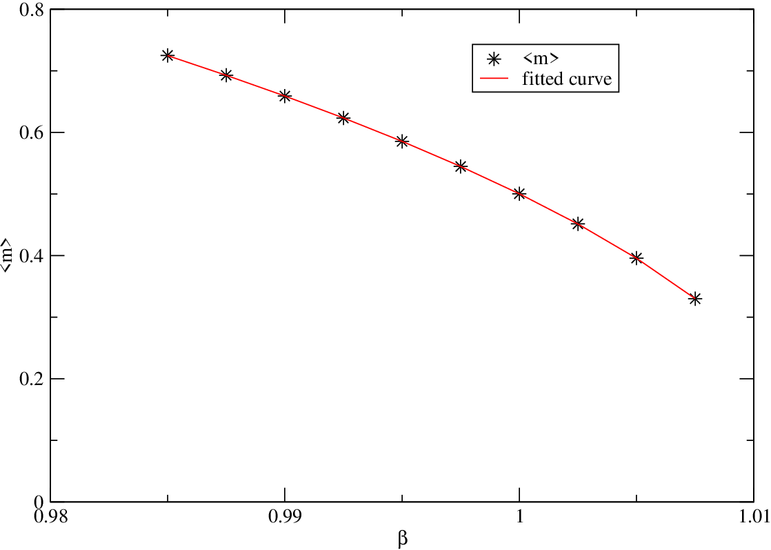
Doing this we are able to compare our results with the ones obtained in lattice simulations (shown in figure 1) and make predictions about the critical exponent of the curve of the dual photon mass as shown in figure 2: the pseudo-critical exponent emerging from our fit is $\nu^{\ast}\simeq 0.46(1)$.

After matching $\alpha_{0}$ and $A$ everything else is defined and we can now obtain the curve $M(g_{D})$ for the monopole mass as shown in fig. 3 and fig. 1. A value for the pseudo-critical exponent $\nu^{\ast}=0.49(1)$ is obtained. The uncertainty reflects the freedom in choosing $D_{0}$ and the numerical errors of the points we use to fix the parameters; we take $D_{0}$ in the range $10^{2}-10^{3}$ in lattice units. Larger values translate in inconsistencies of the one-loop RGE. Figure 4 shows the evolution of the monopole mass across the phase transition.

Figure 2: Dual photon mass versus $\beta$ and fit.

Figure 3: Monopole mass obtained from the continuum model versus $\beta$ and fit.

Figure 4: The figure shows the results we obtain for the monopole and the dual photon masses across the transition. Even if at the transition the masses seems to vanish they have a non zero value $\mathcal{O}(10^{-2})$ fingerprint of the first order nature of this transition. This small value compared with the other masses supports an effective theory approach of the transition and arises from its weak nature (fluctuation induced) .

The monopole condensate can also be obtained and it is plotted in fig.5. Extracting the pseudo-critical exponent we obtain $\delta^{\ast}\simeq 0.48(1)$. The results of [6] lead to $\delta^{\ast}=1.1\pm 0.2$. In figure 5(b) we show the results for the condensate obtained using the Villain action [17]. It is found in these simulations that the critical index is $\delta^{\ast}=0.197(3)$. Clearly there is a lot of room for improvement in the numerical simulation field., particularly in what concerns the monopole. Our prediction on the other hand is quite clear; the exponent for the condensate should also be Gaussian.

Our results and predictions are also questionable. Apart from the main conjecture about the form of the quantum corrections due to the $N=1$ breaking, that we regard as a mild one, we have derived our results using the one-loop effective potential and one-loop beta functions. Some conclusions are actually independent of this, for instance the existence of a first-order phase transition due to the Coleman-Weinberg phenomenon. But detailed numerics do of course depend on this approximation. The fact is that we are always in the weakly coupled phase so the results should be trustable with a typical ’perturbative’ error which indeed seems to be reasonably small.

Figure 5: Monopole condensate versus $\beta$ and fit and the analogue result obtained in [17]. The lattice results are obtained using the Villain action.

To conclude, the arguments based on duality provide a well defined form of the long-distance effective action, including a well prescribed form of the dependence of the mass parameted in $g_{D}$, the relation between the scalar coupling $\lambda$ constant and $g_{D}$ and so on. This form of the effective action seems to reproduce well the behaviour observed in lattice simulations. A clear prediction of our model is that the phase transition is of first order everywhere.

We have obtained a good qualitative agreement with the (still rather crude) results of the lattice simulations concerning mass of the dual photon, the monopole mass, the monopole condensate and its pseudocritical exponents.

We believe that our results show that the dual Higgs mechanism is at work in lattice $U(1)$.

A very interesting aspect is to understand the relation between the spectrum of the gaugeballs measured in the $U(1)$ lattice gauge theories [4, 5], and the spectrum of the dual abelian Higgs model we are considering. In [10] a correspondence based on the identification of the quantum number $J^{P}$ was proposed. While this argument for the gauge ball state $1^{+}$ might be correct, we think that it cannot safely be extended to the identification of the $0^{+}$ gaugeball with the monopole since the former carries no magnetic charge. The identification is thus questionable.

On the other end we would expect that a well defined effective theory must include all the light degrees of freedom appearing in the original model. So we expect that there should be an interpretation of the above gaugeball states in terms of monopole-antimonopole weakly bound states, but for the moment we cannot give a precise statement that fulfills our expectations. We think that this problem deserves further study.

We regard these explorations as being both interesting and urgent to enlarge our understanding of the mechanisms behind confinement.

References

- [1] M. Creutz, L. Jacobs and C. Rebbi, Phys. Rev. D 20 (1979) 1915.
- [2] G. Bhanot, Nucl. Phys. B 205 (1982) 168.
- [3] J. Jersak, C. B. Lang and T. Neuhaus, Phys. Rev. Lett. 77 (1996) 1933 [arXiv:hep-lat/9606010]. J. Cox, W. Franzki, J. Jersak, C. B. Lang, T. Neuhaus and P. Stephenson, Nucl. Phys. Proc. Suppl. 53 (1997) 696 [arXiv:hep-lat/9608106].
- [4] J. Cox, W. Franzki, J. Jersak, C. B. Lang, T. Neuhaus and P. W. Stephenson, Nucl. Phys. B 499 (1997) 371 [arXiv:hep-lat/9701005].
- [5] P. Majumdar, Y. Koma and M. Koma, Nucl. Phys. Proc. Suppl. 129-130 (2004) 811 [arXiv:hep-lat/0309038].
- [6] A. Di Giacomo and G. Paffuti, Phys. Rev. D 56 (1997) 6816 [arXiv:hep-lat/9707003].
- [7] I. Campos, A. Cruz and A. Tarancon, Nucl. Phys. Proc. Suppl. 73 (1999) 715 [arXiv:hep-lat/9808043]; Nucl. Phys. B 528 (1998) 325 [arXiv:hep-lat/9803007]; Phys. Lett. B 424 (1998) 328 [arXiv:hep-lat/9711045].
- [8] G. Arnold, B. Bunk, T. Lippert and K. Schilling, arXiv:hep-lat/0210010. Nucl. Phys. Proc. Suppl. 94 (2001) 651 [arXiv:hep-lat/0011058].
- [9] M. Vettorazzo and P. de Forcrand, Nucl. Phys. B 686 (2004) 85 [arXiv:hep-lat/0311006].
- [10] J. Ambjorn, N. Sasakura and D. Espriu, Fortsch. Phys. 47 (1999) 287; Mod. Phys. Lett. A 12 (1997) 2665 [arXiv:hep-th/9707095].
- [11] D. Espriu and L. Tagliacozzo, Phys. Lett. B 557 (2003) 125 [arXiv:hep-th/0301086].
- [12] N. Seiberg and E. Witten, Nucl. Phys. B 426 (1994) 19 [Erratum-ibid. B 430 (1994) 485] [arXiv:hep-th/9407087]; Nucl. Phys. B 431 (1994) 484 [arXiv:hep-th/9408099].
- [13] L. Alvarez-Gaume and M. Marino, arXiv:hep-th/9606168, Int. J. Mod. Phys. A 12 (1997) 975 [arXiv:hep-th/9606191]. L. Alvarez-Gaume, J. Distler, C. Kounnas and M. Marino, Int. J. Mod. Phys. A 11 (1996) 4745 [arXiv:hep-th/9604004].
- [14] S. R. Coleman and E. Weinberg, Phys. Rev. D 7 (1973) 1888.
- [15] H. Yamagishi, Phys. Rev. D 23 (1981) 1880.
- [16] M. A. Ahmed, Phys. Rev. D 11 (1975) 2136.
- [17] J. Jersak, T. Neuhaus and H. Pfeiffer, Phys. Rev. D 60 (1999) 054502 [arXiv:hep-lat/9903034].