From Triangular Array Progression
to Near-Log-Concave State Transitions

Abstract

The paper introduces an infinite integer sequence progression that produces a triangular array for which the $n$th row sums to $2^{n}$ for every $n\geq 0$. Every row of the triangular array can be realized as the degree sequence of a multigraph without loops. Although the first four rows coincide with those from Pascal’s triangle, the proposed array progression becomes asymmetric and diverges from binomial coefficients thereafter. The triangular array hosts infinitely many unimodal near-log-concave sequences with no zeros, and its log-concavity deviation converges to $\log(4/3)$ under logarithmic scaling. The progression provides a probability measure at every generation, defines what we call near-log-concave random variables, produces state-transitions of an infinite Markov chain, and hosts a totally-positive Toeplitz matrix of order two. We study the Shannon entropy dynamics of the construct, and present an application in physics to model systems exhibiting a set of state-transition characteristics that govern jumps of electrons across different energy states. We provide a transformation of the triangular array over the Tychonoff cube to produce an infinite family of right-stochastic matrices, all satisfying the given set of state-transition characteristics.

Keywords: Triangular array, unimodal sequence, log-concavity, multigraph, stochastic matrix

1 Introduction

The main direction of this paper is to introduce and study an infinite triangular array generated through a particular sequence progression algorithm. We shall keep this paper reasonably compact, and provide analytical and numerical results that shed light on how the proposed construct behaves. As a brief background to its emergence, the author uncovered the triangular array sequence while working on a probability problem involving systems that satisfy the following set of state-transition characteristics:

1. From any state, the system has the highest probability to remain in that state in the next time step when compared to any other one state

2. From any state, transition probabilities are monotonically non-increasing from the closest previously-visited state to progressively distant previously-visited states in the next time step

3. From any state, the system can transition only to the closest unvisited state in the next time step

As an overview, such a stochastic system has the highest likelihood to stay where it currently is when compared to transitioning to another state. If this system transitions to another previously achieved state, the transitioned state is more likely to neighbor the current state than to being further away from it. Finally, the system visits only the closest new state and no other previously unexplored state is achieved in one time step. Such dynamical systems, either partially or fully, may be observed in atomic phase transitions, social queuing, cellular cycles and gene expressions – see [4, 13, 17, 18, 20, 22, 28, 33] and references therein. For example, in quantum mechanics and atomic physics, such patterns may arise in systems wherein electrons jumping to lower energy states (i.e. more ordered states) is more probable than leaping to a higher energy state (i.e. a more disordered state); e.g. quantum random walks may exhibit similar left-skewed, asymmetric behaviour (see [15, 27]). We shall later present numerical simulations for systems with such characteristics based on the proposed triangular array. Furthermore, we shall provide a method to transform the given triangular array, which we use as an anchor integer structure, into infinitely many transition matrices that satisfy all the three aforementioned characteristics, providing infinitely many candidates to model such systems. To the best of our knowledge, the construct presented in this paper does not exist in the literature.

We show that the introduced anchor integer triangular array hosts infinitely many unimodal near-log-concave sequences with no zeros. In doing so, we first prove that there exists an infinite sub-triangular array, – each row a strictly-positive log-concave sequence (i.e. a Pólya frequency sequence of order 2) – that almost entirely dominates the full triangular array, in which log-concavity fails only at a single early column. At this stage, we shall highlight that log-concave sequences arise in numerous areas of mathematics including algebraic graph theory, combinatorics and geometry – see [7, 10, 11, 14, 16, 19, 23, 26, 30, 31, 35, 36, 37], amongst many other important works. Next, we prove that every row of the triangular array sums to an increasing power of 2, where the power is determined in terms of the cardinality of that row; more precisely, the $n$th row of the array sums to $2^{n}$ for every $n\geq 0$. We show that every row of the array defines the degree sequence of a multigraph without loops; see [6]. Although the first four rows of the proposed triangular progression coincide with those from Pascal’s triangle, its elements become asymmetric thereafter and diverge from binomial coefficients. Accordingly, when viewed as polynomial coefficients, the proposed triangular array produces a family of polynomials that diverge from $(x+1)^{n}$ for $n\geq 4$. We show that the divergence polynomial must have a root at 1 for every $n\geq 0$. In addition, we define a log-concavity deviation measure in order to quantify how far a near-log-concave sequence is to being log-concave. We prove that the log-concavity deviation of the triangular progression converges to $\log(4/3)$ under logarithmic scaling.

In addition, due to the positivity of every element in the triangular progression, we achieve infinitely many probability mass functions by normalising the integer triangular array by an increasing power of 1/2. Accordingly, the construct forms a lower-triangular stochastic matrix of a Markov chain with infinite states. Moreover, we show that such a Markov chain with the proposed stochastic matrix satisfies the three state-transition characteristics as mentioned above. We also prove that the normalised array hosts an infinite Toeplitz matrix that is totally-positive of order 2 with each row log-concave. Since every probability mass function extracted from the structure is near-log-concave, we define what we call near-log-concave random variables and their induced probability measures. Here, we highlight that log-concavity arises abundantly in probability and statistics; e.g. Gaussian, Bernoulli, Poisson, exponential and geometric distributions are log-concave distributions – see [3, 8, 9, 24, 25, 32, 38] and references therein. Next, we study the Shannon entropy dynamics – see [2, 5, 12, 21, 29] – of the normalised triangular array progression to quantify the evolution of information from one row to the next.

For purposes strictly surrounding the aforementioned state-transition characteristics, having near-log-concavity is not a necessary condition, but it leads us to prove unimodality, which is necessary (but not sufficient). More precisely, a sequence $[\eta_{1},\ldots,\eta_{n+1}]$ for $n\geq 1$ is unimodal if there exists a $k^{*}\leq n+1$ such that

$$\eta_{1}\leq\eta_{2}\ldots\leq\eta_{k^{*}}\,\,\,\,\,\text{and}\,\,\,\,\,\eta_{k^{*}}\geq\ldots\geq\eta_{n+1}.$$ (1)

If each row of a stochastic matrix satisfies (1) at $k^{*}=n$ for any $n\geq 1$, then the first two state-transition characteristics are satisfied – this will be clear later in the paper, where we show that each row of the normalised array progression satisfies this property.

2 Triangular Array Progression

Let $\mathcal{T}_{n,j}$ be the $n$th row and the $j$th column of the triangular array $\mathcal{T}$ for every $n\geq 0$ and $1\leq j\leq n+1$, given that $n,j\in\mathbb{Z}_{+}$. Our focus on triangular constructs stems from the third state-transition property mentioned in the previous section – from any state, the system can transition only to the closest unvisited state in the next time step – for which, a lower-triangular structure naturally embeds this characteristic when normalised into a stochastic-matrix, and when the upper-triangular cut is assumed to be all zeros. In order to capture the first and second state-transition properties given in the previous section, we ask additional properties from the infinite triangular array $\mathcal{T}$. For what follows, let $M^{*}\in\mathbb{Z}_{+}$ with $0<M^{*}<\infty$ be such that all rows $n\leq M^{*}$ of $\mathcal{T}$ are initialized and there exists no other initialization of $\mathcal{T}$ for any row $n>M^{*}$. Hereafter, every initialized row of $\mathcal{T}$ should be understood to satisfy all the three state-transition properties given in the previous section under a given normalization. Accordingly, for every row $n>M^{*}$, we shall first propose the following general array progression algorithm, which will later produce the special tringular array we will focus on.

General Construct of $\mathcal{T}$ after $M^{*}$:

1. $\mathcal{T}_{n,n+1}=F(\mathcal{T}_{k,k+1}\,:\,0\leq k\leq n-1)$ for every $n>M^{*}$

2. $\mathcal{T}_{n,n}=G(\mathcal{T}_{k,k}\,:\,0\leq k\leq n-1)$ for every $n>M^{*}$

3. $\mathcal{T}_{n,j}=H^{(j)}(\mathcal{T}_{k,j}\,:\,0\leq k\leq n-1)$ for every $1\leq j\leq n-1$ and $n>M^{*}$

given that $F,G$ and $H^{(j)}$ for $j\geq 1$ are $\mathbb{R}_{+}$-valued functionals on sequences that satisfy the following relations:

1. $G(\mathcal{T}_{k,k}\,:\,0\leq k\leq n-1)\geq F(\mathcal{T}_{k,k+1}\,:\,0\leq k\leq n-1)$ for every $n>M^{*}$

2. $G(\mathcal{T}_{k,k}\,:\,0\leq k\leq n-1)\geq H^{(n-1)}(\mathcal{T}_{k,n-1}\,:\,0\leq k\leq n-1)$ for every $n>M^{*}$

3. $H^{(j)}(\mathcal{T}_{k,j}\,:\,0\leq k\leq n-1)\geq H^{(j-1)}(\mathcal{T}_{k,j}\,:\,0\leq k\leq n-1)$ for every $2\leq j\leq n-1$ and $n>M^{*}$

Although the construct of $\mathcal{T}$ given above is fairly abstract for specific applications, it provides a mathematical structure that encapsulates all the three state-transition properties we aim to capture. More precisely, the functional relations above produce unimodal sequences where the mode manifests at the $n$th column of the $n$th row until which the sequence is monotonically non-decreasing. In addition, the $(n+1)$th column is at most as high as the $n$th column, and the triangular structure confines any view beyond column $n+1$. For the rest of this paper, we shall introduce and focus on an explicit construct of $\mathcal{T}$ that can be viewed as a particular example of the progression given above. Accordingly, $\mathcal{T}$ that forms our anchor integer structure is produced through the following special sequence progression algorithm:

1. $\mathcal{T}_{n,n+1}=1$ for every $n\geq 0$

2. $\mathcal{T}_{2,2}$ = 2 and $\mathcal{T}_{3,3}=3$

3. $\mathcal{T}_{n,n}=\sum_{k=1}^{n-2}\mathcal{T}_{n-k,n-k}$ for every $n\geq 4$

4. $\mathcal{T}_{n,j}=\mathcal{T}_{n-1,j}+\psi(j)$ for every $n\geq 1$ and $1\leq j\leq n-1$

given that $\psi:\mathbb{N}_{+}\setminus\{0\}\rightarrow\mathbb{N}_{+}$, where $\psi(1)=0$, $\psi(2)=1$, $\psi(3)=2$ and

$$\psi(j)=\sum_{k=1}^{j-1}\psi(k)\hskip 7.22743pt\text{for $j\geq 4$}.$$ (2)

Remark 2.1.

The explicit construct of $\mathcal{T}$ above is an example of the general construct when one sets $M^{*}=3$ and initialize every row $n\leq 3$ in agreement with the explicit algorithm.

Using the initial values $\psi(1)=0$, $\psi(2)=1$, $\psi(3)=2$ and the initial values $\mathcal{T}_{2,2}$ = 2 and $\mathcal{T}_{3,3}=3$, we have the following boundary relation, which we shall use later on:

$$\mathcal{T}_{n-1,j}+\psi(j)<2\mathcal{T}_{n-1,j}\,\,\Rightarrow\,\,\frac{\mathcal{T}_{n,j}}{\mathcal{T}_{n-1,j}}<2,$$ (3)

for every $n\geq 1$ and $1\leq j\leq n-1$, since $x+c<2x$ for any $c<x$ for $x,c\in\mathbb{R}_{+}$. Hereafter, we denote $\mathcal{T}_{n,*}$ as the full sequence of numbers at the $nth$ row of $\mathcal{T}$, given by

$$\mathcal{T}_{n,*}\triangleq[\mathcal{T}_{n,1}\,,\,\ldots\,,\,\mathcal{T}_{n,n+1}],$$

for every $n\geq 0$, where $[\,.\,]$ is the notation we use for any sequence – in this paper, any $[\,.\,]$ is composed of $\mathbb{R}$-valued elements and any infinite sequence should be understood asymptotically. Note that $\mathcal{T}_{n,*}$ for $n\in\{0,1,2,3\}$ are symmetric sequences and coincide with the first four rows of Pascal’s triangle. Accordingly, if we define a family of polynomials by

$$p^{(n)}_{\mathcal{T}}(x)=\sum_{j=1}^{n+1}\mathcal{T}_{n,j}x^{j-1}\hskip 7.22743pt\forall x\in\mathbb{R},$$ (4)

for $n\geq 0$, then $p^{(n)}_{\mathcal{T}}(x)=(x+1)^{n}$ for $n\in\{0,1,2,3\}$. Thereafter, $\mathcal{T}_{n,*}$ for every $n\geq 4$ is an asymmetric integer sequence and diverges from binomial coefficients – we shall prove a result regarding this divergence later in the paper.

Lemma 2.2.

Define an infinite sub-triangular array $\tau$ by

$$\tau_{n,j}\triangleq\mathcal{T}_{n+3,j+3}$$

for every $n\geq 0$ and $1\leq j\leq n+1$. Then, $\tau_{n,*}$ is a strictly-positive log-concave sequence for every $n\geq 2$.

Proof.

To begin with, every element in $\mathcal{T}$ is strictly-positive, hence, every element in $\tau$ is strictly-positive. Compute the first four sequences of $\tau$, which yield

$$\tau_{0,*}=[1]\hskip 7.22743pt\text{and}\hskip 7.22743pt\tau_{1,*}=[5,1]\hskip 7.22743pt\text{and}\hskip 7.22743pt\tau_{2,*}=[8,10,1]\hskip 7.22743pt\text{and}\hskip 7.22743pt\tau_{3,*}=[11,16,20,1],$$ (5)

for which log-concavity is not relevant for $\tau_{0,*}$ nor $\tau_{1,*}$, whereby $\tau_{2,*}$ and $\tau_{3,*}$ are log-concave sequences, since they satisfy

$$\tau_{2,1}\tau_{2,3}\leq\tau_{2,2}^{2}\hskip 7.22743pt\text{and}\hskip 7.22743pt\tau_{3,1}\tau_{3,3}\leq\tau_{3,2}^{2}\hskip 7.22743pt\text{and}\hskip 7.22743pt\tau_{3,2}\tau_{3,4}\leq\tau_{3,3}^{2},$$ (6)

respectively. Define the following continuous functions:

$$f_{1}(x)=11+3x,\,\,\,\,f_{2}(x)=16+6x,\,\,\,\,f_{3}(x)=20+12x,$$

for any $x\in\mathbb{R}_{+}$. Since $\mathcal{T}_{n,j}=\mathcal{T}_{n-1,j}+\psi(j)$ for every $n\geq 1$ and $1\leq j\leq n-1$, the first three columns of $\tau$ define discrete points on $f_{1}$, $f_{2}$ and $f_{3}$, respectively. Note also that we have the positivity:

$$f_{2}(x)^{2}-f_{1}(x)f_{3}(x)=36,$$

for any $x\in\mathbb{R}_{+}$. This implies that any sequence formed from the first three columns of $\tau$ satisfy log-concavity:

$$\tau_{n,1}\tau_{n,3}\leq\tau_{n,2}^{2},$$ (7)

for every $n\geq 2$. Next, from (2), we can write

$$\psi(j)=\begin{cases}j-1&\text{for $1\leq j\leq 4$},\\ 2\psi(j-1)&\text{for $j\geq 5$}.\\ \end{cases}$$ (8)

In addition, since $\mathcal{T}_{2,2}$ = 2, $\mathcal{T}_{3,3}=3$ and $\mathcal{T}_{n,n}=\sum_{k=1}^{n-2}\mathcal{T}_{n-k,n-k}$ for every $n\geq 4$, we also have the following diagonal relation:

$$\mathcal{T}_{n,n}=2\mathcal{T}_{n-1,n-1}$$ (9)

for every $n\geq 5$. Therefore, using (5), (8), (9) and $\mathcal{T}_{n,j}=\mathcal{T}_{n-1,j}+\psi(j)$ for every $n\geq 1$ and $1\leq j\leq n-1$, we must have

$$\tau_{n,j}=2\tau_{n-1,j-1},$$ (10)

for every $n\geq 2$ and $2\leq j\leq n$. Moreover, since we have $\mathcal{T}_{n,n+1}=1$ for every $n\geq 0$, we also have $\tau_{n,n+1}=1$, which further means $\tau_{n,n+1}=\tau_{n-1,n}$ for every $n\geq 1$. Accordingly, we can write

$$\tau_{n,j}=\alpha_{j}\tau_{n-1,j-1}$$ (11)

for every $n\geq 2$ and $2\leq j\leq n+1$, where we defined the coefficient

$$\alpha_{j}=\begin{cases}1&\text{for $j=n+1$},\\ 2&\text{for $2\leq j\leq n$}.\end{cases}$$

Thus, using (7) and (11), we must have

$$\tau_{n,j-1}\tau_{n,j+1}\leq\tau_{n,j}^{2},$$

for every $n\geq 2$ and $2\leq j\leq n$. Therefore, the sequence $\tau_{n,*}$ is a strictly-positive log-concave sequence for every $n\geq 2$. ∎

Corollary 2.3.

Since each $\tau_{n,*}$ is a strictly-positive log-concave sequence for every $n\geq 2$, each $\tau_{n,*}$ is a unimodal sequence with no zeros for every $n\geq 2$. In addition, $\sup(\tau_{n,*})=\tau_{n,n}$ for every $n\geq 1$.

We highlight Corollary 2.3 since the expressed unimodality is necessary for the required state-transition characteristics as discussed previously. Using the arguments in the proof of Lemma 2.2, we can re-write the algorithm by including $\mathcal{T}_{4,4}=5$ in step 2, and modifying step 3 as $\mathcal{T}_{n,n}=2\mathcal{T}_{n-1,n-1}$ for every $n\geq 5$; the advantage of doing this is computational efficiency, if one is to code the structure. Moreover, using the recurrence relation, one can derive an explicit formula for the off-diagonals of the infinite sub-triangular array $\tau$ as follows:

$$\mathcal{T}_{n,j}=\left(5+3(n-j)\right)2^{j-4}\,\,\,\,\,\,\text{for $n\geq j\geq 4$}.$$

We shall provide an additional property of the sub-triangular array $\tau$.

Proposition 2.4.

For any $n\geq 3$, $\tau_{n,n}=\tau_{n+3,n-2}$.

Proof.

As an initial condition, $\tau_{3,3}=\tau_{6,1}$ holds, and the statement follows from (11) for every $n\geq 3$. ∎

For what follows, we shall define what we call near-log-concave sequences of degree $r\in\mathbb{Z}_{+}$. Hereafter, we shall use $|\mathcal{I}|$ for the cardinality of a set $\mathcal{I}$.

Definition 2.5.

A sequence $[\eta_{1},\ldots,\eta_{n+1}]$ for $n\geq 2$ is a near-log-concave sequence of degree $r\in\mathbb{Z}_{+}$ for finite $0\leq r\leq n-2$, if the following holds:

$$\eta_{i-1}\eta_{i+1}\leq\eta^{2}_{i}\hskip 10.84006pt\text{$\forall i\in\mathcal{I}_{n}^{(r)}$},$$

where $\mathcal{I}_{n}^{(r)}\subseteq\mathcal{I}_{n}=\{2,\ldots,n\}$ such that

$$|\mathcal{I}_{n}^{(r)}|=n-r-1.$$ (12)

A near-log-concave sequence of degree $n-2$ for any finite $n\geq 2$ implies only one $j^{*}\in\{2,\ldots,n\}$ such that $\eta_{j^{*}-1}\eta_{j^{*}+1}\leq\eta^{2}_{j^{*}}$ holds with $\mathcal{I}^{(n-2)}=\{j^{*}\}$; this is when a near-log-concave sequence is furthest from being log-concave in terms of the number of elements that satisfy the criteria. In addition, since Definition 2.5 encapsulates the lower-boundary $r=0$, a near-log-concave sequence of degree 0 is a log-concave sequence with $\mathcal{I}_{n}^{(0)}=\mathcal{I}_{n}$. In the limit $n\rightarrow\infty$, any near-log-concave sequence can be taken as log-concave, since $r\in\mathbb{Z}_{+}$ is finite in Definition 2.5. Note that $\mathcal{T}_{2,*}$, $\mathcal{T}_{3,*}$ and $\mathcal{T}_{4,*}$ are near-log-concave sequences of degree 0; hence, they are log-concave. Also, note that regarding $\mathcal{T}_{0,*}$ and $\mathcal{T}_{1,*}$, near-log-concavity is not relevant.

Proposition 2.6.

The sequence $\mathcal{T}_{n,*}$ is strictly-positive near-log-concave of degree 1 with $\mathcal{I}_{n}^{(1)}=\mathcal{I}_{n}\setminus\{4\}$ for every $n\geq 5$.

Proof.

By virtue of Lemma 2.2, we only need to consider the first five columns of the triangular array $\mathcal{T}$. First, define the following continuous functions:

$$g_{1}(x)=1,\,\,\,\,g_{2}(x)=5+x,\,\,\,\,g_{3}(x)=7+2x,$$

for any $x\in\mathbb{R}_{+}$. Since $\mathcal{T}_{n,j}=\mathcal{T}_{n-1,j}+\psi(j)$ for every $n\geq 1$ and $1\leq j\leq n-1$, the first three columns of $\mathcal{T}$ for $n\geq 5$ define discrete points on $g_{1}$, $g_{2}$ and $g_{3}$, respectively. Clearly, we have

$$g_{2}(x)^{2}-g_{1}(x)g_{3}(x)\geq 0,$$

for every $x\geq 0$, which shows the log-concavity of the first three columns of $\mathcal{T}$ for any $n\geq 5$. Similarly, define $g_{4}(x)=8+3x$, from which we again have the log-concavity property

$$g_{3}(x)^{2}-g_{2}(x)g_{4}(x)\geq 0,$$

for every $x\geq 0$. Finally, define $g_{5}(x)=10+6x$ where log-concavity fails with

$$g_{4}(x)^{2}-g_{3}(x)g_{5}(x)<0$$

for every $x>0$. Thus, using Lemma 2.2, the statement follows. ∎

Using Proposition 2.6, we know $\mathcal{T}$ hosts infinitely many unimodal near-log-concave sequences with no zeros. We can also see that log-concavity always breaks at the same column of the array at $j=4$. Accordingly, this implies

$$\left(\mathcal{T}^{2}_{n,i}-\mathcal{T}_{n,i-1}\mathcal{T}_{n,i+1}\right)\left(\mathcal{T}^{2}_{n+k,i}-\mathcal{T}_{n+k,i-1}\mathcal{T}_{n+k,i+1}\right)\geq 0\hskip 7.22743pt\text{$\forall i=2,\ldots,n$,}$$

for every $n\geq 5$ for any $k\geq 0$. In addition, from (3) and (9), we have $\sup(\mathcal{T}_{n,*})=\mathcal{T}_{n,n}$. Next, we define a log-concavity deviation measure to quantify how far a near-log-concave sequence is to being a log-concave sequence.

Definition 2.7.

Let $\eta=[\eta_{1},\ldots,\eta_{n+1}]$ for $n\geq 2$ be a sequence, where $\min(\eta)>0$. Define

$$\Theta_{i}(\eta)=\max\left(\log(\eta_{i-1})+\log(\eta_{i+1})-2\log(\eta_{i})\,,\,0\right),$$ (13)

for every $i\in\{2,\ldots,n\}$. Then,

$$\Theta(\eta)=\sum_{i=2}^{n}\Theta_{i}(\eta),$$ (14)

is called the log-concavity deviation of $\eta$ under logarithmic scaling.

Proposition 2.8.

For any sequence $\eta$ where $\min(\eta)>0$, $\Theta(\eta)=0$ if and only if $\eta$ is log-concave.

Proof.

Let $\eta$ be a sequence such that $\min(\eta)>0$. If $\eta$ is log-concave, then $\Theta(\eta)=0$. For any $\eta$ that is not log-concave, there exists at least one $j^{*}\in\{2,\ldots,|\eta|-1\}$ such that $\Theta_{j^{*}}(\eta)>0$, using (13). The statement follows from (14). ∎

Proposition 2.9.

Let $\Theta$ be as in (14). Then, $\Theta(\mathcal{T}_{n,*})\rightarrow\log(4/3)$ as $n\rightarrow\infty$.

Proof.

Using Proposition 2.6, we have $\Theta_{i}\left(\mathcal{T}_{n,*}\right)=0$ for every $i\in\mathcal{I}_{n}^{(1)}$, for every $n\geq 5$, which implies the following:

$$\sum_{i\in\mathcal{I}_{n}^{(1)}}\Theta_{i}(\mathcal{T}_{n,*})=0\hskip 7.22743pt\text{$\forall n\geq 5$}\hskip 7.22743pt\Rightarrow\lim_{n\rightarrow\infty}\Theta(\mathcal{T}_{n,*})=\lim_{n\rightarrow\infty}\Theta_{4}(\mathcal{T}_{n,*}).$$ (15)

From Proposition 2.6, recall the functions $g_{3}(x)=7+2x$, $g_{4}(x)=8+3x$ and $g_{5}(x)=10+6x$ for any $x\in\mathbb{R}_{+}$. Accordingly,

$$\lim_{n\rightarrow\infty}\left(\log(\mathcal{T}_{n,3})+\log(\mathcal{T}_{n,5})-2\log(\mathcal{T}_{n,4})\right)=\lim_{x\rightarrow\infty}\left(\log(g_{3}(x))+\log(g_{5}(x))-2\log(g_{4}(x))\right).$$ (16)

Since $\log(\cdot)$ is strictly continuous on the domain $(0,\infty)$, we have the following limit:

$$\lim_{x\rightarrow\infty}\left(\log(g_{3}(x))+\log(g_{5}(x))-2\log(g_{4}(x))\right) =\lim_{x\rightarrow\infty}\log\left(\frac{g_{3}(x)g_{5}(x)}{g_{4}(x)^{2}}\right)$$

$$=\log\left(\lim_{x\rightarrow\infty}\frac{12x^{2}+62x+70}{9x^{2}+48x+64}\right),$$

$$=\log\left(\lim_{x\rightarrow\infty}\frac{12+\frac{62}{x}+\frac{70}{x^{2}}}{9+\frac{48}{x}+\frac{64}{x^{2}}}\right).$$

Therefore, from (16), it follows that

$$\lim_{n\rightarrow\infty}\left(\log(\mathcal{T}_{n,3})+\log(\mathcal{T}_{n,5})-2\log(\mathcal{T}_{n,4})\right)=\log\left(\frac{4}{3}\right).$$ (17)

Hence, using (15), (17) and the continuity of the $\max$ function, we have the convergence $\Theta(\mathcal{T}_{n,*})\rightarrow\log(4/3)$ as $n\rightarrow\infty$. ∎

One can interpret Proposition 2.6 and Proposition 2.9 together as follows: $\mathcal{T}$ starts log-concave, becomes near-log-concave of degree 1 soon after, and its log-concavity deviation progressively converges to a constant above zero under logarithmic scaling. We shall prove another asymptotic behavior of $\mathcal{T}$. Define a sequence given by the product of each row as follows:

$$S_{n}=\prod_{j=1}^{n+1}\mathcal{T}_{n,j},$$

for every $n\geq 0$. Next, define the following ratio:

$$\phi_{n}=\frac{S_{n-1}S_{n+1}}{(S_{n})^{2}}$$ (18)

for every $n\geq 1$. We are now in position to state the following result.

Proposition 2.10.

Let $\phi_{n}$ be as in (18) for every $n\geq 1$. Then, $\phi_{n}\rightarrow 2$ as $n\rightarrow\infty$.

Proof.

Define the following triplets from sub-sequences of $\mathcal{T}$ in the following way:

$$s^{(4)}_{n-1}=\prod_{j=4}^{n}\mathcal{T}_{n-1,j}\hskip 7.22743pt\text{and}\hskip 7.22743pts^{(5)}_{n}=\prod_{j=5}^{n+1}\mathcal{T}_{n,j}\hskip 7.22743pt\text{and}\hskip 7.22743pts^{(6)}_{n+1}=\prod_{j=6}^{n+2}\mathcal{T}_{n+1,j}$$

for $n\geq 6$. Using (11) from Lemma 2.2, we must have the log-concavity ratio satisfy the following:

$$\frac{s^{(4)}_{n-1}s^{(6)}_{n+1}}{(s^{(5)}_{n})^{2}}=1,$$ (19)

for every $n\geq 6$. Hence, it suffices to study the product asymptotes of the first 6 columns of $\mathcal{T}$ for $n\geq 6$. Accordingly, define the following functions:

$$W_{4}(k)=(5+k)(7+2k)$$

$$W_{5}(k)=(5+k+1)(7+2(k+1))(8+3(k+1))$$

$$W_{6}(k)=(5+k+2)(7+2(k+2))(8+3(k+2))(16+6(k+1))$$

for every $k\in\mathbb{Z}_{+}$. Note that

$$W_{4}(k)=\prod_{j=1}^{3}\mathcal{T}_{k+5,j}\hskip 7.22743pt\text{and}\hskip 7.22743ptW_{5}(k)=\prod_{j=1}^{4}\mathcal{T}_{k+6,j}\hskip 7.22743pt\text{and}\hskip 7.22743ptW_{6}(k)=\prod_{j=1}^{5}\mathcal{T}_{k+7,j},$$

for every $k\in\mathbb{Z}_{+}$. Accordingly, define the ratio:

$$W^{(*)}(k)=\frac{W_{4}(k)W_{6}(k)}{(W_{5}(k))^{2}}\hskip 7.22743pt\forall k\in\mathbb{Z}_{+}.$$ (20)

Thus, the Laurent series expansion of $W^{(*)}$ at $k=\infty$, which we denote as $\mathbb{L}_{\infty}(W^{(*)})$, is

$$\mathbb{L}_{\infty}(W^{(*)})=2+\frac{2}{k}-\frac{34}{3k^{2}}+\frac{584}{9k^{3}}+\text{\emph{O}}\left(\left(\frac{1}{k}\right)^{4}\right),$$

Hence, $W^{(*)}(k)\rightarrow 2$ as $k\rightarrow\infty$. Finally, note that

$$S_{n-1}=W_{4}(n-6)s^{(4)}_{n-1}\hskip 7.22743pt\text{and}\hskip 7.22743ptS_{n}=W_{5}(n-6)s^{(5)}_{n}\hskip 7.22743pt\text{and}\hskip 7.22743ptS_{n+1}=W_{6}(n-6)s^{(6)}_{n+1},$$

for every $n\geq 6$, which proves the statement using (19). ∎

Note that the ratio in (18) also quantifies a form of log-concavity deviation – Proposition 2.10 shows that a sequence formed by the products $\{S_{n}\,:\,n\geq 1\}$ can never achieve log-concavity. We shall now continue our analysis through the sum of each row of $\mathcal{T}$, which brings forward an elegant property. For what follows, we denote

$$||\mathcal{T}_{n,*}||\triangleq\sum_{j=1}^{n+1}\mathcal{T}_{n,j},$$

which is the $\mathcal{L}_{1}$-norm of the sequence, since every element is positive.

Proposition 2.11.

For every $n\geq 0$, $||\mathcal{T}_{n,*}||=2^{n}$.

Proof.

First five rows of $\mathcal{T}$ can be quickly checked with

$$||\mathcal{T}_{0,*}||=1,\,\,\,\,||\mathcal{T}_{1,*}||=2,\,\,\,\,||\mathcal{T}_{2,*}||=4,\,\,\,\,||\mathcal{T}_{3,*}||=8,\,\,\,\,||\mathcal{T}_{4,*}||=16.$$

Hence, $||\mathcal{T}_{n,*}||=2^{n}$ for $0\leq n\leq 4$. Next, let $\tau_{n,(i\rightarrow k)}$ be a sub-sequence of $\tau_{n,*}$ given by

$$\tau_{n,(i\rightarrow k)}\triangleq[\tau_{n,i},\ldots,\tau_{n,k}]$$

for any $1\leq i\leq k\leq n+1$. From Lemma 2.2, we know $\tau_{n,j}=2\tau_{n-1,j-1}$ for every $n\geq 2$ and $2\leq j\leq n$, hence, we must have

$$||\tau_{n+1,(2\rightarrow n+1)}||=2||\tau_{n,(1\rightarrow n)}||$$ (21)

for every $n\geq 2$. Accordingly, since $\mathcal{T}_{n,n+1}=1$ for every $n\geq 0$ and $\mathcal{T}_{n,1}=1$ from $\mathcal{T}_{n,1}=\mathcal{T}_{n-1,1}+\psi(1)$ for every $n\geq 1$ and $1\leq j\leq n-1$, it remains to prove

$$||\mathcal{T}_{n+1,(2\rightarrow 4)}||=2||\mathcal{T}_{n,(2\rightarrow 3)}||+2$$ (22)

for $n\geq 5$, since (21) holds. As done in Proposition 2.6, let $g_{2}(x)=5+x$, $g_{3}(x)=7+2x$ and $g_{4}(x)=8+3x$. Now define $h_{1},h_{2}:\mathbb{N}_{+}\rightarrow\mathbb{N}_{+}$ as follows:

$$h_{1}(k)=g_{2}(k)+g_{3}(k)+2=14+3k$$

$$h_{2}(k)=g_{2}(k+1)+g_{3}(k+1)+g_{4}(k+1)+2=22+6(k+1),$$

for every integer $k\geq 0$, which correspond to the summations $||\mathcal{T}_{n,(2\rightarrow 3)}||+2$ and $||\mathcal{T}_{n+1,(2\rightarrow 4)}||+2$, respectively, for every $n\geq 5$. Thus, since we have $h_{2}(k)/h_{1}(k)=2$ for every $k\geq 0$, we must also have

$$\frac{||\mathcal{T}_{n+1,(2\rightarrow 4)}||+2}{||\mathcal{T}_{n,(2\rightarrow 3)}||+2}=2,$$

which proves (22). Therefore, using (21) and (22), we must have $||\mathcal{T}_{n,*}||=2^{n}$ for every $n\geq 5$. The statement follows since we also know $||\mathcal{T}_{n,*}||=2^{n}$ for $0\leq n\leq 4$. ∎

Every element in $\mathcal{T}_{n,*}$ is unique for $n\geq 5$, except for $\mathcal{T}_{n,1}=\mathcal{T}_{n,n+1}=1$. Hence, using Proposition 2.11, we can also write

$$||\mathcal{T}_{n,*}||=2^{|\mathcal{T}_{n,*}|},$$

for $n\geq 5$, where $|\mathcal{T}_{n,*}|$ denotes the cardinality of the set of elements in $\mathcal{T}_{n,*}$. Note also that we have

$$\sum_{n=0}^{N}\sum_{j=1}^{n+1}\mathcal{T}_{n,j}=\sum_{n=0}^{N}||\mathcal{T}_{n,*}||=2^{N+1}-1,$$

for any finite $N\geq 0$, as the sum of all integer elements of every row until the $N$th row (including), which follows from Proposition 2.11.

Corollary 2.12.

For every $n\geq 1$, $\mathcal{T}_{n,*}$ defines the degree sequence of a multigraph (without loops).

Proof.

Every element of $\mathcal{T}_{n,*}$ is positive and $||\mathcal{T}_{n,*}||$ is an even number for every $n\geq 1$ from Proposition 2.11. In addition, since we have $\sup(\mathcal{T}_{n,*})=\mathcal{T}_{n,n}$, we need to show

$$\mathcal{T}_{n,n}\leq\sum_{j\neq n}\mathcal{T}_{n,j},$$ (23)

for every $n\geq 1$. This can be verified by direct computation for $n\in\{1,2\}$. As for $3\leq n\leq 6$, it can be observed that $\mathcal{T}_{n,n}\leq\mathcal{T}_{n,n-2}+\mathcal{T}_{n,n-1}$. Finally, for any $n>6$, we must also have $\mathcal{T}_{n,n}\leq\mathcal{T}_{n,n-2}+\mathcal{T}_{n,n-1}$ due to (10). Hence, (23) holds for every $n\geq 1$, and the statement follows from [6]. ∎

Proposition 2.11 further allows us to study how polynomials defined on $\mathcal{T}$ deviate from those defined on Pascal’s triangle (A007318 in OEIS) – similar results can be explored for other sequences.

Corollary 2.13.

Let $p^{(n)}_{\mathcal{T}}$ be the polynomial as given in (4) for every $n\geq 0$. Define

$$q^{(n)}(x)=p^{(n)}_{\mathcal{T}}(x)-(x+1)^{n}\hskip 7.22743pt\forall x\in\mathbb{R},$$

as the deviation polynomial $q^{(n)}$ for every $n\geq 0$. Then,

1. $q^{(n)}=0$ for $n\in\{0,1,2,3\}$

2. $q^{(n)}$ has degree $n-2$ for $n\geq 4$ and its coefficients sum to zero

Accordingly, $q^{(n)}$ has a root at $x=1$ for every $n\geq 0$.

Proof.

Recall that $(x+1)^{n}$ has binomial coefficients for every $n\geq 0$. The first statement is trivial by direct calculation of $\mathcal{T}_{n,*}$ for $n\in\{0,1,2,3\}$ and comparing the sequences with the first four rows of Pascal’s triangle. For the second statement, since $\mathcal{T}_{2,2}$ = 2 and $\mathcal{T}_{n,j}=\mathcal{T}_{n-1,j}+\psi(j)$ for every $n\geq 1$ and $1\leq j\leq n-1$, where $\psi(1)=0$ and $\psi(2)=1$, the first two columns of $\mathcal{T}$ must equal the first two columns of Pascal’s triangle for every $n\geq 0$. Therefore, the degree of $q^{(n)}$ must be $n-2$ for $n\geq 4$. The second part follows directly from Proposition 2.11 since any row of Pascal’s triangle sums to $2^{n}$ for every $n\geq 0$, hence, the coefficients of $q^{(n)}$ must sum to zero. The final statement follows immediately. ∎

Remark 2.14.

The first 5 rows of our proposed triangular array shares the same values with sequence A046688 in OEIS; an array wherein the $n$th row is an arithmetic progression of difference $2^{n-1}$ for $n>0$, with reference [1].

Remark 2.15.

The first 18 values of our proposed sequence shares the same values with the sequence formed by the 2nd to 19th values of A208342 in OEIS.

Since we have an explicit formula for $||\mathcal{T}_{n,*}||$ for every $n\geq 0$ from Proposition 2.11, we can scale $\mathcal{T}$ to achieve a new triangular array $\mathcal{T}^{(y)}$ with a chosen sum progression, through

$$\mathcal{T}^{(y)}_{n,j}\triangleq\left(\frac{y}{2}\right)^{n}\mathcal{T}_{n,j}$$ (24)

for any finite $y\in\mathbb{R}_{+}\setminus\{0\}$ and every $n\geq 0$ and $1\leq j\leq n+1$.

Corollary 2.16.

Let $\mathcal{T}^{(y)}$ be defined as in (24) for any finite $y\in\mathbb{R}_{+}\setminus\{0\}$. Then,

1. $\mathcal{T}^{(y)}_{n,*}$ is strictly-positive near-log-concave of degree 1 with $\mathcal{I}_{n}^{(1)}=\mathcal{I}_{n}\setminus\{4\}$ for every $n\geq 5$

2. $||\mathcal{T}^{(y)}_{n,*}||=y^{n}$ for every $n\geq 0$

Proof.

The statement follows from Proposition 2.6 and Proposition 2.11 for finite $y\in\mathbb{R}_{+}\setminus\{0\}$. ∎

If we choose $y=2$, we have $\mathcal{T}^{(2)}=\mathcal{T}$. If we choose $y=1$, then Corollary 2.16 leads us to a probabilistic setup, where each $\mathcal{T}^{(1)}_{n,*}$ defines a probability mass function for every $n\geq 0$, since all elements of $\mathcal{T}^{(1)}_{n,*}$ are strictly-positive and $||\mathcal{T}^{(1)}_{n,*}||=1$.

Proposition 2.17.

The following properties hold for $\mathcal{T}^{(1)}$:

1. For every $n\geq 5$ and any $k\geq 0$, $\sup(\mathcal{T}^{(1)}_{n,*})=\sup(\mathcal{T}^{(1)}_{n+k,*})$.

2. For every $j\geq 1$ and any $k\geq 1$, $\sup([\mathcal{T}^{(1)}_{j-1,j},\ldots,\mathcal{T}^{(1)}_{j-1+k,j}])=\mathcal{T}^{(1)}_{j,j}$.

Proof.

Using (24) with $y=1$ and (11), we have $\mathcal{T}^{(1)}_{n-1,j-1}=\mathcal{T}^{(1)}_{n,j}$ for every $n\geq 5$ and $5\leq j\leq n$. Hence, having $\sup(\mathcal{T}^{(1)}_{n,*})=\mathcal{T}^{(1)}_{n,n}$ for every $n\geq 5$, the first statement follows. The second statement follows from (3) and (24) with $y=1$. ∎

Any $\mathcal{T}^{(y)}$ for any finite $y\in\mathbb{R}_{+}\setminus\{0\}$ can be viewed as an infinite-dimensional lower-triangular matrix. An algebraic study of $\mathcal{T}^{(y)}$ is beyond the scope of this paper, but we shall highlight the following.

Remark 2.18.

Note that $\mathcal{T}^{(1)}$ defines a lower-triangular right-stochastic matrix and provides the transition probabilities of a Markov chain with infinite states.

Proposition 2.19.

Let $\tau^{(1)}$ be defined by $\tau^{(1)}_{n,j}\triangleq\mathcal{T}^{(1)}_{n+3,j+3}$ for every $n\geq 0$ and $1\leq j\leq n+1$. Then,

1. $\tau^{(1)}_{n,*}$ is a strictly-positive log-concave sequence for every $n\geq 2$

2. $\tau^{(1)}$ generates a lower-triangular Toeplitz matrix by setting $\emph{diag}(\tau^{(1)})=0$

Proof.

The first statement follows from Lemma 2.2 and (24) with $y=1$. The second statement follows from (24) and (11). ∎

Hence, $\mathcal{T}^{(1)}$ hosts an infinite Toeplitz matrix, where each row is a log-concave sequence. Note also that $\tau^{(1)}$, when its diagonals are set to zero, is the Toeplitz matrix of the column sequence $[\tau^{(1)}_{1,1},\tau^{(1)}_{2,1},\ldots]$.

Remark 2.20.

Note that $[\tau^{(1)}_{1,1},\tau^{(1)}_{2,1},\ldots]$ is itself a log-concave sequence, hence, it is a Pólya frequency sequence of order 2, which means the given Toeplitz matrix must be totally-positive of order 2.

We shall now generalise Proposition 2.9 for any finite $y\in\mathbb{R}_{+}\setminus\{0\}$.

Proposition 2.21.

Let $\Theta$ be as in (14). Then, $\Theta(\mathcal{T}^{(y)}_{n,*})\rightarrow\log(4/3)$ as $n\rightarrow\infty$ for any finite $y\in\mathbb{R}_{+}\setminus\{0\}$.

Proof.

Using Corollary 2.16, we have $\Theta_{i}\left(\mathcal{T}^{(y)}_{n,*}\right)=0$ for every $i\in\mathcal{I}_{n}^{(1)}$, for every $n\geq 5$, which implies

$$\sum_{i\in\mathcal{I}_{n}^{(1)}}\Theta_{i}(\mathcal{T}^{(y)}_{n,*})=0\hskip 7.22743pt\text{$\forall n\geq 5$}\hskip 7.22743pt\Rightarrow\lim_{n\rightarrow\infty}\Theta(\mathcal{T}^{(y)}_{n,*})=\lim_{n\rightarrow\infty}\Theta_{4}(\mathcal{T}^{(y)}_{n,*}),$$ (25)

for any finite $y\in\mathbb{R}_{+}\setminus\{0\}$. Define $g_{3}$, $g_{4}(x)$ and $g_{5}$ as in Proposition 2.9, so that

$$\lim_{n\rightarrow\infty}\left(\log(\mathcal{T}^{(y)}_{n,3})+\log(\mathcal{T}^{(y)}_{n,5})-2\log(\mathcal{T}^{(y)}_{n,4})\right)=\lim_{n\rightarrow\infty}\left(\log(\mathcal{T}_{n,3})+\log(\mathcal{T}_{n,5})-2\log(\mathcal{T}_{n,4})\right),$$ (26)

since all $(y/2)^{n}>0$ terms in (26) cancel out simply due to $\log(cr)=\log(c)+\log(r)$ for any $c>0$ and $r>0$. The statement thus follows from Proposition 2.9. ∎

From Proposition 2.21, we see that the log-concavity deviation of $\mathcal{T}^{(y)}$ converges to $\log(4/3)$ asymptotically, for any finite $y\in\mathbb{R}_{+}\setminus\{0\}$ – as such Proposition 2.9 can be viewed as a corollary to Proposition 2.21 with $\mathcal{T}^{(2)}=\mathcal{T}$. In addition, similar to Proposition 2.10, define a sequence given by the product:

$$S^{(y)}_{n}=\prod_{j=1}^{n+1}\mathcal{T}^{(y)}_{n,j}$$

for every $n\geq 0$ and any finite $y\in\mathbb{R}_{+}\setminus\{0\}$, and generate a sequence of ratios:

$$\phi^{(y)}_{n}=\frac{S^{(y)}_{n-1}S^{(y)}_{n+1}}{(S^{(y)}_{n})^{2}}$$ (27)

for every $n\geq 1$. We can now generalise Proposition 2.10 as follows.

Proposition 2.22.

Let $\phi^{(y)}_{n}$ be as in (27) for every $n\geq 1$. Then, for any finite $y\in\mathbb{R}_{+}\setminus\{0\}$,

$$\phi^{(y)}_{n}\rightarrow\frac{y^{2}}{2}\,\,\,\text{as}\,\,\,n\rightarrow\infty.$$

Proof.

As in Proposition 2.10, define the following triplets from $\mathcal{T}^{(y)}$:

$$s^{(y,4)}_{n-1}=\prod_{j=4}^{n}\left(\frac{y}{2}\right)^{n-1}\mathcal{T}_{n-1,j}\hskip 7.22743pt\text{and}\hskip 7.22743pts^{(y,5)}_{n}=\prod_{j=5}^{n+1}\left(\frac{y}{2}\right)^{n}\mathcal{T}_{n,j}\hskip 7.22743pt\text{and}\hskip 7.22743pts^{(y,6)}_{n+1}=\prod_{j=6}^{n+2}\left(\frac{y}{2}\right)^{n+1}\mathcal{T}_{n+1,j}$$

for $n\geq 6$ and any finite $y\in\mathbb{R}_{+}\setminus\{0\}$. Using (11) from Lemma 2.2, we must have $(s^{(y,4)}_{n-1}s^{(y,6)}_{n+1})/(s^{(y,5)}_{n})^{2}=1$ for every $n\geq 6$ and finite $y\in\mathbb{R}_{+}\setminus\{0\}$. Thus, similar to Proposition 2.10, define scaled functions as follows:

$$W^{(y)}_{4}(k)=\left(\frac{y}{2}\right)^{k+5}(5+k)\left(\frac{y}{2}\right)^{k+5}(7+2k)\left(\frac{y}{2}\right)^{k+5}$$

$$W^{(y)}_{5}(k)=\left(\frac{y}{2}\right)^{k+6}(5+k+1)\left(\frac{y}{2}\right)^{k+6}(7+2(k+1))\left(\frac{y}{2}\right)^{k+6}(8+3(k+1))\left(\frac{y}{2}\right)^{k+6}$$

$$W^{(y)}_{6}(k)=\left(\frac{y}{2}\right)^{k+7}(5+k+2)\left(\frac{y}{2}\right)^{k+7}(7+2(k+2))\left(\frac{y}{2}\right)^{k+7}(8+3(k+2))\left(\frac{y}{2}\right)^{k+7}(16+6(k+1))\left(\frac{y}{2}\right)^{k+7}$$

for every $k\in\mathbb{Z}_{+}$, so that

$$W^{(y)}_{4}(k)=\prod_{j=1}^{3}\left(\frac{y}{2}\right)^{k+5}\mathcal{T}_{k+5,j}\hskip 7.22743pt\text{and}\hskip 7.22743ptW^{(y)}_{5}(k)=\prod_{j=1}^{4}\left(\frac{y}{2}\right)^{k+6}\mathcal{T}_{k+6,j}\hskip 7.22743pt\text{and}\hskip 7.22743ptW^{(y)}_{6}(k)=\prod_{j=1}^{5}\left(\frac{y}{2}\right)^{k+7}\mathcal{T}_{k+7,j},$$

for every $k\in\mathbb{Z}_{+}$. Since we have

$$\frac{\left(\frac{y}{2}\right)^{3(k+5)}\left(\frac{y}{2}\right)^{5(k+7)}}{\left(\frac{y}{2}\right)^{8(k+6))}}=\frac{y^{2}}{4},$$

we must have the following:

$$W^{(y,*)}(k)=\frac{W^{(y)}_{4}(k)W^{(y)}_{6}(k)}{(W^{(y)}_{5}(k))^{2}}=\left(\frac{y^{2}}{4}\right)\frac{W_{4}(k)W_{6}(k)}{(W_{5}(k))^{2}}=\left(\frac{y^{2}}{4}\right)W^{(*)}(k)\hskip 7.22743pt\forall k\in\mathbb{Z}_{+},$$ (28)

for any finite $y\in\mathbb{R}_{+}\setminus\{0\}$. From Proposition 2.10, we know $W^{(*)}(k)\rightarrow 2$ as $k\rightarrow\infty$, hence, $W^{(y,*)}(k)\rightarrow y^{2}/2$ as $k\rightarrow\infty$. Finally, since

$$S^{(y)}_{n-1}=W^{(y)}_{4}(n-6)s^{(y,4)}_{n-1}\hskip 7.22743pt\text{and}\hskip 7.22743ptS^{(y)}_{n}=W^{(y)}_{5}(n-6)s^{(y,5)}_{n}\hskip 7.22743pt\text{and}\hskip 7.22743ptS^{(y)}_{n+1}=W^{(y)}_{6}(n-6)s^{(y,6)}_{n+1},$$

for every $n\geq 6$, the statement follows. ∎

Since $\mathcal{T}^{(2)}=\mathcal{T}$, we have $\phi^{(2)}_{n}=\phi_{n}\rightarrow 2$ as $n\rightarrow\infty$. In addition, from Proposition 2.22, we can see that for the probabilistic construct $\mathcal{T}^{(1)}$ we have $\phi^{(1)}_{n}\rightarrow 1/2$ as $n\rightarrow\infty$.

Remark 2.23.

For any $y\leq\sqrt{2}$, the sequence formed by $\{S^{(y)}_{n}:n\geq 0\}$ achieves log-concavity asymptotically. This follows since $\mathcal{T}^{(\sqrt{2})}$, with $y=\sqrt{2}$, produces the asymptote

$$\phi^{(\sqrt{2})}_{n}\rightarrow 1\,\,\,\text{as}\,\,\,n\rightarrow\infty.$$

Hereafter, we shall focus on $\mathcal{T}^{(1)}$, and work on a probability space $(\Omega,\mathcal{F},\mathbb{P})$. We shall now introduce a new family of random variables.

Definition 2.24.

Let $\mathbf{D}$ be an ordered countable set of $\mathbb{R}$-valued elements such that $|\mathbf{D}|\geq 3$, and $X:\Omega\rightarrow\mathbf{D}$ be a random variable with

$$\mathbb{P}\left(X=d\right)=P_{X}(d),$$

for every $d\in\mathbf{D}$. The random variable $X$ is called near-log-concave of degree $r\in\mathbb{Z}_{+}$ for finite $0\leq r\leq|\mathbf{D}|-3$, if

$$P_{X}(d_{i-1})P_{X}(d_{i+1})\leq P_{X}(d_{i})^{2}\hskip 10.84006pt\text{$\forall i\in\mathcal{I}_{|\mathbf{D}|}^{(r)}$},$$

where $\mathcal{I}_{|\mathbf{D}|}^{(r)}\subseteq\mathcal{I}_{|\mathbf{D}|}=\{2,\ldots,|\mathbf{D}|\}$ such that

$$|\mathcal{I}_{|\mathbf{D}|}^{(r)}|=|\mathbf{D}|-r-2.$$

From Definition 2.24, we see that a near-log-concave random variable of degree 0 is a log-concave random variable of [9, 24]. Using log-concavity deviation measures, one can quantify how far a near-log-concave random variable is from being a log-concave random variable in the limit $|\mathbf{D}|\rightarrow\infty$.

Proposition 2.25.

Let $\mathbf{D}^{(n)}$ be an ordered countable set of $\mathbb{R}$-valued elements such that $|\mathbf{D}^{(n)}|=n+1$ for any $n\geq 2$, and $X^{(n)}:\Omega\rightarrow\mathbf{D}^{(n)}$ be a random variable with

$$\mathbb{P}\left(X^{(n)}=d^{(n)}_{j}\right)=\mathcal{T}^{(1)}_{n,j}\hskip 14.45377pt\text{$\forall d^{(n)}_{j}\in\mathbf{D}^{(n)}$}$$

for every $j=1,\ldots,n+1$. Then, the following hold:

1. $X^{(2)}$, $X^{(3)}$ and $X^{(4)}$ are log-concave random variables with $\mathcal{I}_{|\mathbf{D}^{(n)}|}^{(0)}=\mathcal{I}_{|\mathbf{D}^{(n)}|}$ for $n=2,3,4$

2. $X^{(n)}$ is a near-log-concave random variable of degree 1 with $\mathcal{I}_{|\mathbf{D}^{(n)}|}^{(1)}=\mathcal{I}_{|\mathbf{D}^{(n)}|}\setminus\{4\}$ for every $n\geq 5$

given that $\mathcal{I}_{|\mathbf{D}^{(n)}|}=\{2,\ldots,|\mathbf{D}^{(n)}|-1\}$ for every finite $n\geq 2$.

Proof.

The first statement can be shown by direct calculation. The second statement follows from Corollary 2.16 and Definition 2.24. ∎

Remark 2.26.

Let $(\mathbf{D}^{(n)},\mathcal{E}^{(n)})$ be a measurable space. Then $\mathcal{T}^{(1)}_{n,*}$ defines a probability measure $\mu^{(n)}$ on $(\mathbf{D}^{(n)},\mathcal{E}^{(n)})$ for any $n\geq 0$, with $\mu^{(0)}$ being the Dirac measure. Accordingly, $\mu^{(n)}$ is a near-log-concave probability measure for every $n\geq 5$.

Following Remark 2.26, if we consider the probability space $(\Omega^{(n)},\mathcal{F}^{(n)},\mathbb{P})$ for $\Omega^{(n)}\subset\Omega$ and $\mathcal{F}^{(n)}$ a sub-algebra of $\mathcal{F}$, whereby $X^{(n)}:\Omega^{(n)}\rightarrow\mathbf{D}^{(n)}$ for any $n\geq 0$, we can associate $\mathcal{T}^{(1)}$ to an infinite product space $(\Omega^{*},\mathcal{F}^{*},\mu^{*})$ given by

$$\Omega^{*}=\Omega^{(1)}\times\ldots\times\Omega^{(n)}\times\ldots$$

$$\mathcal{F}^{*}=\mathcal{F}^{(1)}\otimes\ldots\otimes\mathcal{F}^{(n)}\otimes\ldots$$

$$\mu^{*}=\mu^{(1)}\otimes\ldots\otimes\mu^{(n)}\otimes\ldots,$$

under which $X^{(k)}$ and $X^{(l)}$ are independent random variables for any $k\neq l$, and

$$\mathbb{P}\left(X^{(n)}=d^{(n)}_{j}\right)=\mu^{(n)}\left(d^{(n)}_{j}\right)\prod_{k\geq 0,k\neq n}\mu^{(k)}\left(\Omega^{(k)}\right)=\mu^{(n)}\left(d^{(n)}_{j}\right)\hskip 7.22743pt\text{for any $n\geq 0$}.$$

Following the setup given in Proposition 2.25, and denoting $\mathbb{E}^{\mu^{(n)}}[.]$ as the expectation under the probability measure $\mu^{(n)}$ for any $n\geq 2$ in line with Remark 2.26, the $m$-th moment $X^{(n)}$, denoted as $\langle\textbf{M}\rangle_{\mathbf{D}^{(n)}}^{(m)}$, is given by

$$\langle\textbf{M}\rangle_{\mathbf{D}^{(n)}}^{(m)}=\sum_{d^{(n)}_{j}\in\mathbf{D}^{(n)}}(d^{(n)}_{j})^{m}\mu^{(n)}\left(d^{(n)}_{j}\right)=\mathbb{E}^{\mu^{(n)}}\left[(X^{(n)})^{m}\right],$$

for any $n\geq 2$ and $m\geq 1$, if $\langle\textbf{M}\rangle_{\mathbf{D}^{(n)}}^{(m)}<\infty$. We can also study the Shannon entropy of each near-log-concave probability distribution from $\mathcal{T}^{(1)}$. First, we denote the Shannon sum as follows:

$$\mathcal{S}^{(y,n)}=-\sum_{j=1}^{n+1}\log\left(\mathcal{T}^{(y)}_{n,j}\right)\mathcal{T}^{(y)}_{n,j}$$ (29)

for every $n\geq 2$ and any finite $y\in\mathbb{R}_{+}\setminus\{0\}$. We can take (29) as a function $h:\mathbb{R}^{n+1}_{+}\rightarrow\mathbb{R}$ where $\mathcal{S}^{(y,n)}=h(\mathcal{T}^{(y)}_{n,*})$ for every $n\geq 2$ and any finite $y\in\mathbb{R}_{+}\setminus\{0\}$. For what follows, we specifically denote

$$\mathcal{S}^{(n)}\triangleq\mathcal{S}^{(2,n)},$$

since $\mathcal{T}=\mathcal{T}^{(2)}$. We are now in position to state the following result.

Lemma 2.27.

Let $\mathcal{S}^{(y,n)}$ be as in (29). Then,

$$\mathcal{S}^{(y,n)}=\left(\frac{y}{2}\right)^{n}\mathcal{S}^{(n)}+y^{n}\left(\log(2)-\log(y)\right)n,$$

for every $n\geq 2$ and any finite $y\in\mathbb{R}_{+}\setminus\{0\}$.

Proof.

Using (24) and (29), we have the following:

$$\mathcal{S}^{(y,n)} =-\sum_{j=1}^{n+1}\left(\frac{y}{2}\right)^{n}\mathcal{T}_{n,j}\left(\log\left(\mathcal{T}_{n,j}\right)+n\log\left(\frac{y}{2}\right)\right)$$

$$=-\left(\frac{y}{2}\right)^{n}\sum_{j=1}^{n+1}\mathcal{T}_{n,j}\log\left(\mathcal{T}_{n,j}\right)-\left(\frac{y}{2}\right)^{n}n\log\left(\frac{y}{2}\right)\sum_{j=1}^{n+1}\mathcal{T}_{n,j}$$

$$=\left(\frac{y}{2}\right)^{n}\mathcal{S}^{(2,n)}-\left(\frac{y}{2}\right)^{n}n\log\left(\frac{y}{2}\right)2^{n}$$ (30)

$$=\left(\frac{y}{2}\right)^{n}\mathcal{S}^{(n)}-y^{n}n\log\left(\frac{y}{2}\right),$$

for every $n\geq 1$ and any finite $y\in\mathbb{R}_{+}\setminus\{0\}$, where (30) follows from Proposition 2.11. ∎

Lemma 2.28.

The Shannon entropy is given by

$$\mathcal{S}^{(1,n)}=2^{-n}\mathcal{S}^{(n)}+n\log(2),$$ (31)

for every $n\geq 2$. Hence, $2^{n}n\log(2)\leq\mathcal{S}^{(n)}<0$ for every $n\geq 2$.

Proof.

Since $\mathcal{S}^{(1,n)}=-\sum_{j=1}^{n+1}\log(\mathcal{T}^{(1)}_{n,j})\mathcal{T}^{(1)}_{n,j}$, each $\mathcal{S}^{(1,n)}$ is Shannon entropy for $n\geq 2$, and (31) follows from Lemma 2.27. For the boundary condition statement, since Shannon entropy $\mathcal{S}^{(1,n)}$ satisfies $0\leq\mathcal{S}^{(1,n)}\leq\log(n+1)$, we have

$$-2^{n}n\log(2)\leq\mathcal{S}^{(n)}\leq 2^{n}\left(\log(n+1)-n\log(2)\right)$$ (32)

for every $n\geq 2$. The upper boundary in (32) can be further tightened by observing that $\inf(\mathcal{T})=1$ and that $x\mapsto-x\log(x)\leq 0$ for any $x\geq 1$. Hence,

$$-2^{n}n\log(2)\leq\mathcal{S}^{(n)}\leq 0,$$

for every $n\geq 1$. Thus, we must have

$$-2^{n}n\log(2)\leq\mathcal{S}^{(n)}<0,$$

for every $n\geq 2$, which gives the boundary statement. ∎

We are now in position to state the following result.

Proposition 2.29.

Let $\mathcal{S}^{(y,n)}$ be as in (29). Then,

$$\mathcal{S}^{(y,n)}=y^{n}\left(\mathcal{S}^{(1,n)}-n\log(y)\right),$$

for every $n\geq 2$ and any finite $y\in\mathbb{R}_{+}\setminus\{0\}$.

Proof.

The statement follows from Lemma 2.27 and Lemma 2.28. ∎

Using Proposition 2.29, one can express every Shannon sum over $\mathcal{T}^{(y)}$ in terms of the Shannon entropy over $\mathcal{T}^{(1)}$ for any finite $y\in\mathbb{R}_{+}\setminus\{0\}$, which we shall later study numerically. Finally, we present a way to map $\mathcal{T}^{(1)}$ onto infinitely many right-stochastic matrices, each satisfying the three state-transition characteristics mentioned in the beginning of this paper – the reader may prefer to review these characteristics for what follows. We define

$$n^{*}=\argmin_{n\geq 1}\,\left(\mathcal{T}^{(1)}_{n,n}-\mathcal{T}^{(1)}_{n,1}(n+2)\right)\geq 0.$$ (33)

For the next statement, let $\mathcal{M}^{\infty}$ be the space of all infinite-dimensional right-stochastic matrices that satisfy the aforementioned three state-transition characteristics. In addition, let

$$\mathcal{Q}=\prod_{k\in\mathbb{N}_{+}}[0,1]$$

be the Tychonoff cube. We are now in position to state the following result.

Proposition 2.30.

Let $n^{*}$ be defined as in (33) for every $n\geq 1$. For any $\mathbf{\lambda}=[\lambda_{1},\lambda_{2},...]\in\mathcal{Q}$, define $\mathcal{T}^{(1)}(\mathbf{\lambda})$ as follows:

$$\mathcal{T}^{(1)}_{n,j}(\lambda_{n})=\begin{cases}\mathcal{T}^{(1)}_{n,j}&n<n^{*}\,,\,1\leq j\leq n+1\\ \\ \mathcal{T}^{(1)}_{n,j}-\lambda_{n}\mathcal{T}^{(1)}_{n,1}&n\geq n^{*}\,,\,1\leq j\leq n\\ \\ \mathcal{T}^{(1)}_{n,j}+n\lambda_{n}\mathcal{T}^{(1)}_{n,1}&n\geq n^{*}\,,\,j=n+1\\ \end{cases}$$

for every $n\geq 0$ and $1\leq j\leq n+1$. Then $\mathcal{T}^{(1)}(\mathbf{\lambda})\in\mathcal{M}^{\infty}$ for any $\lambda\in\mathcal{Q}$.

Proof.

We have $\sup(\mathcal{T}^{(1)}_{n,*})=\mathcal{T}^{(1)}_{n,n}$ for every $n\geq 1$. Also, $[\mathcal{T}^{(1)}_{n,n},\ldots,\mathcal{T}^{(1)}_{n,1}]$ is monotonically non-increasing for every $n\geq 1$ and $\mathcal{T}^{(1)}_{n,n+k}=0$ for any $k\geq 2$ and every $n\geq 1$. Hence, $\mathcal{T}^{(1)}\in\mathcal{M}^{\infty}$. Next, (33) can be written as follows:

$$n^{*}=\argmin_{n\geq 1}\,\left((\mathcal{T}^{(1)}_{n,n}-\mathcal{T}^{(1)}_{n,1})-(\mathcal{T}^{(1)}_{n,n+1}+n\mathcal{T}^{(1)}_{n,1})\right)\geq 0,$$ (34)

since we have $\mathcal{T}^{(1)}_{n,1}=\mathcal{T}^{(1)}_{n,n+1}$ for every $n\geq 1$. Therefore, having $\sup(\mathcal{T}^{(1)}_{n,*})=\mathcal{T}^{(1)}_{n,n}$, we must have the following relation:

$$\mathcal{T}^{(1)}_{n,n}-\lambda_{n}\mathcal{T}^{(1)}_{n,1}\geq\mathcal{T}^{(1)}_{n,n+1}+n\lambda_{n}\mathcal{T}^{(1)}_{n,1}\hskip 7.22743pt\text{for $n\geq n^{*}$}$$ (35)

for any $\lambda_{n}\in[0,1]$. Moreover, since $\lambda_{n}\geq 0$, $[\mathcal{T}^{(1)}_{n,n}-\lambda_{n}\mathcal{T}^{(1)}_{n,1},\ldots,\mathcal{T}^{(1)}_{n,1}-\lambda_{n}\mathcal{T}^{(1)}_{n,1}]$ is monotonically non-increasing for every $n\geq n^{*}$. Therefore, using (35), we also have

$$\sup(\mathcal{T}^{(1)}_{n,*}(\lambda_{n}))=\mathcal{T}^{(1)}_{n,n}(\lambda_{n}),$$

for any $\lambda_{n}\in[0,1]$ for every $n\geq n^{*}$. From (2.30) we see $\mathcal{T}^{(1)}_{n,n+k}(\lambda_{n})=0$ for any $k\geq 2$ and every $n\geq 1$. Finally, we have the following:

$$\sum_{j=1}^{n}(\mathcal{T}^{(1)}_{n,j}-\lambda_{n}\mathcal{T}^{(1)}_{n,1}) =1-(\mathcal{T}^{(1)}_{n,n+1}+n\lambda_{n}\mathcal{T}^{(1)}_{n,1})\,\Rightarrow\,||\mathcal{T}^{(1)}_{n,*}(\lambda_{n})||=1,$$

for any $\lambda_{n}\in[0,1]$ and every $n\geq n^{*}$. Thus, $\mathcal{T}^{(1)}(\mathbf{\lambda})\in\mathcal{M}^{\infty}$ for any $\lambda\in\mathcal{Q}$. ∎

Remark 2.31.

For $\mathbb{\lambda}=[0,0,...]=\mathbf{0}$ being all-zeros, we have $\mathcal{T}^{(1)}(\mathbf{0})=\mathcal{T}^{(1)}$.

From Proposition 2.30, since $\mathcal{T}^{(1)}(\mathbf{\lambda})\in\mathcal{M}^{\infty}$ for any $\lambda\in\mathcal{Q}$, we have uncountably many right-stochastic matrices satisfying the three state-transition characteristics, forming an infinite family of candidates to model random systems with such behaviour. This is certainly only one such transformation of $\mathcal{T}^{(1)}$ and many others can be proposed.

Remark 2.32.

The solution to (33) is $n^{*}=5$.

In matrix form, $\mathcal{T}^{(1)}(\mathbf{\lambda})$ is an element of the convex cone of all lower-triangular matrices, since $\mathcal{T}^{(1)}(\mathbf{\lambda})$ is positive semi-definite for any $\lambda\in\mathcal{Q}$. In fact, for any finite $M\in\mathbb{N}_{+}$, if $\mathcal{T}^{(1)}_{1\rightarrow M}(\mathbf{\lambda})$ is the $M\times M$ matrix formed over the first $M$-rows of $\mathcal{T}^{(1)}(\mathbf{\lambda})$, then $\mathcal{T}^{(1)}_{1\rightarrow M}(\mathbf{\lambda})$ is positive definite for any $\lambda\in\mathcal{Q}$, and hence, is an element of the Cholesky space having a Lie group structure – see [34].

3 Numerical Study

In order to aid the reader for the rest of this paper, we shall provide a visual demonstration of the first few rows and columns of the triangular array $\mathcal{T}$, given below.

Figure 1: Terms of the triangular array $\mathcal{T}$

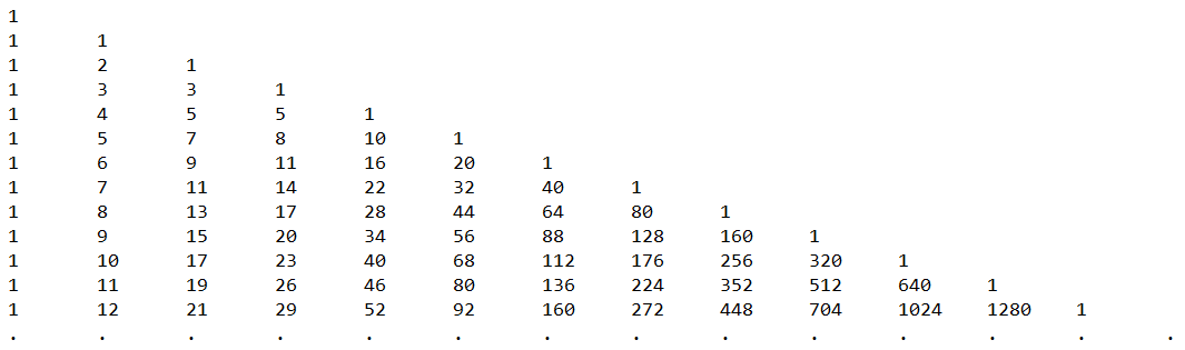
We shall motivate that further properties not included or studied in this paper reside within the structure of $\mathcal{T}$ – and accordingly $\mathcal{T}^{(y)}$ in that spirit for any finite $y\in\mathbb{R}_{+}\setminus\{0\}$ – which can be worked out analytically and/or numerically. For what follows, we shall focus our attention on $\mathcal{T}^{(1)}$ due to its probabilistic nature, which forms the initial motivation of this paper. First, in correspondence to the three main state-transition characteristics mentioned in Introduction, we collate three properties of $\mathcal{T}^{(1)}$ below, which are already shown in the previous section.

Remark 3.1.

The following properties hold for the matrix form of $\mathcal{T}^{(1)}\in\mathcal{M}^{\infty}$:

1. $\sup(\mathcal{T}^{(1)}_{n,*})=\mathcal{T}^{(1)}_{n,n}$ for every $n\geq 1$

2. $[\mathcal{T}^{(1)}_{n,n},\ldots,\mathcal{T}^{(1)}_{n,1}]$ is monotonically non-increasing for every $n\geq 1$

3. $\mathcal{T}^{(1)}_{n,n+k}=0$ for any $k\geq 2$ and every $n\geq 1$

The following charts demonstrate (i) the probability mass functions as one progresses from one row to the next over $\mathcal{T}^{(1)}$, (ii) the behaviour as one progresses from one finite column to the next over $\mathcal{T}^{(1)}$.

Figure 2: Left: First 50 probability mass functions from $\mathcal{T}^{(1)}$. Right: First 50 columns of $\mathcal{T}^{(1)}$

Here, we point to Remark 3.1 for patterns that can be observed from the left-panel of the chart. In addition, one can observe a form of symmetry across the rows and columns of $\mathcal{T}^{(1)}$ from Figure 2; the rows (i.e. probability mass functions) are left-skewed and the columns are right-skewed.

As an example, if the state-space of an associated near-log-concave random variable $X^{(n)}:\Omega\rightarrow\mathbf{D}^{(n,*)}$ for any $n\geq 2$ is given as follows:

$$\mathbf{D}^{(n,*)}\triangleq\{1,\ldots,n+1\},$$

then the $m$-th moment of $X^{(n)}$ is given by

$$\langle\textbf{M}\rangle_{\mathbf{D}^{(n,*)}}^{(m)}=\sum_{j=1}^{n+1}j^{m}\mu^{(n)}(j),$$ (36)

for any $n\geq 2$ and $m\geq 1$, if $\langle\textbf{M}\rangle_{\mathbf{D}^{(n,*)}}^{(m)}<\infty$. From (36), we shall highlight the following property for the first and second moments:

$$\langle\textbf{M}\rangle_{\mathbf{D}^{(n,*)}}^{(1)}\approx(n-2)+\frac{1}{4}\hskip 7.22743pt\text{for $n\geq 15$},$$

$$\langle\textbf{M}\rangle_{\mathbf{D}^{(n,*)}}^{(2)}\approx(n-2)^{2}+\frac{n+5}{2}+\frac{1}{4}\hskip 7.22743pt\text{for $n\geq 15$},$$

where both approximations sharpen progressively with increasing $n$. Therefore, the variance satisfies

$$\text{Var}^{\mu^{(n)}}\left[X^{(n)}\right]=\mathbb{E}^{\mu^{(n)}}\left[(X^{(n)})^{2}\right]-\mathbb{E}^{\mu^{(n)}}\left[(X^{(n)})\right]^{2}\approx\frac{59}{16}\hskip 7.22743pt\text{for $n\geq 15$}.$$ (37)

This suggests that the variance of $X^{(n)}$ converges to a constant as $n\rightarrow\infty$. From (37), we are motivated to present the following conjecture.

Conjecture 1.

Let $X^{(n,q)}:\Omega\rightarrow\mathbf{D}^{(n,q)}$ be a near-log-concave random variable with $\mathbf{D}^{(n,q)}=\{q,\ldots,n+q\}$ for any $q\in\mathbb{N}_{+}$, so that

$$\langle\textbf{M}\rangle_{\mathbf{D}^{(n,q)}}^{(m)}=\sum_{j=1}^{n+1}(j+q-1)^{m}\mu^{(n)}(j+q-1),$$

for any $n\geq 2$ and $m\in\{1,2\}$. Then, $\text{Var}^{\mu^{(n)}}\left[X^{(n,q)}\right]\rightarrow 59/16$ as $n\rightarrow\infty$, for any $q\in\mathbb{N}_{+}$.

We present the evolution of the Shannon entropy $\mathcal{S}^{(1,n)}$ over the rows of $\mathcal{T}^{(1)}$, and the Shannon sums $\mathcal{S}^{(y,n)}$ for some samples of $y\in[0.5,1]$, leading up to $\mathcal{S}^{(1,n)}$. Figure 3 displays at least three properties of the Shannon entropy evolution over $\mathcal{T}^{(1)}$: (i) non-decreasing, (ii) concave, and (iii) convergent.

Figure 3: Left: Shannon entropy $\mathcal{S}^{(1,n)}$. Right: Shannon sums $\mathcal{S}^{(y,n)}$ for samples $y\in[0.5,1]$

Regarding convergence, we note the numerical observation:

$$\lim_{n\rightarrow\infty}\mathcal{S}^{(1,n)}\approx 1.7907694690801...$$

Moreover, for any positive $y\leq 1$, Shannon entropy $\mathcal{S}^{(1,n)}$ is the only monotonically non-decreasing progression when compared to $\mathcal{S}^{(y,n)}$ with $y<1$. Although the properties of Shannon entropy can be studied analytically, we leave them for future.

3.1 Application in State Transitions

In physics and chemistry, state transitions refer to the transitioning of electrons between different energy levels, whereby electrons in atoms jump to lower states of energy by emitting photons, or jump to excited states of higher energy by absorbing photons – as the separation of states increases, the wavelength of emitted photons decreases. Such transitions are fundamentally important in spectroscopy for understanding how atoms interact with electromagnetic radiation.

Figure 4: Transitions over 100 timesteps. Left: Simulation of 2 paths. Right: Simulation of 50 paths

We simulate an atomic model using a Markov chain approach, whereby electron jumps are explained by the three state-transition characteristics encapsulated by stochastic-matrices in $\mathcal{M}^{\infty}$. Accordingly, an electron has the highest probability to remain at its current energy state over the next time step, as it is most probable that no photon will be emitted nor absorbed. Second, the atom is more likely to jump to a neighboring state of lower energy than to a distant state of lower energy. Finally, the system can absorb photons only to an extent that electrons can leap to neighboring excited states in one time step, and no further. From Proposition 2.30, we can choose any $\mathcal{T}^{(1)}(\mathbf{\lambda})\in\mathcal{M}^{\infty}$ for any $\lambda\in\mathcal{Q}$ for our purposes – we shall work with $\mathcal{T}^{(1)}(\mathbf{0})=\mathcal{T}^{(1)}$ for demonstration.

Due to the construct of $\mathcal{T}^{(1)}$, such a system is more likely to remain within lower energy states over its lifetime – more precisely, as the system achieves higher energy states, it gets increasingly less likely for electrons to jump to an even higher energy level. In addition, when the system jumps to a lower energy level, it is more likely to remain there, when compared to where it was. Hence, even if an electron manages to reach a very high energy state, it is expected that the system will gradually relax to lower energy levels by emitting more electromagnetic radiation than absorbing more photons. We call this the waterfall effect, which we demonstrate below.

Figure 5: Left: Conditioned to start from state = 10. Right: Conditioned to start from state = 50

In Figure 5, we condition the system at different energy levels and simulate 100 electron transition paths over 100 timesteps thereafter. The observed waterfall effect is due to the progression of $\mathcal{T}^{(1)}$, and different choices of $\lambda\in\mathcal{Q}$ for $\mathcal{T}^{(1)}(\mathbf{\lambda})\in\mathcal{M}^{\infty}$ will produce different electron transition patterns. More specifically, the waterfall effect arises for $\mathcal{T}^{(1)}$ since

$$\sum_{j=1}^{n-1}\mathcal{T}^{(1)}_{n,j}>\mathcal{T}^{(1)}_{n,n},$$

for every $n\geq 3$. In other words, the total probability for the system to transition downwards to any lower energy level is higher than the marginal probability of the system to remain at its current energy level for any $n\geq 3$.

Remark 3.2.

Note that $\mathcal{T}^{(1)}(\mathbf{1})$ for $\mathbf{1}=[1,1,...]$ provides the highest probabilities to achieve higher energy states amongst all possible $\mathcal{T}^{(1)}(\mathbf{\lambda})$. Hence, any $\lambda\in\mathcal{Q}$ can be used as a control variable on the waterfall effect mentioned above.

4 Conclusion

We introduced and studied an integer sequence progression that produces an infinite triangular array with numerous mathematical properties as presented in the main body of this work. Amongst several of these, the triangular array defines infinitely many degree sequences of multigraphs without loops, produces unimodal near-log-concave sequences, hosts a totally-positive Toeplitz matrix of order two, and naturally lends itself to a probabilistic setup through what we call near-log-concave random variables and their induced probability measures. We proved several asymptotic properties of the proposed triangular array to understand its convergent features. We showed that the triangular array can be taken as an anchor integer structure to construct infinitely many lower-triangular stochastic-matrices satisfying a particular set of state-transition characteristics, which can be observed in fields including atomic physics, cellular biology and queuing theory. As an application, we employed one of these transition matrices generated from the aforementioned triangular array in order to model and simulate state transitions involving electrons jumping from one energy level to another. In future, we shall investigate systems with such state-transition characteristics from a more holistic viewpoint, whereby the sequence progression presented in this paper forms a promising example. More specifically, we believe that studying infinite sequence progressions hosting particular characteristics as triangular arrays forms a viable direction to produce constructs towards modelling certain patterns observed in nature.

References

- [1] Hardy, G.H. A Theorem Concerning the Infinite Cardinal Numbers, Quart. J.Math., 35 (1904)
- [2] Shannon, C.E., A Mathematical Theory of Communication, Bell System Technical J., 27 (1948)
- [3] Davenport, H., Polya, G., On the Product of Two Power Series, Canadian J. Math, 1 (1949)
- [4] Kendall, D. G., Stochastic Processes Occurring in the Theory of Queues and their Analysis by the Method of the Imbedded Markov Chain, The Annals of Mathematical Statistics 24 (1953).
- [5] Jaynes, E.T., Information Theory and Statistical Mechanics, Physical Review, 106 (1957)
- [6] Hakimi, S., On the Realizability of a Set of Integers as Degrees of the Vertices of a Graph, SIAM J. Appl. Math. 10 (1962)
- [7] Read, R.C., An Introduction to Chromatic Polynomials, Journal of Combinatorial Theory 4 (1968)
- [8] Hoggar, S.G., Chromatic Polynomials and Logarithmic Concavity, J. Combinatorial Theory Ser. B, 16 (1974)
- [9] Joag-Dev, K., Proschan, F., Negative Association of Random Variables with Applications, Ann. Statistics (1983)
- [10] Brenti, F., Unimodal, Log-concave and Pólya Frequency Sequences in Combinatorics, American Mathematical Society (1989)
- [11] Stanley, R. P., Log-Concave and Unimodal Sequences in Algebra, Combinatorics, and Geometry, Annals of the New York Academy of Sciences (1989)
- [12] Cover, T., M., Thomas, J.A., Elements of Information Theory, Wiley (1991)
- [13] Hagedorn, G.A., Proof of the Landau-Zener Formula in an Adiabatic Limit with Small Eigenvalue Gaps, Commun. Math. Phys. 136 (1991)
- [14] Brenti, F., Expansions of Chromatic Polynomials and Log-Concavity, Trans. Amer. Math. Soc., 332 (1992)
- [15] Aharonov, Y., Davidovich, L., Zagury, N., Quantum random walks, Phys. Rev. A 48 (1993)
- [16] Brenti, F., Royle, G., Wagner, D., Location of Zeros of Chromatic and Related Polynomials of Graphs, Canad. J. Math., 46 (1994)
- [17] Hansen, N.F., Andersen, H.C., A New Formulation of Quantum Transition State Theory for Adiabatic Rate Constants, The Journal of Chemical Physics 101 (1994)
- [18] Cain, S.J., Chau, P.,C., Transition Probability Cell Cycle Model Part I—Balanced Growth, Journal of Theoretical Biology 185 (1997)
- [19] Seymour, P., Two Chromatic Polynomial Conjectures, Journal of Combinatorial Theory Series B, 70 (1997)
- [20] Gross, D., Harris, C. M., Fundamentals of Queueing Theory, John Wiley and Sons (1998)
- [21] MacKay, D.J.C., Information Theory, Inference, and Learning Algorithms, Cambridge University Press (2003)
- [22] Latorre, J.I., Orús, R., Adiabatic quantum computation and quantum phase transitions, Physical Review A 69 (2004)
- [23] Borgs, C., Absence of zeros for the chromatic polynomial on bounded degree graphs, Combin. Probab. Comput. 15 (2006)
- [24] Johnson, O., Goldschmidt, C., Preservation of Log-Concavity on Summation, ESAIM: Probability and Statistics 10 (2006)
- [25] Johnson, O., Log-concavity and the Maximum Entropy Property of the Poisson Distribution, Stochastic Processes and their Applications 117 (2007)
- [26] Fernández, R., Procacci, A., Regions Without Complex Zeros for Chromatic Polynomials on Graphs with Bounded Degree, Combin. Probab. Comput., 17 (2008)
- [27] Kempe, J., Quantum random walks: An introductory overview, Contemporary Physics 50 (2009)
- [28] Artalejo, J., Gomez-Corral, A., Markovian arrivals in stochastic modelling: a survey and some new results. Statistics and Operations Research Transactions 34 (2010)
- [29] Borda, M., Fundamentals in Information Theory and Coding, Springer (2011)
- [30] Huh, J., Milnor numbers of projective hypersurfaces and the chromatic polynomial of graphs, Journal of the American Mathematical Society 25 (2012)
- [31] Huh, J. Katz, E., Log-concavity of characteristic polynomials and the Bergman fan of matroids, Mathematische Annalen 354 (2012)
- [32] A., Saumard, J.A., Wellner, Log-concavity and strong log-concavity: A Review, Stat. Surv., 8 (2014)
- [33] Church, B.V., Williams, H.T., Mar, J.,Investigating skewness to understand gene expression heterogeneity in large patient cohorts, BMC Bioinformatics 20 (2019)
- [34] Lin, Z., Riemannian geometry of symmetric positive definite matrices via Cholesky decomposition, SIAM Journal on Matrix Analysis and Applications, 40 (2019)
- [35] Eur, C., Huh, J., Logarithmic Concavity for Morphisms of Matroids, Advances in Mathematics 367 (2020)
- [36] Huh, J., Matherne, J., Mészáros, K., Dizier, A., Logarithmic concavity of Schur and related polynomials, Transactions of the American Mathematical Society 375 (2022)
- [37] Berget, A., Spink, H., Tseng, D., Log-concavity of Matroid h-vectors and Mixed Eulerian Numbers, Duke Mathematical Journal (2023)
- [38] Marsiglietti, A., Pandey, P., A note on statistical distances for discrete log-concave measures, Statistics and Probability Letters 216 (2025)