Singular geometry and eigenframe topology in local rank-2 tensor observables

Abstract

Symmetric second-rank tensors are reported through magnitude-ordered principal values and axes. This representation folds tensor space: although the physical tensor remains smooth, the reported parameters develop cusps and exchange labels when one principal value crosses zero or two become degenerate. It conceals a global effect: an arrow chosen along a principal axis and transported continuously around a closed loop encircling a degeneracy can return with opposite orientation, even though the tensor returns to itself. This reversal defines a binary return parity that is invariant under smooth loop deformations that avoid degeneracy. We use the electric-field-gradient (EFG) tensor as a clean prototype because it is symmetric, traceless, and locally measurable at a probe site. Applied strain provides external control coordinates that steer the local EFG through tensor space, as determined from first-principles calculations. In rutile TiO₂, we identify an isolated control-space degeneracy with nontrivial parity; SnO₂ exhibits point- or line-like degeneracies depending on the control slice; and in cubic MgO, strain locally controls all five EFG components. These results distinguish local reporting singularities from global eigenframe topology. The underlying spectral geometry also applies to spatial tensor fields, and strain-tuned, orientation-resolved hyperfine spectroscopy offers a route to reconstruct return parity locally.

Figure 1: Sign reversal of a transported principal axis of the EFG tensor at the Ti site of rutile TiO₂, in the $Q_{B_{1g}}\,$-$\,Q_{B_{2g}}$ strain-control plane. The colour map shows the asymmetry parameter $\eta$; the black and white line segments show the two in-plane principal axes of the EFG tensor. Each principal axis is an axis without an arrow: $\overrightarrow{v}$ and $-\overrightarrow{v}$ are physically indistinguishable. The auxiliary arrows show one such axis after an arrow has been chosen and carried continuously around each of the two closed loops, labelled $C_{0}$ and $C_{1}$. We record the outcome of each loop by its return parity $w_{1}$: $w_{1}=0$ if the arrow returns as it started, and $w_{1}=1$ if it returns reversed. The loop $C_{1}$ encloses the degeneracy point (star; there $\eta=0$, two principal values coincide, and the axes become undefined), and the arrow returns reversed, giving $w_{1}(C_{1})=1$. The loop $C_{0}$ does not enclose the degeneracy point, and the arrow returns as it started, giving $w_{1}(C_{0})=0$. This parity is a binary topological property of the loop called the first Stiefel–Whitney invariant, and cannot be changed by any smooth choice of arrows. The $\eta=1$ ridges are intersections of the control plane with the ordering seam $\Delta_{0}$ of the reporting convention; they cause local relabellings but no sign reversal.

1 Spectral topology of local tensor observables

Symmetric second-rank tensors are among the most common observables in physics. Stress and strain in materials, diffusion tensors in imaging, magnetic-susceptibility and electrical-conductivity tensors in anisotropic media, and the hyperfine tensors of NMR, EPR, Mössbauer, and time-differential perturbed angular correlation (TDPAC) spectroscopy are all real symmetric $3\times 3$ tensors [Schroeder_J_2024, Funke_S_2021, Kaufmann_E_N_1979, Cho_H_2017, Basser_P_J_1994, Yan_H_2020]. In practice, such a tensor is almost never reported in full. It is diagonalized, its principal values are sorted by a convention, and the result is compressed into a small set of reported parameters such as the largest magnitude principal component $|V_{33}|$ and the asymmetry parameter $\eta$ [Kaufmann_E_N_1979, Harris_R_K_2008, Nardelli_F_2020]. We refer to any such reduced description as a chart: a coordinate system on the space of tensors, convenient for reporting but not guaranteed to be faithful everywhere. Diagonalization creates a representation with a geometry of its own.

The chart becomes problematic when the tensor is tracked continuously under temperature, strain or composition: smooth physical evolution can appear as sharp dips, cusps or label exchanges [Harris_R_K_2008, Derevianko_A_2026, Kanert_0_1988, PRB_paper]. Two distinct loci organize these artifacts. The first is the degeneracy stratum $\Sigma_{0}$, the subset of tensor space where two principal values are equal. There, the corresponding principal axes are no longer unique and $\eta=0$. The second is the determinant-zero set $\Delta_{0}$, where one principal value vanishes. Under magnitude ordering, $\Delta_{0}$ becomes an ordering seam: the reporting convention switches labels and $\eta=1$, even though the underlying tensor remains smooth and nondegenerate.

A subtler phenomenon appears for closed paths. Each principal axis of a symmetric tensor is an axis without an arrow: $\overrightarrow{v}$ and $-\overrightarrow{v}$ are physically indistinguishable, because each axis enters the tensor only through the product $\overrightarrow{v}\overrightarrow{v}^{T}$, which is blind to the sign. Suppose one nevertheless chooses an arrow along an axis and carries it continuously while the tensor is steered around a closed loop of control parameters (See Fig. 1). If the loop encloses a degeneracy point without crossing it, the arrow can return pointing the opposite way. This sign reversal was first noticed for electronic wavefunctions near intersecting molecular energy surfaces [von_Neumann_J_1929, Longuet_Higgins_H_C_1958, Herzberg_G_1963], and later understood as the real-symmetric counterpart of the Berry phase [Berry_M_V_1984]. This reversal defines a binary return parity $w_{1}\in\{0,1\}$ for the principal axis being followed. The parity cannot change under a smooth deformation of the loop unless an eigenvalue degeneracy is crossed. Mathematically, $w_{1}$ is the first Stiefel–Whitney invariant of that headless principal axis [von_Neumann_J_1929, Herzberg_G_1963, Ahn_J_2019]. Crucially, the tensor itself remains smooth and nondegenerate everywhere on the loop and the obstruction concerns only the continuous choice of an arrow along the headless principal axis. Any real symmetric rank-2 observable reported through principal values and principal axes carries an underlying spectral geometry, with the degeneracy strata, ordering seams, and an eigenframe defined only up to the sign choices of its headless axes [Delmarcelle_T_1994, Berry_Hannay_1977].

Unlike electronic band topology, which classifies Bloch wavefunctions over crystal-momentum space [Ahn_J_2019], the topology here belongs to the eigenframe of a single local tensor measured at one probe site and transported through a controlled parameter space. It emerges only when that tensor is followed around a closed loop, and requires neither quantum phase coherence nor a spatially extended state. To our knowledge, neither principal-axis anomalies nor $w_{1}$ have been treated in this way for a measurable, controllable local tensor observable.

The advance here is to realize this established topology in a strictly local, experimentally steerable tensor observable. The hyperfine electric field gradient (EFG) is an ideal platform [Schell_J_2017, Jerschow_A_2005, Liu_Y_S_1984]: it is exactly traceless, measured at a single probe site, strain-sensitive, and coupled to symmetry-adapted strain modes that provide natural control directions in its five-dimensional tensor space. A spectrally gapped strain loop around a degeneracy then forces a principal axis to accumulate an odd half-turn.

Using first-principles strain trajectories, we establish rutile TiO₂ as a prototype exhibiting local chart anomalies and a global sign-reversal loop, illustrate in SnO₂, how degeneracies can appear as points or lines depending on the chosen control plane, and demonstrate in MgO, complete local control of the traceless tensor space.

These results distinguish local cusps and label exchanges, produced when the ordered chart folds a smooth tensor trajectory, from the global sign reversal acquired when a headless principal axis is transported around a degeneracy. Taken together, these results establish strain-controlled EFGs as a local platform for observing and steering the singular geometry shared by symmetric rank-2 observables.

2 Principal-axis charts for electric field gradients

2.1 The ordered chart

The electric-field-gradient (EFG) tensor $\overleftrightarrow{V}\in X=\operatorname{Sym}_{0}(3,\mathbb{R})$ at the probe site $\overrightarrow{r_{0}}$ is the symmetric traceless part of the Hessian of the electrostatic potential $\Phi$ [Schatz_G_1996, Valenzuela_R_J_2025]:

$$V_{ij}=\left[\partial_{i}\partial_{j}\Phi-\frac{1}{3}\delta_{ij}\nabla^{2}\Phi\right]_{\overrightarrow{r}=\overrightarrow{r_{0}}}.$$ (1)

Symmetry follows from the equality of mixed partial derivatives, whereas tracelessness follows by construction. In a charge-free region, Poisson’s equation gives $\nabla^{2}\Phi=0$, and hence $V_{ij}=\partial_{i}\partial_{j}\Phi$. Consequently, $\overleftrightarrow{V}$ has five independent components. Throughout, the principal values of $\overleftrightarrow{V}$ are the eigenvalues $\lambda_{i}$ of its matrix representation. We use “principal values” in physical discussion and “eigenvalues” in formal statements.

Since $\overleftrightarrow{V}$ is real and symmetric, it admits an orthonormal eigenbasis, the principal-axis system (PAS): there exists $\overleftrightarrow{R}=(\overrightarrow{v_{1}},\overrightarrow{v_{2}},\overrightarrow{v_{3}})\in\mathrm{SO}(3,\mathbb{R})$, with columns the EFG eigenvectors, such that $\operatorname{diag}(V_{11},V_{22},V_{33})=\overleftrightarrow{R}^{T}\overleftrightarrow{V}\overleftrightarrow{R}$. The principal values are conventionally ordered by their absolute magnitudes,

$$|V_{33}|\geq|V_{22}|\geq|V_{11}|,$$ (2)

and the tensor is reported through the largest component $|V_{33}|$ and the asymmetry parameter [Schatz_G_1996, Valenzuela_R_J_2025, Kaufmann_E_N_1979, Harris_R_K_2008]

$$\eta=\frac{V_{11}-V_{22}}{V_{33}},$$ (3)

which satisfies

$$0\leq\eta\leq 1.$$ (4)

The pair $(|V_{33}|,\eta)$ retains the sorted spectrum but discards the orientation encoded in $\overleftrightarrow{R}$; it is the chart introduced in Section 1, and its two distinguished loci are characterized next.

2.2 The degeneracy stratum and ordering seam

A tensor lies in the degeneracy stratum $\Sigma_{0}\subset X$ when two principal values coincide, $V_{11}=V_{22}$. Tracelessness then forces the axial spectrum $(\lambda,\lambda,-2\lambda)$ up to ordering, so $\overleftrightarrow{V}\in\Sigma_{0}\Longleftrightarrow\eta=0$ (Eq. 3). On $\Sigma_{0}$, the repeated eigenvalue has a two-dimensional eigenspace: any orthonormal pair within it is an equally valid choice of axes, and the chart loses the corresponding frame directions. As the equality of two eigenvalues is a property of $\overleftrightarrow{V}$ itself, $\Sigma_{0}$ is independent of the chosen basis and reporting convention.

The determinant-zero set $\Delta_{0}\subset X$ consists of tensors for which one principal value vanishes, $\det(\overleftrightarrow{V})=V_{11}V_{22}V_{33}=0$. Under magnitude ordering, this means $V_{11}=0$, whereas $V_{22}=-V_{33}$ by tracelessness, so $\overleftrightarrow{V}\in\Delta_{0}\Longleftrightarrow\eta=1$ (Eq. 3). Thus, $\Delta_{0}$ appears as an ordering seam of the reported chart: crossing it forces a branch relabelling even though the underlying tensor is generically smooth and nondegenerate.

2.3 Relabelings and the eigenline

Crossing $\Delta_{0}$ exchanges the roles of $|V_{22}|$ and $|V_{33}|$ and produces the cusp-like seam at $\eta=1$, even though the tensor and its principal values remain smooth and nondegenerate. Around a closed path encircling $\Sigma_{0}$, the tensor returns to itself while the continuously transported frame may return only up to signs, for example

$$(\overrightarrow{v}_{1},\overrightarrow{v}_{2},\overrightarrow{v}_{3})\longrightarrow(-\overrightarrow{v}_{1},\overrightarrow{v}_{2},-\overrightarrow{v}_{3}).$$ (5)

No measurement distinguishes these frames. The spectral decomposition

$$\overleftrightarrow{V}=\sum_{i=1}^{3}\lambda_{i}\,\overrightarrow{v}_{i}\overrightarrow{v}_{i}^{\,T},\qquad(-\overrightarrow{v}_{i})(-\overrightarrow{v}_{i})^{T}=\overrightarrow{v}_{i}\overrightarrow{v}_{i}^{\,T},$$ (6)

shows that the tensor is built from the sign-free projectors of its eigenlines. Each PAS direction is an unoriented eigenline, thus the EFG is naturally described by headless principal axes. The sign choice in Eq. 5 is locally arbitrary, but continuous transport around a closed loop can return the chosen representative with the opposite sign. As formalized in the next section, this defines a topologically nontrivial holonomy.

3 Spectral-geometric framework

We now work directly in the invariant tensor space $X=\mathrm{Sym}_{0}(3,\mathbb{R})$, equipped with the Frobenius inner product $\langle A,B\rangle_{F}=\operatorname{tr}(A^{\top}B)$, and study the EFG as a function of one or two control parameters chosen from symmetry-adapted strain modes of the crystal. Any symmetric strain tensor decomposes into an isotropic trace component and a traceless deviatoric component; the latter, expanded in a symmetry-adapted basis, provides the local control directions used to navigate $X$. In this intrinsic formulation, chart anomalies can be described without committing to a particular ordering convention, connecting the Herzberg–Longuet-Higgins holonomy structure of real-symmetric eigenproblems [Longuet_Higgins_H_C_1958, Herzberg_G_1963, Berry_M_V_1984] with the shape-space description familiar from traceless order parameters and deviatoric strain [de_Gennes_P_G_1993, Beris_A_N_1994].

For a fully geometric interpretation of the EFG tensor, the ordered PAS parameters introduced in section 2 are insufficient, since they depend on a particular eigenvalue ordering and principal-axis convention. Instead, the relevant basis-independent quantities are the polynomial invariants of $\overleftrightarrow{V}$.

The quadratic invariant

$$I_{2}=\operatorname{Tr}\left(\overleftrightarrow{V}^{\,2}\right)=\left\|\overleftrightarrow{V}\right\|_{F}^{2},$$ (7)

gives the overall basis-independent magnitude of the EFG tensor, while the cubic invariant [de_Gennes_P_G_1993, Beris_A_N_1994]

$$I_{3}=\operatorname{Tr}\left(\overleftrightarrow{V}^{\,3}\right)=3\det\left(\overleftrightarrow{V}\right),$$ (8)

encodes the signed shape of its eigenvalue spectrum. In particular, the determinant-zero set $\Delta_{0}$ is characterized by $I_{3}=0$ and in the magnitude-ordered PAS chart, this set appears as the ordering seam $\eta=1$.

It is useful to introduce the dimensionless normalized shape parameter

$$p=\sqrt{6}\,\frac{I_{3}}{I_{2}^{3/2}}.$$ (9)

The prefactor $\sqrt{6}$ normalizes the axial limits to $p=\pm 1$. For an axial spectrum $(\lambda,\lambda,-2\lambda)$, one has $I_{2}=6\lambda^{2}$ and $I_{3}=-6\lambda^{3}$, so $p=-\operatorname{sgn}(\lambda)$. Thus, $p$ describes the signed spectral shape independently of tensor magnitude and basis: $p=\pm 1$ on the degeneracy stratum $\Sigma_{0}$ $(\eta=0)$, while $p=0$ on the determinant-zero set $\Delta_{0}$, which forms the $\eta=1$ ordering seam of the magnitude-ordered chart.

The two loci govern different regularity domains: the eigenframe is well defined on $X\setminus\Sigma_{0}$, whereas the ordered chart is smooth only on $X\setminus(\Sigma_{0}\cup\Delta_{0})$. Local chart anomalies arise when a trajectory approaches or crosses either locus; global holonomy arises only when a closed loop links the relevant component of $\Sigma_{0}$. We separate the resulting structure into two linked forms.

I) The chart-wall form: local singular geometry.

Let $y\mapsto\overleftrightarrow{V}(y)\in X$ be a smooth tensor trajectory. Since $I_{2}$ and $I_{3}$ are polynomial invariants of $\overleftrightarrow{V}$, they vary smoothly along the trajectory. Nevertheless, the ordered PAS coordinates $(|V_{33}|,\eta)$ can exhibit sharp, convention-induced features when the trajectory approaches or crosses either of the two distinguished loci, $\Sigma_{0}$ or $\Delta_{0}$.

To visualize this local chart-wall structure, we restrict to a fixed tensor magnitude $I_{2}$. Since the tensor is traceless, fixing $I_{2}$ leaves only one independent degree of freedom in the spectral shape. We parameterize this degree of freedom by an angular coordinate, defined through eq. 9:

$$p=\cos(3\delta),$$ (10)

The coordinate $\delta$ provides a smooth invariant description of the eigenvalue spectrum, while the reported PAS coordinates reveal how $\eta$ approaches the chart boundaries $\eta=0$ and $\eta=1$ near $\Sigma_{0}$ and $\Delta_{0}$ respectively, see Fig. 2.

II) The holonomy form: global topology.

Let $C$ be a closed control loop with $\overleftrightarrow{V}(C)\subset X\setminus\Sigma_{0}$. Such a spectrally gapped loop contains no principal-value degeneracy, so each axis can be followed continuously. We denote the return parity of one tracked axis by $w_{1}(C)$; the complete biaxial frame has richer topology.

If a spectrally gapped loop $C$ links the relevant component of $\Sigma_{0}$, a chosen arrow along the principal axis can be transported continuously, yet return reversed after one circuit. This gives the nontrivial parity $w_{1}(C)=1$, even though the tensor remains nondegenerate everywhere on $C$: the obstruction is global and arises because the loop links a degeneracy where the axis itself becomes undefined. By contrast, crossing $\Delta_{0}$ leaves the principal values and eigenlines smooth, but forces the magnitude-ordering convention to exchange their labels, producing a local cusp-like feature at $\eta=1$ without changing the eigenline topology. Thus, $\Sigma_{0}$, rather than $\Delta_{0}$, controls the global return parity shown in Fig. 1.

Figure 2: Local chart-wall structure of the ordered PAS representation at fixed tensor magnitude $I_{2}$. (a) The normalized principal values vary smoothly as a function of the invariant shape angle $\delta$ (see Eq. 10). The endpoints $\delta=0$ and $\delta=\pi/3$ lie on the degeneracy stratum $\Sigma_{0}$, where two principal values coincide, and the ordered PAS parameter satisfies $\eta=0$. At $\delta=\pi/6$, one principal value vanishes ($\lambda_{2}=0$), corresponding to the ordering seam $\Delta_{0}$. (b) After imposing the ordered PAS convention, the smooth spectrum is folded into piecewise branches for $|V_{11}|,|V_{22}|,|V_{33}|$. The magnitude ordering $|V_{33}|\geq|V_{22}|\geq|V_{11}|$ forces branch reassignments at the chart walls. In particular, crossing $\Delta_{0}$ gives $|V_{11}|=0$ and $|V_{22}|=|V_{33}|$, producing the $\eta=1$ seam. By contrast, approaching $\Sigma_{0}$ drives the spectrum to the axial limit, where two principal values coincide ($|V_{11}|=|V_{22}|$) and $\eta=0$. At this boundary the corresponding two-dimensional eigenspace is degenerate, so the associated PAS directions are no longer uniquely defined. (c) Comparison between the ordered PAS asymmetry parameter $\eta$ and the smooth invariant shape coordinate $p=\cos(3\delta)$. While $p$ varies smoothly from $+1$ to $-1$, the parameter $\eta$ is folded between the axial boundary $\eta=0$, governed by $\Sigma_{0}$, and the ordering seam $\eta=1$, governed by $\Delta_{0}$. This shows that $(|V_{33}|,\eta)$ is a convenient ordered chart, but not a globally smooth geometric representation of the EFG tensor space.

4 Isolated eigenframe holonomy in rutile TiO₂

For the Ti site in rutile TiO₂, the symmetry-adapted controls $Q_{B_{1g}}$ and $Q_{B_{2g}}$ define a two-dimensional control slice in $X=\mathrm{Sym}_{0}(3,\mathbb{R})$ passing through the unstrained DFT EFG tensor:

$$\overleftrightarrow{V}_{0}=\begin{pmatrix}V_{xx,0}&V_{xy,0}&0\\ V_{yx,0}&V_{yy,0}&0\\ 0&0&V_{zz,0}\end{pmatrix},$$ (11)

with $V_{xy,0}=V_{yx,0}$ and $V_{xx,0}+V_{yy,0}+V_{zz,0}=0$. The applied strain tensor is written as

$$\overleftrightarrow{\varepsilon}(Q_{B_{1g}},Q_{B_{2g}})=Q_{B_{1g}}\,\widehat{\varepsilon}_{B_{1g}}+Q_{B_{2g}}\,\widehat{\varepsilon}_{B_{2g}},$$ (12)

where

$$\widehat{\varepsilon}_{B_{1g}}=\begin{pmatrix}1&0&0\\ 0&-1&0\\ 0&0&0\end{pmatrix},\qquad\widehat{\varepsilon}_{B_{2g}}=\begin{pmatrix}0&1&0\\ 1&0&0\\ 0&0&0\end{pmatrix}.$$ (13)

For each point $(Q_{B_{1g}},Q_{B_{2g}})$ in this strain-control plane, the DFT calculation defines an EFG response

$$\overleftrightarrow{V}=\overleftrightarrow{V}(Q_{B_{1g}},Q_{B_{2g}})\in X.$$ (14)

To leading order about the unstrained structure,

$$\begin{split}\overleftrightarrow{V}(Q_{B_{1g}},Q_{B_{2g}})={}&\overleftrightarrow{V}_{0}+Q_{B_{1g}}\left.\frac{\partial\overleftrightarrow{V}}{\partial Q_{B_{1g}}}\right|_{(Q_{B_{1g}},Q_{B_{2g}})=(0,0)}\\ &+Q_{B_{2g}}\left.\frac{\partial\overleftrightarrow{V}}{\partial Q_{B_{2g}}}\right|_{(Q_{B_{1g}},Q_{B_{2g}})=(0,0)}+\mathcal{O}\bigl(\|(Q_{B_{1g}},Q_{B_{2g}})\|^{2}\bigr).\end{split}$$ (15)

The derivatives are the strain–EFG responses along the two symmetry-adapted control directions.

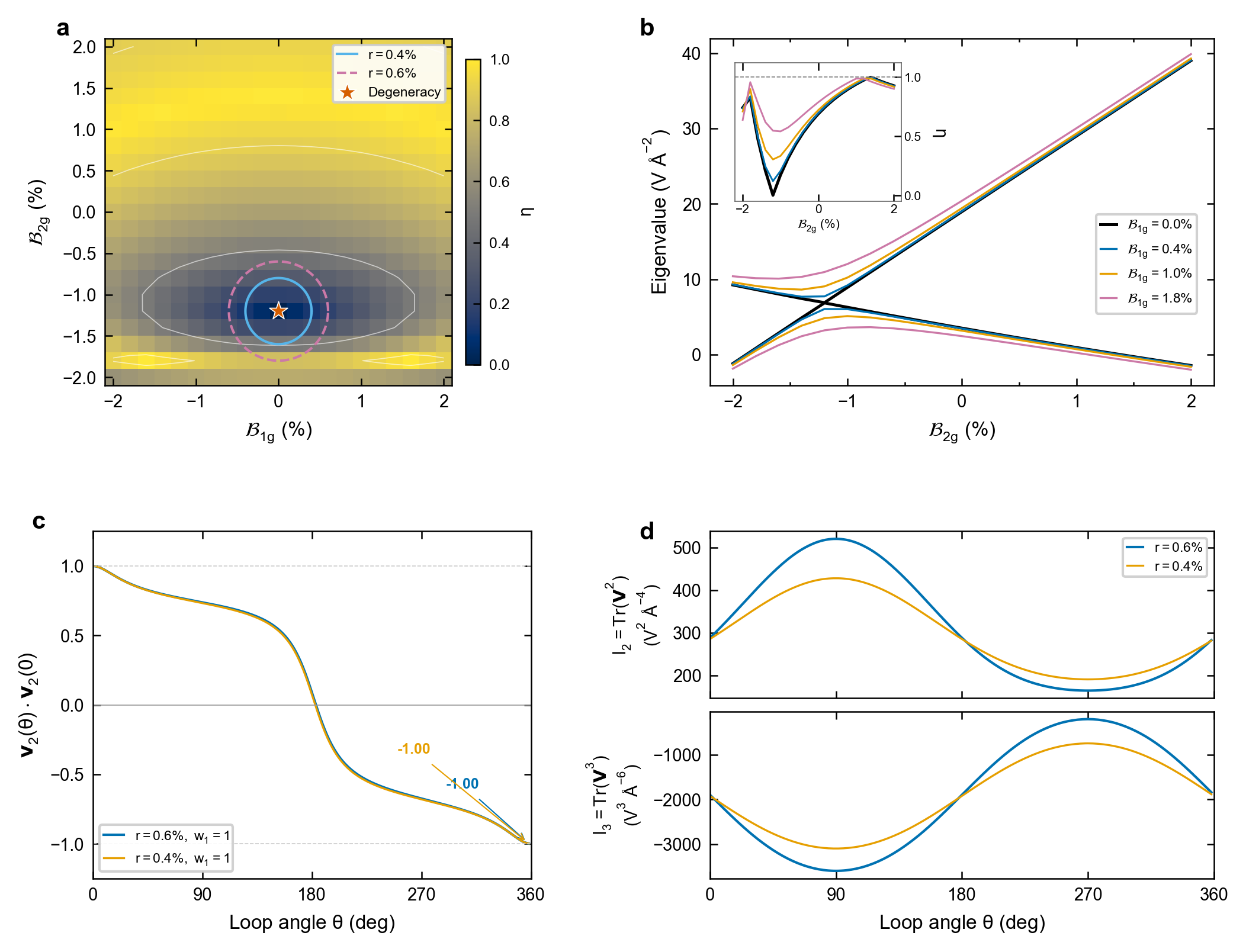
In this slice, the map of $\eta$ over the control plane (Figs. 1 and 3a) reveals an isolated point where two principal values coincide. Fits to the Cartesian EFG components show that $V_{xx}=V_{yy}$ and $V_{xy}=0$ at a single strain point. The nonzero Jacobian there confirms that the $Q_{B_{1g}}\,$-$\,Q_{B_{2g}}$ strain plane crosses the degeneracy stratum $\Sigma_{0}$ transversely (Methods). This single point supplies both forms of Section 3. Locally, it is a conical intersection: one-dimensional cuts show principal-value branches that exchange character, with avoided crossings on cuts that miss the point and the axial limit $\eta=0$ on the cut through it (Fig. 3b). Globally, a cut through $\Sigma_{0}$ carries no invariant, because the frame is singular at the degeneracy itself. The return parity becomes well defined once the cut is opened into a closed, spectrally gapped loop $C$ around the point. The transported arrows around the loops $C_{0}$ and $C_{1}$ are shown directly in Fig. 3c, while the invariants $I_{2}$ and $I_{3}$ vary smoothly (Fig. 3d), showing that the orientation reversal is global while the trajectory remains spectrally gapped. Thus, rutile TiO₂ realizes both the chart-wall form and the holonomy form from first principles.

Figure 3: Return parity of the EFG eigenframe in the $Q_{B_{1g}}\,$-$\,Q_{B_{2g}}$ strain-control plane of rutile TiO₂. (a) The colour map shows the asymmetry parameter $\eta$. A point degeneracy of two principal values (star) is reached under the symmetry-adapted strains. Two closed, spectrally gapped loops $C$ of different radii are shown in blue and dashed orange. Locally, $\eta$ indicates proximity to the degeneracy, while the loop invariant $w_{1}(C)$ detects whether the closed path encircles it; smooth deformations of a gapped, encircling loop do not change $w_{1}(C)$. (b) EFG principal values along cuts at several fixed values of $Q_{B_{1g}}$. Near the degeneracy, two principal-value branches approach and exchange character, the local chart-wall signature of the degeneracy stratum $\Sigma_{0}$; the inset shows the corresponding dip of $\eta$ toward the axial limit $\eta=0$. The avoided crossings seen in one-dimensional cuts arise from an isolated conical intersection, or diabolical point, in the full control plane. The local structure resembles a tilted Dirac cone, except that the surfaces represent EFG principal values rather than electronic bands. (c) Normalized overlap $\vec{v}_{2}(\theta)\cdot\vec{v}_{2}(0)$, where $\vec{v}_{2}$ is a continuously choosen arrow along the selected principal axis. After one full circuit, $\theta=2\pi$, the overlap approaches $-1$ rather than $+1$: the arrow returns reversed, $w_{1}(C)=1$. The same behaviour for both loop radii confirms the topological robustness of the parity. (d) Basis-independent invariants $I_{2}$ and $I_{3}$ along the same loops. Both vary smoothly, confirming that the sign reversal is not caused by any singularity of the underlying tensor trajectory, but by the global topology of eigenframe transport around the degeneracy stratum.

5 Slice-dependent degeneracy structure in SnO₂

Compared with TiO₂, the SnO₂ control plane displays a richer degeneracy structure. In the $Q_{B_{1g}}\,$-$\,Q_{B_{2g}}$ slice, two distinct intersections with the discriminant stratum $\Sigma_{0}$ are observed. The first is an isolated point degeneracy, where $\lambda_{2}=\lambda_{3}$, analogous to the degeneracy found in TiO₂. The second is an extended degeneracy branch, where $\lambda_{1}=\lambda_{2}$. Both features correspond to axially symmetric EFG tensors and thus, to the ordered PAS limit $\eta=0$, but they have different geometrical roles within the chosen two-dimensional control slice, as shown in Fig. 4(a).

The extended branch is protected within the restricted $Q_{B_{1g}}\,$-$\,Q_{B_{2g}}$ control plane. These two controls preserve the $xy\oplus z$ block structure of the EFG tensor (Eq. 11), so that $V_{xz}=V_{yz}=0$ and the $z$-like principal direction remains decoupled from the in-plane subspace. This symmetry-enforced decoupling allows the $z$-like and in-plane principal values to cross without level repulsion. Hence, within the two-dimensional control plane, the degeneracy condition can define a continuous line. An $E_{g}$-type $xz$ or $yz$ control couples the two sectors, lifts the degeneracy locally, and permits a spectrally gapped loop in a plane transverse to the degeneracy line.

The isolated point admits a gapped encircling loop with $w_{1}(C)=1$. The extended branch cannot be encircled in the same slice without crossing $\Sigma_{0}$, where the frame is singular, so its loop parity is unresolved there (Fig. 5).

Therefore, SnO₂ demonstrates that the observed structure depends both on the material and on how the control slice intersects the singular set: the same geometry appears as an encirclable point or a line of pinned $\eta=0$ (Figs. 4 and 5).

Figure 4: Chart-wall structure of the EFG tensor in the $Q_{B_{1g}}\,$-$\,Q_{B_{2g}}$ strain-control plane of rutile SnO₂. (a) Colour map of the asymmetry parameter $\eta$. The star marks an isolated $\lambda_{2}=\lambda_{3}$ degeneracy point; the blue curve marks an extended $\lambda_{1}=\lambda_{2}$ degeneracy branch. The isolated point behaves analogously to the TiO₂ case, whereas the extended branch shows that, in this two-dimensional control slice, the $\lambda_{1}=\lambda_{2}$ degeneracy is not fully lifted by the available strain controls. (b) EFG principal values along cuts at several fixed values of $Q_{B_{1g}}$. Near the isolated point, the principal-value branches reproduce the conical-intersection structure found in TiO₂. in contrast, the $\lambda_{1}=\lambda_{2}$ degeneracy forms a continuous curve because the restricted control plane preserves the $xy\oplus z$ block structure. An additional $E_{g}$-type $xz$ or $yz$ control would introduce the off-block coupling needed to lift the crossing locally. (c) Ordered PAS magnitudes $|V_{11}|,|V_{22}|,|V_{33}|$ along the same cuts: the magnitude-ordering convention forces label reassignments, producing sharp, non-smooth branches even though the underlying tensor varies smoothly. (d) Asymmetry parameter $\eta$ along the same cuts. Values $\eta\to 0$ signal approach to the degeneracy stratum $\Sigma_{0}$; in contrast to the isolated point, the extended branch produces a region where $\eta$ remains pinned at zero, because the trajectory can follow the degeneracy set over a finite interval rather than crossing it at a single point. Values $\eta\to 1$ signal crossing of the ordering seam $\Delta_{0}$, where one principal value vanishes. Overall, SnO₂ illustrates the distinction between isolated and extended intersections with $\Sigma_{0}$: isolated intersections appear as points that can carry loop parity, while extended intersections appear as lines of pinned $\eta=0$ that no spectrally gapped loop within the same two-dimensional plane can locally encircle, so the return parity is not resolved in this slice.

Figure 5: The SnO₂ EFG eigenframe field in the $Q_{B_{1g}}\,$-$\,Q_{B_{2g}}$ control plane. The colour map shows the asymmetry parameter $\eta$; the black and white headless line segments show the two in-plane principal axes of the EFG tensor. Both an isolated point degeneracy and an extended degeneracy branch are visible. The isolated point acts as a winding centre for the headless axes: the frame winds by half a turn per circuit, the field pattern of nontrivial return parity, $w_{1}=1$. In contrast, the extended branch appears as a line of singular frames along which $\eta=0$ remains pinned. Any loop attempting to encircle the branch within this two-dimensional slice must cross the degeneracy stratum $\Sigma_{0}$, where the frame is undefined, so no spectrally gapped loop exists around it and the return parity is not resolved in this slice. Leaving this plane through an $E_{g}$-type control would permit a gapped loop transverse to the branch. The $\eta=1$ regions are ordering seams $\Delta_{0}$ of the reporting convention and do not represent degeneracies of the principal values.

6 Complete local tensor control in cubic MgO

MgO provides a clean, high-symmetry example in which strain acts as a local control field for the EFG tensor. In the unstrained cubic reference structure, the Mg site has cubic symmetry, so the EFG vanishes, $\overleftrightarrow{V}_{0}=\overleftrightarrow{0}$. Consequently, the basis-independent invariants $I_{2}$ and $I_{3}$ also vanish, and the PAS is not uniquely defined at the cubic point.

As summarized in the symmetry-adapted basis construction in the Methods section, the symmetric strain tensor decomposes into an isotropic $A_{1g}$ trace component and a five-dimensional traceless deviatoric sector. The $A_{1g}$ component changes the volume but preserves the cubic site symmetry. Hence, it does not define an independent traceless EFG direction. By contrast, the $E_{g}$ and $T_{2g}$ deviatoric strain modes transform in the same symmetry-adapted rank-2 tensor basis as the EFG tensor. Thus, excluding the isotropic trace mode, the strain basis and the EFG basis are naturally matched by symmetry.

Near the cubic reference point, the strain-induced EFG can be described by the linear response:

$$V_{ij}=\sum_{\alpha}\frac{\partial V_{ij}}{\partial\epsilon_{\alpha}}\epsilon_{\alpha}+\mathcal{O}(\epsilon^{2}),$$ (16)

where $i,j\in{x,y,z}$, and $\epsilon_{\alpha}$ denotes the amplitude of a symmetry-adapted strain mode. Thus, the derivative $\partial V_{ij}/\partial\epsilon_{\alpha}$ measures the response of the Cartesian EFG component $V_{ij}$ to the mode amplitude $\epsilon_{\alpha}$, rather than to an individual Cartesian strain component. After excluding the isotropic $A_{1g}$ trace mode and vectorizing the five independent traceless EFG components, this response defines a $5\times 5$ susceptibility matrix. The calculated matrix is full rank to numerical accuracy, indicating that the symmetry-adapted deviatoric strain modes form a complete local control basis for $X=\mathrm{Sym}_{0}(3,\mathbb{R})$.

The MgO results provide a constructive realization of the framework: suitable strain trajectories can target singular PAS features while locally controlling the EFG magnitude $I_{2}$ and spectral shape $p$ (or $\eta$).

Figure 6: Local strain control of the EFG tensor in cubic MgO. (a) $\eta$-shadow maps for several two-dimensional slices of the strain-control space, each spanned by a different pair of symmetry-adapted strain modes. White dots and dashed/solid lines mark intersections with the degeneracy stratum $\Sigma_{0}$, where two principal values coincide and the ordered PAS parameter approaches the axial limit $\eta=0$. The different slices show that the same underlying singular structure can appear as isolated points, extended lines, or symmetry-pinned regions depending on the chosen strain-mode pair. (b) Corresponding PAS footprints in the $(|V_{33}|,\eta)$ representation. Each footprint records the range of reported asymmetry values accessible as the EFG magnitude changes under a given strain-mode pair. The star marks the unstrained cubic reference point, where $\overleftrightarrow{V}=0$; at this point all principal values coincide and the PAS is undefined. The different footprints demonstrate that the path traced in the ordered chart depends strongly on the selected strain trajectory. (c) Diagonal cuts through the two-mode control planes of panel (a): $|V_{33}|$ (upper) and $\eta$ (lower) as functions of strain amplitude. Depending on the strain-mode pair, the trajectory may approach the degeneracy stratum $\Sigma_{0}$, producing dips toward $\eta=0$, or cross the ordering seam $\Delta_{0}$, producing cusp-like structures near $\eta=1$ — sharp reported behaviour arising from smooth tensor trajectories encountering these two distinguished loci. (d) Component-resolved linear response $\partial V_{ij}/\partial\epsilon_{\alpha}$, where $\epsilon_{\alpha}$ is the amplitude of a symmetry-adapted strain mode. The map shows how each mode steers the Cartesian EFG components, and the side plots show representative component evolutions under individual mode strains.

7 Tensor observables beyond the EFG

This spectral geometry is not specific to EFGs. In many fields, the same singular geometry is hidden by projecting a symmetric tensor to scalar anisotropies, selected principal values, directors, or auxiliary orientation angles. Shielding and quadrupolar tensors in NMR, zero-field-splitting tensors in EPR, diffusion tensors in imaging, and the deviatoric parts of stress and strain are all reported through ordered charts of this kind. Each community’s sorting convention places its ordering seams at different locations, but the degeneracy stratum $\Sigma_{0}$ and the return parity $w_{1}$ are convention-independent. Therefore, tracked tensor data in these fields can be reinterpreted as trajectories in tensor space, with chart artifacts marking local singular geometry and closed control loops revealing possible eigenframe parity.

A natural next step combines hyperfine spectroscopy with multi-axis piezoelectric strain control [Hicks_C_W_2014, Barber_M_E_2019]. Return parity requires the frame, and not only $(|V_{33}|,\eta)$: fixed-geometry single-crystal TDPAC resolves the orientation discarded by powder averaging, as do single-crystal NMR rotation patterns [Fojud_Z_2007, Kissikov_T_2017, Kawamura_M_2010]. Likewise, angle-dependent single-crystal Mössbauer line intensities determine the EFG axes in ¹¹⁹Sn absorbers [Szymanski_K_2018, Negita_H_1977]. A complementary native-site route is thermal-neutron activation of enriched ¹¹⁸SnO₂, which produces ^119mSn directly on the host Sn sublattice [Hannaford_P_1965, Hannaford_P_1969]. In a thin single-crystal specimen, orientation-resolved $e^{-}$–$\gamma$ TDPAC could exploit the strongly converted ^119mSn cascade [Soares_J_C_1973, Schell_J_2017] to follow the Sn-site EFG eigenframe under strain. In either implementation, an additional $E_{g}$-type strain could define a spectrally gapped loop transverse to the protected degeneracy branch.

Experimentally, one follows the fitted principal-axis projector around enclosing and non-enclosing loops and tests whether parallel transport accumulates odd or even half-turn parity (Fig. 1). The broader challenge is to move from reading low-dimensional slices to designing higher-dimensional tensor trajectories with prescribed singular and topological signatures.

Data availability

The first-principles data supporting this study, including the calculated EFG tensors, strain-control trajectories, eigenvalue/eigenframe data, and raw DFT output files, will be deposited in a public repository before publication. Repository accession information and persistent identifiers will be added to the final version of the manuscript. Data are available from the corresponding author upon reasonable request during review.

Supplementary information

This manuscript is intended to be self-contained. No supplementary information is provided at this stage.

Acknowledgements

Financial support was provided by the Federal Ministry of Research, Technology, and Space (BMFTR) through Grants No. 05K16PGA, 05K22PGA, 05K25PGA, and 05K22PGB; by the ISOLDE Collaboration; by the EU Horizon Europe Programme under Grant Agreement No. 101057511 (EURO-LABS); and by the Foundation for Science and Technology, Portugal, under Grant No. CERN-FIS-PAR-0005-2017.

Computational resources were provided by the Polish PLGrid Infrastructure through ACK Cyfronet AGH under Grant No. PLG/2023/016756. The authors also acknowledge computing time granted by the Center for Computational Sciences and Simulation (CCSS) of the University of Duisburg-Essen and provided on the supercomputer amplitUDE at the Zentrum für Informations- und Mediendienste (ZIM), funded through DFG project 459398823, grant ID INST 20876/423-1 FUGG.

Declarations

Competing interests

The authors declare no competing interests.

Author contributions

B.D., S.Q.J. and I.C.J.Y. contributed equally to this work. Co-first author ordering is in descending order of seniority. H.C.H., D.C.L., A.K. and J.H.S. supervised this work equally. Co-senior author ordering was determined by mutual agreement.

I.C.J.Y. conceived the spectral-geometric and topological framework, developed the theoretical interpretation, performed the eigenframe-holonomy analysis, prepared the manuscript structure, and wrote the original draft. S.Q.J. performed the first-principles calculations, developed and implemented the strain-control workflows, analysed the calculated EFG tensors, and contributed to data visualization and interpretation. B.D. contributed to the conceptual development, theoretical analysis, figure preparation, and interpretation of the tensor-space and eigenframe-topology results.

T.T.D. contributed to the hyperfine-spectroscopy interpretation, validation of the physical setting, and critical revision of the manuscript. P.M.S. contributed to discussion of the hyperfine-spectroscopy context, interpretation of local EFG observables, and critical revision of the manuscript.

H.C.H., D.C.L., A.K. and J.H.S. supervised the project, contributed to interpretation of the results, provided scientific guidance, and revised the manuscript critically. All authors discussed the results and approved the final manuscript.

Methods

(A) Invariant parametrization of traceless EFG spectra

We represent the EFG at the probe site by a real symmetric traceless tensor $\overleftrightarrow{V}\in X=\operatorname{Sym}_{0}(3,\mathbb{R})$, and characterized its spectrum using the quadratic and cubic rotation invariants:

$$I_{2}=\operatorname{Tr}(\overleftrightarrow{V}^{2}),\qquad I_{3}=\operatorname{Tr}(\overleftrightarrow{V}^{3}).$$ (M1)

For traceless $3\times 3$ tensor, $I_{3}=3\det(\overleftrightarrow{V})$.

The characteristic polynomial can be written in the invariant form as:

$$\chi_{\overleftrightarrow{V}}(\lambda)=\det(\lambda\overleftrightarrow{Id}-\overleftrightarrow{V})=\lambda^{3}-\frac{I_{2}}{2}\lambda-\frac{I_{3}}{3},$$ (M2)

so the principal values $\{\lambda_{i}\}_{i\in\{1,2,3\}}$ are the real roots of the depressed cubic.

To detect eigenvalue degeneracies, we use the polynomial discriminant of the characteristic cubic:

$$\operatorname{disc}\overleftrightarrow{V}=\frac{1}{2}I_{2}^{3}-3I_{3}^{2}=\prod_{i<j}(\lambda_{i}-\lambda_{j})^{2},$$ (M3)

which vanishes if and only if two eigenvalues coincide.

This singles out the discriminant, or degeneracy, stratum:

$$\Sigma_{0}:=\{\overleftrightarrow{V}\in X\mid\operatorname{disc}\overleftrightarrow{V}=0\}\equiv\{\overleftrightarrow{V}\in X\mid\exists i\neq j,\lambda_{i}=\lambda_{j}\},$$ (M4)

and the determinant-zero set:

$$\Delta_{0}:=\{\overleftrightarrow{V}\in X\mid\det\overleftrightarrow{V}=0\}\equiv\{\overleftrightarrow{V}\in X\mid\exists i,\lambda_{i}=0\}.$$ (M5)

The set $\Sigma_{0}$ is intrinsic to tensor space because it is defined by the equality of two eigenvalues, independently of the chosen basis or principal-value ordering. Likewise, the set $\Delta_{0}$ is defined invariantly, but its role as an ordering seam arises only after the magnitude-ordering convention is imposed.

For a scale-shape decomposition, we define the dimensionless invariant ratio:

$$p:=\frac{\sqrt{6}I_{3}}{I_{2}^{1.5}}\in[-1,1],\qquad\delta(p):=\frac{1}{3}\cos^{-1}(p)\in\left[0,\frac{\pi}{3}\right].$$ (M6)

The trigonometric solution for $\chi(\overleftrightarrow{V})=0$ gives via Cardano [NIST_Cubic_Equations_2025]:

$$\lambda_{k}=2\sqrt{\frac{I_{2}}{6}}\cos\left(\delta(p)+\frac{2\pi k}{3}\right),\qquad k\in\{0,1,2\},$$ (M7)

and we use the principal branch $\delta\in[0,\pi/3]$ for a unique shape parameter. The trigonometric roots are obtained up to permutation; we then sort them to enforce the signed ordering $\lambda_{1}\leq\lambda_{2}\leq\lambda_{3}$:

$$\lambda_{1}=2\sqrt{\frac{I_{2}}{6}}\cos\left(\delta+\frac{2\pi}{3}\right),\qquad\lambda_{2}=2\sqrt{\frac{I_{2}}{6}}\cos\left(\delta+\frac{4\pi}{3}\right),\qquad\lambda_{3}=2\sqrt{\frac{I_{2}}{6}}\cos(\delta).$$ (M8)

(B) Closed-form mapping from invariants to the PAC chart $(|V_{33}|,\eta)$

Because the PAC convention orders principal values by absolute magnitude, $(|V_{33}|,\eta)$ is obtained by composing the smooth invariant map $\overleftrightarrow{V}\rightarrow(I_{2},I_{3})$ with a piecewise PAS labelling rule. Following equations M6 to M8, the PAC largest absolute component is:

$$|V_{33}|:=\max_{i\in\{1,2,3\}}|\lambda_{i}|.$$ (M9)

The principal value associated with $|V_{33}|$ switches at $\delta=\pi/6$, where the determinant-zero set becomes the ordering seam of the magnitude-ordered chart:

$$\delta=\frac{\pi}{6}\Leftrightarrow|\lambda_{3}|=|\lambda_{1}|\Leftrightarrow\lambda_{2}=0\Leftrightarrow\det(\overleftrightarrow{V})=0\Leftrightarrow I_{3}=0\ (p=0).$$ (M10)

A compact way to encode the folding induced by the absolute-magnitude assignment is to define the folded angle:

$$\delta_{*}(p):=\min\left\{\delta(p),\frac{\pi}{3}-\delta(p)\right\}\in\left[0,\frac{\pi}{6}\right]\Leftrightarrow\delta_{*}(p)=\frac{1}{3}\cos^{-1}(|p|),$$ (M11)

so that

$$|V_{33}|=2\sqrt{\frac{I_{2}}{6}}\cos(\delta_{*}).$$ (M12)

Within each PAS-ordered region one has the equivalent piecewise form

$$\eta=\begin{cases}\sqrt{3}\tan(\delta(p)),&\delta\in\left[0,\frac{\pi}{6}\right],\\[5.69054pt] \sqrt{3}\tan\left(\frac{\pi}{3}-\delta(p)\right),&\delta\in\left[\frac{\pi}{6},\frac{\pi}{3}\right],\end{cases}$$

which folds to a single closed expression

$$\eta(\overleftrightarrow{V})=\sqrt{3}\tan\left(\frac{1}{3}\cos^{-1}(|p|)\right)\in[0,1].$$ (M13)

This mapping makes the two loci explicit: $\eta\rightarrow 0$ at the discriminant boundary (axial limits $\delta\rightarrow 0$ or $\delta\rightarrow\pi/3$, where an eigenvalue degeneracy is approached), while $\eta\rightarrow 1$ occurs at the folding seam $\delta=\pi/6$, i.e. at $\Delta_{0}$ where one principal value crosses zero.

We note that the invariant pair underlying this chart has appeared previously in a statistical setting: in the analysis of quadrupole-splitting distributions in disordered solids, Czjzek described the folded geometry of the $(V_{33},\eta)$ parameter space (Ref. [Czjzek_G_1981, Czjzek_G_1983]), and the conformal coordinates later introduced by Evenson et al. (Ref. [Evenson_W_E_2016]) are, up to normalization, $(\operatorname{disc}\overleftrightarrow{V})^{1/2}$ and $\operatorname{det}\overleftrightarrow{V}$ — the defining polynomials of $\Sigma_{0}$ and $\Delta_{0}$. In that context, however, the orientational average removes the eigenframe, so the transport and holonomy of Methods C have no counterpart there. The seam has also surfaced recently as a computational pitfall: in quantum-chemical EFG benchmarks, small variations of the smallest principal value near $\eta\approx 1$ were observed to flip the assigned sign of the largest-magnitude principal component discontinuously [Derevianko_A_2026]; in the present terms, such flips are transversal crossings of $\Delta_{0}$, Eq. (M10), and carry no physical discontinuity.

(C) Two-level (symmetric gauge) reduction and eigenframe transport

When only two principal values approach degeneracy along a control trajectory, we reduce the $3\times 3$ real-symmetric traceless EFG $\overleftrightarrow{V}\in X=\operatorname{Sym}_{0}(3,\mathbb{R})$ to an effective real two-level problem by isolating the participating eigenvalue pair into a symmetric $2\times 2$ subblock, with the third eigenvalue treated as a spectator. This is the real (class-AI) analogue of a Berry-phase setting, where loops enclosing a degeneracy can produce a quantized sign holonomy of the transported real eigenvector [von_Neumann_J_1929, Longuet_Higgins_H_C_1958, Herzberg_G_1963, Berry_M_V_1984]. A complementary differential-geometric treatment, endowing the space of $2\times 2$ real symmetric matrices with a connection whose eigenframes are parallel and whose repeated-eigenvalue set carries the curvature, was given recently in Ref. [Rondomanski_J_2024]; here we retain the flat Frobenius structure on $X$ and extract only the gauge-intrinsic parity.

(C1) Symmetric-gauge isolation of a participating pair

We start with a general traceless real symmetric EFG tensor $\overleftrightarrow{V}\in X=\operatorname{Sym}_{0}(3,\mathbb{R})$. Triple degeneracy requires $\overleftrightarrow{V}=\overleftrightarrow{0}$ (a consequence of imposing the condition that all eigenvalues equal, together with the traceless property), corresponding to the cubic-symmetry point. In this case, $(|V_{33}|,\eta)$ is ill-defined. Therefore, we consider cases up to double degeneracies, where only one pair of eigenvalues approach each other along the control trajectory.

Step 1 (Diagonalize): At each control point, we compute the spectral decomposition

$$\boldsymbol{\Lambda}=\operatorname{diag}(\lambda_{1},\lambda_{2},\lambda_{3})=\mathbf{Q}^{T}\mathbf{V}\mathbf{Q},\qquad\mathbf{Q}:=\begin{bmatrix}\widehat{v}_{1}&\widehat{v}_{2}&\widehat{v}_{3}\end{bmatrix}\in SO(3,\mathbb{R}),$$ (M14)

where we enforce $\det(\mathbf{Q})=+1$ by a sign flip if needed. We order the signed eigenvalues as $\lambda_{1}\leq\lambda_{2}\leq\lambda_{3}$ (or another stated convention).

Step 2 (Choosing spectator and participating subspace): We identify the spectator index $s\in\{1,2,3\}$ as the eigenvalue $\lambda_{s}$ that remains best separated from the other two (largest instantaneous spectral gap) along the loop and denote its eigenvector by $\widehat{v}_{s}$. The participating two-dimensional subspace is the orthogonal complement:

$$\mathcal{P}:=\{\vec{x}\in\mathbb{R}^{3}\mid\vec{x}\cdot\widehat{v}_{s}=0\}.$$ (M15)

The participating eigenvalues are the eigenvalues of the restriction $\left.\overleftrightarrow{V}\right|_{\mathcal{P}}$, i.e. of the $2\times 2$ block defined below.

Step 3 (Fix a symmetric gauge in the participating plane): To obtain a generally non-diagonal real $2\times 2$ representation needed for the winding analysis, we fix an orthonormal basis $\{\widehat{u}_{1},\widehat{u}_{2}\}$ of $\mathcal{P}$ without using the instantaneous participating eigenvectors. Concretely, choose a fixed laboratory/crystal reference unit vector $\widehat{r}$ (e.g. $\widehat{x}$) and project it into $\mathcal{P}$:

$$\vec{u}_{1}:=\widehat{r}-(\widehat{r}\cdot\widehat{v}_{s})\widehat{v}_{s},$$ (M16)

switching to another reference (e.g. $\widehat{y}$) if $\|\vec{u}_{1}\|$ is below a small tolerance. Define the orthonormal pair in $\mathcal{P}$:

$$\widehat{u}_{1}^{(0)}=\frac{\vec{u}_{1}}{\|\vec{u}_{1}\|},\qquad\widehat{u}_{2}^{(0)}=\widehat{v}_{s}\times\widehat{u}_{1}^{(0)},$$ (M17)

and then applying the in-plane “symmetric-gauge” rotation by $\theta=\pi/4$ to obtain the pair $\widehat{u}_{1},\widehat{u}_{2}$:

$$\begin{bmatrix}\widehat{u}_{1}&\widehat{u}_{2}\end{bmatrix}=\begin{bmatrix}\widehat{u}_{1}^{(0)}&\widehat{u}_{2}^{(0)}\end{bmatrix}\overleftrightarrow{R}_{s}\left(\frac{\pi}{4}\right),\qquad\overleftrightarrow{R}_{s}(\theta)=\begin{bmatrix}\cos\theta&-\sin\theta\\ \sin\theta&\cos\theta\end{bmatrix}\in SO(2,\mathbb{R}).$$ (M18)

Writing

$$\overleftrightarrow{R}_{ij}=\begin{bmatrix}\widehat{u}_{1}&\widehat{u}_{2}&\widehat{v}_{s}\end{bmatrix}\in SO(3,\mathbb{R}),\qquad\overleftrightarrow{V}^{(ij)}=\overleftrightarrow{R}_{ij}^{T}\overleftrightarrow{V}\overleftrightarrow{R}_{ij},$$ (M19)

the tensor takes up the block form (up to numerical tolerance):

$$\overleftrightarrow{V}^{(ij)}=\begin{bmatrix}\overleftrightarrow{A}^{(ij)}&0_{2\times 1}\\ 0_{1\times 2}&\lambda_{s}\end{bmatrix},\qquad\overleftrightarrow{A}^{(ij)}=\begin{bmatrix}\widehat{u}_{1}^{T}\overleftrightarrow{V}\widehat{u}_{1}&\widehat{u}_{1}^{T}\overleftrightarrow{V}\widehat{u}_{2}\\ \widehat{u}_{2}^{T}\overleftrightarrow{V}\widehat{u}_{1}&\widehat{u}_{2}^{T}\overleftrightarrow{V}\widehat{u}_{2}\end{bmatrix}.$$ (M20)

We note that $\overleftrightarrow{A}^{(ij)}$ is real, symmetric and contains the two participating eigenvalues. The choices $ij\in\{12,13,23\}$ correspond to three conventions for which the eigenvalue line is treated as a spectator (i.e. which complementary $s$ is selected).

Along the discretized loop, we fix signs by continuity, e.g. enforce for iterative $n=\{1,2,3,\ldots\}$, $\widehat{v}_{s}^{(n)}\cdot\widehat{v}_{s}^{(n-1)}>0$ and $\widehat{u}_{1}^{(n)}\cdot\widehat{u}_{1}^{(n-1)}>0$ to avoid artificial jumps in the winding angle.

(C2) Effective two-level Hamiltonian and the degeneracy condition

Defining $A_{ab}=\widehat{u}_{a}^{T}\overleftrightarrow{V}\widehat{u}_{b}$ for $a,b\in\{1,2\}$, we can decompose $\overleftrightarrow{A}^{(ij)}$ into its trace and traceless parts:

$$t:=\frac{1}{2}(A_{11}+A_{22}),\qquad d_{z}:=\frac{1}{2}(A_{11}-A_{22}),\qquad d_{x}:=A_{12},$$ (M21)

so that:

$$\overleftrightarrow{A}^{(ij)}=t\overleftrightarrow{Id}+\overleftrightarrow{H},\qquad\overleftrightarrow{H}=\begin{bmatrix}d_{z}&d_{x}\\ d_{x}&-d_{z}\end{bmatrix}=d_{z}\overleftrightarrow{\sigma}_{z}+d_{x}\overleftrightarrow{\sigma}_{x},$$ (M22)

where

$$\overleftrightarrow{\sigma}_{x}=\begin{bmatrix}0&1\\ 1&0\end{bmatrix},\qquad\overleftrightarrow{\sigma}_{z}=\begin{bmatrix}1&0\\ 0&-1\end{bmatrix}$$

are the Pauli matrices. This is the real two-level form familiar from chiral-symmetric two-band models such as Su–Schrieffer–Heeger [Su1979SSH, Su1980SSH], arising here for a class-AI symmetric subblock rather than a Bloch Hamiltonian, so that only the parity $w\mod 2$, not the integer winding, is gauge-intrinsic.

The eigenvalue splitting (of the participating eigenlines) is:

$$\Delta\lambda_{ij}=2\sqrt{d_{x}^{2}+d_{z}^{2}},$$ (M23)

and the double degeneracy occurs if and only if $d_{x}=d_{z}=0$, i.e. $\overleftrightarrow{A}^{(ij)}\propto\overleftrightarrow{Id}$.

In computations, we treat points with $d_{x}^{2}+d_{z}^{2}<\varepsilon^{2}$, with a small $\varepsilon$ up to machine precision, as numerically indistinguishable from the degeneracy and exclude them from winding evaluation.

(C3) $\mathbb{Z}_{2}$ holonomy from winding in $(d_{z},d_{x})$

Along a closed loop $C$, the pair $(d_{z},d_{x})$ traces a closed curve in the plane. Define

$$\phi:=\operatorname{atan2}(d_{x},d_{z}),$$ (M24)

such that $(d_{z},d_{x})=r(\cos\phi,\sin\phi)$, with $r=\sqrt{d_{x}^{2}+d_{z}^{2}}$. The winding number of $C$ about the degeneracy point $(d_{z},d_{x})=(0,0)$ is:

$$w=\frac{1}{2\pi}\oint_{C}d\phi\in\mathbb{Z}.$$ (M25)

For a real two-level system, continuous transport of a normalized real eigenvector of $\varepsilon{H}$ around $C$ returns itself up to a sign:

$$\widehat{u}(2\pi)=(-1)^{w}\widehat{u}(0),$$ (M26)

so the holonomy (and hence the topological charge) is the first Stiefel–Whitney invariant [von_Neumann_J_1929, Herzberg_G_1963, Ahn_J_2019]:

$$w_{1}:=w\mod 2\in\mathbb{Z}_{2}.$$ (M27)

For a discretized loop $\{(d_{z,n},d_{x,n})\}_{n=0}^{N}$, we compute $\phi_{n}=\operatorname{atan2}(d_{x,n},d_{z,n})$, unwrap $\phi_{n}$, and estimate:

$$w=\operatorname{round}\left(\frac{\phi_{N}-\phi_{0}}{2\pi}\right),\qquad w_{1}=w\mod 2.$$ (M28)

Equivalently, we compute the incremental winding using complex ratios $z_{n}=d_{z,n}+id_{x,n}$:

$$w=\frac{1}{2\pi}\sum_{n=1}^{N}\Delta\phi_{n},\qquad\Delta\phi_{n}=\arg\left(\frac{z_{n}}{z_{n-1}}\right)\in(-\pi,\pi].$$ (M29)

(C4) Eigenvector transport and direct detection of the sign flip

To verify the $\mathbb{Z}_{2}$ classification obtained from the winding of $(d_{z},d_{x})$, we perform explicit eigenvector transport along the loop. For each sampled point $n$, we diagonalize $\overleftrightarrow{A}_{n}^{(ij)}$ and choose the normalized eigenvector $\widehat{c}_{n}\in\mathbb{R}^{2}$ corresponding to the tracked branch:

$$\widehat{c}_{n}=\begin{pmatrix}c_{n,1}\\ c_{n,2}\end{pmatrix}.$$ (M30)

Because real eigenvectors are defined only up to an overall sign, we enforce a continuous choice by fixing the sign such that successive vectors have positive overlap:

$$\widehat{c}_{n}\cdot\widehat{c}_{n-1}>0,$$ (M31)

flipping $\widehat{c}_{n}\rightarrow-\widehat{c}_{n}$ when necessary.

The corresponding three-dimensional eigenvector is reconstructed as (Refer to equation M18)

$$\psi_{n}=c_{n,1}\widehat{u}_{1}^{(n)}+c_{n,2}\widehat{u}_{2}^{(n)}\in\mathcal{P}^{(n)}\subset\mathbb{R}^{3}.$$ (M32)

A nontrivial holonomy is present if the continuously transported eigenvector returns with opposite sign, i.e. $\psi_{N}\cdot\psi_{0}<0$, and if the loop $C$ encircles but does not pass through the degeneracy where $d_{x}^{2}+d_{z}^{2}<\varepsilon^{2}$, with a noise tolerance $\varepsilon$.

The $\mathbb{Z}_{2}$ invariant is diagnosed both by the winding of the reduced two-level effective field and by direct continuous transport of the corresponding eigenframe; agreement of these two constructions confirms that the classification is intrinsic and not a consequence of a particular local gauge choice.

(D) Symmetry-adapted stress/strain basis in $X=\operatorname{Sym}_{0}(3,\mathbb{R})$ for MgO

MgO provides a symmetry-clean reference because the Mg site has octahedral symmetry $O_{h}$ and the unstrained EFG vanishes ($\overleftrightarrow{V}=\overleftrightarrow{0}$) by symmetry. In the small-deformation (linear-response) regime, the deviatoric (traceless) part of the applied stress/strain spans the same five-dimensional vector space $X=\operatorname{Sym}_{0}(3,\mathbb{R})$ as the EFG tensor, so the five independent deviatoric control components act as symmetry-adapted “knobs” for generating an arbitrary local EFG within $X$.

(D1) Frobenius inner product and an orthonormal basis for $X$

We equip the space of real symmetric tensors with the Frobenius inner product

$$\langle\overleftrightarrow{A},\overleftrightarrow{B}\rangle=\operatorname{Tr}(\overleftrightarrow{A}^{T}\overleftrightarrow{B})=\sum_{i=1}^{3}\sum_{j=1}^{3}A_{ij}B_{ij},\qquad\overleftrightarrow{A},\overleftrightarrow{B}\in\operatorname{Sym}(3,\mathbb{R}).$$ (M33)

and decompose $\operatorname{Sym}(3,\mathbb{R})=\mathbb{R}\overleftrightarrow{Id}\oplus X$, i.e., into the direct sum of its isotropic and its traceless part.

A convenient Frobenius-orthonormal basis of $X$ is

$$\widehat{\varepsilon}_{E_{g,\mathrm{octa}\,(x^{2}-y^{2})}} =\frac{1}{\sqrt{2}}\begin{bmatrix}1&0&0\\ 0&-1&0\\ 0&0&0\end{bmatrix}, \widehat{\varepsilon}_{E_{g,\mathrm{tetra}\,(3z^{2}-r^{2})}} =\frac{1}{\sqrt{6}}\begin{bmatrix}1&0&0\\ 0&1&0\\ 0&0&-2\end{bmatrix},$$

$$\widehat{\varepsilon}_{T_{2g,xy}} =\frac{1}{\sqrt{2}}\begin{bmatrix}0&1&0\\ 1&0&0\\ 0&0&0\end{bmatrix}, \widehat{\varepsilon}_{T_{2g,xz}} =\frac{1}{\sqrt{2}}\begin{bmatrix}0&0&1\\ 0&0&0\\ 1&0&0\end{bmatrix},$$

$$\widehat{\varepsilon}_{T_{2g,yz}} =\frac{1}{\sqrt{2}}\begin{bmatrix}0&0&0\\ 0&0&1\\ 0&1&0\end{bmatrix}.$$ (M34a)

These five matrices satisfy $\langle\widehat{\varepsilon}_{\alpha},\widehat{\varepsilon}_{\beta}\rangle=\delta_{\alpha,\beta},\alpha\in\{E_{g,\mathrm{octa}\,(x^{2}-y^{2})},E_{g,\mathrm{tetra}\,(3z^{2}-r^{2})},T_{2g,xy},T_{2g,xz},T_{2g,yz}\}$ and span $X$. For completion, the missing sixth symmetric basis element:

$$\widehat{\varepsilon}_{A_{1g,r^{2}}}=\frac{1}{\sqrt{3}}\begin{bmatrix}1&0&0\\ 0&1&0\\ 0&0&1\end{bmatrix}$$ (M34b)

is the isotropic component $\overleftrightarrow{Id}/\sqrt{3}$, orthogonal to $X$.

Given any $\overleftrightarrow{S}\in X$, its coordinates in this basis are obtained by projection:

$$s_{\alpha}=\langle\overleftrightarrow{S},\overleftrightarrow{B}_{\alpha}\rangle,\qquad\overleftrightarrow{S}=\sum_{\alpha=1}^{5}s_{\alpha}\overleftrightarrow{B}_{\alpha},$$ (M35)

with

$$\overleftrightarrow{B}_{\alpha}\in\left\{\widehat{\varepsilon}_{E_{g,\mathrm{octa}\,(x^{2}-y^{2})}},\widehat{\varepsilon}_{E_{g,\mathrm{tetra}\,(3z^{2}-r^{2})}},\widehat{\varepsilon}_{T_{2g,xy}},\widehat{\varepsilon}_{T_{2g,xz}},\widehat{\varepsilon}_{T_{2g,yz}}\right\}.$$

(D2) $O_{h}$ decomposition: $X\simeq E_{g}\oplus T_{2g}$

Under the natural $O_{h}$ action:

$$T(g):\operatorname{Sym}_{0}(3,\mathbb{R})\rightarrow\overleftrightarrow{R}(g)^{T}\operatorname{Sym}_{0}(3,\mathbb{R})\overleftrightarrow{R}(g),$$

$$T(g)(\overleftrightarrow{Y})=\overleftrightarrow{R}(g)^{T}\overleftrightarrow{Y}\overleftrightarrow{R}(g),\qquad g\in O_{h},$$ (M36)

the five-dimensional space $X$ decomposes into irreducible subspaces

$$X\cong E_{g}\oplus T_{2g},$$ (M37)

where $\{\widehat{\varepsilon}_{E_{g,\mathrm{octa}\,(x^{2}-y^{2})}},\widehat{\varepsilon}_{E_{g,\mathrm{tetra}\,(3z^{2}-r^{2})}}\}$ span the $E_{g}$ subspace and $\{\widehat{\varepsilon}_{T_{2g,xy}},\widehat{\varepsilon}_{T_{2g,xz}},\widehat{\varepsilon}_{T_{2g,yz}}\}$ span the $T_{2g}$ subspace.

(D3) Symmetry-adapted strain/stress coordinates and linear EFG response

We parameterize a small homogeneous strain by the infinitesimal tensor $\overleftrightarrow{\varepsilon}$. Its deviatoric part,

$$\widetilde{\varepsilon}=\overleftrightarrow{\varepsilon}-\frac{\operatorname{Tr}(\overleftrightarrow{\varepsilon})}{3}\overleftrightarrow{Id}\in X,$$ (M38)

is expanded in the $O_{h}$-adapted basis:

$$\widetilde{\varepsilon}=q_{E_{\mathrm{octa}}}\widehat{\varepsilon}_{E_{g,\mathrm{octa}\,(x^{2}-y^{2})}}+q_{E_{\mathrm{tetra}}}\widehat{\varepsilon}_{E_{g,\mathrm{tetra}\,(3z^{2}-r^{2})}}+q_{xy}\widehat{\varepsilon}_{T_{2g,xy}}+q_{xz}\widehat{\varepsilon}_{T_{2g,xz}}+q_{yz}\widehat{\varepsilon}_{T_{2g,yz}},$$ (M39)

with

$$q_{\alpha}=\langle\widetilde{\varepsilon},\overleftrightarrow{B}_{\alpha}\rangle.$$

Because the EFG is traceless and symmetric, the isotropic $A_{1g}$ strain component (proportional to $\overleftrightarrow{Id}$) does not contribute to $\overleftrightarrow{V}$ at linear order in MgO.

In the linear-response regime we model the strain-induced EFG as a linear map $\overleftrightarrow{L}:X\rightarrow X$,

$$\overleftrightarrow{V}=\overleftrightarrow{L}(\widetilde{\varepsilon}),$$ (M40)

and octahedral symmetry constrains $L$ to act independently on the $E_{g}$ and $T_{2g}$ subspaces (a consequence of Schur’s lemma). Operationally, we therefore treat $E_{g}$-type controls as primarily affecting the diagonal components of $\overleftrightarrow{V}$, and $T_{2g}$-type controls as primarily affecting its off-diagonal components.

(E) First-principles calculations and extraction of EFG control trajectories

(E1) Pseudopotentials used

PAW datasets (VASP POTCAR) were

1. PAW_PBE Ti_sv and PAW_PBE O for TiO₂,

2. PAW_PBE Sn_sv_GW and PAW_PBE O for SnO₂, and

3. PAW_PBE Mg_sv and PAW_PBE O for MgO.

As the EFGs are sensitive to near-nucleus charge density [Petrilli_H_M_1998], semicore (“sv”) datasets were used for Ti, Sn, and Mg; the “GW” tag in Sn_sv_GW is part of the dataset name and does not imply GW calculations.

(E2) Geometry Optimization for Self-Consistency

Geometry optimization of both rutile TiO₂ and SnO₂ was performed within density-functional theory using the PBE generalized-gradient approximation (GGA = PE) and a plane-wave cutoff of 600 eV (ENCUT = 600). Brillouin-zone integrations employed the tetrahedron method with Blöchl corrections (ISMEAR = $-5$, SIGMA = 0.01) on a $\Gamma$-centered $15\times 15\times 15$ Monkhorst–Pack grid (KPOINTS: “Gamma”, 15 15 15). Electronic self-consistency was converged to $10^{-10}$ eV (EDIFF = 1E-10) with a maximum of 200 electronic steps (NELM = 200, NELMIN = 6) using the standard mixing/diagonalization scheme (ALGO = Normal). Structural relaxation was carried out using the conjugate-gradient algorithm (IBRION = 2) with relaxation of ionic positions, cell shape, and volume (ISIF = 3) for up to 200 ionic steps (NSW = 200), terminating when forces satisfied $10^{-6}$ eV/Å (EDIFFG = $-1$E-6). Electric-field gradients were output during the calculation (LEFG = .TRUE.).

MgO calculations were performed in VASP using the PAW method with PREC = Accurate and a plane-wave cutoff of 800 eV (ENCUT = 800). Symmetry was enabled (ISYM = 2) with a tight symmetry tolerance (SYMPREC = 1E-8) to enforce the cubic $O_{h}$ structure in the unstrained reference. Electric-field gradients were computed (LEFG = .TRUE.) with nonspherical contributions included (LASPH = .TRUE.), accurate real-space projection (LREAL = .FALSE.), and an additional support grid (ADDGRID = .TRUE.). Brillouin-zone sampling used a Monkhorst–Pack $7\times 7\times 7$ mesh. Electronic self-consistency employed Gaussian smearing (ISMEAR = 0, SIGMA = 0.01), ALGO = Normal, EDIFF = 1E-11, and NELM = 200. Structural relaxation (where performed) used the conjugate-gradient algorithm (IBRION = 2) allowing relaxation of ions, cell shape, and volume (ISIF = 3) for up to 200 ionic steps (NSW = 200), with a force convergence threshold of $10^{-6}$ eV/Å (EDIFFG = $-1$E-6) and POTIM = 0.2. For selected runs, the FFT grid was fixed to NGXF = NGYF = NGZF = 192.

(E3) Strain Calculations

Strain control trajectories in both rutile TiO₂ and SnO₂ were generated by applying the in-plane symmetry-adapted strain tensor

$$\overleftrightarrow{\varepsilon}(Q_{B_{1g}},Q_{B_{2g}})=Q_{B_{1g}}\,\widehat{\varepsilon}_{B_{1g}}+Q_{B_{2g}}\,\widehat{\varepsilon}_{B_{2g}}=\begin{pmatrix}Q_{B_{1g}}&Q_{B_{2g}}&0\\ Q_{B_{2g}}&-Q_{B_{1g}}&0\\ 0&0&0\end{pmatrix},$$ (M41)

corresponding to B_1g-type orthorhombic strain ($\varepsilon_{xx}=-\varepsilon_{yy}$) and B_2g-type shear ($\varepsilon_{xy}$), with the symmetry-adapted basis elements $\widehat{\varepsilon}_{B_{1g}}$ and $\widehat{\varepsilon}_{B_{2g}}$ as defined in the main text. Here, $Q_{B_{1g}}$ and $Q_{B_{2g}}$ are dimensionless strain amplitudes (e.g. $Q_{B_{1g}}=0.01$ corresponds to a $\pm 1\%$ in-plane deviatoric strain). Lattice vectors $\vec{A}$ were updated via the deformation gradient $\overleftrightarrow{F}=\overleftrightarrow{Id}+\overleftrightarrow{\varepsilon}$, i.e. $\vec{A}^{\,\prime}=\overleftrightarrow{F}\vec{A}$. Fractional atomic coordinates were kept fixed under the affine deformation and internal coordinates were subsequently relaxed at fixed strained cell (IBRION = 2, ISIF = 2, NSW = 200, POTIM = 0.2). Self-consistent calculations were performed in VASP using the PAW method within PBE (GGA = PE) with PREC = Accurate, ENCUT = 600 eV, and a $\Gamma$-centered $15\times 15\times 15$ k-point mesh; Brillouin-zone integrations used the tetrahedron method with Blöchl corrections (ISMEAR = $-5$, SIGMA = 0.01), with ALGO = Normal, NELM = 200, and electronic convergence EDIFF = $10^{-10}$ eV. Relaxations were terminated at EDIFFG = $-10^{-5}$ eV/Å. Electric-field gradients were extracted from the converged calculations (LEFG = .TRUE., LREAL = .FALSE.) for subsequent invariant/PAS analysis (Methods A–C).

Strain control trajectories in rocksalt MgO were generated using symmetry-adapted $O_{h}$ strain modes (Methods D), by forming a small-strain tensor $\overleftrightarrow{\varepsilon}(q_{1},q_{2})=q_{1}\overleftrightarrow{\varepsilon}^{(1)}+q_{2}\overleftrightarrow{\varepsilon}^{(2)}$ (e.g. $T_{2g,xy}:\varepsilon_{xy}=q_{1}$, $T_{2g,xz}:\varepsilon_{xz}=q_{2}$, $E_{g}$ diagonal modes, and $A_{1g}$ hydrostatic). The mode amplitudes $q_{1,2}$ are dimensionless strains (reported in percent; e.g. $q=0.03$ corresponds to 3%). The deformation gradient $\overleftrightarrow{F}=\overleftrightarrow{Id}+\overleftrightarrow{\varepsilon}$ was applied to the primitive lattice vectors, fractional coordinates were kept fixed under the affine deformation, and internal coordinates were subsequently relaxed at fixed strained cell (IBRION = 2, ISIF = 2, NSW = 200, EDIFFG = $-10^{-6}$ eV/Å). Self-consistent calculations used PREC = Accurate, ENCUT = 800 eV, a Monkhorst–Pack $7\times 7\times 7$ k-point mesh, Gaussian smearing (ISMEAR = 0, SIGMA = 0.01), ALGO = Normal, EDIFF = $10^{-10}$ eV, and NELM = 200; EFGs were extracted with LEFG = .TRUE., using LASPH = .TRUE., ADDGRID = .TRUE., and LREAL = .FALSE. Symmetry was enabled with ISYM = 2 and SYMPREC = $10^{-8}$; for selected runs the FFT grid was fixed to NGXF = NGYF = NGZF = 192.

(E4) Verification of the TiO₂ degeneracy

In the $Q_{B_{1g}}\,$-$\,Q_{B_{2g}}$ strain plane, symmetry preserves the $xy\oplus z$ block form

$$\overleftrightarrow{V}(\vec{Q})=\begin{pmatrix}t(\vec{Q})+d_{z}(\vec{Q})&d_{x}(\vec{Q})&0\\ d_{x}(\vec{Q})&t(\vec{Q})-d_{z}(\vec{Q})&0\\ 0&0&-2t(\vec{Q})\end{pmatrix},\qquad\vec{Q}=(Q_{B_{1g}},Q_{B_{2g}}),$$ (M42)

where

$$t=\frac{V_{xx}+V_{yy}}{2},\qquad d_{z}=\frac{V_{xx}-V_{yy}}{2},\qquad d_{x}=V_{xy}.$$ (M43)

The two in-plane principal values are

$$\lambda_{\pm}=t\pm\sqrt{d_{z}^{2}+d_{x}^{2}},$$ (M44)

and coincide when $V_{xx}=V_{yy}$ and $V_{xy}=0$.

The Cartesian EFG components were fitted over the sampled strain range using

$$\begin{split}V_{ij}(\vec{Q})={}&a_{ij}^{(0)}+a_{ij}^{(1)}Q_{B_{1g}}+a_{ij}^{(2)}Q_{B_{2g}}+a_{ij}^{(11)}Q_{B_{1g}}^{2}\\ &+a_{ij}^{(22)}Q_{B_{2g}}^{2}+a_{ij}^{(12)}Q_{B_{1g}}Q_{B_{2g}}.\end{split}$$ (M45)

The fits yield a common zero within the sampled strain range at

$$\vec{Q}^{*}=\left(-1.21\times 10^{-8},-1.20387\times 10^{-2}\right)\simeq\left(0,-1.204\%\right).$$ (M46)

At this point, $t(\vec{Q}^{*})=6.88538\neq 0$, confirming a double rather than triple degeneracy.

The local Jacobian of $(d_{z},d_{x})$ with respect to the two strain amplitudes is

$$J(\vec{Q}^{*})=\left.\begin{pmatrix}\partial_{Q_{B_{1g}}}d_{z}&\partial_{Q_{B_{2g}}}d_{z}\\ \partial_{Q_{B_{1g}}}d_{x}&\partial_{Q_{B_{2g}}}d_{x}\end{pmatrix}\right|_{\vec{Q}=\vec{Q}^{*}}=\begin{pmatrix}-210.4066&-6.85\times 10^{-5}\\ -1.60\times 10^{-3}&644.1869\end{pmatrix}.$$ (M47)

Since

$$\det J(\vec{Q}^{*})=-1.35541\times 10^{5}\neq 0,$$ (M48)

the common zero is isolated and the $Q_{B_{1g}}\,$-$\,Q_{B_{2g}}$ strain plane intersects the degeneracy stratum $\Sigma_{0}$ transversely.