

svMultiPhysics: a finite element–based solver for cardiovascular simulations
David Codoni1 ☯, Sujal Dave2 ☯, David W. Parker3, Aaron L. Brown4,5, Javiera Jilberto2, Han Zhao2, Divya Adil4, Zachary A. Sexton5,6, Martin R. Pfaller7, Michele Bucelli8, Shawn C. Shadden9, Charles A. Taylor8, Alison L. Marsden2,4,5,6 *
1 Energy Systems and Components Optimization, Water & Energy Transition Unit, Flemish Institute for Technological Research (VITO), Boeretang 200, Mol, 2400, Belgium
2 Department of Pediatrics (Cardiology), Stanford University, Stanford, CA, USA
3 Stanford Research Computing Center, Stanford University, Stanford, CA, USA
4 Department of Mechanical Engineering, Stanford University, Stanford, CA, USA
5 Stanford Cardiovascular Institute, Stanford, CA, USA
6 Department of Bioengineering, Stanford University, Stanford, CA, USA
7 Department of Biomedical Engineering, Yale University, New Haven, CT, USA
8 Oden Institute for Computational Engineering and Sciences, University of Texas, Austin, TX, USA
9 Department of Mechanical Engineering, University of California, Berkeley, CA, USA
☯These authors contributed equally to this work.
* amarsden@stanford.edu
Abstract
Heart disease remains the leading cause of death in the United States, motivating extensive efforts to improve its diagnosis, treatment, and prevention. Over the past decade, computational modeling has emerged as a powerful tool to advance cardiovascular research by enabling detailed, patient-specific studies of cardiac physiology and pathology. svMultiPhysics is an open-source, parallel finite element solver written in C++ specifically designed for multiphysics cardiovascular problems. It provides a unified framework for simulating the partial differential equations that govern solid mechanics, fluid dynamics, diffusion, and cardiac electrophysiology. These equations can be solved independently or in a coupled fashion, allowing researchers to investigate interactions between physical processes in a modular yet integrated way. The solver’s main strength lies in its ability to seamlessly couple multiple physics modules, enabling the study of complex, highly nonlinear systems. For example, svMultiPhysics can capture the interplay between cardiac electrophysiology, myocardial tissue mechanics, and blood flow dynamics, processes that are essential to understanding vascular and cardiac physiology and function in health and disease. Preliminary GPU-enabled simulations show up to approximately wall-clock speedup for selected linear solver configurations over CPU-based simulations. By offering a robust, extensible, and freely available platform, svMultiPhysics empowers researchers to explore multiphysics problems in cardiovascular science. As the primary 3D solver in the SimVascular open source project, it forms a key component of an end-to-end open source software ecosystem for image based patient specific modeling in the cardiovascular system. It is maintained and openly developed on GitHub, fostering transparency, reproducibility, and collaboration. This model of development ensures long-term sustainability and encourages contributions from a broad user base. The solver’s versatility opens the door to applications ranging from fundamental studies of cardiovascular mechanics to the development of new diagnostic and treatment strategies.
Author summary
In this work, I present an overview of svMultiPhysics, an open-source C++ parallel finite element solver designed for cardiovascular simulations that is a core component of the SimVascular project for patient specific modeling. The solver provides a unified framework capable of handling multiple physical models, such as fluid dynamics, solid mechanics, and fluid–structure interaction, and coupling them within a consistent numerical infrastructure. My goal is to describe the core features and modeling capabilities of the solver while keeping the exposition accessible and avoiding a documentation-style presentation. To illustrate the practical use and performance of the solver, we include three representative and realistic examples: a computational fluid dynamics (CFD) simulation, a fluid–structure interaction (FSI) case, and a cardiac electrophysiology (EP) simulation. These examples demonstrate how the solver performs in terms of computational efficiency, nonlinear and linear convergence, and its ability to accurately reproduce key physiological quantities relevant to cardiovascular research. By providing an overview of the methodology together with realistic applications, I aim to offer researchers and users a clear understanding of how svMultiPhysics can support advanced cardiovascular modeling and simulation.
Introduction
Computational modeling has become an essential tool in cardiovascular research and clinical decision-making. Advances in imaging and diagnostic technologies, such as echocardiography, cardiac computed tomogrpahy (CT), magnetic resonance imaging (MRI), and electrocardiogram (ECG), now provide increasingly rich data describing complementary aspects of cardiovascular anatomy and function [1]. However, each modality captures only a partial view of the underlying physics and physiology, and imaging alone cannot predict how a patient may respond to a proposed intervention. Physics-based numerical models can bridge these gaps by integrating clinical data with the governing equations of cardiovascular mechanics, electrophysiology, and hemodynamics. This integration enables both the simulation of quantities that are difficult or impossible to measure directly, including transmembrane potentials, tissue deformation, and detailed blood-flow patterns, and the prediction of how these quantities may change under alternative disease states, device designs, or treatment strategies [2, 3]. Such models support clinicians in understanding disease mechanisms, anticipating hemodynamic responses to interventions, and evaluating treatment strategies in a controlled and non-invasive environment.
A wide spectrum of open-source computational frameworks have been used for cardiovascular or biomechanical and blood flow modeling. Examples include the well-established OpenFOAM [4] solver for general computational fluid dynamics and FEBio [5] for solid and soft-tissue biomechanics. Often times they are built on the general finite-element libraries such as FEniCS [6], and deal.II [7, 8]. Several specialized cardiac and vascular modeling environments also exist: Chaste [9] offers a rigorously validated biology–oriented infrastructure; lifex [10, 11] extends deal.II to support detailed cardiac electrophysiology [12], mechanics [13], and hemodynamics [14]; CHeart [15] and 4C [16] provide comprehensive multiphysics capabilities for cardiovascular problems; openCARP [17] is an open cardiac electrophysiology simulator for in-silico experiments; TorchCor [18] provides high-performance GPU-accelerated cardiac electrophysiology simulations using the finite element method; OpenCOR [19] provides a modular environment for CellML-based computational biology models, including cardiac cell-scale models; the FEniCS-based OASIS solver [20] enables verified and validated moving-domain cardiovascular CFD simulations; CRIMSON [21] is an advanced simulation environment for subject-specific hemodynamic analysis; and IBAMR [22] provides a widely used, scalable open-source implementation of the immersed boundary method for FSI. Beyond open-source tools, Alya, developed at the Barcelona Supercomputing Center, provides comprehensive high-performance multiphysics capabilities and has been applied to large-scale cardiac electromechanics and fully coupled fluid–electro-mechanical heart simulations [23, 24]. These frameworks demonstrate the maturity of open-source cardiovascular modeling. Nevertheless, some tools are primarily designed around few dominant physics, often requiring additional software layers or user-implemented coupling strategies to perform multiphysics simulations. Cardiovascular problems are inherently multidisciplinary applications and this requires the development of frameworks designed with multiphysics integration in mind, where different processes share consistent discretizations, data structures, and solver strategies, with minimal user intervention.
In this work, we introduce svMultiPhysics, an open-source multiphysics parallel-distributed finite element solver implemented in C++. It provides a unified framework in which fluid dynamics, solid mechanics, scalar transport, and electrophysiology can be simulated within a consistent variational finite element formulation and naturally coupled when required. The solver integrates advanced linear algebra libraries such as PETSc [25] and Trilinos [26], enabling high-performance simulations across a range of computing architectures. The code base is in active development with current efforts focused on modularity, extensibility, and improved support for coupled physics. The solver is part of the SimVascular project [27], which provides a complete pipeline from medical image segmentation to patient-specific cardiovascular simulation and analysis.
In addition to CPU-based parallel execution, recent development efforts have enabled svMultiPhysics to be built with GPU-accelerated linear algebra backends through Kokkos programming modules in Trilinos [28]. When compiled with appropriate device backends (eg. CUDA), the solver leverages GPU execution for Krylov-based solvers and preconditioners operating on large linear systems [29]. This capability allows svMultiPhysics to take advantage of hybrid high performance computing (HPC) architectures. The preliminary CPU–GPU comparison for the AAA CFD case is described in the AAA preliminary GPU performance comparison subsection AAA: Preliminary GPU Performance Comparison.
The svMultiPhysics solver is implemented in C++, a popular general-purpose object-oriented programming language that provides powerful features for producing modular software with a clear structure. It was developed as a new implementation of the svFSI [30] multiphysics solver written in Fortran 90, released previously as part of SimVascular. Although Fortran has highly optimized compilers for numerical code and scientific computing development, C++ has much better support for object-oriented programming and a rich set of built-in data structures. In addition, a growing pool of developers have experience with C++, enabling broader participation by the scientific community.
It was decided to perform an essentially direct line-by-line translation of the svFSI solver code into C++ because svFSI had been verified and used successfully for several years. This provided an implementation of the core components of the solver; further refactoring into an object-oriented framework is actively underway.
The goal of this paper is to provide a comprehensive and accessible reference for svMultiPhysics, including its governing physical models, numerical formulations, software structure, and multiphysics capabilities. We present representative benchmark simulations, covering computational fluid dynamics (CFD), fluid–structure interaction (FSI), and cardiac electrophysiology, to assess the solver’s performance on physiologically realistic scenarios. By consolidating the current functionality of svMultiPhysics in a single document, we aim to establish it as a robust, extensible, and community-driven platform for cardiovascular multiphysics modeling.
Solver capabilities and methods
Governing physics
This section provides an overview of the governing physics represented in svMultiPhysics. The solver is designed as a general multiphysics framework and can capture a broad spectrum of phenomena, including fluid dynamics, valve dynamics, solid mechanics, scalar transport, and electrophysiology. Covering every available model and formulation in detail would go beyond the scope of this paper; instead our aim is to give readers a clear sense of the solver’s capabilities. The focus here is on presenting the fundamental governing equations of the primary physics categories and highlighting the main coupling strategies, with particular emphasis on fluid mechanics and fluid-structure interaction.
Fluid dynamics
For cardiovascular applications, the fluid is modeled as incompressible. The governing equations of fluid dynamics are therefore the incompressible Navier-Stokes equations:
| (1) | |||||
| (2) |
where Equation (1) enforces mass conservation through the incompressibility constraint, and Equation (2) represents conservation of momentum. In this system, is the velocity vector, the fluid density, a body force per unit volume, and the Cauchy stress tensor defined as
| (3) |
with the hydrodynamic pressure, the strain-rate tensor, the scalar shear rate, and the dynamic viscosity, which may depend on shear rate to account for non–Newtonian properties of blood. Blood is a complex mixture that consists of plasma, blood cells, and platelets, and blood viscosity is dependent on several factors such as temperature, hematocrit, and, especially, the shear rate. Experimental studies have determined that blood behaves like Newtonian flow at high shear rate, greater than approximately [31]. In most arteries, such as the aorta and coronary arteries, the shear rate is well above this threshold and blood can be treated as a Newtonian fluid with constant viscosity. On the other hand, when the shear rate is below this threshold, blood exhibits strong shear thinning behavior, i.e. the viscosity decreases with increasing shear rate. Many viscosity models have been proposed to represent this non-Newtonian behavior [32]. Currently, svMultiPhysics supports three viscosity models: Newtonian, Carreau-Yasuda, and Casson [33].
The fluid equations can be solved either on a fixed computational domain or, in coupled FSI simulations, on a moving domain. In the arbitrary Lagrangian–Eulerian (ALE) formulation, the fluid mesh deforms with the surrounding structure so that the moving fluid-solid interface is represented explicitly. The residual-based variational multiscale formulation [34, 35] used by the solver provides an Large Eddy Simulation (LES)-like treatment of unresolved velocity scales, giving users a turbulence-modeling capability within the finite element framework. It is worth noting that svMultiPhysics can also model flows in porous media. This is accomplished by adding a Darcy resistance term to the right-hand side of the momentum equation [36, 37], where denotes the permeability of the porous medium.
Valve modeling
A heart valve modeling approach based on the resistive immersed surface (RIS) method [38, 39, 40, 41] is implemented in svMultiPhysics [42]. In this framework, heart valves are represented as immersed surfaces embedded within an unfitted fluid mesh. The valve opening and closing dynamics are prescribed from input data. For an immersed valve surface with prescribed motion, its velocity is denoted by . In the RIS formulation, a Darcy-type resistive force is added to the left-hand side of the momentum equation
| (4) |
where is the resistance coefficient, and is a regularized Dirac delta function that distributes the resistive force from the immersed valve surface to the surrounding fluid domain. This formulation enforces the flow motion in accordance with the prescribed valve motion by penalizing the velocity difference between the fluid and the valve surface.
Solid mechanics
The structural behavior of cardiovascular systems is typically modeled with elastic or hyperelastic materials to capture the large deformations of vessel walls and cardiac tissue [43]. The governing equations of solid mechanics follow from the balance of linear momentum written in the reference configuration:
| (5) |
where is the displacement vector, the reference density, the body force per unit reference volume, and the first Piola–Kirchhoff stress tensor. The operator denotes the divergence with respect to the reference coordinates.
The deformation of the body is described by the deformation gradient
| (6) |
from which strain measures are derived. A commonly used strain measure is the Green–Lagrange strain tensor
| (7) |
The material response is expressed through a constitutive relation [44]. In the general hyperelastic setting, a strain energy density function is introduced, from which the second Piola–Kirchhoff stress tensor is defined as
| (8) |
The corresponding first Piola–Kirchhoff stress tensor used in the momentum balance is then obtained through
| (9) |
In svMultiPhysics, is decomposed into an isochoric (deviatoric), a volumetric, a viscous, and an active contribution,
| (10) |
The split into isochoric and volumetric terms facilitates modeling nearly incompressible materials, which are common in cardiovascular applications. svMultiPhysics also provides two viscosity models that can be added to the formulation. The current volumetric, isochoric, and viscous constitutive models supported by svMultiPhysics are in Table 1. The strain energy functions implemented for each model can be found in S1 Appendix.
| Volumetric models | Isochoric models |
|---|---|
| Quadratic | Saint Venant-Kirchhoff [44] |
| Simo-Taylor91 [45] | Modified Saint Venant-Kirchhoff [44] |
| Miehe94 [46] | Neo-Hookean [44] |
| Mooney-Rivlin [44] | |
| Viscous models | Holzapfel-Gasser-Ogden [47] |
| Newtonian [48] | Guccione [49] |
| Potential [50] | Holzapfel-Ogden [51] |
| Holzapfel-Ogden Modified Anisotropy [52, 53] | |
| Custom invariant-based material model | |
| (constitutive artificial neural network framework) [54] |
For active materials, the active stress contribution is prescribed using the orthonormal basis defined by the fiber, sheet, and sheet-normal directions, denoted by , , and , respectively:
| (11) |
where denotes the active tension magnitude whose time transient is assumed to be known and , , and are scaling coefficients controlling the contraction magnitude along each fiber direction. svMultiPhysics provides Python scripts to generate the vectors , , and using Laplace-Dirichlet rule-based fiber fields following the methods presented in Bayer et al. (2012) [55] or Doste et al. (2019) [96].
The svMultiPhysics solver builds upon this general formulation to provide several solid mechanics capabilities:
-
•
Linear elastodynamics: solves the small-deformation linear elasticity problem.
-
•
Linear elastodynamics for mesh motion: solves for elastic deformation of the mesh in fluid–structure interaction simulations, ensuring a smooth propagation of boundary motion.
-
•
Nonlinear elastodynamics: solves the nonlinear structural mechanics problem, suitable for hyperelastic models of cardiovascular tissue. Two formulations are available: 1) a standard displacement-based formulation, 2) a mixed pressure-velocity formulation, also referred to as the ustruct formulation, based on the Gibbs free energy. In this formulation,
(12) where is the hydrostatic pressure and . The mixed formulation is advantageous for nearly incompressible soft tissues and provides the solid mechanics component of the unified VMS framework, allowing fluid, solid, and FSI problems to be treated consistently within the same numerical formulation [56].
-
•
Nonlinear thin shell mechanics: models nonlinear shell mechanics using Kirchhoff–Love shell theory, allowing efficient simulation of thin-walled structures such as heart valves or vascular grafts. The shell is represented by its midsurface, with displacement degrees of freedom defined on that surface and transverse shear deformation neglected, which is appropriate for thin shells. In weak form, the Kirchhoff–Love shell problem can be written as
(13) where is the reference midsurface, is the midsurface displacement, and are the membrane force and bending moment resultants, and are the midsurface membrane strain and curvature change tensors, and and denote prescribed surface and boundary tractions, respectively.
Scalar advection–diffusion
Advection–diffusion equations describe the transport of a scalar quantity within a medium due to the combined effects of advection and diffusion. Common applications include modeling temperature distributions in solids or fluids, or tracking the concentration of a passive scalar (e.g., a dye or chemical species) carried by a flow field. The general unsteady advection–diffusion equation in conservative form is written as
| (14) |
where denotes the scalar of interest, is a prescribed velocity field, is a source or sink term, and is the diffusivity of the medium. The diffusivity can be a scalar, in which case diffusion is isotropic and uniform in all directions, or a tensor, in which case diffusion is anisotropic and directionally dependent. For the common case of constant isotropic diffusivity, the diffusion operator simplifies to .
In cardiovascular flow simulations, this scalar transport framework can also be used to compute hemodynamic residence time in an Eulerian manner. Rather than releasing and tracking discrete particles, residence time can be estimated by solving an auxiliary advection–diffusion problem for a passive scalar over a region of interest, providing a continuous measure of flow stasis that is useful for assessing recirculation and potential thrombotic risk [57].
Cardiac electrophysiology
The electrical activity of the heart originates in the sinoatrial node, a small cluster of pacemaker cells located in the right atrium. These cells periodically emit electrical impulses that propagate rapidly through the heart’s conduction system, ensuring coordinated activation. The electrical signal travels from the sinoatrial node to the atrioventricular node and then through the Purkinje fiber network, which connects to the ventricular myocardium via Purkinje–myocardium junctions, triggering a nearly simultaneous contraction of the ventricles. On the cellular level, this propagation is mediated by depolarization: voltage-gated ion channels in the cell membrane open, allowing positively charged ions to move across the membrane. The resulting ionic currents generate action potentials that spread between neighboring cells, forming the basis of coordinated electrical activation in the heart. A commonly used model for the propagation of cardiac electrical activity is the monodomain equation, which takes the form of a reaction–diffusion system:
| (15) |
where is the trans-membrane potential and the membrane capacitance per unit area. The terms and represent the ionic current density (per unit area) and externally applied current, respectively. The diffusion tensor controls the spread of the electrical signal through the tissue; in isotropic tissue, it reduces to a scalar conductivity, while in anisotropic myocardium it reflects the preferential propagation along fiber directions, commonly assuming the conductivity is transversely isotropic. As with the cardiac mechanics, the fiber direction can be generated using custom Python scripts available in svMultiPhysics. The conductivity tensor is defined using isotropic and anisotropic conductivity coefficients, and , respectively, such that
| (16) |
where denotes the local fiber orientation unit vector defined over the computational domain. The ionic current term encapsulates the dynamics of depolarization and repolarization at the cellular level. Depending on how these processes are represented, ionic models can be broadly divided into two categories: biophysics-based ionic models, which describe ion-channel kinetics in detail, and phenomenological models, which capture the essential features of action potential generation and propagation with reduced complexity. The available cardiac ionic models in svMultiPhysics are listed in Table 2.
| Biophysics-based models | Phenomenological models |
|---|---|
| tenTusscher-Panfilov [58] | Aliev-Panfilov [59] |
| Fitzhugh-Nagumo [59] | |
| Bueno-Orovio-Cherry-Fenton [60] |
The electrophysiology implementation supports 1D, 2D, and 3D geometries and enables coupling between computational domains of different topologies at user-specified nodes. The coupling is established by identifying nearest-neighbor connections between meshes, allowing electrical signals to propagate across domains. This capability is particularly useful for modeling the propagation of the transmembrane potential from a 1D representation of the Purkinje network to the 3D ventricular myocardium through Purkinje–myocardium junctions. Electrocardiograms can be calculated for an arbitrary number of electrodes in svMultiPhysics by providing a list of the electrode coordinates using [61],
| (17) |
where is the electrocardiogram signal for electrode .
Numerical methods
Discretization methods
The partial differential equations (PDEs) governing the various physical phenomena modeled in svMultiPhysics are discretized in space using the finite element method (FEM) [62]. Presently, svMultiPhysics supports continuous, linear finite elements, with available element shapes including tetrahedra, prisms, and hexahedra. Originally developed for solid mechanics applications, the FEM relies on the Galerkin method for discretizing the weak form of the governing equations. When extended to computational fluid dynamics (CFD), however, the standard Galerkin formulation was found to be unstable due to the presence of nonlinear convective terms in the fluid equations. This limitation led to the development of stabilized FEM formulations, such as the streamline upwind/Petrov–Galerkin (SUPG) and related methods [63, 64, 65]. Building on these ideas, svMultiPhysics adopts the variational multiscale (VMS) framework, which can be interpreted as an LES-like formulation [34]. The governing equations for fluid dynamics are therefore solved using a residual-based VMS finite element formulation [35]. Moreover, svMultiPhysics offers the possibility to use a unified VMS formulation that consistently treats fluid, solid, and fluid–structure interaction (FSI) problems within the same numerical framework [56]. A broader review of multiscale cardiovascular flow modeling, including stabilized discretizations, coupled boundary conditions, and solver strategies relevant to patient-specific simulations, is provided in [66].
The unsteady governing equations are discretized in time with the generalized- method, an implicit second order accurate scheme developed for stabilized finite element formulations [67]. Based on previous work [68, 35], a one-parameter family of unconditionally stable time integrators can be obtained by varying the spectral radius, , of the amplification matrix at an infinite time step. The parameter, controls high-frequency damping with respect to the temporal resolution of the problem and it can take values between and , where represents maximum damping and means all frequencies are retained [69].
The non-linear governing equations are solved using the Newton-Raphson method. As a result, a final linear system of equations is obtained, which is solved at each Newton iteration of each timestep. The svMultiPhysics solver interfaces with different linear algebra packages to solve the linear systems as described later.
Boundary conditions
The governing equations for fluid dynamics, scalar advection-diffusion, and solid mechanics are formulated as an initial-boundary-value problems, which require appropriate initial conditions and boundary conditions on the computational domain in order to be well-posed. svMultiPhysics supports three classical types of boundary conditions: Dirichlet, Neumann, and Robin, as well as coupled boundary conditions that link the three-dimensional computational domain to reduced-order “lumped parameter” representations of the heart and circulatory system system [70, 71, 72]. Dirichlet boundary conditions prescribe the value of the solution variables directly, for example, velocity on inflow boundaries in fluid problems or displacement in solid mechanics. Neumann boundary conditions prescribe the normal traction, such as pressure on outflow boundaries in fluid problems. Robin boundary conditions specify a mixed condition, and they apply a traction analogous to a spring-damper system. Boundary condition data may be constant, spatially varying, or time-dependent, allowing users to define realistic physiological or mechanical constraints on any portion of the boundary. Coupled boundary conditions are achieved via specialized lumped-parameter boundary conditions that model the downstream vasculature and circulatory physiology. These models represent physiologic impedance using analogies to electrical circuits [73, 74, 75]. A simple choice is a pure resistance boundary condition, while the most widely used model in cardiovascular flows is the three-element Windkessel, or RCR model, which combines proximal resistance, compliance, and distal resistance [76, 77]. In addition, svMultiPhysics provides an interface to the svZeroDSolver as a plugin (see S3 website), enabling users to prescribe general lumped-parameter networks (LPNs) as boundary conditions. In these 3D–0D formulations, the finite element model supplies interface quantities such as flow rate or pressure to a reduced-order circuit model, while the 0D model returns the corresponding boundary response imposed on the 3D domain. This coupling can be applied to blood flow problems, where LPNs represent downstream vascular impedance, and to solid mechanics problems, where reduced-order models can represent circulatory or tissue-level interactions. Implicit coupling and appropriate preconditioning are important for stability and efficiency when the 3D and 0D systems are strongly coupled [70, 71, 72]. This avoids the need for explicitly coupled systems often used in general solvers, which impose severe time step restrictions to maintain stability.
Linear algebra
The svMultiPhysics solver interfaces with three linear algebra backends: the in-suite library FSILS, and the external libraries Trilinos and PETSc, thus providing access to a wide range of linear solvers and preconditioners. A summary of all available linear solvers (LS) and preconditioners (PC) is presented in Table 3.
| FSILS | Trilinos | PETSc | |||
|---|---|---|---|---|---|
| LS | PC | LS | PC | LS | PC |
| BIPN | Jacobi | GMRES | Jacobi | GMRES | Jacobi |
| GMRES | RCS | CG | AMG | CG | RCS |
| CG | BICGS | ILU | BICGS | ||
| BICGS | ILUT | ||||
| Block Jacobi | |||||
| RILU | |||||
The Krylov-based iterative solvers implemented in svMultiPhysics include the generalized minimal residual (GMRES) method, the conjugate gradient (CG) method, the biconjugate gradient stabilized (BICGS) method, and the bi-partitioned iterative algorithm (BIPN) [78].
The BIPN method is particularly efficient for solving the linear systems arising from the incompressible Navier–Stokes equations, as it decouples the pressure and velocity blocks of the system matrix to accelerate convergence. In svMultiPhysics, the BIPN solver is paired with a resistance-based preconditioner, specifically designed to improve the conditioning of matrices encountered in cardiovascular simulations [79], where resistance or RCR boundary conditions often lead to significant matrix ill-conditioning [76]. The preconditioner incorporates the dominant contribution of the outlet resistance terms into the approximate linear solve, rather than treating these strongly coupled boundary effects only through the original system matrix. By accounting for the impedance imposed by downstream vascular models, the method reduces the ill-conditioning associated with large resistance values and improves Krylov convergence for hemodynamic flow problems. Although highly efficient for fluid dynamics applications, this implementation is specialized for CFD problems. The resistance-based preconditioner is implemented within the Jacobi preconditioning framework since it naturally reduces to a standard Jacobi preconditioner in the absence of resistances. Presently in svMultiPhysics, the BIPN solver inherently operates with the resistance-based preconditioner; using the solver without it is not available. For broader physics applications, svMultiPhysics leverages the extensive preconditioning capabilities available through Trilinos and PETSc, including ILU, Jacobi, block-Jacobi, row-column scaling (RCS) and algebraic multigrid (AMG) schemes, thereby enhancing solver robustness and performance across diverse problem types.
When Trilinos is configured with device-enabled Tpetra [80] and Kokkos [28] backends, the Krylov solvers and associated preconditioners execute on GPUs. In this configuration, sparse matrix-vector products, vector updates, and preconditioner applications are offloaded to the device (GPU), while the higher-level nonlinear iteration and finite element assembly remain on the host (CPU). This hybrid CPU-GPU strategy provides significant acceleration for large-scale problems where the linear solve dominates computational cost.
Coupling strategies
svMultiPhysics is designed to support strongly coupled multiphysics formulations. In particular, the primary FSI implementation is monolithic: the fluid and structural unknowns are assembled and solved together within a single nonlinear system, rather than advanced through a staggered scheme. Sequential solves are used only for selected auxiliary components or workflows, such as mesh motion in the ALE formulation, where they complement the monolithic coupled solve while preserving flexibility across different physics modules. For fluid–structure interaction, svMultiPhysics provides two alternative formulations: the Arbitrary Lagrangian–Eulerian (ALE) method and the Coupled Momentum Method (CMM). The ALE method, originally formulated within the finite element framework by Hughes et al. [81] and later extended to the residual-based variational multiscale (VMS) formulation by Bazilevs et al. [82], is implemented in svMultiPhysics for high-fidelity FSI simulations. In this formulation, the computational fluid mesh moves to conform to the deformation of the solid domain, ensuring an accurate representation of the moving interface. The mesh motion is governed by a linear elastodynamics equation, solved sequentially after the monolithic FSI system. svMultiPhysics adopts a strongly coupled monolithic ALE formulation, in which the fluid and solid equations are solved simultaneously within a single linear system at each Newton iteration. This approach provides excellent numerical stability and accuracy, particularly for problems involving large structural deformations, strong coupling effects, or incompressible flows with deformable walls, such as the case in cardiovascular applications. As a computationally cheaper alternative, the Coupled Momentum Method (CMM) [83] is also available. This method assumes a thin-wall structural model, in which the vessel wall is treated as a one-dimensional membrane that interacts with the surrounding fluid through a momentum exchange at the interface. The CMM enables the simulation of wall compliance and wave propagation effects without explicitly resolving the full three-dimensional structure. While restricted to problems with small (10%) deformations, it offers a significant reduction in computational cost, making it particularly suitable for large-scale cardiovascular simulations or parameter studies where efficiency is critical.
Software development platform
svMultiPhysics software is hosted on GitHub (see S2 website) as an open-source software development project. The svMultiPhysics C++ code and associated files (e.g. data for testing) are stored in a repository that can be downloaded using the Git version control system. The software is released under a standard BSD license, making it freely available for both academic and commercial use.
The main components of the repository are the following.
-
•
Source code
-
•
Doxygen documentation
-
•
Integration tests
-
•
Unit tests
-
•
Automated workflows for continuous integration/continuous deployment (CI/CD)
The CI/CD pipeline, implemented using the GitHub Actions platform, plays a central role in maintaining code quality and robustness as new features are introduced. Integration tests verify that benchmark problems covering all supported physics and solver functionalities run successfully and exhibit consistent convergence behavior. In contrast, unit tests isolate and validate the correctness of individual functions or modules, ensuring that new implementations behave predictably. Together, this automated testing framework enables new contributions to be merged into the main code base with significantly greater confidence compared to manual integration. Finally, as an open-source project, svMultiPhysics welcomes contributions from the community. Developers and users are encouraged to follow the contribution guidelines provided in the repository and to report issues or feature requests through the GitHub Issues page.
Building svMultiPhysics
svMultiPhysics is an MPI–based solver and therefore requires a working MPI toolchain and compatible MPI compilers to build. In addition, the solver uses the Visualization Toolkit (VTK) [84] file formats to import meshes and store simulation results. As a result, VTK is an essential dependency even for a minimal installation. To enable the full linear algebra capabilities of svMultiPhysics, including the complete set of iterative solvers and preconditioners, the libraries Trilinos and PETSc must also be installed and linked during compilation. Detailed build instructions, including the required CMake configuration, compiler flags, and dependency setup, are provided on the project’s GitHub page (S2 website). svMultiPhysics can optionally be built with GPU acceleration when linked with a device-enabled Trilinos installation. In this case, Trilinos must be compiled with Kokkos support for the target architecture (eg. CUDA). When configured properly, the linear solver infrastructure automatically utilizes GPU execution spaces for sparse linear algebra operations. Building a research–grade multiphysics solver with multiple third–party dependencies can be challenging, particularly on HPC systems where environment configuration and library compatibility differ across platforms. To address this, a Docker–based build environment has been created and integrated directly into the project’s CI workflow. This containerization approach serves two distinct purposes:
-
•
For users, the Docker image provides a fully configured environment that can be pulled to workstations or HPC systems (via Docker, Singularity, or Apptainer), ensuring a straightforward and reproducible installation with all required dependencies.
-
•
For continuous integration, the Docker container is essential for running the automated integration tests. Since these tests require functional builds of VTK, Trilinos, and PETSc, recreating the entire environment from scratch on every GitHub pull request would be prohibitively expensive and, in some cases, infeasible on GitHub Actions. The pre–built container ensures that the CI pipeline has immediate access to a stable and consistent environment, enabling reliable compilation and execution of the full solver test suite, including those cases that depend on Trilinos and PETSc.
The corresponding Docker images are hosted on the SimVascular DockerHub repository (see S4 website). Each image provides a fully configured environment with all required dependencies, and can also be used to build custom development versions of svMultiPhysics.
Documentation and input structure
svMultiPhysics documentation is available on the SimVascular website (see S5 website). The guide includes both a practical description of the solver interface and an overview of the theoretical background underlying the physical models and numerical methods implemented in the code. It also provides detailed explanations of the input options, simulation workflow, and available solver functionalities. svMultiPhysics reads simulation parameters from an Extensible Markup Language (XML) file. The XML format is used to logically structure all solver parameters and input data, such as mesh files, boundary conditions, solver settings, and medium properties, ensuring a clear description of each simulation setup. A Developer Guide is also provided, focusing on internal code organization, data structures, and implementation details. Its goal is to assist contributors in understanding the architecture of svMultiPhysics and to facilitate future development of the solver.
Pre- and post-processing workflow
In addition to the core solver, svMultiPhysics is supported by a collection of pre- and post-processing workflows that help users prepare models, define simulation inputs, and analyze results. For cardiovascular applications, geometric models and computational meshes are commonly generated within the SimVascular pipeline [27], while repository utilities and user scripts can be used to prepare mesh and boundary files, assign fiber directions for electrophysiology and anisotropic material models ( vectors), convert data formats, and assemble case-specific input files. These tools are intended to complement the XML-based solver interface by reducing the amount of manual data preparation required for complex multiphysics simulations.
Simulation results are written primarily using VTK-based formats, including mesh and boundary data in .vtu files, which enables direct visualization in ParaView and further analysis with Python-based tools such as PyVista. Depending on the selected physics, output fields may include fluid velocity and pressure, solid displacement and stress measures, wall-related quantities, scalar transport variables, electrophysiology variables, and derived quantities used for model assessment. This common output structure provides a flexible basis for comparing simulations, extracting quantitative metrics, and developing custom analysis scripts for application-specific studies.
Results and discussion
To demonstrate the use of svMultiPhysics, we present representative cardiovascular simulations that exercise key solver capabilities. The examples are not intended to exhaustively cover all supported physics, but rather to highlight how the same framework can be used for fluid dynamics and fully coupled FSI problems on clinically relevant geometries. We also use these cases to evaluate the effect of different linear solver and preconditioner choices on parallel execution.
Abdominal aortic aneurysm (AAA) model description
A 3D model was constructed from a static Computed Tomography (CT) image of a 73-year-old male with an abdominal aortic aneurysm (AAA) [85]. Image segmentation and model generation were performed in SimVascular [27]. To balance physiological fidelity with computational cost, smaller distal branches were removed, resulting in a one-inlet, two-outlet geometry representative of typical clinical anatomies. The lumen volume was meshed using TetGen [86] within SimVascular with a six-element boundary layer and approximately million tetrahedral elements and 270,000 nodes. The vessel wall was generated by extruding the fluid–structure interface using PyVista [87], assuming a uniform thickness of based on literature values [88]. The wall mesh was then remeshed while preserving the interface surface and contains roughly tetrahedral elements and 80,000 nodes.
At the aortic inlet, a normalized flow waveform[89] was prescribed. Each iliac outlet was coupled to a three-element Windkessel (RCR) model representing the downstream vasculature [90]. The RCR model includes proximal and distal resistances, representing viscous losses, and a compliance element representing distal vessel elasticity. The RCR parameters are tuned to patient metrics of blood pressure cuff measurements and flow rates from phase contrast MRI. The mean arterial pressure is calculated as a weighted average of the systolic ( ) and diastolic pressures ( ) yielding ( ). The average inlet flow rate for the patient is which corresponds to an inlet Reynolds number of . The total resistance for each outlet is calculated as
| (18) |
giving . Using a proximal to distal resistance ratio for the abdominal aorta of [91], the proximal and distal resistances were and , respectively. The capacitance is estimated as following the methodology in [92] using the pressure waveform at the start and end of the diastolic phase. A Robin boundary condition was applied to the exterior vessel wall to model elastic support from the surrounding tissue, with stiffness coefficient and damping coefficient [88]. This boundary condition helps prevent excessive wall motion and nonphysical oscillations [93].

A

B

C
In the following sections, we present a performance analysis for an abdominal aortic aneurysm (AAA) model simulated both as a pure CFD problem with rigid walls and as a fully coupled FSI problem using the ALE framework. These two simulations are used to assess total wall-clock time and strong scalability when using different linear solvers and preconditioners available in the in-suite FSILS library and in the Trilinos library. Additionally, we present preliminary results comparing the wall-clock times for two Trilinos preconditioners for the AAA CFD case on different architectures.
The CFD setup is identical to the FSI configuration described above, except that a no-slip boundary condition is applied on the vessel wall instead of solving the structural mechanics equations. For both the CFD and FSI cases, we report strong scalability results, nonlinear residual convergence histories, and total wall-clock times obtained with the selected linear solver–preconditioner combinations. For the strong scaling tests, the number of MPI processes is doubled at each step, starting from an initial run with processes and scaling up to processes. The wall-clock time is computed as the average over the first two time steps and is normalized by the corresponding time obtained with 4 processors. All simulations were performed on Intel Xeon CPU MAX 9480 (“Sapphire Rapids”) compute nodes of the Stampede3 supercomputing system.
AAA: CFD simulation
In Fig 2, we report the strong scalability behavior for the CFD case using several linear solvers and preconditioners, including the in-house bi-partitioned solver and multiple Trilinos-based preconditioners. Overall, most methods exhibit good scalability up to 64–128 processors, with trends closely following the ideal scaling curve in this range. Beyond 128 processors, however, the Trilinos ML preconditioner shows a clear saturation in scalability, indicating diminishing parallel efficiency at higher core counts.
It is also observed that several Trilinos preconditioners exhibit nearly identical scalability behavior. In particular, the block Jacobi and diagonal preconditioners overlap almost exactly, as do the ILU and ILUT preconditioners. This is consistent with the corresponding wall-clock time results, where these pairs yield very similar runtimes across all processor counts, leading to indistinguishable curves in the scalability plot.
The in-house bi-partitioned solver demonstrates competitive scalability over the tested range of 4 to 256 MPI processes and remains close to the ideal trend within this range. This robust behavior can be attributed to its physics-informed preconditioning strategy, which incorporates boundary resistance effects directly into the formulation, improving both convergence and parallel efficiency. For additional information on the bipartition solver settings, the reader is referred to the following articles [79, 78, 94].
To complement the scalability results, Fig 3 presents the corresponding wall-clock times for all solver configurations. The in-house bi-partitioned solver consistently achieves the lowest wall-clock times across all processor counts, clearly outperforming the Trilinos-based preconditioners. This superior performance highlights the effectiveness of incorporating problem-specific physics into the preconditioning strategy.
Overall, these results demonstrate that while general-purpose preconditioners from Trilinos provide robust and scalable performance, tailored in-house methods that leverage the underlying physics of the problem can deliver significantly improved computational efficiency for large-scale CFD simulations.


AAA: FSI simulation
In Fig 4, we present the strong scalability results for the FSI case across the considered solver and preconditioner combinations. Overall, all methods demonstrate good scalability across the full range of processor counts, with trends remaining close to the ideal scaling curve. In contrast to the CFD case, no clear saturation in scalability is observed. Although the slope for the Trilinos ML preconditioner slightly decreases when increasing the number of processors from 128 to 256, it still provides noticeable computational gains, indicating continued parallel efficiency at higher core counts.
The corresponding wall-clock time comparisons are shown in Fig 5. The Trilinos ML preconditioner consistently achieves the lowest wall-clock times across all processor counts, clearly outperforming the other preconditioning strategies. This behavior is expected, as multigrid-based preconditioners are well suited for the coupled and multi-scale nature of FSI systems, where efficient solution of both global and local error components is critical.
In contrast, the in-house bi-partitioned solver does not provide substantial performance gains for this case and remains slower than the ML preconditioner across all configurations. This suggests that while physics-informed preconditioning is beneficial for pure fluid problems, its effectiveness is reduced in the coupled FSI setting where additional solid and coupling effects dominate the system behavior. This trend is consistent with the findings of Seo et al., who reported that the BIPN method performed well for rigid-wall cardiovascular flow problems but was outperformed by more general Krylov solvers with diagonal or incomplete-factorization preconditioners in deformable-wall simulations [95]. Future work may improve the efficiency of specialized preconditioning strategies for coupled cardiovascular simulations by incorporating approaches such as the nested block preconditioning technique developed for incompressible Navier–Stokes systems [94]. Overall, these results highlight the effectiveness of multigrid approaches for FSI simulations and demonstrate that, unlike the CFD case, general-purpose algebraic multigrid methods can outperform specialized in-house strategies for strongly coupled multiphysics problems.


AAA: Preliminary GPU Performance Comparison
To evaluate the potential benefits of GPU-enabled linear algebra, we performed preliminary wall-clock time comparisons for the AAA CFD case using both CPU-only and GPU-enabled builds of svMultiPhysics. These timings include the simulation setup phase, such as reading input files and mesh data, allocating data structures, and initializing solver objects, in addition to the first two time steps. The short two-step window was chosen to make the lowest-MPI-count cases feasible, since some 4-process CPU runs required on the order of s even for two time steps. Because the setup phase is performed on the host and is largely independent of GPU execution, including it provides a conservative estimate of GPU benefit; longer simulations, in which this fixed initialization cost is amortized over more time steps, are expected to show similar trends and may yield larger apparent speedups. Thus, these results should be interpreted as preliminary end-to-end timings rather than fully amortized production-run performance measurements.
The CPU simulations were performed on Stampede3 Intel Xeon CPU MAX 9480 nodes, whereas the GPU-enabled runs were performed on Sherlock nodes equipped with NVIDIA Tesla A40 GPUs. The two platforms therefore do not constitute an otherwise identical software and hardware environment; instead, the comparison is intended to assess representative CPU-only and GPU-enabled execution on available HPC resources. The GPU-enabled runs used one NVIDIA Tesla A40 GPU per MPI process, corresponding to 4, 8, and 16 GPUs for the three cases shown. In both cases, identical MPI configurations and solver settings were used. For this preliminary study, we report results using two Trilinos preconditioners - Diagonal and ML. Fig 6 shows the total runtime after completion of two time steps for 4, 8 and 16 MPI processes.
A consistent reduction in wall-clock time is observed when using GPUs across all processor counts for both preconditioners. The performance improvement is particularly pronounced for the diagonal preconditioner, which decreases from approximately s to s on 4 MPI processes, from s to s on 8 processes, and from s to s on 16 processes, corresponding to roughly – speedups. The ML preconditioner, which is already more efficient on CPUs, also benefits from GPU acceleration, with wall-clock times reduced from approximately s to s, s to s, and s to s over the same processor counts, corresponding to approximately – speedups. Overall, these results demonstrate that GPU acceleration provides meaningful performance gains for both simple and multigrid-based preconditioners. The GPU results reported here are based on NVIDIA A40 hardware.

Cardiac electrophysiology model description
To further demonstrate the versatility of svMultiPhysics, we consider a cardiac electrophysiology simulation on a patient-specific biventricular geometry with congenital heart disease (CHD). The three-dimensional ventricular anatomy was reconstructed from computed tomography (CT) imaging. Myocardial fiber architecture was generated using the rule-based approach of Doste et al. [96], which provides fiber orientations in biventricular geometries with outflow tracts. In the myocardium, electrical conduction is modeled using mm2/ms and mm2/ms.
In addition to the three-dimensional myocardial domain, a one-dimensional Purkinje network was generated using the method proposed by Sahli Costabal et al. [97]. For the Purkinje network, conduction is modeled using a constant conductivity mm2/ms, reflecting the fast-conducting nature of Purkinje fibers. This fast-conducting network was embedded on the endocardial surfaces and coupled to the ventricular myocardium through Purkinje–myocardial junctions. The combined 1D–3D electrophysiology model allows rapid activation through the Purkinje system followed by propagation into the ventricular tissue, providing a physiologically relevant activation sequence for ventricular depolarization.
The electrical activation was modeled by solving the monodomain equation using an operator-splitting strategy with a time step of ms. Cellular membrane dynamics were represented using the ten Tusscher–Panfilov ionic model [98, 58], with epicardial cell parameters prescribed in the myocardium. Excitation was initiated by applying a current stimulus to the roots of the left and right ventricular Purkinje fractal tree networks. The action potential then propagates rapidly through the Purkinje network before entering the myocardium through the Purkinje–myocardial junctions, where it triggers ventricular activation.
Fig 7 illustrates the patient-specific electrophysiology model. The myocardial domain is shown together with the generated Purkinje network distributed inside the ventricles. The two views highlight the anatomical complexity of the biventricular geometry and the branching structure of the fast-conducting network used to drive activation.
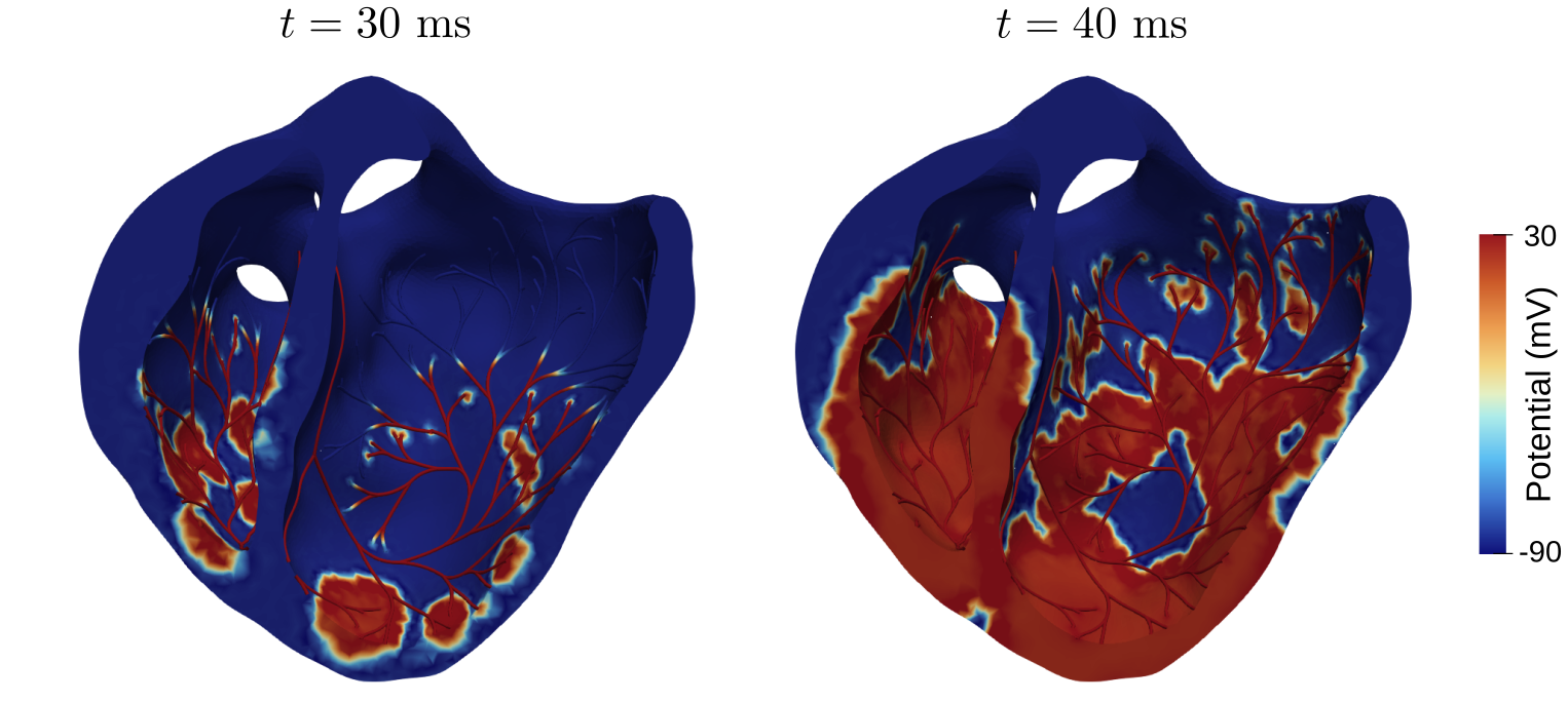
Cardiac electrophysiology simulation
Next, we evaluate the computational performance of svMultiPhysics for this cardiac electrophysiology case. In contrast to the AAA CFD and FSI examples, this problem involves the solution of a reaction–diffusion type system in a complex biventricular geometry coupled to a distributed Purkinje network. This example demonstrates that svMultiPhysics is not limited to fluid and solid mechanics applications, but also supports large-scale simulations of cardiac electrical activation within the same computational framework.
For the performance study, we report the total wall-clock time after completion of 500 time steps, corresponding to 50 ms of simulated time with a time step size of ms. Strong scalability is assessed by doubling the number of MPI processes starting from 4 processors, and the speedup is normalized by the wall-clock time measured for 500 steps on 4 processors. All simulations were performed using the same electrophysiology model, fiber architecture, Purkinje network, and stimulation protocol described above.
Fig 8 shows the strong scalability behavior for the electrophysiology simulation. The results indicate how efficiently the solver handles the repeated solution of the diffusion problem together with the ionic update over hundreds of time steps in an anatomically realistic biventricular model. Fig 9 presents the corresponding wall-clock times after 500 time steps. Across all processor counts, the in-house CG solver with diagonal preconditioning consistently yields the lowest wall-clock time, indicating its computational efficiency for this electrophysiology workload. Among the Trilinos-based approaches, the diagonal and RILUK(0) preconditioners provide competitive performance, while the multilevel (ML) preconditioner incurs higher computational cost, particularly at larger processor counts. When directly comparing identical solver–preconditioner combinations, namely GMRES with diagonal preconditioning, the Trilinos implementation achieves slightly lower wall-clock times than the in-house counterpart. This suggests that the optimized linear algebra kernels and data structures within the Trilinos library provide measurable performance benefits, even when using equivalent numerical algorithms. Overall, these results highlight both the efficiency of lightweight in-house solvers for this class of problems and the robustness of Trilinos-based implementations for scalable large-scale simulations.
Together, these results provide a representative measure of the computational cost of cardiac electrophysiology simulations in svMultiPhysics and complement the CFD and FSI performance studies presented earlier. The results also confirm the ability of svMultiPhysics to handle anatomically informed conductivity tensors, physiologically motivated Purkinje activation pathways, and realistic ventricular-scale electrophysiology simulations within a unified finite element solver framework.


Conclusions
In this work, we presented svMultiPhysics, an open-source, MPI-parallel finite element solver designed for cardiovascular applications and built to support tightly coupled multiphysics simulations. The solver is implemented in modern C++ and provides a unified computational framework in which the governing equations of fluid dynamics, solid mechanics, scalar transport, and cardiac electrophysiology can be solved either independently or in strongly coupled configurations. This integrated design represents one of the core strengths of svMultiPhysics, enabling researchers to investigate complex physiological interactions within a consistent numerical and data-structural environment. Although the present work focuses primarily on solver capabilities and computational performance, confidence in the accuracy of svMultiPhysics is supported by a broader validation history of the SimVascular solver ecosystem and its precursor formulations. Published validation studies have demonstrated strong agreement between computational predictions and experimental or in vivo measurements across several cardiovascular applications, including patient-specific coronary aneurysm hemodynamics in Kawasaki disease, vascular fluid–structure interaction against in vitro 4D-flow MRI, pressure-drop estimation in aortic coarctation, and heart-valve hemodynamics against in vitro 4D-flow MRI data [99, 100, 101, 102].
A key component of the solver is its flexible linear algebra interface. svMultiPhysics incorporates an in-house linear solver suite and provides seamless interoperability with two major scientific libraries, PETSc and Trilinos. This approach offers users a broad spectrum of linear solvers and preconditioners, allowing the selection of methods best suited to the problem being solved. Such flexibility is fundamental for tackling the large, non-linear, coupled, and often ill-conditioned systems that arise in cardiovascular simulations.
To illustrate the solver’s capabilities, we considered three representative applications, a CFD and an FSI simulation of a patient-specific abdominal aortic aneurysm; and a cardiac electrophysiology simulation ona patient-specific biventricular geometry with CHD. These examples highlight the ability of svMultiPhysics to handle realistic geometries, non-linear multiphysics coupling, and large-scale parallel execution. The strong scalability study demonstrates excellent parallel performance up to 256 processes for both CFD and FSI cases, underscoring the suitability of the solver for high-performance computing environments. The wall-clock time comparison across different linear solvers and preconditioners further illustrates the flexibility and efficiency of the available solution strategies.
Preliminary CPU-GPU comparisons show the significant potential of Kokkos-enabled Trilinos backend for accelerating large-scale simulations. By shifting Krylov solvers and preconditioner operations on the GPU, the AAA CFD case achieved up to approximately reduction in wall-clock time for the Trilinos diagonal preconditioner and approximately – reductions for the ML preconditioner. These results highlight the promise of heterogeneous architectures in advancing multiphysics cardiovascular simulations.
The current C++ implementation of svMultiPhysics originates from a systematic translation of the previous Fortran-based solver svFSI [30]. Ongoing development efforts are focused on achieving a fully object-oriented design to improve modularity, maintainability, and extensibility. This refactoring will ensure that new physics modules, numerical strategies, and solver components can be incorporated with minimal friction, supporting the long-term sustainability and evolution of the project.
As the multiphysics backend of the SimVascular project, svMultiPhysics provides the foundation for advanced cardiovascular modeling workflows. By documenting its governing equations, numerical formulations, code architecture, and representative applications, this paper aims to serve both users and developers. Our goal is to provide a clear and comprehensive reference that supports reproducibility, encourages community contributions, and fosters the continued growth of an open-source platform for cardiovascular simulation research.
svMultiPhysics is actively maintained, extensively documented, and openly developed on GitHub, ensuring transparency and long-term sustainability. Its unified multiphysics capabilities, coupled with robust parallel performance, position it as a versatile tool for investigating complex cardiovascular problems—from fundamental biomechanical studies to clinical applications.
Supporting information
S1 Appendix
Constitutive material models implemented in svMultiPhysics.
S2 website
https://github.com/SimVascular/svMultiPhysics The GitHub repository for svMultiPhysics.
S3 website
https://github.com/SimVascular/svZeroDSolver The GitHub repository for svZeroDSolver.
S4 website
https://hub.docker.com/u/simvascular The SimVascular DockerHub page contains images of pre–built svMultiPhysics and all necessary libraries.
S5 website
https://simvascular.github.io The SimVascular website contains an extensive documentation on the svMultiPhysics solver.
Data Availability
Data availability. The svMultiPhysics source code is openly available from the SimVascular GitHub repository at https://github.com/SimVascular/svMultiPhysics.git. The solver is maintained as a core module of the SimVascular open-source framework, available at https://github.com/SimVascular. Documentation for SimVascular and its components is available at https://simvascular.github.io/. Example problems and testing cases are included in the svMultiPhysics repository. Additional cardiovascular models suitable for simulation are available through the Vascular Model Repository (VMR) database at https://www.vascularmodel.com/. Simulation data generated for this study are available from the corresponding author upon reasonable request.
Acknowledgments
This work was supported by the National Science Foundation under award number 2310909. We acknowledge the computational resources and technical support provided by the Stanford Research Computing Center and the Texas Advanced Computing Center, which enabled the simulations and performance studies presented in this work.
References
- 1. Sun Z. Advances in Cardiovascular Imaging: A Platform to Share Recent Research Findings Through Utilization of Advanced Imaging Technologies. J Cardiovasc Dev Dis. 2025;12(10):382. doi:10.3390/jcdd12100382.
- 2. Vardhan M, Randles A. Application of physics-based flow models in cardiovascular medicine: Current practices and challenges. Biophys Rev (Melville). 2021;2(1):011302. doi:10.1063/5.0040315.
- 3. Schwarz EL, Pegolotti L, Pfaller MR, Marsden AL. Beyond CFD: Emerging methodologies for predictive simulation in cardiovascular health and disease. Biophys Rev. 2023;4(1). doi:10.1063/5.0109400.
- 4. Hrvoje J. OpenFOAM: Open source CFD in research and industry. Int J Nav Archit Ocean Eng. 2009;1(2):89–94. doi:10.2478/IJNAOE-2013-0011.
- 5. Maas SA, Ellis BJ, Ateshian GA, Weiss JA. FEBio: Finite Elements for Biomechanics. ASME J Biomech Eng. 2012;134(1):011005. doi:10.1115/1.4005694.
- 6. Alnæs MS, Logg A, Ølgaard KB, Rognes ME, Wells GN. Unified form language: A domain-specific language for weak formulations of partial differential equations. ACM Trans Math Softw. 2014;40(2). doi:10.1145/2566630.
- 7. Arndt D, Bangerth W, Davydov D, Heister T, Heltai L, Kronbichler M, Maier M, Pelteret J–P, Turcksin B, Wells D. The deal.II finite element library: Design, features, and insights. Comput Math Appl. 2021;81:407–422. doi:10.1016/j.camwa.2020.02.022.
- 8. Arndt D, Bangerth W, Bergbauer M, Blais B, Fehling M, Gassmöller R, Heister T, Heltai L, Kronbichler M, Maier M, Munch P. The deal.II library, version 9.7. J Numer Math. 2025;33(4):403–415. doi:10.1515/jnma-2024-0094.
- 9. Pitt-Francis J, Pathmanathan P, Bernabeu MO, Bordas R, Cooper J, Fletcher AG, Mirams GR, Murray P, Osborne JM, Walter A, Chapman SJ, Garny A, van Leeuwen IMM, Maini PK, Rodríguez B, Waters SL, Whiteley JP, Byrne HM, Gavaghan DJ. Chaste: A test-driven approach to software development for biological modelling. Computer Physics Communications. 2009;180(12):2452–2471. doi:10.1016/j.cpc.2009.07.019.
- 10. Africa PC. lifex: A flexible, high performance library for the numerical solution of complex finite element problems. SoftwareX. 2022;20:101252. doi:10.1016/j.softx.2022.101252.
- 11. Bucelli M. The lifex library version 2.0. ACM Trans Math Softw. 2025;51(4):1–10. doi:10.1145/3759530.
- 12. Africa PC, Piersanti R, Regazzoni F, Bucelli M, Salvador M, Fedele M, Pagani S, Dede’ L, Quarteroni A. lifex-ep: a robust and efficient software for cardiac electrophysiology simulations. BMC Bioinformatics. 2023;24(1):389. doi:10.1186/s12859-023-05513-8.
- 13. Fedele M, Piersanti R, Regazzoni F, Salvador M, Africa P–C, Bucelli M, Zingaro A, Quarteroni A. A comprehensive and biophysically detailed computational model of the whole human heart electromechanics. Comput Methods Appl Mech Eng. 2023;410:115983. doi:10.1016/j.cma.2023.115983.
- 14. Africa PC, Fumagalli I, Bucelli M, Zingaro A, Fedele M, Dede’ L, Quarteroni A. lifex-cfd: An open-source computational fluid dynamics solver for cardiovascular applications. Computer Physics Communications. 2024;296:109039. doi:10.1016/j.cpc.2023.109039.
- 15. Lee J, Cookson A, Roy I, Kerfoot E, Asner L, Vigueras G, Sochi T, Deparis S, Michler C, Smith NP, Nordsletten DA. Multiphysics Computational Modeling in . SIAM Journal on Scientific Computing. 2016;38(3):150–178. doi:10.1137/15M1014097.
- 16. 4C. 4C: A Comprehensive Multiphysics Simulation Framework. https://www.4c-multiphysics.org. Accessed: November 17, 2025.
- 17. Plank G, Loewe A, Neic A, Augustin C, Huang Y–L, Gsell MAF, Karabelas E, Nothstein M, Prassl AJ, Sanchez J, Seemann G, Vigmond EJ. The openCARP simulation environment for cardiac electrophysiology. Comput Methods Programs Biomed. 2021;208:106223. doi:10.1016/j.cmpb.2021.106223.
- 18. Zhou B, Balmus M, Corrado C, Cicci L, Qian S, Niederer S–A. TorchCor: High-performance cardiac electrophysiology simulations with the finite element method on GPUs. SoftwareX. 2026;33:102521. doi:10.1016/j.softx.2025.102521.
- 19. Garny A, Hunter PJ. OpenCOR: a modular and interoperable approach to computational biology. Front Physiol. 2015;6:26. doi:10.3389/fphys.2015.00026.
- 20. Kjeldsberg H–A, Sundnes J, Valen–Sendstad K. A verified and validated moving domain computational fluid dynamics solver with applications to cardiovascular flows. Int J Numer Methods Biomed Eng. 2023;39(6):e3703. doi:10.1002/cnm.3703.
- 21. Arthurs CJ, Khlebnikov R, Melville A, Marčan M, Gomez A, Dillon-Murphy D, Cuomo F, Silva Vieira M, Schollenberger J, Lynch SR, Tossas-Betancourt C. CRIMSON: An open-source software framework for cardiovascular integrated modelling and simulation. PLOS Computational Biology 17(5): e1008881. https://doi.org/10.1371/journal.pcbi.1008881
- 22. Griffith BE. IBAMR: Immersed boundary adaptive mesh refinement. 2017.
- 23. Vázquez M, Houzeaux G, Koric S, Artigues A, Aguado–Sierra J, Arís R, Mira D, Calmet H, Cucchietti F, Owen H, Taha A, Burness E, Cela JM, Valero M. Alya: Multiphysics engineering simulation toward exascale. J Comput Sci. 2016;14:15–27. doi:10.1016/j.jocs.2015.12.007.
- 24. Santiago A, Aguado–Sierra J, Zavala–Aké M, Doste R, Gómez S, Arís R, Cajas JC, Casoni E, Vázquez M. Fully coupled fluid-electro-mechanical model of the human heart for supercomputers. Int J Numer Methods Biomed Eng. 2018;34(12):e3140. doi:10.1002/cnm.3140.
- 25. Balay S, Abhyankar S, Adams MF, Benson S, Brown J, Brune P, Buschelman K, Constantinescu EM, Dalcin L, Dener A, Eijkhout V, Faibussowitsch J, Gropp WD, Hapla V, Isaac T, Jolivet P, Karpeev D, Kaushik D, Knepley MG, Kong F, Kruger S, May DA, McInnes LC, Mills RT, Mitchell L, Munson T, Roman JE, Rupp K, Sanan P, Sarich J, Smith BF, Zampini S, Zhang H, Zhang H, Zhang J. PETSc Web page. https://petsc.org/.
- 26. The Trilinos Project Team. The Trilinos Project Website. https://trilinos.github.io. Accessed May 22, 2020).
- 27. Updegrove A, Wilson NM, Merkow J, Lan H, Marsden AL, Shadden SC. SimVascular: An Open Source Pipeline for Cardiovascular Simulation. Ann Biomed Eng. 2017;45:525–541. doi:10.1007/s10439-016-1762-8.
- 28. Trott C, Lebrun-Grandié D, Arndt D, Ciesko J, Dang V, Ellingwood N, Gayatri R, Harvey E, Hollman DS, Ibanez D, and others. Kokkos 3: Programming model extensions for the exascale era IEEE Transactions on Parallel and Distributed Systems. 2021 Jul 14;33(4):805-17. doi:10.1109/TPDS.2021.3097283
- 29. Mayr M, Heinlein A, Glusa C, Rajamanickam S, Arnst M, Bartlett R, Berger-Vergiat L, Boman E, Devine K, Harper G, and others. Trilinos: enabling scientific computing across diverse hardware architectures at scale. 2025 arXiv preprint arXiv:2503.08126
- 30. Zhu C, Vedula V, Parker D, Wilson N, Shadden SC, Marsden AL. svFSI: A Multiphysics Package for Integrated Cardiac Modeling. Journal of Open Source Software. 2022;7(78):4118. doi:10.21105/joss.04118.
- 31. Rahn AW, Tien C, Cerny LC. Flow properties of blood under low shear rate. In: Hershey D, editor. Chemical Engineering in Medicine and Biology. Boston: Springer US; 1967. p. 45–83.
- 32. Chandran KB, Rittgers SE, Yoganathan AP. Biofluid mechanics: the human circulation. 1st ed. Boca Raton: CRC Press; 2006.
- 33. Boyd J, Buick JM, Green S. Analysis of the Casson and Carreau–Yasuda non-Newtonian blood models in steady and oscillatory flows using the lattice Boltzmann method. Phys Fluids. 2007;19(9):093103. doi:10.1063/1.2772250.
- 34. Hughes TJR, Mazzei L, Jansen K. Large eddy simulation and the variational multiscale method. Comput Visual Sci. 2000;3:47–59. doi:10.1007/s007910050051.
- 35. Bazilevs Y, Calo VM, Cottrell JA, Hughes TJR, Reali A, Scovazzi G. Variational multiscale residual-based turbulence modeling for large eddy simulation of incompressible flows. Comput Methods Appl Mech Eng. 2007;197(1–4):173–201. doi:10.1016/j.cma.2007.07.016.
- 36. Gerosa FM, Marsden AL. A mechanically consistent unified formulation for fluid–porous–structure–contact interaction. Comput Methods Appl Mech Eng. 2024;425:116942.
- 37. Fuchsberger J, Aigner P, Niederer S, Plank G, Schima H, Haase G, Karabelas E. On the incorporation of obstacles in a fluid flow problem using a Navier–Stokes–Brinkman penalization approach. J Comput Sci. 2022 Jan;57:101506.
- 38. Astorino M, Hamers J, Shadden SC, Gerbeau JF. A robust and efficient valve model based on resistive immersed surfaces Int J Numer Meth Biomed Eng. 2012;28(9):937-959. https://doi.org/10.1002/cnm.2474.
- 39. Fedele M, Faggiano E, Dedé L, Quarteroni A. A patient-specific aortic valve model based on moving resistive immersed implicit surfaces. Biomech Model Mechanobiol. 2017;16:1779–1803. https://doi.org/10.1007/s10237-017-0919-1.
- 40. This A, Boilevin‐Kayl L, Fernández MA, Gerbeau JF. Augmented resistive immersed surfaces valve model for the simulation of cardiac hemodynamics with isovolumetric phases. Int J Numer Meth Biomed Eng. 2020;36(3),e3223. https://doi.org/10.1002/cnm.3223.
- 41. Bucelli M, Zingaro A, Africa PC, Fumagalli I, Dedé L, Quarteroni A. A mathematical model that integrates cardiac electrophysiology, mechanics, and fluid dynamics: Application to the human left heart. Int J Numer Meth Biomed Eng. 2023;39(3):e3678. https://doi.org/10.1002/cnm.3678.
- 42. Zhao H, Kaiser AD, Kong F, Brown AL, Hu Z, Codoni D, Dave S, Marsden AL. Comparative analysis of resistive immersed surface and immersed boundary methods for aortic valve simulation. arXiv preprint arXiv:2607.01662. 2026.
- 43. Fung YC. Biomechanics: Mechanical Properties of Living Tissues. 2nd ed. New York: Springer–Verlag; 1993.
- 44. Holzapfel GA. Nonlinear solid mechanics: a continuum approach for engineering science. Wiley; 2002
- 45. Simo JC, Taylor RL. Quasi-incompressible finite elasticity in principal stretches. continuum basis and numerical algorithms. Comput Methods Appl Mech Eng. 1991;85(3), 273–310 doi:10.1016/0045-7825(91)90100-K.
- 46. Miehe C. Aspects of the formulation and finite element implementation of large strain isotropic elasticity. Int. J. Numer. Methods Eng. 1994;37(12), 1981–2004 doi:10.1002/nme.1620371202.
- 47. Gasser TC, Ogden RW, Holzapfel GA. Hyperelastic modelling of arterial layers with distributed collagen fibre orientations. J R Soc Interface. 2006;3:15–35. doi:10.1098/rsif.2005.0073.
- 48. Ortiz M, Stainier L. The variational formulation of viscoplastic constitutive updates. Comput Methods Appl Mech Eng. 1999;171(3), 419-444 10.1016/S0045-7825(98)00219-9.
- 49. Guccione JM, McCulloch AD, Waldman LK. Passive material properties of intact ventricular myocardium determined from a cylindrical model. J Biomech Eng. 1991;113(1):42–55. doi:10.1115/1.2894084.
- 50. Chapelle D, Le Tallec P, Moireau P, Sorine M. Energy-Preserving Muscle Tissue Model: Formulation and Compatible Discretizations. Int J Multiscale Comput Eng. 2012;10(2), 189-211 10.1615/IntJMultCompEng.2011002360.
- 51. Holzapfel GA, Ogden RW. Constitutive modelling of passive myocardium: a structurally based framework for material characterization. Phil Trans R Soc A. 2009;367:3445–3475. doi:10.1098/rsta.2009.0091.
- 52. Nolan DR, Gower AL, Destrade M, Ogden RW, McGarry JP. A robust anisotropic hyperelastic formulation for the modelling of soft tissue. J Mech Behav Biomed Mater 2014;39, 48-60 doi:10.1016/j.jmbbm.2014.06.016.
- 53. Shi L, Chen IY, Takayama H, Vedula V. An optimization framework to personalize passive cardiac mechanics. Comput Methods Appl Mech Eng. 2024;432(Pt A):117401. doi:10.1016/j.cma.2024.117401.
- 54. Peirlinck, M., Hurtado, J.A., Rausch, M.K. et al. A universal material model subroutine for soft matter systems. Engineering with Computers. 41, 905–927 (2025). doi:https://doi.org/10.1007/s00366-024-02031-w.
- 55. Bayer JD, Blake RC, Plank G, Trayanova, NA. A Novel Rule-Based Algorithm for Assigning Myocardial Fiber Orientation to Computational Heart Models. Ann Biomed Eng. 2012;40(10):2243–2254. doi:10.1007/s10439-012-0593-5.
- 56. Liu J, Marsden AL. A unified continuum and variational multiscale formulation for fluids, solids, and fluid–structure interaction. Comput Methods Appl Mech Eng. 2018;337:549–597. doi:10.1016/j.cma.2018.03.045.
- 57. Esmaily-Moghadam M, Hsia T–Y, Marsden AL. A non-discrete method for computation of residence time in fluid mechanics simulations. Phys Fluids. 2013;25(11):110802. doi:10.1063/1.4819142.
- 58. ten Tusscher KHWJ, Panfilov AV. Alternans and spiral breakup in a human ventricular tissue model. Am J Physiol Heart Circ Physiol. 2006;291(3):H1088–H1100. doi:10.1152/ajpheart.00109.2006.
- 59. Göktepe S, Kuhl E. Computational modeling of cardiac electrophysiology: a novel finite element approach. Int J Numer Meth Eng. 2009;79:156–178. doi:10.1002/nme.2571.
- 60. Bueno-Orovio A, Cherry EM, Fenton FH. Minimal model for human ventricular action potentials in tissue. J Theor Biol. 2008;253(3):544–560. doi:10.1016/j.jtbi.2008.03.029.
- 61. Salvador M, Marsden AL. Branched latent neural maps. Comput Methods Appl Mech Eng. 2024;418:116499. doi:10.1016/j.cma.2023.116499.
- 62. Hughes TJR. The finite element method: linear static and dynamic finite element analysis. Prentice-Hall, Englewood Cliffs, NJ. 1987.
- 63. Tabata M. A finite element approximation corresponding to the upwind finite differencing. Memoirs of Numerical Mathematics. 1977;4:47–63.
- 64. Hughes TJR, Tezduyar TE. Finite element methods for first-order hyperbolic systems with particular emphasis on the compressible Euler equations. Comput Methods Appl Mech Eng. 1984;45(1):217–284. doi:10.1016/0045-7825(84)90157-9.
- 65. Brooks AN, Hughes TJR. Streamline upwind/Petrov-Galerkin formulations for convection dominated flows with particular emphasis on the incompressible Navier-Stokes equations. Comput Methods Appl Mech Eng. 1982;32(1):199–259. doi:10.1016/0045-7825(82)90071-8.
- 66. Marsden AL. Multiscale modeling of cardiovascular flows for clinical decision support. Appl Mech Rev. 2015;67(3):030804. doi:10.1115/1.4027343.
- 67. Jansen KE, Whiting CH, Hulbert GM. A generalized- method for integrating the filtered Navier–Stokes equations with a stabilized finite element method. Comput Methods Appl Mech Eng. 2000;190(3–4):305–319. doi:10.1016/S0045-7825(00)00203-6.
- 68. Whiting CH, Jansen KE. A stabilized finite element method for the incompressible Navier–Stokes equations using a hierarchical basis. Int J Numer Meth Fluids. 2001;35:93–116. doi:10.1002/1097-0363(20010115)35:1¡93::AID-FLD85¿3.0.CO;2-G
- 69. Chung J, Hulbert GM. A Time Integration Algorithm for Structural Dynamics With Improved Numerical Dissipation: The Generalized- method. ASME J Appl Mech. 1993;60(2):371–375. doi:10.1115/1.2900803
- 70. Esmaily Moghadam M, Vignon-Clementel IE, Figliola R, Marsden AL. A modular numerical method for implicit 0D/3D coupling in cardiovascular finite element simulations. J Comput Phys. 2013;244:63–79. doi:10.1016/j.jcp.2012.07.035.
- 71. Brown AL, Salvador M, Shi L, Pfaller MR, Hu Z, Harold KE, Hsiai T, Vedula V, Marsden AL. A modular framework for implicit 3D–0D coupling in cardiac mechanics. Comput Methods Appl Mech Eng. 2024;421:116764. doi:10.1016/j.cma.2024.116764.
- 72. Esmaily-Moghadam M, Bazilevs Y, Marsden AL. A new preconditioning technique for implicitly coupled multidomain simulations with applications to hemodynamics. Comput Mech. 2013;52(5):1141–1152. doi:10.1007/s00466-013-0868-1.
- 73. Kung E, Baretta A, Baker C, Arbia G, Biglino G, Corsini C, Schievano S, Vignon-Clementel IE, Dubini G, Pennati G, Taylor A, Dorfman A, Hlavacek AM, Marsden AL, Hsia T-Y, Migliavacca F. Predictive modeling of the virtual Hemi-Fontan operation for second stage single ventricle palliation: Two patient-specific cases. J. Biomech. 2013;46(2):423–429. doi:10.1016/j.jbiomech.2012.10.023.
- 74. Seo J, Fleeter C, Kahn AM, Marsden AL, Schiavazzi DE. Multifidelity estimators for coronary circulation models under clinically informed data uncertainty. Int J Uncertain Quantif. 2020;10(5):449-466. doi:10.1615/int.j.uncertaintyquantification.2020033068.
- 75. Arthurs CJ, Xiao N, Moireau P, Schaeffter T, Figueroa CA. A flexible framework for sequential estimation of model parameters in computational hemodynamics. Adv Model and Simul in Eng Sci. 2020;7(48). doi:10.1186/s40323-020-00186-x.
- 76. Vignon–Clementel IE, Figueroa CA, Jansen KE, Taylor CA. Outflow boundary conditions for 3D simulations of non–periodic blood flow and pressure fields in deformable arteries. Computer Methods in Biomechanics and Biomedical Engineering. 2010;3(5):625–640. doi:10.1080/10255840903413565.
- 77. Vignon–Clementel IE, Figueroa CA, Jansen KE, Taylor CA. Outflow boundary conditions for three-dimensional finite element modeling of blood flow and pressure in arteries. Computer methods in applied mechanics and engineering. 2006 Jun 1;195(29-32):3776-96.
- 78. Esmaily-Moghadam M, Bazilevs Y, Marsden AL. A bi-partitioned iterative algorithm for solving linear systems arising from incompressible flow problems. Comput Methods Appl Mech Eng. 2015;286:40–62. doi:10.1016/j.cma.2014.11.033.
- 79. Esmaily–Moghadam M, Bazilevs Y, Marsden AL. A new preconditioning technique for implicitly coupled multidomain simulations with applications to hemodynamics. Comput Mech. 2013;52:1141–1152. doi:10.1007/s00466-013-0868-1.
- 80. Baker CG, Heroux MA. Tpetra, and the use of generic programming in scientific computing Scientific Programming. 2012;20(2):115-28. doi:10.3233/SPR-2012-0349
- 81. Hughes TJR, Kam Liu W, Zimmermann TK. Lagrangian-Eulerian finite element formulation for incompressible viscous flows. Comput Methods Appl Mech Eng. 1981; 29(3):329–349. doi:10.1016/0045-7825(81)90049-9.
- 82. Bazilevs Y, Hsu MC, Takizawa K, Tezduyar TE. ALE–VMS and ST–VMS methods for computer modeling of wind turbine rotor aerodynamics and fluid–structure interaction. Mathematical Models and Methods in Applied Sciences. 2012; 22(SUPPL.2). doi:10.1142/S0218202512300025.
- 83. Figueroa CA, Vignon-Clementel IE, Jansen KE, Hughes TJR, Taylor CA. A coupled momentum method for modeling blood flow in three–dimensional deformable arteries. Comput Methods Appl Mech Eng. 2006;195(41–43):5685–5706. doi:10.1016/j.cma.2005.11.011.
- 84. Schroeder W, Martin K, Lorensen B. The Visualization Toolkit. 4th ed. Kitware; 2006. ISBN: 978-1-930934-19-1.
- 85. Ortiz AK, Aleiou AA, LaDisa JF, Wilson NM, Stanford University, Vascular Model Repository, Open Source Medical Software Corporation (OSMSC). 0031_H_ABAO_AAA. Stanford Digital Repository. 2025.
- 86. Si H. Adaptive tetrahedral mesh generation by constrained Delaunay refinement. Int J Numer Methods Eng. 2008;75(7):856–880. doi:10.1002/nme.2318.
- 87. Sullivan B, Kaszynski A. PyVista: 3D plotting and mesh analysis through a streamlined interface for the Visualization Toolkit (VTK). Journal of Open Source Software. 2019;4(37):1450. doi:10.21105/joss.01450.
- 88. Bäumler K, Vedula V, Sailer AM, Seo J, Chiu P, Mistelbauer G, Chan FP, Fischbein MP, Marsden AL, Fleischmann D. Fluid–structure interaction simulations of patient–specific aortic dissection. Biomech Model Mechanobiol. 2020;19(5):1607–1628. doi:10.1007/s10237-020-01294-8.
- 89. Lan IS, Liu J, Yang W, Marsden AL. Numerical investigation of abdominal aortic aneurysm hemodynamics using the reduced unified continuum formulation for vascular fluid–structure interaction. Forces Mech. 2022;7:100089. doi:10.1016/j.finmec.2022.100089.
- 90. Pfaller MR, Pham J, Wilson NM, Parker DW, Marsden AL. On the periodicity of cardiovascular fluid dynamics simulations. Ann Biomed Eng. 2021;49(12):3574–3592. doi:10.1007/s10439-021-02796-x.
- 91. Maher GD, Fleeter CM, Schiavazzi DE, Marsden AL. Geometric uncertainty in patient-specific cardiovascular modeling with convolutional dropout networks. Comput Methods Appl Mech Eng. 2021;386:114038. doi:10.1016/j.cma.2021.114038.
- 92. Kaiser AD, Shad R, Hiesinger W, Marsden AL. A design–based model of the aortic valve for fluid–structure interaction. Biomech Model Mechanobiol. 2021;20(6):2413–2435. doi:10.1007/s10237-021-01516-7.
- 93. Moireau P, Xiao N, Astorino M, Figueroa CA, Chapelle D, Taylor CA, Gerbeau JF. External tissue support and fluid-structure simulation in blood flows. Biomech Model Mechanobiol. 2012;11(1–2):1–18. doi:10.1007/s10237-011-0289-z.
- 94. Liu J, Yang W, Dong M, Marsden AL. The nested block preconditioning technique for the incompressible Navier–Stokes equations with emphasis on hemodynamic simulations. Comput Methods Appl Mech Eng. 2020;367:113122. doi:10.1016/j.cma.2020.113122.
- 95. Seo J, Schiavazzi DE, Marsden AL. Performance of preconditioned iterative linear solvers for cardiovascular simulations in rigid and deformable vessels. Comput Mech. 2019;64(3):717–739. doi:10.1007/s00466-019-01678-3.
- 96. Doste R, Soto-Iglesias D, Bernardino G, Alcaine A, Sebastian R, Giffard-Roisin S, Sermesant M, Berruezo A, Sanchez-Quintana D, Camara O. A rule-based method to model myocardial fiber orientation in cardiac biventricular geometries with outflow tracts. Int J Numer Meth Biomed Eng. 2019;35(4). doi:10.1002/cnm.3185.
- 97. Sahli Costabal F, Hurtado DE, Kuhl E. Generating Purkinje networks in the human heart. J Biomech. 2016;49(12):2455–2465. doi:10.1016/j.jbiomech.2015.12.025.
- 98. ten Tusscher KHWJ, Noble D, Noble PJ, Panfilov AV. A model for human ventricular tissue. Am J Physiol Heart Circ Physiol. 2004;286(4):H1573–H1589. doi:10.1152/ajpheart.00794.2003.
- 99. Kung E, Kahn AM, Burns JC, Marsden A. In vitro validation of patient-specific hemodynamic simulations in coronary aneurysms caused by Kawasaki disease. Cardiovasc Eng Technol. 2014;5(2):189–201. doi:10.1007/s13239-014-0184-8.
- 100. Lan IS, Liu J, Yang W, Zimmermann J, Ennis DB, Marsden AL. Validation of the reduced unified continuum formulation against in vitro 4D-flow MRI. Ann Biomed Eng. 2023;51(2):377–393. doi:10.1007/s10439-022-03038-4.
- 101. Nair PJ, Pfaller MR, Dual SA, McElhinney DB, Ennis DB, Marsden AL. Non-invasive estimation of pressure drop across aortic coarctations: validation of 0D and 3D computational models with in vivo measurements. Ann Biomed Eng. 2024;52(5):1335–1346. doi:10.1007/s10439-024-03457-5.
- 102. Seresti A, Marsden AL, Kahn AM, Reeves RR, Mahmud E, Al Khiami B, Ang L, Khan MO. Validation of CTA-based closed-loop coronary artery flow simulations against intravascular Doppler velocity and pressure measurements. Comput Methods Programs Biomed. 2025;268:108868. doi:10.1016/j.cmpb.2025.108868.