

DAUPNet: Domain-Aware Uncertainty Modeling for Reliable Prototype Discrimination in Cross-Domain Few-Shot Semantic Segmentation
Abstract
Cross-domain few-shot semantic segmentation (CD-FSS) has predominantly been formulated as learning domain-invariant representations or improving support-query correspondence. Nevertheless, large domain shifts still make prototype matching unreliable: inconsistent hierarchical responses corrupt the support representation, deterministic prototypes cannot express boundary and appearance ambiguity, and treating prototypes with different reliability equally during optimization weakens foreground-background separation. We therefore propose DAUPNet, a unified framework that reformulates cross-domain prototype matching as uncertainty-aware prototype discrimination. DAUPNet first harmonizes hierarchical support-query features to provide stable evidence, then represents foreground and background prototypes probabilistically, and finally uses their estimated uncertainty to regulate contrastive optimization. On four standard target domains, DAUPNet achieves 72.6% and 76.7% average mIoU in the 1-shot and 5-shot settings, respectively, including substantial gains on the two medical domains. These results demonstrate that modeling prototype uncertainty and incorporating it into optimization provides a robust and interpretable approach to CD-FSS under severe domain shift. The code is available at https://github.com/madness-Lei/DAUPNet.
Introduction

Few-shot semantic segmentation (FSS) segments novel classes from only a few annotated support images, reducing the dependence of conventional segmentation models on dense annotations and fixed training categories. In practical applications, however, support and query images may come from domains that differ markedly from the source training data in acquisition modality, texture, contrast, and object structure. Cross-domain few-shot semantic segmentation (CD-FSS) addresses this setting, but the combined scarcity of annotations and domain shift makes reliable support-query transfer particularly difficult. Existing studies have approached this difficulty through domain-invariant representation (Lei et al. 2022), target-domain adaptation and support-query correspondence mining (Nie et al. 2024; Su et al. 2024) , and multi-scale or low-level feature enhancement (Tong et al. 2024; Liu et al. 2025; Sun et al. 2026). Despite this progress, segmentation remains fragile when domain shift undermines the reliability of the prototypes on which support-query matching depends.
This prototype-reliability problem extends beyond feature alignment and arises throughout prototype construction and discrimination. First, separately processing high-level semantics and low-level appearance leaves cross-level evidence inconsistent, so the representation pooled into a prototype may already be unstable. Second, masked average pooling compresses that evidence into a deterministic vector and therefore cannot indicate whether the support region has an ambiguous boundary, weak contrast, or heterogeneous appearance. Third, conventional contrastive optimization treats prototype combinations with different uncertainty as equally reliable, allowing unstable comparisons to disproportionately shape the foreground-background decision boundary. These effects are coupled: misaligned features produce uncertain prototypes, and optimizing them without accounting for their reliability further amplifies unstable discrimination.
Fig.1 contrasts conventional prototype matching with our uncertainty-aware formulation. A deterministic baseline pools the support foreground into a single vector and applies it to the query as if the underlying evidence were equally reliable across domains. DAUPNet instead preserves a reliability chain: hierarchical harmonization stabilizes the evidence used to form prototypes; probabilistic representation exposes residual foreground and background uncertainty; and variance-aware optimization reduces the influence of unreliable prototype comparisons on the decision margin.
Based on this view, we propose DAUPNet, a unified prototype learning framework organized around reliable uncertainty-aware discrimination rather than a collection of independent enhancements. DAUPNet retains the simplicity of prototype-based segmentation and implements the reliability chain in three successive stages. Hierarchical Domain-Aware Harmonization (HDH) coordinates multi-level support-query features so that prototype estimation starts from consistent cross-domain evidence. Probabilistic Prototype Representation (PPR) then models foreground and background as distributions, exposing uncertainty that a point prototype conceals. Finally, Variance-Aware Contrastive Learning (VACL) converts the variance-derived uncertainty into reliability weights, reducing the influence of unstable prototype comparisons while sharpening dependable foreground-background separation. Thus, each component supplies the prerequisite or supervision for the next, and all three serve the same objective: reliable prototype discrimination under domain shift.
Our main contributions are:
-
•
We identify unreliable prototype discrimination as a central bottleneck in CD-FSS and formulate its coupled causes across feature construction, uncertainty representation, and decision-margin optimization. This formulation provides a coherent alternative to treating domain shift solely as feature alignment.
-
•
We propose DAUPNet, which establishes an end-to-end reliability chain from hierarchical domain-aware harmonization to probabilistic foreground-background prototypes and variance-aware contrastive optimization. HDH stabilizes the evidence entering prototype estimation, while PPR and VACL expose and control the remaining uncertainty during representation and learning.
-
•
We show that uncertainty-aware prototype discrimination is especially valuable under severe appearance and modality shifts. DAUPNet improves the baseline by 6.9 mIoU on average in the 1-shot setting and reaches 72.6%/76.7% average mIoU across four target domains, with particularly strong performance on weak-boundary and grayscale medical images.

Related Work
Few-Shot Semantic Segmentations
FSS is primarily built upon prototype matching, dense correspondence modeling, and relational reasoning. PANet(Wang et al. 2019) establishes the foundational paradigm of masked average pooling and cosine matching. SSP(Fan et al. 2022) enhances representational capacity via query self-support prototypes(Peng et al. 2023). Subsequent work has improved discriminability through multi-prototype representation, cross-scale aggregation, and boundary enhancement. However, these deterministic prototypes assume stable feature distributions and clear boundaries—assumptions that break under domain shift. Overall, same-domain FSS has matured considerably. Yet most methods implicitly assume similar training-testing distributions. When significant modality discrepancies exist between source and target domains, their matching mechanisms often fail to maintain stable generalization performance (Min et al. 2021).
Cross-Domain Few-Shot Semantic Segmentation
CD-FSS simultaneously faces category scarcity and domain shift, making it a substantially harder yet more realistic extension.
Domain-Invariant Feature Learning. PATNet(Lei et al. 2022) pioneered the CD-FSS benchmark and proposed domain-invariant feature transformation. DMTN introduced dual matching for high-level semantics and low-level textures (Chen et al. 2024). However, these methods focus on feature alignment while neglecting prototype instability under domain shift.
Target-Domain Adaptation. IFA(Nie et al. 2024) improved adaptability by iteratively mining support-query correspondences. ABCDFSS(Herzog 2024) advocated test-time adaptation before comparison. Yet these iterative strategies still operate on deterministic prototypes that cannot capture cross-domain ambiguity.
Multi-Scale Enhancement. DR-Adapter(Su et al. 2024), APM(Tong et al. 2024), and LoEC(Liu et al. 2025) improve robustness via domain perturbation, frequency suppression, and low-level calibration. HSL(Sun et al. 2026) explore hierarchical semantics and state-space modeling (Cao et al. 2024)(Liu et al. 2026)(Lang et al. 2024)(Gao et al. 2026).
Despite this progress, existing approaches do not maintain prototype reliability throughout the complete matching pipeline: multi-scale evidence can remain inconsistent before pooling, deterministic prototypes hide ambiguity after pooling, and optimization does not account for unequal prototype uncertainty. DAUPNet addresses these coupled limitations through a single uncertainty-aware prototype discrimination framework.
Method
Problem Definition and Notation
This paper investigates CD-FSS. Let the source-domain training set be denoted as and the target-domain test or fine-tuning set as . The two domains have different image distributions, i.e., , and their training and testing categories are mutually disjoint. Each episode contains a support set and a query image. Under the 1-way -shot setting, the support set is defined as
| (1) |
where and denote the -th support image and its binary mask, respectively. The query image is denoted as . During training, the ground-truth query mask is available for computing the segmentation loss, whereas during inference only is given. The goal is to predict the query mask conditioned on .
Let denote the support or query branch, and let denote the feature level. The implementation uses , or when skip_layer4=True. The deepest layer is denoted as . After channel unification, each feature level has dimension , and the feature at level is written as
| (2) |
where denotes the batch size and denotes the spatial size.
Overall Framework
As shown in Fig.2 (a), DAUPNet realizes uncertainty-aware prototype discrimination as a sequential reliability chain comprising HDH, PPR, and VACL. The support image and query image are first fed into a shared encoder to extract multi-level features:
| (3) |
A Channel Reduce module projects features from different backbone stages into a unified feature space:
| (4) |
HDH then coordinates the support and query features across hierarchical levels and outputs harmonized features:
| (5) |
Based on the support harmonized features and the support mask, PPR estimates foreground and background probabilistic prototypes:
| (6) |
Here, denotes the prototype mean, while is a variance-derived estimate of prototype uncertainty. The foreground/background prototype means are matched with the deepest query feature to obtain a low-resolution prediction . The decoder then fuses this prediction with multi-level query features and progressively upsamples the result:
| (7) |
During training, the segmentation loss is computed using the query mask , and VACL uses the variance-derived uncertainty estimated by PPR to impose a reliability-weighted contrastive constraint on batch-level probabilistic prototypes. During inference, only prototype matching and decoding are performed, so the contrastive optimization introduces no additional inference branch.
Hierarchical Domain-Aware Harmonization Module
HDH is the first stage of the reliability chain. It reduces shallow texture noise, deep semantic compression, and support-query feature shift before prototype statistics are computed. Given the channel-reduced features and , HDH outputs harmonized features and . Rather than directly performing segmentation, HDH stabilizes the multi-level evidence from which PPR estimates prototype means and uncertainty.
As shown in Fig.2 (c), HDH follows a hierarchical coordination process consisting of intra-level processing, residual gating, bottom-up fusion, support-query channel recalibration, and top-down semantic feedback. Shallow levels focus on local texture and boundary information, while deeper levels emphasize structural semantics. A residual gate controls the balance between the original reduced feature and the intra-level refined feature:
| (8) |
The bottom-up path transfers boundary and texture information from shallower levels to deeper levels. For the current level , the preceding shallower output is downsampled to the same spatial size and denoted as . The fused feature is computed as
| (9) |
On the deepest level, Adaptive Channel Recalibration (ACR) estimates a shared channel weight from the support and query branches and applies it to both branches:
| (10) |
Finally, top-down refinement injects high-level semantic information into shallower levels:
| (11) |
Through these operations, HDH jointly improves boundary preservation, semantic consistency, and support-query alignment. The support features are used for probabilistic prototype estimation, the deepest query feature is used for prototype matching, and the multi-level query features are used by the decoder for spatial recovery.
Probabilistic Prototype Representation Module
As shown in Fig.2 (b), PPR is the second stage of the reliability chain. It converts the harmonized support evidence into probabilistic foreground/background prototypes through mask resizing, level-wise statistics, and fusion of the two deepest features. Unlike a deterministic prototype, each distribution retains both a class center and an explicit estimate of its uncertainty. Given the support HDH features and the support mask , the mask is first resized to each feature level, yielding . The background mask is defined as
| (12) |
The foreground and background pixel numbers are
| (13) |
where both values are clamped in the implementation to avoid division by zero. The foreground and background prototype means are computed as
| (14) |
To quantify the uncertainty concealed by a point prototype, PPR computes foreground and background feature variances:
| (15) | |||
A variance correction layer maps these dispersion statistics into nonnegative prototype uncertainty estimates:
| (16) | |||
When multiple feature levels are available, PPR fuses the deepest and second-deepest levels to balance semantic abstraction and spatial detail:
| (17) |
Variance fusion adopts a reciprocal weighting form:
| (18) | |||
Thus, PPR produces the foreground prototype and background prototype . The means are used for query matching, while both the means and their variance-derived uncertainty estimates are passed to VACL, connecting probabilistic representation directly to reliability-aware optimization. In the K-shot setting, prototypes are first extracted from each support sample and then averaged to obtain episode-level probabilistic prototypes.
Given the deepest query feature , prototype matching normalizes the query feature and prototype means:
| (19) | ||||
The foreground and background similarities are computed as
| (20) |
The low-resolution foreground probability is then obtained by softmax:
| (21) |
The decoder fuses with the multi-level query HDH features and upsamples the result to the original image size:
| (22) |
This design preserves the discriminative semantics of prototype matching while using shallow query features to recover spatial boundaries.
Variance-Aware Contrastive Learning Module

As shown in Fig.3, VACL completes the reliability chain by converting the variance-derived uncertainty from PPR into optimization weights. It collects batch-level foreground/background probabilistic prototypes, normalizes their representations, and constructs intra-class attraction and cross-class separation losses. Prototypes with lower estimated uncertainty contribute more strongly to class aggregation and foreground-background separation, whereas unreliable comparisons are prevented from dominating the decision margin (Khosla et al. 2020). Within a batch, foreground and background prototype means are concatenated as
| (23) | |||
with corresponding uncertainty estimates
| (24) | |||
The reliability weight of each prototype is generated from its average uncertainty:
| (25) |
After normalization, the cross-class similarity is computed as
| (26) |
The cross-class separation term is defined as
| (27) |
For intra-class attraction, VACL forms foreground-foreground and background-background prototype pairs within each batch. Pairs with lower similarity receive higher rank-based attention, summarized as
| (28) | |||
The final VACL loss is
| (29) |
If the batch contains no valid positive pairs, VACL returns a zero loss.
Loss Computation
During training, binary cross-entropy is used as the main segmentation loss:
| (30) |
The total loss combines segmentation supervision with the auxiliary VACL constraint:
| (31) |
Here, corresponds to ‘contrast_weight‘ in the implementation. enforces pixel-level consistency, while regularizes foreground/background relations according to variance-derived prototype uncertainty. VACL is used during training or fine-tuning but is disabled during inference.
| Method | Venue | Backbone | DeepGlobe | ISIC | Chest X-ray | FSS | Mean | |||||
| 1-shot | 5-shot | 1-shot | 5-shot | 1-shot | 5-shot | 1-shot | 5-shot | 1-shot | 5-shot | |||
| SSP | ECCV-22 | ResNet-50 | 40.0 | 48.7 | 35.5 | 45.9 | 74.4 | 74.3 | 78.9 | 80.6 | 57.2 | 62.4 |
| PerSAM(Zhang et al. 2024) | ICLR-24 | ViT-base | 36.1 | 40.7 | 23.3 | 25.3 | 30.0 | 30.1 | 60.9 | 66.5 | 37.6 | 40.6 |
| PATNet | ECCV-22 | ResNet-50 | 37.9 | 43.0 | 41.2 | 53.6 | 66.6 | 70.2 | 78.6 | 81.2 | 56.1 | 62.0 |
| APM | NeurIPS-24 | ResNet-50 | 40.9 | 44.9 | 41.7 | 51.2 | 78.3 | 82.8 | 79.3 | 81.8 | 60.0 | 65.2 |
| ABCDFSS | CVPR-24 | ResNet-50 | 42.6 | 49.0 | 45.7 | 53.3 | 79.8 | 81.4 | 74.6 | 76.2 | 60.7 | 65.0 |
| DRA | CVPR-24 | ResNet-50 | 41.3 | 50.1 | 40.8 | 48.9 | 82.4 | 82.3 | 79.1 | 80.4 | 60.9 | 65.4 |
| APSeg(He et al. 2024) | CVPR-24 | ViT-base | 35.9 | 40.0 | 45.4 | 54.0 | 84.1 | 84.5 | 79.7 | 81.9 | 61.3 | 65.1 |
| LoEC | CVPR-25 | ResNet-50 | 44.1 | 49.7 | 38.2 | 47.0 | 81.0 | 82.7 | 78.5 | 80.6 | 60.5 | 65.0 |
| SDRC | ICML-25 | ViT-base | 43.2 | 46.8 | 46.6 | 55.0 | 82.9 | 84.8 | 80.3 | 82.6 | 63.2 | 67.3 |
| DFN(Tong et al. 2025) | ICML-25 | ResNet-50 | 45.7 | 48.0 | 36.3 | 51.1 | 85.2 | 90.3 | 80.7 | 85.8 | 62.0 | 68.8 |
| DFN | ICML-25 | ViT-base | 39.5 | 47.7 | 50.4 | 58.5 | 83.2 | 87.1 | 83.0 | 85.7 | 64.0 | 69.8 |
| IFA | CVPR-24 | ResNet-50 | 50.6 | 58.8 | 66.3 | 69.8 | 74.0 | 74.6 | 80.1 | 82.4 | 67.8 | 71.4 |
| HSL | AAAI-26 | ResNet-50 | 46.1 | 53.8 | 48.0 | 55.6 | 84.6 | 85.3 | 78.2 | 80.4 | 64.2 | 68.8 |
| HSL | AAAI-26 | ViT-base | 45.8 | 54.6 | 59.4 | 64.6 | 86.0 | 86.3 | 81.9 | 83.8 | 68.2 | 72.3 |
| DAUPNet | Ours | ResNet-50 | 45.8 | 49.7 | 73.0 | 82.7 | 91.3 | 91.9 | 80.1 | 82.4 | 72.6 | 76.7 |
Experiments and Result Analysis
Datasets and Evaluation Metrics
We evaluate DAUPNet under the standard CD-FSS protocol. The model is trained on PASCAL VOC 2012(Everingham et al. 2010) with SBD extended annotations as the source domain and evaluated on four unseen target domains: DeepGlobe (Demir et al. 2018), ISIC2018 (Codella et al. 2019), Chest X-ray (Wang et al. 2017), and FSS-1000 (Li et al. 2020). These domains provide comprehensive coverage of imaging modalities, object structures, and foreground-background ratios under substantial domain shifts.
We adopt both 1-way 1-shot and 1-way 5-shot settings. Each episode contains a support set with annotations and a query image; the model predicts the target region conditioned on the support.
Evaluation settings follow existing CD-FSS benchmarks: DeepGlobe uses 400×400 inputs with 1200 episodes; ISIC2018 uses 416×416 inputs; Chest X-ray and FSS-1000 use 400×400 inputs with 600 episodes each. These datasets cover remote sensing textures and elongated structures, weak lesion boundaries, grayscale medical structures, and long-tailed shape variations.
Implementation Details
DAUPNet adopts an ImageNet pretrained ResNet-50 (He et al. 2015) encoder. Experiments are conducted on two NVIDIA RTX 3090 24GB GPUs with Python 3.9.25, PyTorch 2.5.1, and CUDA 12.1. Source-domain episodic training is performed on PASCAL VOC 2012 + SBD (Hariharan et al. 2011) using Adam with batch size 4, 20 epochs, and learning rate (Vinyals et al. 2016). For target-domain fine-tuning, the source checkpoint is optimized for 40 epochs using Adam, with learning rates of for non-encoder parameters and for the encoder. CosineAnnealingLR and weight decay of are adopted.
For fair comparison, all baselines, ablation variants, and the full model share identical splits, input sizes, episode numbers, and evaluation protocols within each target domain. Training augmentations include flipping, rotation, grid shuffle, brightness/contrast adjustment, and HSV jitter.

| Exp. | Setting | HDH | PPR | VACL | DeepGlobe | ISIC | Chest X-ray | FSS | Mean | Delta |
| 1 | Baseline | 41.5 | 68.6 | 78.3 | 74.4 | 65.7 | 0.0 | |||
| 2 | +HDH | ✓ | 44.5 | 70.1 | 87.8 | 76.3 | 69.7 | +4.0 | ||
| 3 | +HDH+PPR | ✓ | ✓ | 44.7 | 71.4 | 89.6 | 77.1 | 70.7 | +5.0 | |
| 4 | +HDH+PPR+VACL | ✓ | ✓ | ✓ | 45.8 | 73.0 | 91.3 | 80.1 | 72.6 | +6.9 |
Comparison with Existing Methods
Quantitative Comparison with SOTA Methods
As shown in Table 1, DAUPNet achieves 72.6%/76.7% average mIoU with ResNet-50 in the 1-shot/5-shot settings, yielding average mIoU improvements of 4.8% and 5.3% over the strongest prior ResNet-50 results. More importantly, the dataset-wise pattern reveals how DAUPNet uses support evidence under different forms of domain shift. On ISIC, it surpasses the strongest same-backbone results by 6.7% and 12.9% under the 1-shot and 5-shot settings, respectively, while its own performance increases from 73.0% to 82.7%. This 9.7% improvement indicates that multiple examples help PPR estimate a more stable distribution when lesion appearance and boundaries vary substantially. In contrast, Chest X-ray already reaches 91.3% with one support and improves by only 0.6% with five, suggesting that HDH and probabilistic prototypes can recover reliable correspondence from a single example when anatomical structure is regular. The corresponding 1-to-5-shot mIoU improvements on DeepGlobe and FSS-1000 are 3.9% and 2.3%, respectively, indicating that additional annotations alone do not equally resolve texture- and shape-dominated variation. Taken together, these results support the proposed reliability chain: DAUPNet converts available support evidence into calibrated prototype statistics, rather than deriving its gains merely from backbone capacity or a larger support set.
Qualitative Prediction Comparison
Fig.4 (a) shows that DAUPNet produces more compact, boundary-consistent masks than the baseline and competing methods. It suppresses false positives in cluttered backgrounds, preserves bilateral structures in Chest X-ray, and follows weak lesion contours more closely in ISIC. Rather than attributing each visual pattern to an isolated module, these results illustrate the complete reliability chain: harmonized features provide coherent spatial evidence, probabilistic prototypes retain ambiguous foreground-background structure, and uncertainty-aware optimization yields a cleaner decision margin. The visual behavior is consistent with the larger quantitative gains on the two medical domains. The error maps further show that these gains are not driven solely by larger foreground regions: the corrected pixels cluster around lesion contours and background distractors, where a small representation error can flip the foreground-background decision. This localization of improvements links the visual evidence directly to the medical-domain advantage in Table 1.
| DeepGlobe | ISIC | Chest X-ray | FSS | Mean | Mean | |
| 0.000 | 44.7 | 71.4 | 89.6 | 77.1 | 70.7 | 0.0 |
| 0.005 | 45.5 | 72.5 | 90.5 | 78.3 | 71.7 | +1.0 |
| 0.010 | 44.9 | 71.5 | 90.4 | 77.6 | 71.1 | +0.4 |
| 0.020 | 45.8 | 73.0 | 91.3 | 80.1 | 72.6 | +1.9 |
| 0.050 | 44.8 | 70.7 | 89.4 | 77.5 | 70.6 | -0.1 |
Ablation Study
Table 2 validates the proposed reliability chain. HDH first raises the mean mIoU from 65.7% to 69.7%, showing that stabilizing hierarchical evidence is an effective foundation for prototype estimation. PPR then improves the mean to 70.7% by augmenting the class center with an uncertainty estimate. Finally, VACL uses that estimate during optimization and reaches 72.6%, resulting in an overall improvement of 6.9% mIoU over the baseline. The domain-wise results are also consistent with this interpretation: HDH improves Chest X-ray by 9.5% mIoU; PPR further improves ISIC and Chest X-ray by 1.3% and 1.8% mIoU, respectively; and VACL contributes an additional 3.0% mIoU on the visually diverse FSS-1000 benchmark. The monotonic improvement is important because PPR supplies the variance-derived uncertainty consumed by VACL; the ablation therefore supports a dependent pipeline rather than three interchangeable modules.
VACL Weight Sensitivity
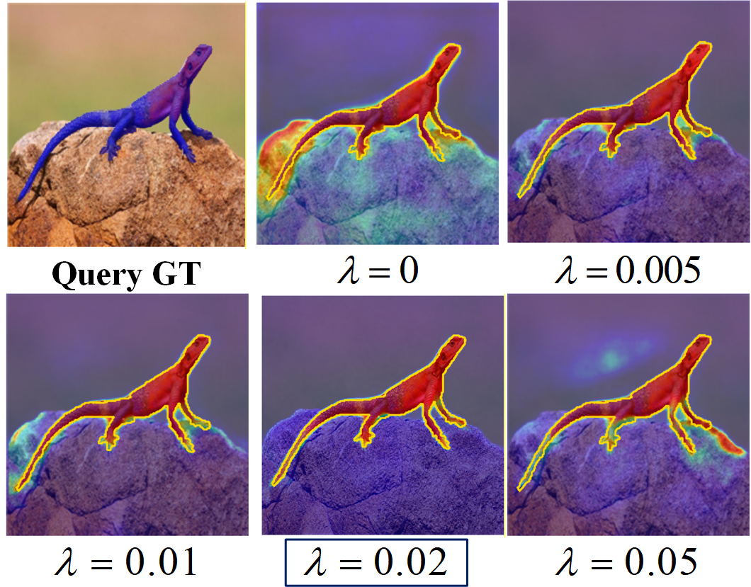
Table 3 shows that the uncertainty-aware constraint is most effective as a moderate regularizer. Increasing from 0 to 0.020 raises the four-domain mean from 70.7% to 72.6%, whereas a weight of 0.050 reduces it to 70.6%. Excessive contrastive weighting can overemphasize episode-level prototype relations at the expense of pixel-wise supervision. We therefore use as the default.
VACL Representation Visualization
Fig.4 (b) provides a feature-space view of VACL. Compared with HDH+PPR, the full model produces more compact foreground clusters and less foreground/background overlap in target domains, indicating that variance-derived prototype uncertainty is translated into a more separable decision space. The response maps under different weights further agree with Fig. 5: strengthens foreground-background discrimination without allowing the auxiliary objective to overwhelm segmentation supervision.
Conclusion
This paper reframes CD-FSS as a problem of maintaining reliable prototype discrimination under domain shift. DAUPNet implements this idea as a coherent chain: HDH stabilizes the hierarchical evidence used to construct prototypes, PPR exposes residual foreground-background uncertainty through probabilistic representation, and VACL uses variance-derived uncertainty to prevent unreliable comparisons from distorting the decision margin. Across four target domains, DAUPNet reaches 72.6%/76.7% average mIoU in the 1-shot/5-shot settings and improves the 1-shot baseline by 6.9% mIoU. Its strongest gains on weak-boundary and grayscale medical images demonstrate the practical value of uncertainty-aware prototype modeling, while the smaller gain on DeepGlobe indicates that global appearance alignment remains important when boundary ambiguity is not the dominant error source. These findings establish prototype reliability as a useful organizing principle for robust CD-FSS and motivate future work on jointly adapting uncertainty estimation and global domain alignment.
References
- Prototype as query for few shot semantic segmentation. Complex & Intelligent Systems 10 (5), pp. 7265–7278. Cited by: Cross-Domain Few-Shot Semantic Segmentation.
- Cross-domain few-shot semantic segmentation via doubly matching transformation. External Links: 2405.15265, Link Cited by: Cross-Domain Few-Shot Semantic Segmentation.
- Skin lesion analysis toward melanoma detection 2018: a challenge hosted by the international skin imaging collaboration (isic). arXiv preprint arXiv:1902.03368. Cited by: Datasets and Evaluation Metrics.
- Deepglobe 2018: a challenge to parse the earth through satellite images. In Proceedings of the IEEE conference on computer vision and pattern recognition workshops, pp. 172–181. Cited by: Datasets and Evaluation Metrics.
- The pascal visual object classes (voc) challenge. International journal of computer vision 88 (2), pp. 303–338. Cited by: Datasets and Evaluation Metrics.
- Self-support few-shot semantic segmentation. In Computer Vision – ECCV 2022, S. Avidan, G. Brostow, M. Cissé, G. M. Farinella, and T. Hassner (Eds.), Cham, pp. 701–719. External Links: ISBN 978-3-031-19800-7 Cited by: Few-Shot Semantic Segmentations.
- TraffiPrompt: network-aware multimodal prompt learning with motion-aware temporal modeling for driving video anomaly detection. International Journal of Intelligent Networks. Cited by: Cross-Domain Few-Shot Semantic Segmentation.
- Semantic contours from inverse detectors. In Proceedings of the 2011 International Conference on Computer Vision, ICCV ’11, USA, pp. 991–998. External Links: ISBN 9781457711015, Link, Document Cited by: Implementation Details.
- Deep residual learning for image recognition. 2016 IEEE Conference on Computer Vision and Pattern Recognition (CVPR), pp. 770–778. External Links: Link Cited by: Implementation Details.
- APSeg: auto-prompt network for cross-domain few-shot semantic segmentation. In 2024 IEEE/CVF Conference on Computer Vision and Pattern Recognition (CVPR), Vol. , pp. 23762–23772. External Links: Document Cited by: Table 1.
- Adapt before comparison: a new perspective on cross-domain few-shot segmentation. 2024 IEEE/CVF Conference on Computer Vision and Pattern Recognition (CVPR), pp. 23605–23615. External Links: Link Cited by: Cross-Domain Few-Shot Semantic Segmentation.
- Supervised contrastive learning. In Advances in Neural Information Processing Systems, H. Larochelle, M. Ranzato, R. Hadsell, M.F. Balcan, and H. Lin (Eds.), Vol. 33, pp. 18661–18673. External Links: Link Cited by: Variance-Aware Contrastive Learning Module.
- Few-shot segmentation via divide-and-conquer proxies. International Journal of Computer Vision 132 (1), pp. 261–283. Cited by: Cross-Domain Few-Shot Semantic Segmentation.
- Cross-domain few-shot semantic segmentation. In Computer Vision – ECCV 2022, S. Avidan, G. Brostow, M. Cissé, G. M. Farinella, and T. Hassner (Eds.), Cham, pp. 73–90. External Links: ISBN 978-3-031-20056-4 Cited by: Introduction, Cross-Domain Few-Shot Semantic Segmentation.
- Fss-1000: a 1000-class dataset for few-shot segmentation. In Proceedings of the IEEE/CVF conference on computer vision and pattern recognition, pp. 2869–2878. Cited by: Datasets and Evaluation Metrics.
- Robust few-shot segmentation for multi-modal medical images using fourier-guided style fusion and prototype alignment. Biomedical Signal Processing and Control 113, pp. 108986. Cited by: Cross-Domain Few-Shot Semantic Segmentation.
- The devil is in low-level features for cross-domain few-shot segmentation. In 2025 IEEE/CVF Conference on Computer Vision and Pattern Recognition (CVPR), Vol. , pp. 4618–4627. External Links: Document Cited by: Introduction, Cross-Domain Few-Shot Semantic Segmentation.
- Hypercorrelation squeeze for few-shot segmenation. 2021 IEEE/CVF International Conference on Computer Vision (ICCV), pp. 6921–6932. External Links: Link Cited by: Few-Shot Semantic Segmentations.
- Cross-domain few-shot segmentation via iterative support-query correspondence mining. In 2024 IEEE/CVF Conference on Computer Vision and Pattern Recognition (CVPR), Vol. , pp. 3380–3390. External Links: Document Cited by: Introduction, Cross-Domain Few-Shot Semantic Segmentation.
- Hierarchical dense correlation distillation for few-shot segmentation. 2023 IEEE/CVF Conference on Computer Vision and Pattern Recognition (CVPR), pp. 23641–23651. External Links: Link Cited by: Few-Shot Semantic Segmentations.
- Domain-rectifying adapter for cross-domain few-shot segmentation. In Proceedings of the IEEE/CVF Conference on Computer Vision and Pattern Recognition (CVPR), pp. 24036–24045. Cited by: Introduction, Cross-Domain Few-Shot Semantic Segmentation.
- Bridging granularity gaps: hierarchical semantic learning for cross-domain few-shot segmentation. In Proceedings of the AAAI Conference on Artificial Intelligence, Vol. 40, pp. 9215–9223. Cited by: Introduction, Cross-Domain Few-Shot Semantic Segmentation.
- Adapter naturally serves as decoupler for cross-domain few-shot semantic segmentation. In Forty-second International Conference on Machine Learning, External Links: Link Cited by: Table 1.
- Lightweight frequency masker for cross-domain few-shot semantic segmentation. In Advances in Neural Information Processing Systems, A. Globerson, L. Mackey, D. Belgrave, A. Fan, U. Paquet, J. Tomczak, and C. Zhang (Eds.), Vol. 37, pp. 96728–96749. External Links: Document, Link Cited by: Introduction, Cross-Domain Few-Shot Semantic Segmentation.
- Matching networks for one shot learning. In Proceedings of the 30th International Conference on Neural Information Processing Systems, NIPS’16, Red Hook, NY, USA. External Links: ISBN 9781510838819 Cited by: Implementation Details.
- PANet: few-shot image semantic segmentation with prototype alignment. In Proceedings of the IEEE/CVF International Conference on Computer Vision (ICCV), Cited by: Few-Shot Semantic Segmentations.
- Chestx-ray8: hospital-scale chest x-ray database and benchmarks on weakly-supervised classification and localization of common thorax diseases. In Proceedings of the IEEE conference on computer vision and pattern recognition, pp. 2097–2106. Cited by: Datasets and Evaluation Metrics.
- Personalize segment anything model with one shot. In The Twelfth International Conference on Learning Representations, External Links: Link Cited by: Table 1.
Appendix

HDH Mechanism Visualization
To further examine how Hierarchical Domain-Aware Harmonization (HDH) reorganizes multi-level features before prototype computation, we visualize the hierarchical responses and support-query cross-similarity of a representative FSS-1000 episode.
As shown in Fig.1(a), we compare the query-branch hierarchical responses before and after HDH, together with the support sample, query image, ground-truth mask, final prediction, and error map. Before HDH, responses across different levels are not fully aligned: shallow or mid-level features may retain local texture activations, while deep-level responses are semantically stronger but spatially coarser. After HDH, activations concentrate more on the target region and are less affected by scattered background textures, indicating that the hierarchical coordination path reorganizes multi-level features rather than simply amplifying response magnitudes.
As shown in Fig.1(b), we further visualize the support-query hierarchical cross-similarity matrix for the same episode. Each cell represents the cosine similarity between one supportlayer feature and one querylayer feature, with rows denoting support layers and columns denoting query layers. The Before HDHand After HDH matrices show the support-query correspondence before and after hierarchical coordination, while the After Before difference matrix reveals percell changes introduced by HDH. Positive values in the difference matrix indicate enhanced matching between corresponding support/query layers, while negative values indicate suppressed or weakened matching. The clearer diagonal structure and enhanced adjacent-layer alignment after HDH confirm that semantically related layers achieve more stable support-query alignment. These results are consistent with Table 2 in the main text, where HDH raises the mean mIoU from 65.7 to 69.7, and provide the feature-level basis for subsequent PPR prototype statistics.
PPR Prototype Modeling Ablation
To determine which prototype statistics best describe support samples, we conduct a controlled ablation of PPR prototype modeling strategies on FSS-1000, since this domain exhibits substantial variation in category morphology and foreground-background relationships, making it more sensitive to prototype quality.
| Exp. | Prototype Source | Variance | mIoU |
| 1 | Single deterministic | 78.5 | |
| 2 | Deepest-layer fg/bg | 78.1 | |
| 3 | Deepest-layer fg/bg | 80.0 | |
| 4 | Multi-level fg/bg | 77.7 | |
| 5 | Multi-level fg/bg | 77.7 |

| Exp. | Setting | Representation Path | VACL Input | Four-Domain Mean |
| 1 | Baseline | baseline feature | no VACL | 65.7 |
| 2 | Baseline + VACL | baseline feature | deterministic prototypes | 76.0 |
| 3 | HDH + VACL w/o PPR | HDH feature | HDH deterministic prototypes | 76.0 |
| 4 | HDH + PPR + VACL | HDH + PPR feature | PPR probabilistic prototypes and variances | 72.6 |
| Exp. | Setting | Variance Weight | Rank Weight | FG-BG Separation | FG Attraction | BG Attraction | mIoU |
| 1 | w/o VACL | 77.7 | |||||
| 2 | Standard contrastive | ✓ | ✓ | ✓ | 75.9 | ||
| 3 | Variance-aware contrastive | ✓ | ✓ | ✓ | ✓ | ✓ | 78.7 |
| 4 | Negative only | ✓ | ✓ | ✓ | 76.7 | ||
| 5 | Positive only | ✓ | ✓ | ✓ | ✓ | 75.1 | |
| 6 | FG positive + negative | ✓ | ✓ | ✓ | ✓ | 78.1 |

As shown in Table 1, we compare five configurations with distinct prototype sources and variance estimation strategies: simple deterministic prototype (Exp. 1), deepest-layer foreground/background prototypes without variance (Exp. 2), deepest-layer foreground/background prototypes with variance (Exp. 3), multi-level foreground/background prototypes without variance (Exp. 4), and full PPR with multi-level prototypes and variance estimation (Exp. 5). This comparison is organized around two factors: prototype source granularity (single vs. deepest-layer vs. multi-level) and whether variance estimation is incorporated. Since variance estimation depends on foreground/background prototype statistics, not all column combinations are semantically meaningful.
As shown in Table 1, the benefit of PPR primarily stems from changes in prototype statistics. Exp. 3 achieves the best result in this group (80.0), demonstrating that variance estimation provides necessary reliability modeling for prototypes. Exp. 4 and Exp. 5 further indicate that multi-level information requires coordination with hierarchical consistency and reliability modulation; otherwise, cross-level semantic discrepancies can dilute prototype quality. These results confirm that PPR is not simply introducing multi-level features, but rather constructing more reliable support-sample descriptions through foreground/background means and variances.
As shown in Fig.2, we decompose the PPR prototype modeling process into interpretable intermediate states on the same FSS-1000 episode. The figure sequentially presents: the support sample, query image with ground-truth mask, L4/L5 foreground responses, L4/L5 background responses, PPR-fused foreground response, PPR-fused background response, foreground/background uncertainty regions, and the error map from the HDH+PPR checkpoint. L4 responses better preserve edges, local textures, and fine-grained shape information, while L5 responses emphasize semantic targets but are spatially coarser. Consequently, single-level prototypes struggle to simultaneously capture target localization and boundary recovery. After PPR reorganizes multi-level foreground/background statistics into probabilistic prototypes, the fused foreground response indicates whether target regions are stably activated, and the fused background response reveals whether non-target regions and distracting textures are effectively suppressed. The foreground/background uncertainty map is constructed from the normalized difference between fused foreground and background responses: when the two responses are close, uncertainty is higher, typically concentrated around target boundaries, similar textures, and regions with strong foreground/background competition. The final PPR/Error map uses predictions from the HDH+PPR checkpoint (without VACL) to directly reveal residual false positives and false negatives after PPR prototype modeling. This visualization demonstrates that PPR does not merely enhance foreground heatmaps, but explicitly characterizes the competitive relationship between targets and backgrounds through paired foreground/background probabilistic prototypes, converting prototype uncertainty into observable boundary and confusion regions.
PPR-VACL Dependency Diagnostic
To verify whether the probabilistic prototypes and variance estimates provided by PPR effectively support VACL, we conduct a diagnostic experiment with two types of controls: first, adding VACL without full PPR to test whether the contrastive constraint has independent effects; second, comparing deterministic prototypes against PPR probabilistic prototypes to determine whether variance estimation provides more reliable weighting for VACL.
As shown in Table 2, the configurations are organized by the input source to VACL, focusing on how different prototype statistics support contrastive constraints.
As shown in Table 2, adding VACL under deterministic prototype conditions also improves performance, indicating that VACL does not require full PPR to take effect. Both Baseline+VACL and HDH+VACL w/o PPR outperform Baseline, confirming that foreground/background contrastive constraints inherently enhance feature discriminability. The full HDH+PPR+VACL configuration further introduces probabilistic prototypes and variance estimates from PPR, providing a reliability-aware basis for contrastive weighting. These results demonstrate that PPR not only provides probabilistic prototype representations, but also supplies reliability-stratified inputs to VACL, enabling contrastive learning to weight samples according to prototype reliability.
VACL Component Ablation
To further verify the necessity of VACL’s internal design, we conduct component ablation around variance weighting, rank weighting, and distinct contrastive terms.
As shown in Table 3, we compare six configurations organized from two perspectives: first, comparing standard contrastive learning against variance-aware contrastive learning to determine whether the gains stem from variance-aware weighting; second, decomposing VACL loss terms into foreground-background separation, foreground intra-class attraction, and background intra-class attraction to analyze the contributions of different contrastive relations. All experiments are conducted on FSS-1000.
As shown in Table 3, we compare six configurations organized from two perspectives: first, comparing standard contrastive learning against variance-aware contrastive learning to determine whether the gains stem from variance-aware weighting; second, decomposing VACL loss terms into foreground-background separation, foreground intra-class attraction, and background intra-class attraction to analyze the contributions of different contrastive relations. All experiments are conducted on FSS-1000.
As shown in Fig.3, the VACL analysis is organized across four dimensions: component ablation, weight response, reliability relations, and feature separation. Fig.3(a) compares w/o VACL, standard contrastive, negative only, positive only, FG positive + negative, and full VACL on the same episode using high-contrast error maps to observe how pixel-level errors migrate after introducing different loss terms. Green, red, and blue respectively indicate regions where predictions align with, overshoot, or undershoot the ground truth, enabling analysis of VACL’s impact on boundaries, background suppression, and foreground coverage. Fig.3(b) characterizes the weighting basis of VACL through inter-episode prototype similarity and reliability weights, including FG-FG similarity (cosine similarity between foreground prototypes across episodes), FG reliability weight (pairwise combinations of foreground prototype reliability weights), FG-BG similarity (cross-class similarity between foreground and background prototypes), and cross-class reliability weight (combined weighting strength of foreground and background reliability). Fig.3(c) quantifies changes in the foreground/background representation structure by comparing support prototype distance, query feature-center distance, and query pixel-prototype margin with VACL disabled versus enabled () across all four target domains.
Domain Distance and Target-Domain Performance
To further analyze the degree of domain shift across different target domains, we extract image features from the source domain (PASCAL VOC) and four target domains, and adopt RBF-kernel MMD with L2 normalization as the domain-distance metric. This analysis does not participate in model training; rather, it serves as a target-domain difficulty assessment: larger MMD distances indicate greater discrepancies between target and source feature distributions, under which models are typically more susceptible to background texture variations, imaging modality shifts, or object structure changes.
| Target Domain | MMD Distance | Baseline | DAUPNet | mIoU |
| DeepGlobe | 1.2 | 41.5 | 45.8 | 4.3 |
| ISIC | 0.6 | 68.6 | 73.0 | 4.4 |
| Chest X-ray | 0.8 | 78.3 | 91.3 | 13.0 |
| FSS-1000 | 0.9 | 74.4 | 80.1 | 5.7 |
Specifically, given source-domain feature set and target-domain feature set , we compute
| (1) |
where is the RBF kernel. In our implementation, features are first L2-normalized; the median of pairwise Euclidean distances between source and target feature subsets is used as the RBF bandwidth ; the final distance reported in Table 4-11 is the square root of the non-negative . We note that values depend on four factors: the feature extractor and selected feature layer, the sample size and category composition of source and target sets, feature normalization, and the RBF kernel bandwidth. Therefore, the values in Table 4 serve only for relative comparison of domain shifts across the four target domains under the same extractor, normalization, and kernel settings, and should not be directly compared with values computed under different configurations in other works.
As shown in Table 4, DeepGlobe exhibits the largest distance from the source domain, and its segmentation performance is substantially lower than other target domains, indicating that aerial imaging viewpoints, extensive background textures, and elongated road structures collectively create strong domain shift. ISIC has a relatively small distance, yet lesion boundaries and low-contrast regions still impose domain-specific medical challenges. FSS-1000 lies in the intermediate range, where DAUPNet achieves a notable gain over the baseline, suggesting that the full model compensates for morphological variations in natural long-tailed categories. Chest X-ray does not have the smallest distance, but its target structures are relatively stable and it benefits substantially from the complete modeling chain, yielding the highest mIoU among the four target domains.
Parameter Count, Computation, and Inference Efficiency
Beyond segmentation accuracy, we further quantify the parameter count, computational cost, inference speed, and memory usage of DAUPNet relative to the baseline. This analysis evaluates whether the HDH, PPR, and VACL structures introduce unacceptable computational overhead.
| Method | Input Size | Params | FLOPs | FPS | Memory |
| Baseline | 416 | 28.101M | 48.003G | 33.3 | 322.37 MB |
| DAUPNet | 416 | 28.578M | 50.313G | 21.7 | 360.76 MB |
| Baseline | 400 | 28.101M | 44.765G | 38.7 | 306.51 MB |
| DAUPNet | 400 | 28.578M | 46.903G | 28.8 | 341.89 MB |
As shown in Table 5, compared to the baseline, DAUPNet introduces only approximately 0.477M additional parameters, corresponding to a roughly 1.7% parameter increase. Under input sizes of 416 and 400, DAUPNet adds approximately 2.31G and 2.14G FLOPs, with memory usage increasing by approximately 38.39 MB and 35.38 MB, respectively. Inference speed decreases, indicating that hierarchical fusion and prototype inference introduce additional runtime overhead. Nevertheless, in terms of parameter count and memory usage, the complete model remains relatively lightweight.
Limitations Analysis
First, the 5-shot results on DeepGlobe fall below some recent methods, indicating that in remote sensing imagery, large-scale repetitive textures and complex backgrounds can still induce spuriously high-confidence predictions. This typically manifests as background confusion and boundary expansion, where the model misclassifies background regions with textures similar to the target as foreground.
Second, small objects, elongated structures, and partial occlusions in FSS-1000 increase the difficulty of prototype estimation. When the target region in the support sample is small, or when query-image targets exhibit substantial scale variation, the model may produce missed detections for small objects or under-segmentation of structural regions. This observation is consistent with Table 4-7, where multi-level prototypes did not show a stable advantage in the FSS single-domain diagnostic, suggesting that reliability conflicts persist between shallow details and high-level semantics.
Third, boundary ambiguity and low-contrast regions remain challenging in medical target domains such as ISIC and Chest X-ray. Although DAUPNet achieves high mIoU on medical domains, qualitative results indicate that the model may still produce boundary over-segmentation or local under-segmentation in regions with incomplete lesion edges or grayscale structural boundaries, suggesting room for improvement in boundary calibration.
These observations indicate that the primary failure modes of DAUPNet are concentrated in four categories: small-object missed detection, boundary over-segmentation, background confusion, and structural under-segmentation. Background confusion is associated with the complex remote sensing textures of DeepGlobe; small-object missed detection and structural under-segmentation relate to target scale and morphological variations in FSS-1000; and boundary over-segmentation more frequently occurs in weak-boundary medical images. These observations are consistent with the quantitative results and qualitative prediction figures presented in the main text.