

![[Uncaptioned image]](2607.13699v1/IFAE.png)
![[Uncaptioned image]](2607.13699v1/UAB.png)
![[Uncaptioned image]](2607.13699v1/Qilimanjaro.png)
MACHINE LEARNING DEVELOPMENT FOR QUANTUM COMPUTING AND NEUTRINO PHYSICS
A thesis presented for the degree ofDoctor of Physics by:
Annalisa De Lorenzis
| Supervisors: | M. Pilar Casado Lechuga |
| Thorsten Lux | |
| Arnau Riera Graells | |
| Tutor: | M. Pilar Casado Lechuga |
May 29, 2026
To my family, for their love and support.To the memory of my grandparents and uncles.To Luigi, for bringing light to the darkest days.To my past self, for not giving up.
Abstract
This thesis investigates the application of machine-learning methods in the context of quantum computing and neutrino physics, with particular emphasis on the construction of effective representations for complex, high-dimensional data.
The first part of the work is devoted to Quantum Extreme Learning Machines (QELMs), a hybrid quantum–classical framework in which classical data are encoded into quantum states and processed through fixed quantum dynamics, while learning is performed by a classical readout layer. Within this framework, we analyze the role of encoding strategies, feature-reduction methods, Hamiltonian structure, and measurement, with particular focus on the relationship between quantum dynamics, expressivity, entanglement, and classical simulability.
The second part of the thesis concerns the application of deep learning to the analysis of images produced by water Cherenkov detectors in neutrino physics. Convolutional architectures, including residual networks, are developed for the classification of complex events in realistic simulated datasets, showing that such models can effectively extract relevant information from detector data.
Taken together, these results highlight the potential of machine learning, in both its classical and quantum forms, as a powerful framework for the analysis of complex data in fundamental physics, while also outlining relevant challenges and directions for future research.
List of publications
The main results of this thesis are presented in these two papers:
-
1.
A. De Lorenzis, M. P. Casado, M. P. Estarellas, N. Lo Gullo, T. Lux, F. Plastina, A. Riera, J. Settino, “Harnessing Quantum Extreme Learning Machines for Image Classification,” Physical Review Applied 23, 044024 April, 2025. The article was later selected for inclusion in Quantum Frontiers, a curated collection by Physical Review Applied.
-
2.
A. De Lorenzis, M. P. Casado, N. Lo Gullo, T. Lux, F. Plastina, A. Riera, “Entanglement and Classical Simulability in Quantum Extreme Learning Machines,” Physical Review Applied, 25, 054052, May, 2026.
In addition, I am co-author of the following publications:
-
1.
Hyper-Kamiokande Collaboration, K. Abe et al., “Sensitivity of the Hyper-Kamiokande experiment to neutrino oscillation parameters using acceleration neutrinos”, Eur.Phys.J.C 86 (2026) 2, 170.
-
2.
Hyper-Kamiokande Collaboration, K. Abe et al., “The Hyper-Kamiokande experiment: input to the update of the European Strategy for Particle Physics”, arXiv: 2506.16641 [hep-ex], June, 2025.
-
3.
D. Attié et al., “Analysis of test beam data taken with a prototype of TPC with resistive Micromegas for the T2K Near Detector upgrade”, Nucl.Instrum.Meth.A 1052, 168248 July, 2023.
-
4.
L. Ambrosi et al., “Characterization of charge spreading and gain of encapsulated resistive Micromegas detectors for the upgrade of the T2K Near Detector Time Projection Chambers”, Nucl.Instrum.Meth.A 1056, 168534 November, 2023.
Chapter 1 Introduction
In the last few decades, many areas of science, technology, and society have undergone a profound and remarkably rapid digital transformation. Whereas in the past datasets were often relatively small and could be analyzed using simple, problem-specific tools, modern applications routinely generate massive, heterogeneous, and high-dimensional streams of data. Examples range from sensor networks, medical imaging, and financial markets to social media, recommendation systems, and large-scale scientific experiments. In this context, it has become essential to develop efficient techniques capable of handling large volumes of data and extracting from them reliable, interpretable, and actionable information.
A particularly powerful class of such techniques is provided by machine learning [bishop2006, Goodfellow-et-al-2016, geron2022], a broad family of methods designed to learn patterns and predictive rules directly from data. Rather than relying exclusively on handcrafted features or explicit physical models, machine-learning algorithms adapt their internal parameters to examples, thereby discovering structures that may be difficult or impossible to encode by hand. These methods now play a central role in a wide range of applications, including image and speech recognition, natural language processing, anomaly detection, and data-driven scientific discovery.
In parallel to these developments, the increasing complexity of physical systems and data representations raises fundamental computational challenges. The intrinsic difficulty of simulating quantum systems on classical computers was first emphasized by Richard Feynman [feynman1982simulating, Nielsen_Chuang_2010, Montanaro_2016, Preskill:2018jim], who suggested that quantum devices may provide a natural framework for modeling physical processes that are otherwise computationally intractable [Arute48651, Huang:2021pei].
Within this broader context, quantum machine learning (QML) [Biamonte:2016ugo, Schuld:2018gao, Schuld:2018uel, book, Congarticle, Liu:2022bpb, Lloyd:2013lby, Schuld2014, Havlicek:2018nqz] has emerged as an active research area at the interface between quantum computing and machine learning, with the goal of exploiting quantum systems and algorithms for data analysis, representation learning, and classification tasks. Among the different QML approaches, Quantum Extreme Learning Machines (QELMs) [DeLorenzis_1, DeLorenzis_2, Sakurai:2022ala, Hayashi:2022xab, Hayashi:2025gwk, Sakurai_simpleH, QELMSuprano, Vetrano:2024vbh, Innocenti2023] provide a particularly attractive hybrid framework, since they combine quantum feature generation with a simple classical readout layer.
The present thesis is situated within this broader landscape and lies at the intersection of machine learning, quantum computing, and neutrino physics. On the one hand, it investigates QELMs for supervised classification tasks, with particular emphasis on the role of data encoding, feature reduction, quantum dynamics, and measurement in the construction of effective representations of classical data. On the other hand, it develops and applies deep-learning techniques to the analysis of neutrino detector images. Despite the apparent difference between these two research directions, they are united by a common objective: the construction of effective representations of complex, high-dimensional data. In both settings, the central challenge is to design models that transform raw inputs into feature spaces in which relevant patterns can be extracted in an efficient, robust, and physically meaningful way.
More specifically, the work presented in this thesis is organized around two complementary research directions.
The first research direction concerns QELMs, a class of hybrid quantum–classical models inspired by reservoir computing [Sakurai:2022ala, AngelatosPhysRevX.11.041062, Mujal_2021, Domingo:2022fre, Martinez2021, Fujii2017, chenPhysRevApplied.14.024065] and by the extreme learning machine (ELM) paradigm [HUANG2006489, articleHuang2011, wang2022review, markowska-kaczmar_extreme_2021, 10.1007/s10462-013-9405-z, Huang_extreme2]. In the framework studied here, the processing pipeline is decomposed into four stages: a classical preprocessing step that compresses the input data, a quantum encoding map that prepares an -qubit state, a fixed unitary evolution generated by a many-body Hamiltonian, and a measurement stage whose outcomes define a classical feature vector processed by a shallow readout network. Unlike variational quantum models [Peruzzo:2013bzg, Farhi:2014ych, Cerezo:2020jpv], the quantum part of the architecture is not optimized through an iterative training loop: the encoding, the Hamiltonian, the evolution time, and the measurement prescription are fixed in advance, while all trainable parameters are confined to the final classical classifier. This makes QELMs a useful setting in which to study the representational role of quantum dynamics itself, disentangled from the optimization difficulties of deep parameterized circuits.
A central technical issue in this framework is the embedding of high-dimensional classical data into a small quantum register without discarding the information most relevant for classification. For this reason, a substantial part of the thesis is devoted to the interplay between classical compression and quantum encoding. We consider both linear and nonlinear feature-reduction strategies, in particular Principal Component Analysis and convolutional autoencoders, and we compare several encoding schemes, including simple angle, dense-angle, uniform Bloch-sphere, general, and amplitude encodings. We also analyse different interacting Hamiltonians for the quantum layer and investigate how the corresponding measurement statistics can be exploited by a shallow classical readout.
These ingredients are first studied in a systematic image-classification analysis on standard benchmarks such as MNIST [mnist] and Fashion-MNIST [fashionmnistnovelimagedataset], and later revisited in a more controlled setting including CIFAR-10 [cifar10]. The first study shows that the preprocessing stage is already decisive in the strongly compressed regime relevant to near-term quantum models: nonlinear latent representations produced by autoencoders consistently outperform PCA, and this advantage persists on the more challenging Fashion-MNIST dataset. The comparison between encoding strategies further shows that dense-angle and uniform Bloch-sphere encodings provide the most favourable balance between accuracy and implementability, since they exploit two Bloch-sphere parameters per qubit while remaining compatible with relatively shallow state-preparation circuits. Amplitude encoding is more compact in terms of qubit resources, but becomes competitive only when sufficiently many latent features are injected into the amplitudes, which in turn makes state preparation more demanding.
The same study also clarifies the role of the quantum evolution. Once the latent representation and the encoding are fixed, the classification accuracy increases rapidly with the number of qubits and reaches a plateau around . In this regime, the performance becomes largely insensitive to the microscopic details of the interacting Hamiltonian, indicating that the relevant ingredient is not a finely tuned model of dynamics, but rather the ability of the evolution to redistribute the encoded information into a measurement space more suitable for the final classifier. With this architecture, QELMs reach accuracies comparable to, and in some cases better than, several previously proposed hybrid quantum–classical models for image classification [DeLorenzis_1].
The second QELM study focuses on the relation between classification performance, entanglement growth, and classical simulability. In this part of the thesis, the architecture is fixed more rigidly: the latent classical features are encoded through dense-angle encoding, the quantum layer is implemented by a nearest-neighbour XX Hamiltonian with periodic boundary conditions, and the only continuous hyperparameter varied is the evolution time . This setup allows one to analyse, in a controlled way, how the dynamics of the quantum layer correlates with the quality of the generated features across MNIST, Fashion-MNIST, and CIFAR-10.
A central result is that the QELM accuracy displays a sharp transition as a function of : after an initial low-performance region, both training and test accuracies rise rapidly around a characteristic time and then saturate to a plateau. Remarkably, the location of this transition is essentially independent of system size, suggesting that the relevant timescale is set by local dynamical processes rather than by the total number of qubits. Moreover, the plateau accuracy coincides, within numerical uncertainties, with that obtained by replacing the XX evolution with Haar-random unitaries acting on the same encoded states.
This observation motivates a more refined interpretation of the role of quantum dynamics in QELMs. The onset of useful feature generation does not require fully scrambled states or highly nonlocal entanglement. Instead, the relevant regime is associated with the build-up of local entanglement and with the spreading of information over a finite range, consistent with a local dynamical timescale. The thesis further shows that this regime remains compatible with efficient tensor-network simulation and can be reproduced, to a large extent, by shallow random circuits with local gates. The results therefore do not provide evidence for a generic quantum advantage, but they do identify a physically meaningful intermediate regime in which quantum dynamics enriches the representation of classical data while remaining structurally close to models that are still classically tractable [DeLorenzis_2].
The second research direction of the thesis concerns the application of machine learning to neutrino physics, with particular emphasis on the classification of complex event topologies in water Cherenkov detectors. The experimental context is the Hyper-Kamiokande [Hyper-Kamiokande:2018ofw, Hyper_2015, Hyper-Kamiokande:2025fci, Hyper-Kamiokande:2025asb] programme and, more specifically, its Intermediate Water Cherenkov Detector (IWCD), a cylindrical detector instrumented with multi-PMT optical modules. In this setting, neutrino interactions are not observed directly; rather, they are inferred from the charge and timing patterns produced by Cherenkov light on the detector surface. A crucial technical step is therefore the construction of a suitable image representation of the detector response. In this thesis, the cylindrical surface is unwrapped into a rectangular grid in coordinates, and the charge and timing information associated with the photosensors is organised into image channels, yielding multi-channel detector images that can be processed by convolutional architectures.
The supervised task considered in detail is the discrimination between single-vertex and pile-up events. Single-vertex events contain one neutrino interaction in the relevant time window, but may still exhibit non-trivial multi-ring topologies because of the multiplicity of charged particles in the final state. Pile-up events instead contain two or more independent interactions within the same detector readout window, producing overlapping Cherenkov patterns that are more difficult to disentangle. This is therefore a physically relevant classification problem for high-rate near detectors, where one seeks robust discrimination based not only on total light yield but also on the spatial and temporal structure of the event.
To address this problem, the thesis develops a ResNet-18–based convolutional classifier [he2016deep] tailored to IWCD images. The adopted network preserves the residual structure of the standard ResNet-18 architecture, with four residual stages, but modifies the input stem to better preserve fine spatial information in detector images.
The results show that deep convolutional models are highly effective for this task. When both charge and timing information are used in the non-compact representation, the classifier reaches Area Under the Curve (AUC) values close to unity on both simplified topological samples and more realistic generator-level event samples. Timing information emerges as especially informative for separating single-vertex from pile-up events, while compact representations remain competitive with the full non-compact input.
Additional studies as a function of event-level variables show that the classification becomes more difficult when the interaction vertices are close in space and time, or when the event develops near detector boundaries, in agreement with the physical picture of strongly overlapping or partially truncated Cherenkov patterns.
Finally, the thesis includes an exploratory transfer of the QELM framework to realistic neutrino-image data. Because present QELM implementations require strong compression of the classical input, this study is intentionally preliminary. Detector images are reduced to low-dimensional feature vectors, encoded into 10-qubit states through Bloch-sphere encoding, evolved with an XX-type Hamiltonian, and classified through a single sigmoid readout. Even in this constrained setting, the QELM extracts non-trivial discriminating information from IWCD events, with the mixed charge-plus-timing representation giving the best performance among the tested configurations. Although the results remain significantly below those obtained with ResNet-18, they show that the QELM pipeline can be meaningfully transferred from standard image benchmarks to realistic detector data. In addition to the analyses presented in this part of the thesis, I also contributed, together with other collaborators, to the development of the open-source WatChMaL framework [WatChMaL], in particular to the introduction of timing information in the analysis pipeline.
Main contributions of the thesis.
The main contributions of this thesis can be summarized as follows. First, it develops and formalizes a QELM pipeline for supervised image classification in which the effects of feature reduction, encoding, Hamiltonian choice, and measurement can be analysed separately. Second, it shows that, in the compressed regime relevant to near-term quantum models, nonlinear latent representations obtained through autoencoders are more effective than PCA, and that dense-angle-type encodings provide a particularly favourable trade-off between performance and implementability. Third, it demonstrates that high QELM performance can be reached without highly specific Hamiltonian engineering, and that in the XX-based setting the relevant operating regime is associated with local entanglement growth and remains compatible with efficient classical simulation. Fourth, it develops a ResNet-18–based framework for the classification of IWCD single-vertex and pile-up events from multi-channel charge-and-timing images, achieving robust performance across multiple simulated datasets. Fifth, it presents a first proof-of-concept application of the QELM framework to realistic neutrino-image data, thereby establishing a concrete connection between the two main parts of the thesis.
Structure of the thesis.
The remainder of this thesis is organized as follows. Chapter 2 introduces the machine-learning concepts used throughout the thesis, including supervised learning, neural networks, optimization, evaluation metrics, autoencoders, and convolutional architectures. Chapter 3 reviews the aspects of quantum computing most relevant for the present work, with emphasis on Hilbert-space representations, unitary dynamics, and measurement as ingredients of quantum feature generation. Chapter 4 presents the general QELM framework and describes in detail the classical preprocessing stage, the encoding strategies, the Hamiltonians used for the quantum layer, the measurement stage, and the classical readout. Chapter 5 applies this framework to image classification and analyses the impact of feature reduction, encoding, and Hamiltonian choice. Chapter 6 studies in greater depth the relationship between performance, entanglement growth, information spreading, and classical simulability in XX-based QELMs. Chapter 7 introduces the physical context of neutrino detection, Cherenkov radiation, and water Cherenkov detectors, with particular attention to Hyper-Kamiokande and the IWCD. Chapter 8 develops and evaluates deep-learning models for neutrino detector images and includes an exploratory QELM application to the same classification problem. Finally, Chapter 9 summarizes the main results and discusses possible future directions.
Chapter 2 Machine Learning Background
2.1 Historical overview
The term machine learning was introduced in the late 1950s by Arthur Samuel [Samuel], a pioneer in computer gaming and artificial intelligence, who developed one of the first programs capable of improving its own performance at the game of checkers through experience. The conceptual origins of the field, however, are broader and lie in the study of human cognitive processes. In 1949, Donald Hebb [hebb1949] proposed a theoretical model of an artificial neuron and a learning mechanism based on the strengthening of synaptic connections, which would profoundly influence the development of neural networks. A few years earlier, Walter Pitts and Warren McCulloch [mcculloch1943] introduced an early mathematical formalization of networks of logical neurons, showing how simple binary units can, in principle, implement complex computations.
In the following decades, the first devices and algorithms able to learn from data were developed. In the 1960s, so-called learning machines appeared, designed to recognise patterns in signals such as sonar traces, electrocardiograms, or speech waveforms, often using elementary reinforcement mechanisms. Interest in pattern recognition and automatic classification continued throughout the 1970s and 1980s, with the development of statistical models and techniques such as principal component analysis for dimensionality reduction.
An important turning point occurred between the 1980s and 1990s, with the rediscovery and widespread adoption of the backpropagation algorithm [rumelhart1986] for training multi-layer neural networks and the introduction of kernel-based methods such as support vector machines [cortes1995]. During this period, an operational definition of machine learning [bishop2006, geron2022], often attributed to Tom Mitchell, became established: a program is said to “learn” if its performance on a given task improves with experience, with respect to a quantitative performance measure. At the same time, the distinction between supervised, unsupervised, and reinforcement learning took shape and remains at the core of modern taxonomies.
Starting from the late 2000s, so-called deep learning [lecun2015, he2016deep] brought about a further transformation. The combination of more powerful hardware (in particular graphics processing units GPUs), large annotated datasets, and new neural architectures made it possible to train very deep networks with millions of parameters, capable of achieving state-of-the-art performance in tasks such as image classification, speech recognition, and natural language processing. Among the most emblematic results of this period are the introduction of generative adversarial networks (GANs) [Goodfellow-et-al-2016], able to synthesise realistic data, and the successes of deep reinforcement-learning systems such as AlphaGo [Silver2016MasteringTG], which have surpassed the best human players in highly complex board games.
In this thesis we do not attempt to provide an exhaustive historical survey, but rather focus on the fundamental concepts that are most relevant for the applications to quantum computing and neutrino physics discussed in the following chapters.
2.2 Supervised and unsupervised learning
At a high level, a machine-learning problem can be described in terms of data, models, and a learning objective. We are given a dataset with input with (e.g. an image, a time series, or a feature vector) and, depending on the task, a target (e.g. a class label or a real-valued output). We then choose a family of models , such as a neural network, parametrized by and an objective function that quantifies how well matches the data. Learning consists in adjusting so as to minimize on the training data, while still performing well on unseen examples.
In supervised learning, each input is associated with an explicit target . The goal is to learn a mapping that predicts the correct output for new, unseen inputs. Typical supervised tasks include:
-
•
classification, where is a discrete class label (e.g. neutrino vs. background event);
-
•
regression, where is a real-valued quantity (e.g. an energy or a continuous parameter).
In unsupervised learning, only the inputs are given, and there are no explicit targets. The objective is to identify structure in the data, such as clusters or low-dimensional manifolds. Examples include clustering algorithms (-means, Gaussian mixture models) and dimensionality reduction methods (Principal Component Analysis, autoencoders). In this thesis, unsupervised methods are mainly used for feature extraction and dimensionality reduction, for instance to compress high-dimensional images into a latent representation.
2.3 Neural Networks
Over the past decade, neural networks have become one of the central tools in modern machine learning. They are at the core of many applications in computer vision, natural language processing, game playing and scientific data analysis. Their success stems from their ability to approximate complex nonlinear functions directly from data, with minimal feature engineering.
At a high level, a neural network [Goodfellow-et-al-2016] is a function with parameters (usually called weights and biases) adjusted (trained) so that produces a desired output when given an input . The training process is guided by data and an objective (loss) function that quantifies how well the network performs on a particular task. By minimizing this loss over a training dataset, the network learns patterns present in the data and can then be used to make predictions on unseen examples.
Although the name “neural network” originates from analogies with biological neurons, modern neural networks are best viewed as compositions of simple mathematical operations. In what follows, we first introduce the basic computational unit, the neuron, and the way neurons are combined to form a network. We then describe the loss function, the optimization procedure used for training, and the metrics used to evaluate performance.
2.3.1 The neuron
The fundamental building block of a neural network is the neuron. Conceptually, a neuron receives one or more real-valued inputs, linearly combines them, and passes the result through a nonlinear activation function to produce an output.
Let denote the input vector to a neuron. The neuron is associated with a weight vector and a bias term . Its output is given by
| (2.1) |
where is a nonlinear activation function. Common choices include:
-
•
The rectified linear unit (ReLU), . It is piecewise linear, computationally cheap, and does not saturate in the positive region, which helps maintain stronger gradients in deep models. For these reasons, ReLU (and its variants, such as Leaky ReLU and ELU) has become the default choice for hidden layers in many deep-learning architectures.
-
•
The hyperbolic tangent, . Historically, was widely used in hidden layers, but it has been largely superseded by ReLU, since the hyperbolic tangent saturates for large .
-
•
The logistic (sigmoid) function, . It has historically been used in the output layer for binary classification, as it can be interpreted as a probability. However, in hidden layers it tends to suffer from saturation (very small gradients for large ), which can slow down training in deep networks.
The activation functions described above, together with some other examples such as the perceptron, are shown in Fig. 2.1.
The perceptron (or binary step) activation function,
played an important historical role in early neural-network models. However, it is rarely used in modern deep networks because it is non-differentiable and has zero gradient almost everywhere, making gradient-based optimization ineffective.

The nonlinearity of is crucial. Without it, a network of neurons would collapse to a single linear transformation, unable to model complex relationships. The combination of linear operations and nonlinear activations allows neural networks to approximate highly nonlinear functions.
2.3.2 Layers and feed-forward networks
In practice, neurons are organized into layers. A layer takes as input a vector of activations from the previous layer and outputs a new vector of activations. The simplest and most common architecture is the feed-forward (or fully connected, or dense) network. An example of a feed-forward architecture is shown in Fig. 2.2.

Consider a network with layers (excluding the input). Let be the input, and for ,
| (2.2) |
where:
-
•
is the weight matrix of layer ,
-
•
is the bias vector,
-
•
is applied element-wise to the pre-activation vector .
The vector is the output of the network. Depending on the problem, the output layer may use a specific activation:
-
•
For regression, a linear output () is often used.
-
•
For binary classification, a sigmoid activation is common.
-
•
For multi-class classification, the softmax function is typically used:
(2.3)
Networks with many hidden layers (layers between input and output) are called deep neural networks. A central theoretical result, the universal approximation theorem [cybenko1989, hornik1989], states that, under mild conditions, such networks can approximate any continuous function on a compact domain, provided they have enough units. In practice, depth and width must be chosen carefully to balance expressivity, computational cost and the risk of overfitting.
While fully connected networks are the conceptual baseline, many specialized architectures exist, such as, for example, Convolutional Neural Networks (CNNs) which exploit spatial structure and are well suited for image data; Recurrent Neural Networks (RNNs), designed to process sequential data; autoencoders that learn low-dimensional representations by reconstructing their input, etc. We will provide more details on some of these architectures later in this thesis.
2.4 Loss Functions
To train a neural network, one must quantify how well the network performs on a given task. This is the role of the loss function (also called the cost or objective function) [bishop2006]. Given an input–output pair and network prediction , the loss function measures the discrepancy between and . Training aims to find parameters that minimize the average loss over a training dataset.
The loss function on the entire training set is given by
| (2.4) |
and the explicit choice of depends on the particular task.
-
•
For regression problems, where (or ), a common choice is the mean squared error (MSE), defined as
(2.5) MSE penalizes large errors more strongly than small ones and is differentiable everywhere.
-
•
For classification, losses are typically based on likelihood. In the Binary classification case, for , with output interpreted as the probability of class 1, a common choice is the binary cross-entropy loss:
(2.6) -
•
In the multi-class classification case, instead, with classes and one-hot target vector (with for the true class , zero otherwise), one often uses the categorical cross-entropy:
(2.7) where is the softmax output of the network. This loss is equivalent to the negative log-likelihood of the correct class under the predicted distribution of the model.
2.5 Optimization
Training a neural network corresponds to minimizing the loss with respect to the parameters . Because is typically non-convex and high-dimensional, we rely on iterative, gradient-based optimization methods.
2.5.1 Gradient descent and backpropagation
The basic idea of gradient descent is to update the parameters in the direction of steepest descent of the loss:
| (2.8) |
where is the learning rate. The correct choice of this hyperparameter can be crucial for an efficient optimization. Indeed, a small learning rate may lead to slow convergence, while a learning rate that is too large can cause divergence or oscillations.
For neural networks, computing the gradient efficiently is made possible by the backpropagation algorithm, which applies the chain rule of calculus layer by layer, starting from the output.
However, computing the gradient using all training examples at each step (batch gradient descent) can be computationally expensive. Instead, we could use
-
•
Stochastic Gradient Descent (SGD), in which case gradients are estimated on a single example at a time;
-
•
Mini-batch gradient descent in which case gradients are computed on small batches of size , balancing stability and speed:
(2.9) where is a mini-batch and
(2.10)
One full pass over the entire training set is called an epoch. Training thus proceeds over multiple epochs, during which the network parameters are gradually updated.
2.5.2 Advanced optimization algorithms
Several extensions of basic gradient descent methods have been proposed to improve convergence, such as:
-
•
Momentum, accelerating learning by accumulating a velocity vector in parameter space, smoothing out noisy gradient fluctuations.
-
•
Adam (Adaptive Moment estimation), adapting the learning rate for each parameter based on estimates of first and second moments of the gradients. It is widely used due to its robustness and ease of use.
-
•
RMSProp, adapting learning rates based on gradient history.
The choice of optimizer and learning rate schedule can significantly affect training speed and final performance. Often, a learning rate that decays over time (step decay or exponential decay) improves convergence. In this thesis we mainly employ the Adam optimizer, as implemented in standard deep-learning libraries, both for classical networks and for the classical readout of the QELM.
2.5.3 Training, validation and test sets
A central concept in machine learning is that of generalization: a good model should not only fit the training data, but also perform well on new inputs drawn from the same underlying distribution. To evaluate generalization, the available data are usually split into non-overlapping subsets:
-
•
a training set, used to optimize the model parameters;
-
•
a validation set, used for model selection and hyperparameter tuning;
-
•
a test set, used only at the end of the analysis to estimate the final performance.
The optimization uses only the training set; the validation set guides decisions such as model architecture, regularization strength and early stopping.
Two important failure modes in the training of supervised learning models are overfitting and underfitting. A model underfits when it is too simple or trained for too few epochs, failing to capture the relevant structure in the data (high training and validation error). A model overfits when it fits the training data extremely well but fails to generalize to new examples (low training error but high validation error). Regularization techniques such as weight decay, dropout and early stopping, together with appropriate model capacity and careful monitoring of validation metrics, are essential to strike a balance between these two extremes.
In the remainder of the thesis, we will highlight overfitting/underfitting effects whenever relevant, in particular when comparing different architectures or training regimes.
2.6 Evaluation Metrics
While the loss function guides optimization, it does not always correspond directly to the quantity we ultimately care about. For example, in classification we may minimize cross-entropy but evaluate performance using accuracy, precision or other task-specific metrics. It is therefore important to define appropriate metrics [bishop2006] to assess model quality on validation and test data. For regression tasks, a commonly used metric is the Mean Squared Error (MSE), defined as in Eq. 2.5. For classification tasks, the simplest metric is accuracy, defined as
| (2.11) |
In particular, for binary classification problems, it is useful to introduce the confusion matrix, which counts the number of:
-
•
true positives (TP): positive samples correctly classified;
-
•
true negatives (TN): negative samples correctly classified;
-
•
false positives (FP): negative samples misclassified as positive;
-
•
false negatives (FN): positive samples misclassified as negative.
The overall accuracy is then defined as
| (2.12) |
However, when classes are imbalanced, accuracy may be misleading. In such cases, additional metrics are informative:
-
•
Precision (for a given class, say “positive”):
(2.13) answering the question “of all predicted positives, how many were correct?”
-
•
Recall (or sensitivity):
(2.14) answering the question “of all actual positives, how many did we find?”
-
•
F1 score, the harmonic mean of precision and recall:
(2.15)
Other tools include confusion matrices, Receiver Operating Characteristic (ROC) curves, and the Area Under the ROC Curve (AUC), which assess performance across different decision thresholds. Many classifiers output a continuous score or probability for the positive class. By varying a decision threshold and assigning samples with to the positive class, one obtains different trade-offs between:
-
•
the true positive rate (TPR or sensitivity),
-
•
the false positive rate (FPR),
The ROC curve plots TPR versus FPR as the threshold is varied. The AUC is a threshold-independent summary of classifier performance: an AUC of 0.5 corresponds to random guessing, whereas an AUC of 1.0 indicates perfect classification.
For multi-class classification, the confusion matrix is a table, where is the number of classes. The entry in row and column records how many samples of true class were predicted as class . Visualizing the confusion matrix provides insight into which classes are systematically confused with each other.
Throughout this thesis we will report accuracy and AUC values, as well as confusion matrices, to assess and compare the performance of the classical and quantum-inspired models introduced in the following chapters.
2.7 Convolutional Neural Networks
The fully connected networks introduced in the previous sections treat their inputs as generic vectors in , ignoring any particular structure the data might possess. However, many types of data, in particular images (such those in the MNIST [mnist] and CIFAR-10 [cifar10] datasets or the detector images in neutrino physics), exhibit strong local correlations and are naturally organized on regular grids. Convolutional Neural Networks (CNNs) [lecun98] are specifically designed to exploit such structure, and they form the backbone of most modern architectures in computer vision and related domains.
The key idea behind CNNs is to replace generic linear transformations with convolutional layers, in which small learnable filters (or kernels) are applied locally and repeatedly across the input. This induces parameter sharing (the same filter is used at all spatial locations) and sparse connectivity (each output unit depends only on a small neighborhood), which significantly reduces the number of parameters and improves statistical efficiency.
2.7.1 Convolutions and feature maps
For concreteness, consider a 2D input (e.g. a grayscale image) represented by a matrix , where and are the height and width. A convolutional layer applies a set of learnable filters , each of size , to the input. The output of filter is a feature map , whose entries are given by the discrete convolution
| (2.16) |
where is a nonlinear activation function (e.g. ReLU) and is a bias term associated with filter . In practice, convolutions may be implemented with a stride greater than 1 (skipping some positions) and with padding (zero-padding the input at the boundaries) to control the spatial dimensions of the output.
For multi-channel inputs (e.g. RGB images or feature maps from previous layers), each filter has the form , where is the number of input channels. A schematic illustration of this operation is shown in Fig. 2.3. The convolution then sums the contributions over channels:
| (2.17) |
Stacking all feature maps along a new channel dimension yields the output tensor of the convolutional layer, with shape (where and depend on stride and padding).
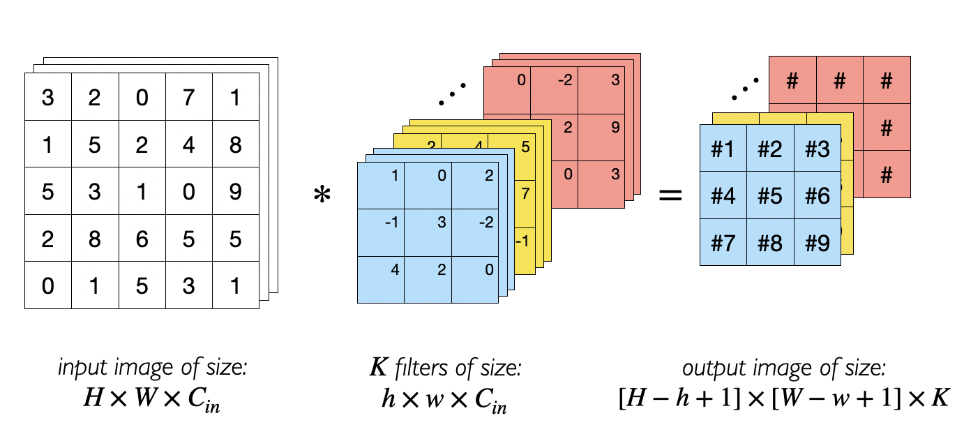
Intuitively, each filter learns to respond to a particular local pattern (e.g. an edge or a texture) and deeper layers combine these local patterns into more complex and abstract features.
2.7.2 Pooling and upsampling
Convolutional layers are often interleaved with pooling (or subsampling) layers, whose role is to reduce the spatial resolution while preserving the most salient information. A common choice is max pooling, which partitions each feature map into non-overlapping (or partially overlapping) regions and outputs the maximum value in each region, as illustrated in Fig. 2.4. In particular, a max-pooling operation reduces the height and width of the feature map by a factor of 2:
| (2.18) |
Other pooling operations include average pooling (taking the mean instead of the maximum) or more general aggregation functions.
Pooling has two main effects:
-
•
it reduces the dimensionality of the feature maps, lowering computational cost and the risk of overfitting;
-
•
it provides a degree of translational invariance, as small shifts of the input have limited effect on the pooled outputs.
In modern architectures, pooling is sometimes replaced or complemented by strided convolutions, which jointly perform feature extraction and downsampling.
In decoder-like parts of convolutional architectures, such as the decoder of a convolutional autoencoder, one often needs to increase the spatial resolution of the feature maps, effectively inverting the action of pooling or strided convolutions. This is achieved through upsampling layers. A common choice consists in a simple interpolation-based upsampling (e.g. nearest neighbour or bilinear interpolation). In a typical encoder-decoder architecture, downsampling layers in the encoder compress the input into a compact latent representation, while corresponding upsampling layers in the decoder progressively restore the original resolution, allowing the network to produce detailed reconstructions in the output space.

2.7.3 Typical CNN architectures
A typical CNN for image processing consists of a sequence of convolutional layers (possibly grouped into blocks), each followed by nonlinear activations and optionally pooling or normalization layers, progressively transforming the input into higher-level feature maps. In many architectures, the spatial resolution is gradually reduced while the number of channels increases, trading spatial detail for high-level feature extraction.
Eventually, the high-level features are fed into one or more fully connected layers (sometimes after global pooling operations) to produce the final output, such as class scores for classification or real-valued predictions for regression, see for instance Fig. 2.5. The entire network is trained end-to-end using the same gradient-based optimization techniques described in the previous section, with a suitable loss function depending on the task.Among the many convolutional architectures developed in deep learning, residual networks (ResNets) are of particular importance, as they enable the effective training of deeper models. We briefly review their main ideas in the next subsection.

2.7.4 Residual neural networks
Residual Networks
Empirically, very deep CNNs, with many convolutional layers, tend to be more expressive and capable of learning increasingly complex features. However, in practice, simply stacking more layers often leads to optimization difficulties and degraded performance.
Residual Networks (ResNets) [he2016deep] were proposed to address this problem by introducing shortcut connections that allow information and gradients to flow more easily through very deep architectures. ResNets make it possible to train networks with even hundreds of layers using standard optimization techniques, and they have become a standard building block in modern deep learning.
In practice, training very deep plain CNNs (without shortcut connections) often leads to a phenomenon known as the degradation problem.
As the depth increases beyond some point, the training error of a plain network starts to increase, even though the network has strictly more parameters. This degradation is not primarily due to overfitting since it appears on the training error, but rather to optimization difficulties: gradients can become very small (vanishing gradient problem) or very large (exploding gradient problem) as they propagate through many nonlinear layers, making it hard for standard gradient-based methods to find good solutions.
Residual networks address this issue by explicitly parameterizing the layers to learn deviations from the identity mapping, rather than the full mapping itself and this simple idea greatly facilitates the training of very deep models.
Residual blocks Consider a stack of layers that takes an input feature vector and produces an output . In a traditional CNN, the network directly learns the mapping
| (2.19) |
Residual learning instead reparameterizes the problem in terms of a residual function :
| (2.20) |
where is typically a small stack of convolutional layers with parameters collectively denoted by . The term is added to the output through an explicit shortcut connection. Equation (2.20) can be interpreted as learning the difference between the desired mapping and the identity:
| (2.21) |
If the identity mapping is optimal for some layers, then it should be easier to drive the residual towards zero than to force a stack of nonlinear layers to approximate the identity itself.

Figure 2.6 typically depicts a residual block as two or three convolutional layers whose output is summed with the original input through a shortcut path. A nonlinearity (such as ReLU) is often applied after the addition.
Identity and projection shortcutsIn the simplest case, the input and output of the residual block have the same dimension, and the shortcut connection is a pure identity:
| (2.22) |
This is referred to as an identity shortcut. Identity shortcuts have no additional parameters and negligible computational cost.
In deeper stages of the network, it is often necessary to change the spatial resolution or the number of channels (for example, to downsample the feature maps and increase the number of filters). In those cases, the shortcut performs a projection so that the dimensions match:
| (2.23) |
where is typically a convolution with stride greater than one (for spatial downsampling) and an appropriate number of output channels. This is known as a projection shortcut.
Both identity and projection shortcuts ensure that the gradient can flow directly from deeper layers to shallower ones, reducing vanishing/exploding-gradient effects and making optimization more stable.
ResNet Architectures
Residual blocks can be used as building blocks to construct deep architectures of varying depth. The basic residual block consists of two convolutional layers with the same number of output channels, each followed by batch normalization and a nonlinearity (commonly ReLU). The residual function has the form
| (2.24) |
where denotes convolution, batch normalization, and the activation function. The output of is then added to the input through a shortcut connection, as in Eq. (2.20), and then the nonlinearity function is applied.
Complete ResNet architectures are constructed by stacking many residual blocks in stages of constant spatial resolution. A typical architecture begins with a stem consisting of a convolution and pooling layer, followed by several stages where the feature maps are progressively downsampled and the number of channels increases.
Batch Normalization Several of the layers appearing in residual blocks make use of batch normalization (BN), a technique introduced to stabilize and accelerate the training of deep neural networks. The main idea is to normalize the pre-activation values within each mini-batch so that they have approximately zero mean and unit variance, and then to allow the network to learn an appropriate rescaling and shifting.
Consider a mini-batch of activations for a given neuron, where is the batch size. Batch normalization first computes the batch mean and variance
| (2.25) |
and then normalizes each activation:
| (2.26) |
where is a small constant introduced for numerical stability. To preserve the representational power of the network, BN introduces two learnable parameters, and , and outputs the transformed activations
| (2.27) |
The parameters and are learned jointly with the rest of the network and allow the layer to recover any necessary scale and shift if that is beneficial for the task.
During training, the batch statistics are computed on each mini-batch. For inference, running estimates of the mean and variance are maintained (typically via exponential moving averages) and used instead, so that the normalization no longer depends on the current batch.
Batch normalization brings several practical advantages: it allows for larger learning rates and speeds up convergence and it also has a mild regularizing effect, often improving generalization.
In residual networks, BN layers are usually inserted between convolutions and nonlinearities inside the residual function . This placement helps to stabilize the training of very deep architectures and is an essential component of the original ResNet design.In later chapters, we will adopt a ResNet-like convolutional architecture for the analysis of neutrino images, building on the concepts introduced in this section.
Chapter 3 Quantum Computing Background
In this chapter we review the quantum-mechanical concepts that are required to understand the Quantum Extreme Learning Machine framework introduced in the following chapters, with particular emphasis on quantum dynamics and measurement as tools for feature generation.
3.1 Quantum states and Hilbert space structure
The description of quantum systems adopted in this thesis is based on the formalism of state vectors in Hilbert space [Nielsen_Chuang_2010, Sakurai_Napolitano_2020]. In this section we recall the essential concepts required to understand the functioning of Quantum Extreme Learning Machines, with particular emphasis on the role of Hilbert space as a representation space for information.
The fundamental unit of quantum information is the qubit, whose state is represented by a normalized vector in a two–dimensional complex Hilbert space, . Once the computational basis is fixed, a generic pure state can be written as
| (3.1) |
where the complex coefficients and satisfy the normalization condition . A measurement in the computational basis yields the outcomes or with probabilities determined by the Born rule [Sakurai_Napolitano_2020, Nielsen_Chuang_2010]. From a geometrical point of view, pure states of a single qubit can be represented on the Bloch sphere [Nielsen_Chuang_2010], as shown in Fig. 3.1(a), providing an intuitive picture of how continuous variables may be naturally associated with parameters of a quantum state.
Systems composed of multiple qubits are described through the tensor product of the individual Hilbert spaces. A register of qubits is therefore associated with the space
| (3.2) |
whose dimension grows exponentially as , as illustrated in Fig. 3.1(b). A generic state can be expressed as a linear combination of the computational basis states,
| (3.3) |
where the complex coefficients fully characterize the state of the system. This exponential growth of the Hilbert space dimension plays a central role in quantum machine learning, as a relatively small number of qubits allows one to explore very high–dimensional representation spaces, enabling highly non–linear transformations of classical data through quantum evolution.
In general, a quantum state can be described by a density matrix , which provides a unified framework for representing both pure states and statistical mixtures. In the following, we will mainly consider pure states and ideal unitary evolutions; nevertheless, the density matrix formalism [Nielsen_Chuang_2010, Sakurai_Napolitano_2020] constitutes the more general theoretical framework in which these descriptions are embedded.
A distinctive feature of multi–qubit systems is the possibility of generating entanglement [Nielsen_Chuang_2010], namely quantum correlations that cannot be reduced to products of local states. A state is said to be separable if it can be written as a tensor product of single–qubit states; otherwise, it is entangled. The presence of entanglement reflects the global structure of the Hilbert space and plays an important role in the models studied in this thesis, where quantum dynamics creates correlations among qubits and contributes to the generation of more expressive data representations.
From a machine learning perspective, Hilbert space can be interpreted as a high–dimensional feature space. The association of classical data with quantum states can be viewed as an embedding into a complex vector space, while unitary evolution acts as a transformation that reorganizes information within this space. In this conceptual framework, the quantum system functions as a generator of non–linear features, whereas the information exploited by classical learning algorithms is extracted through measurement operations, as will be discussed in the following sections.
3.2 Quantum circuits and gate-based computation
One of the most widely used descriptions of quantum computation [Nielsen_Chuang_2010] is the circuit model, in which information processing is implemented through the sequential application of unitary operations, known as quantum gates, followed by measurement. Within this framework, the initial state of a register of qubits is prepared in a reference configuration, typically the computational basis, and subsequently evolved through reversible linear transformations acting on the Hilbert space of the system.
Mathematically, each quantum gate is represented by a unitary operator that preserves the norm of the state and describes a deterministic and reversible evolution. Single–qubit gates constitute the elementary building blocks of quantum circuits and include, among others, the Pauli operators [Nielsen_Chuang_2010] and rotations around the axes of the Bloch sphere. The Pauli matrices are defined as
and generate rotations in the state space through unitary operators of the form
These operators play a central role both in the circuit model and in the description of spin Hamiltonians, which will be considered in the following chapters.
In order to create correlations between different qubits, it is necessary to introduce two–qubit gates capable of generating entanglement. A paradigmatic example is the controlled-NOT (CNOT) gate, which applies a conditional transformation depending on the state of a control qubit. The set composed of arbitrary single–qubit gates together with at least one universal entangling operation is sufficient to approximate any unitary transformation on a finite number of qubits, making the circuit model computationally universal.
Although the discrete gate-based formalism represents the standard framework for digital quantum computation, it is often convenient to consider evolutions generated by continuous-time Hamiltonians. In this case, the evolution of the quantum state is described by a unitary operator of the form
where denotes the Hamiltonian of the system and the evolution time. Digital quantum circuits can be interpreted as approximations of such continuous dynamics through decompositions into finite sequences of elementary gates. This connection is particularly relevant for the present thesis, where the quantum layer of the Quantum Extreme Learning Machine is mainly described through Hamiltonian dynamics rather than parametrized gate-based circuits. The relation between gate-based digital circuits and continuous-time Hamiltonian evolution is schematically illustrated in Fig. LABEL:fig:digital_vs_continuous.