VectorizationLLM: Smart Vectorization Based AI Assistant

Abstract

VectorizationLLM is a specialized Large Language Model based on Google open-weight LLMs. The model is designed to assist students to learn smart vectorization, time/wave vector analysis, piecewise functions, Fourier analysis, and differential equations in MATLAB[1]. The course application is CTEC 247: Applied Computational Analysis II by the Department of Electrical & Computer Engineering Technology at New York Institute of Technology Old Westbury. The LLM model is designed to be an instructive assistant, providing detailed explanations of concepts with examples from in-class notes without providing direct answers to questions. The model is designed with a RAG (Retrieval Augmented Generation) knowledge base and system prompt architecture. Examples in both code, text, and images are provided in the LLM responses.

Introduction

Purpose

The course in question where MATLAB[1] techniques for wave vectors, piecewise functions, Fourier analysis, and differential equations are applied is CTEC 247: Applied Computational Analysis II. This course is a junior-level course in the Electrical & Computer Engineering Technology curriculum at New York Institute of Technology. The prerequisite course to CTEC 247 is CTEC 243: Applied Computational Analysis I, where vectorization, plotting, tables, and functions are taught. Students entering CTEC 247 spend one week in review of CTEC 243, followed by the first new unit of CTEC 247. The units in CTEC 247 are broken down into 6 numbered modules:

• Module 0: Review of CTEC 243

• Module 1: Boolean vectors and the find function

• Module 2: Piecewise Continuous Functions

• Module 3: Fourier Analysis

• Module 4: Solving of Symbolic Differential Equations (dsolve)

• Module 5: The ode45 solver of Differential Equations

Each module has its own major difficulty areas. The common difficulties in each unit year over year are listed below:

• Module 0: Recall of smart vectorization and indexing techniques

• Module 1: Using logical indexing instead of the find function

• Module 2: Not using the provided in-class toolbox functions, or concatenating functions incorrectly

• Module 3: Not using the provided in-class toolbox functions, not defining square waves properly

• Module 4: Confusing symbolic function syntax for time/wave vector syntax, calculating percentage overshoot/undershoot incorrectly

• Module 5: Not defining function handles properly, calculating percentage overshoot/undershoot incorrectly

In the past, multiple methods were used to bridge the gap between these stated difficulties and instruction. In 2024, an instant messaging platform in Zoom[2] Teams Chat was implemented to allow students to ask for help more efficiently. In 2025, additional examples were added to the main lectures. Neither of these methods were significantly effective to improve the bottom quarter of the class who were experiencing these difficulties. The methods only improved the high performing part of the class. Therefore, a more direct, user-friendly method of explaining concepts and providing examples is needed. An LLM bridges the gap between the Zoom[2] chat method and the former examples method.

System Overview

To provide a detailed overview of the VectorizationLLM system, two design aspects must be addressed. The first is the interface to the user, the second is the overview of the model itself. To provide the best interface to the user, the LLM is hosted using the OpenWebUi[3] platform. Each student is provided a user account tied to their university email. Since each student has their own account, the LLM provides a tailored, personalized experience for each prompt or question they ask the model. Furthermore, multiple prompts within the same thread build on each other. Therefore, if the student first asks about charting, then asks about piecewise continuous functions, the model will tie in the feedback from their initial charting prompt to their second prompt about piecewise continuous functions. Students are not allowed to upload files, as the model is intended to respond to MATLAB code pasted from their own scripts.

The VectorizationLLM model is based off of the Google DeepMind Gemma 4 26B A4B[4] open weight LLM as a base, with a custom RAG and system prompt built into the interface. The recommended parameters for temperature=$1.0$, top_p=$0.95$, and top_k=$64$ are used to configure the base model. The RAG handles all technical data from the notes, as well as architectural data about the course (for example, what are the steps to performing Fourier analysis). The system prompt handles all interpretive data, including the instantiation of all numbered modules, image retrieval interface, among other features. Both these features are implemented using OpenWebUI’s[3] default knowledge base and interface. An external RAG provider is not used in this implementation. However, all external images are hosted on a third party server.

Related Tools

The contributions made by VectorizationLLM do not demonstrate scientific or architectural based novelty. Therefore, the contributions of this system exist within the realm of application based novelty. To evaluate tools with similar applications in engineering or education, three criteria must be evaluated. The first criteria is effective and accurate code writing, which involves the design and instruction of high level code concepts. The second criteria is detailed and accurate conceptual explanations, which include jargon and keywords relevant to related topics. The third criteria is academic integrity enforcement, which includes the omission of direct solutions to problems and examples suggested by the end user. All three criteria must be satisfied by VectorizationLLM or a related system to enable accurate and detailed assistance with course materials in a MATLAB curriculum. An effective AI assistant must be able to link by default the concepts with the code, while enforcing academic integrity. Several related tools exist which provide similar functionality, but fail at realizing one or more of these criteria.

The first related tool is also the most direct: the inline MATLAB[1] AI code editor. As of MATLAB[1] version 2025b, an advanced autofill AI code completion tool was introduced into the main code workspace. This tool predicts future lines of code based on previous code written in the scripts. Since this tool is primarily used for autofill, it satisfies the first and third criteria for code writing and academic integrity but fails at the second criteria for conceptual explanations. If a student writes an syntactically correct script but fails at the logic level of the course material, the MATLAB[1] AI editor will not be able to explain why the code does not function correctly. Nevertheless, usage of the autofill tool is not discouraged as part of the course curriculum.

The next related toolset are the tools students would turn to first in the event of an issue: generalized LLMs. The usage of LLMs such as ChatGPT[5] or Gemini[6] are prohibited by policy in all fundamentals based programming courses, including all MATLAB courses. These tools fail at all three criteria unless properly prompted to do so. For example, generalized LLMs use loops or conditional statements in responses unless prompted to only use smart vectorization techniques. Furthermore, the key units in the course (Piecewise Continuous Functions, Fourier Analysis, dsolve) are not accurately searchable from standard LLM responses due to the models not having the correct functions or toolboxes as reference material. Therefore, a student would first have to make the LLM remember the course terminology before prompting for explanations. Lastly, generalized LLMs fail immediately on academic integrity criteria by always providing full solutions to problems. A student should not have to explain course topics to an AI assistant before asking for conceptual explanations.

The closest related toolset to VectorizationLLM is generalized or customizable AI tutors. AI tutors, such as CircleIn[7], ai-tutor.ai[8], or Khanmigo[9] are designed as traditional course tutoring assistants. These tutors provide services such as conceptual recall, flash cards, or study guides. These tools are the closest in terms of functionality to VectorizationLLM, as they enforce academic integrity while prioritizing conceptual explanations, but their maximum scope is limited to specific materials and design architecture. CircleIn[7] allows the upload of textbook materials and notes to the AI tutor, however its efficacy is undocumented. The existing demos for CircleIn[7] show explanations of low-level mathematical concepts. They do not show the ability to link course concepts with high level code. In addition, CircleIn[7] does not give the instructor the ability to fine-tune the AI assistant or system prompt. These design considerations make CircleIn’s[7] AI tutor appear to be for a more generalized approach to AI instruction. ai-tutor.ai[8] and or Khanmigo[9] are more generalized than the CircleIn[7] AI tutor. Both tools reference concepts primarily from the source company’s knowledge base rather than course-specific materials. Furthermore, the level of customization provided by the ai-tutor.ai[8] and Khanmigo[9] platforms is tied directly to the unique course material formats available. As a final note, all three AI tutors are hidden behind an individual or institutional paywall or subscription to the platforms, making implementation for only one course not optimal for an instructor.

The final related toolset to VectorizationLLM are external code generation tools, such as GitHub Copilot[10] or Claude Code[11]. These tools immediately fail the second and third criteria for conceptual explanations and academic integrity, as they are mainly designed for full code generation. If a student does not understand the underlying concepts in the course material, using one of these tools can compound the student’s logic errors creating incoherent solutions. Furthermore, all code should be generated in MATLAB[1], not on a GitHub[10] repository. Lastly, Claude Code[11] requires a subscription to access full functionality. Similar to the drawback of the AI tutors, students should not have to pay to retrieve sufficient explanations for problems.

Architectural Goals & Constraints

The architectural design of the VectorizationLLM system focuses heavily on accommodating an entire class size while providing a tailored student experience. Therefore, the architectural goals and constraints resolve to the following:

• Scalability: Must support a class size of 20 students.

• Interface: Must be engaging and user-friendly to operate.

• Accuracy: Must provide accurate prompts while enforcing academic integrity.

System Architecture

RAG Architecture Diagram

The architecture follows a standard LLM RAG (Retrieval Augmented Generation) knowledge base and system prompt system design.

Figure 1: RAG Architecture

Google Gemma 4 26B[4] was chosen over other open weight LLM models like Qwen[12] due to the high amount of user-friendliness which is expressed through prompt responses. Models like Qwen3.6 35B A3B[12] provide more technical, stale responses which are less user friendly. Due to the implementation of the RAG and system prompt layers, the technical aspect of the model is preconfigured. Therefore, a model which is trained on highly technical data, but is less user friendly is less preferred over a user friendly model with slightly less technical training. To accommodate a class size of 20 students, OpenWebUI[3] was chosen as the web interface due to its intuitive RAG and user account control design. Furthermore, OpenWebUi[3] looks and feels like the interface from other Corporate LLMs like ChatGPT[5] and Gemini[6]. Therefore, the LLM interface provides a lower learning curve based on students’ prior experiences.

System Prompt Design

The system prompt design for VectorizationLLM is constructed with three main considerations: functionality, determinism, and guardrails. Each aspect forms a necessary framework to teach MATLAB[1] code effectively.

Figure 2: System Prompt Design

Functionality

Functionality is designed via two main pillars: code explanations and code blocks. Code explanations are meant to be highly conceptual, often step-by-step explanations of MATLAB script and concept functionality. In addition, explanations of the interface (such as chart formatting and chart markers) are supplemented with example images.

Figure 3: Sample Code Block with Response

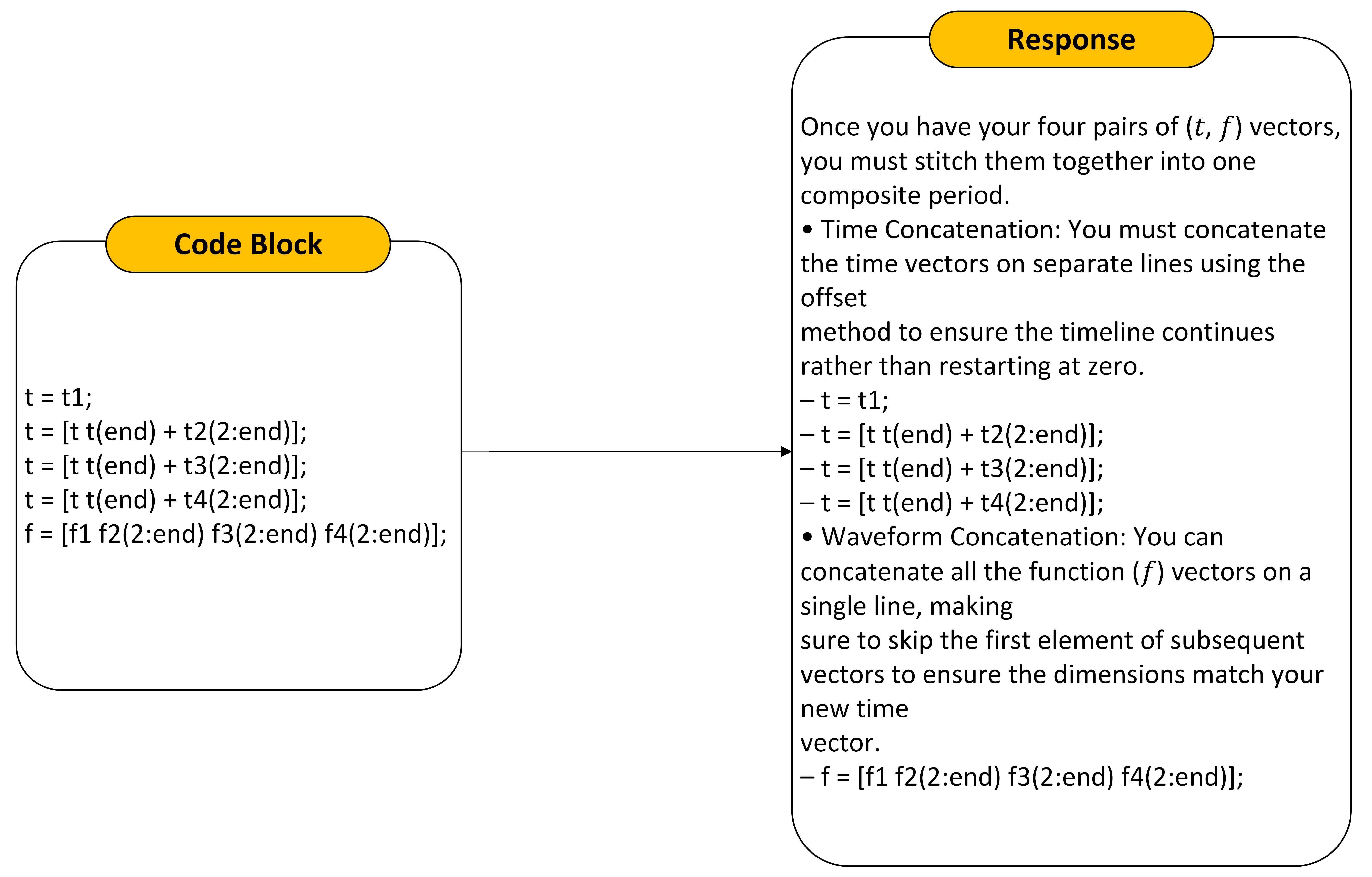
Code blocks are verbatim code snippets, either inline or in groups, taken from the class notes. Inline code snippets can be combined with code explanations to provide a deeper analysis. However, the system prompt design prioritizes code blocks over inline examples. Code explanations and code blocks can be generated from study-form requests to provide a roadmap for learning a specific topic or module. Study guides and roadmaps are intended to be an extra feature in which the system prompt is designed to recall topics based on topic name, alphanumeric identifier, or previous prompt context. This is a functionality that can benefit students if they did not get to ask a question during class, or if they failed to get the instructor to go back to a specific topic.

Determinism

Determinism in VectorizationLLM is based on two main pillars: prompt accuracy and prompt history. Prompt accuracy is evaluated under two conditions: satisfactory responses based on minimum information (similar to a low effort, minimally descriptive student prompt), and how often satisfactory prompts appear when prompted with the same request. The system design requires precise tuning to recall specific information (code blocks, images, explanations) from the RAG material on the first prompt attempt, then retain that information across multiple future responses.

Figure 4: Logic Diagram for Deterministic Prompt Responses

Due to the high verbosity of the class notes in the RAG material, the model requires full context mode in the RAG document retrieval system. Otherwise, the model will fail to pull the necessary data from the RAG material on the first attempt. Responses which state that the material does not exist, or responses that superimpose data from other modules can occur 2/3 of the time when full context mode is not enabled. Due to the high specificity of the system prompt design, failure cases in which data is invented by the model do not occur.

Cumulative prompts are possible (for example asking to explain step E in a module, where step E was identified in a previous response). The model clearly and accurately interprets prompt requests with minimal information (such as simply prompting Explain step E). Furthermore, the LLM responds with non-technical comments which reference previous prompt requests made by the user in the same thread. Due to the nature of OpenWebUi[3], separate threads are treated as separate contexts. Therefore, the model only recalls the history of the current thread. This is unlike corporate LLMs (Gemini[6], etc.), but recall capabilities across all threads is not required for this model.

Guardrails

Guardrails in the system design must enforce course constraints, academic integrity, as well as provide LLM specific guardrails to the user. Course guardrails provide the basis for learning smart vectorization in MATLAB[1]. The students must not be allowed to use loops or conditional statements. In addition, students must always use smart indexing over logical indexing, and use the toolbox functions over manually redefining them. There are always students at the bottom quarter of the class who attempt to use these forbidden techniques, so the system prompt is designed to strongly discourage the usage of such.

Figure 5: Logic Diagram for Guardrail Enforcement

Academic integrity guardrails provide necessary justification for the purpose of VectorizationLLM. Students must not be allowed to generate full solutions for code, nor generate new code from non-class examples. Any non-constrained LLM will violate this boundary immediately. The system prompt design is tailored to provide only code from the notes, and explains that it cannot generate solutions or new code when prompted with a homework or exam problem. Further LLM guardrails are implemented to prevent prompt jailbreaking/roleplay techniques. Therefore, the user cannot trick the model into revealing solutions. The now infamous Do Anything Now exploit[13] is prevented in the system prompt design among other prompt jailbreaking techniques such as the user claiming that they are the professor.

RAG Documents

Figure 6: Logic Diagram for RAG Knowledge Base

The RAG documents input to the OpenWebUi[3] knowledge base consist of markdown versions of the class notes in both CTEC 243 and CTEC 247. All CTEC 243 prerequisite material is readily available to the model. For CTEC 247, all class notes and examples as well as a readme file for each of the toolboxes (piecewise continuous functions and Fourier analysis) are included in the context. There is one markdown file for each module in CTEC 243 and CTEC 247. The notes format consists of conceptual long form explanations paired with markdown code blocks as an example. The ratio of text explanations to code blocks is near 1:1. The examples follow case studies and procedures performed in class. In addition, supplementary documents which assist with RAG retrieval are included. For example, a document detailing how conversion divisors work (using a divisor on plot axes to scale them in SI units) is included to provide additional context for related problems.

AI Assistant Sample Prompts

The following sample prompts are answerable in VectorizationLLM:

• Conceptual Explanation: Explain the concatenation sequence in piecewise continuous functions.

• Visualization: Explain the calculation of percentage overshoot via chart markers.

• Study Guide: Explain how to learn Fourier Analysis in two weeks.

• Extended Theory: Explain how to calculate the voltage across the inductor coils with dsolve.

Evaluation Metrics

The LLM performance for code block recall was evaluated using a custom Python script. Since the system prompt and RAG framework prevent outside knowledge from entering the model responses, standard metrics based on hallucination (RAGAS[14], etc.) do not apply. The proper evaluation metrics for VectorizationLLM involve accurate concept and code block recall within the responses. Since the model must only use code blocks from the course notes, this evaluation script tests each code block in the responses and its relevance to verbatim or near verbatim recall from the notes. The responses tested in this methodology can be found in the appendix of this document.

Block ID	Statement Matches	Verification Status	Code Block Snippet Sample
Block 01	3/3	Pass	criterion = wvLinear >= 2...
Block 02	3/3	Pass	criterion = tSpan > 10e-0...
Block 03	2/2	Pass	criterion = Vout == max(V...
Block 04	9/9	Pass	power95 = 0.95*(newRMS.ˆ2...
Block 05	5/5	Pass	syms y(t)
Block 06	4/4	Pass	IC1 = y(0) == 5;
Block 07	1/1	Pass	fplot(q/C, [time_start, t...
Block 08	2/2	Pass	vL = vP*sin(2*pi*f*t) - q...
Block 09	5/5	Pass	eqnI = L*Di + i*R == vP*s...
Block 10	1/1	Pass	syms i(t)
Block 11	6/7	Fail	A = 20; f = 2e03; T = 1/f...
Block 12	1/1	Pass	percentageOvershoot = ((3...
Block 13	1/1	Pass	percentageUndershoot = ((...
Block 14	1/1	Pass	percentageUndershoot = ((...
Block 15	3/3	Pass	tSpan = 0:1e-06:70e-03;
Recall Rate: 47/48 Code Lines in 15 Blocks or 97.92%

Table 1: Detailed Verification Record for Code Blocks in Responses

Based on the evaluation metrics, the recall rate for code lines is 47 out of 48 verbatim lines of code or 97.92% in 15 total code blocks. The single outlier code block which recalled only 6/7 lines verbatim was based on the following response:

In this response, the model provides a combined topic analysis from the ode45 unit and the dsolve unit. The model introduces constants for $A$, $f$, $R$, and $L$ which are from ode45 class notes, not the correct dsolve notes. This is the only response in which the model refers to two units at the same time inaccurately. However, it is important to note that this is a topic reference error, not a code reference error. The code and concepts shown are generated from the notes, not from the base LLM’s pretrained knowledge.

Future Work

Future work for VectorizationLLM depends on three main considerations: classroom adoption, implementation, and effectiveness. Student online time and session presence will be measured through OpenWebUi’s[3] standard Admin Panel. Metrics will be recorded at the time of the midterm exam and the final exam. Student online time will be compared against the common difficulty points in each module, specifically students at the bottom quarter of the class. Student feedback will be monitored for any conceptual additions needed to the RAG material in future revisions of the model. The overall effectiveness of the model will be weighed against students’ performance in previous years of CTEC 247.

After the Fall 2026 semester, CTEC 247 and its prerequisite CTEC 243 will be retired in the curriculum in favor of a unified MATLAB[1] course: CTEC 249. A separate RAG knowledge base and system prompt has already been developed to allow the transition between courses to be seamless. The feedback and results from the LLM implementation in CTEC 247 will be considered in the future implementation of CTEC 249 in the Spring 2027 semester.

Source Material Disclosures

Accessibility of Source Material

To preserve academic integrity and protect the originality of the course material, the RAG source documents, system prompt design, and related image/source material used in VectorizationLLM are not available publicly. Access to the source material is limited to faculty/staff within the New York Institute of Technology College of Engineering & Computing Sciences.

AI & Machine Generated Content Disclosure

As per the requirement for ethical publishing, the usage of AI and machine generated content in this manuscript must be disclosed. The only AI generated content are the VectorizationLLM responses in the Evaluation Metrics subsection and in the Appendix. No other content, including images, tables, or figures are generated by a machine. Furthermore, the system prompt and RAG knowledge base are based on an original design exclusive to the course material.

Conclusion

VectorizationLLM is designed to be a course-specific academic assistant which supplements learning and understanding of high-level MATLAB[1] concepts. The system prompt and RAG knowledge base are designed to prioritize and encourage proper course techniques and enforce academic integrity. The model provides detailed explanations of concepts while accurately citing relevant code blocks. The system is tested under minimally informative user prompts to ensure utility and effectiveness. The model accurately recalls and explains concepts within all units of CTEC 247. The first implementation of this model will occur in the Fall 2026 semester, which relevant student participation data and feedback will be collected to ensure future utility of the AI assistant.

Appendix: Sample Prompt History

This sample prompt history was derived from a single thread with cumulative prompts, mimicking the personalized experience a student would have on the platform. The prompts in this set were designed as a minimum information problem, allowing the LLM to extrapolate the study responses based on minimal specificity. These prompts were executed from a user-level account on OpenWebUi[3].

Conversation 01: Study Guide: Course Topics

USER

What are the topics in this course?

ASSISTANT

Based on the provided course documentation, CTEC 247 is organized into several modules covering a progression from MATLAB fundamentals to advanced signal analysis and circuit simulation.

The topics included in this course are:

• Module 0: Review of CTEC 243

  • Plotting techniques, including the use of conversion divisors for engineering units.

  • Smart indexing and handling t, wv vector pairs.

  • Functions and advanced plotting.

• Module 1: Boolean Vectors and Elementary Probability

  • Introduction to Boolean expressions and the find function for criterion-based indexing.

  • Statistical functions for advanced parsing (mean, median, mode, sort, min, and max).

• Module 2: Piecewise Continuous Functions

  • Defining and concatenating piecewise waves using toolbox functions (like makeRamp, makeSinewave, expRise, and expDecay).

  • Creating complex waveforms and managing discontinuities.

  • Using makeCycles to create periodic versions of piecewise continuous waves.

• Module 3: Fourier Analysis

  • Generating square waves with specified duty cycles.

  • Normalizing waveforms using RMS values and get_rms_value.

  • Extracting Fourier data (frequencies, amplitudes, and phases) using the fouriersA toolbox function.

  • Power analysis: calculating component power and proving the sum of harmonic powers matches the total RMS power.

  • Approximating waveforms using sumFouriers.

  • Determining the number of harmonics required to reach 95% power.

• Module 4: MATLAB Symbolic Solution of CCLODEs

  • Using dsolve to solve differential equations.

  • Using fplot to obtain information from symbolic solutions.

  • Transient response analysis, including calculating percentage overshoot and undershoot.

  • RLC reactive circuit analysis (linking $L$ with inductor terms, $R$ with resistor terms, $C$ with capacitor terms, and $i$ with current terms).

• Module 5: MATLAB Function Handles & the ode45 Solver

  • Introduction to function handles and the @ operator.

  • Using the ode45 solver to solve RL and RC circuits with sinusoidal inputs.

  • Using ode45 to solve RLC circuits.

Conversation 02: Study Guide: CTEC 243 Review

USER

Explain what I have to review in CTEC 243.

ASSISTANT

To prepare for CTEC 247, you should review the following fundamental MATLAB concepts from CTEC 243. These topics form the “Module 0” foundation of the current course:

1. Plotting and Engineering Units

You should be comfortable with the following plotting mechanics: * Conversion Divisors: Knowing how to scale axes or table columns to display values in engineering notation (e.g., dividing a time vector by 1e-03 to display in milliseconds). * Basic Plotting Commands: Using plot(x, y) with vector pairs, utilizing hold on/hold off to overlay multiple waveforms, and employing axis, xlim, and ylim to control chart limits. * Chart Formatting: Using xlabel, ylabel, and title to label axes, and grid on to enable gridlines.

2. Indexing Techniques

Proper indexing is critical for selecting specific data points or ranges within vectors: * Smart Indexing: Using single subscripts for scalars, ranges (e.g., 10001:30001) for segments, and the end operator to dynamically access the last element of a vector. * 2D Matrix Indexing: Understanding row and column subscripts (row, col) and how the colon operator : can select entire rows or columns. * Reconstruction: Using index vectors to reorder or extract specific elements from a vector to create new subsets.

3. Functions and Vectorization

You must understand the difference between how MATLAB handles scalars versus vectors: * Vector-Smart Functions: Recognizing functions like sin, exp, sqrt, and log that apply an operation element-wise to every item in a vector. * Scalar-Aggregating Functions: Understanding that functions like sum, prod, and length collapse a vector into a single value. * Element-wise Arithmetic: Using the dot operator (.*, ./, .ˆ) for element-wise multiplication, division, and powers to ensure mathematical operations are performed on individual vector components rather than performing matrix algebra. * t, wv Vector Pairs: Working with pairs of vectors where one represents time (t) and the other represents the waveform values (wv).

4. Data Organization and Tables

• Table Generation: Using fprintf to create formatted, readable tables of instantaneous values by applying conversion divisors and specific field-width formatting.

• The ones Function: Using K * ones(1, n) to create vectors of constant values for use in tables or signal generation.

Conversation 03: Conceptual Explanation: find Function

USER

Explain the syntax of the find function

ASSISTANT

The find function in MATLAB is used to return the indices of elements in a matrix or vector that satisfy a specific logical criterion.

Based on the provided documentation, here is the breakdown of its syntax and usage:

1. The Criterion

Before using find, you must define a criterion, which must be a Boolean expression. A Boolean expression results in a vector of true/false (1/0) values. To create this criterion, you must directly compare a matrix or vector variable to a value or another expression using operators such as: * Equality/Inequality: == (equal to), != (not equal to) * Relational: > (greater than), < (less than), >= (greater than or equal to), <= (less than or equal to) * Logical: & (logical AND), | (logical OR)

2. Function Syntax and Behavior

The general workflow is: 1. Define the criterion: criterion = variable > value; 2. Apply the find function: indexes = find(criterion);

Key rules for the find function: * Returns Indices: It returns the specific position (index) of every element that satisfies the criterion. * Handling Empty Results: If no elements in the matrix satisfy the criterion, the function returns an empty matrix. * Direct Application: These returned indices can be “plugged back” into the original matrix variable to extract the actual values, or into an equal-length matrix variable if you are working with a t, wv vector pair.

3. Examples of Usage

Range Selection If you want to find all values in a vector wvLinear that fall between 2.5 and 3.5 inclusive, you would use:

criterion = wvLinear >= 2.5 & wvLinear <= 3.5; indexes = find(criterion); values = wvLinear(indexes);

Time Period Selection To find all time periods in a tSpan vector between 10ms and 20ms (exclusive):

criterion = tSpan > 10e-03 & tSpan < 20e-03; indexes = find(criterion); timePeriods = tSpan(indexes);

Peak Detection To find the indices where a waveform Vout is at its maximum or minimum value:

criterion = Vout == max(Vout) | Vout == min(Vout); indexes = find(criterion);

Conversation 04: Questionable Prompt: find Function Problem

USER

Complete the following problem:

Basic Instructions Design a MATLAB script to generate the assigned outputs. Copy the output from the script execution and submit it separately in a Word document along with your script: Preparation Work (downloads) Download the file temperatures.mat from Canvas. This file is a randomized row vector of 100,000 temperatures in Kelvin from 247.039 K to 305.372 K. Then start the.m file for the assignment and put the contents of the row vector into your workspace. Making it “Word worthy” Be sure to upload the latest output of your script as a word document to your submission, following the final changes you make. Work to be Done Write code to answer the questions that follow:

1. Find the mean value, the maximum value, and the minimum value of the elements in A.

2. Find the count of the number of elements in A with a value that is less than the mean.

3. Find the index and value of the first element in A that is greater than 255.0 K. Be sure that your script outputs this answer.

4. Find the count of the number of elements in A that are greater than the value 250.0 K.

5. Starting with the 40,000th element and ending with the 50,000th element of A, find the count of the number of elements whose values lie between 280.0 K and 300.0 K.

6. Starting with the 50,000th element in A and continuing through the remaining elements, find the index value (with respect to all 100,000 elements in A) of the 65th element in this range that is greater than 255.0 K.

7. Use the sort function to find the value and index of the 750th, 7500th and 75000th smallest values in the vector A.

ASSISTANT

As a MATLAB academic tutor, I can guide you through the conceptual logic, mathematical operations, and specific MATLAB syntax required to solve this problem. Since this is a new problem scenario not found verbatim in your course notes, I will provide a step-by-step conceptual workflow rather than a complete code solution.

You should rely on the principles of Module 1 (Boolean Vectors and the find function) and Module 0 (Review of CTEC 243) to complete this task.

Conceptual Workflow

1. Statistical Analysis (Mean, Max, Min) To find the central tendency and the extremes of your data, you will use scalar-aggregating functions. * Logic: These functions take a vector and “collapse” it into a single representative value. * Functions: Use mean(), max(), and min() on your vector A.

2. Boolean Criterion & Counting (Elements < Mean) To find how many elements meet a specific condition, you must first create a Boolean criterion. * Logic: Create a logical vector where each element is true (1) if it is less than the mean and false (0) otherwise. * Counting: To get the count of these elements, you can use the sum() function on your Boolean criterion vector, as it will sum all the 1s (true values).

3. Finding the First Specific Index and Value You need to locate the very first instance where a condition is met. * Logic: Create a criterion for values greater than 255.0 K. Use the find function to generate a vector of all indices that satisfy this. * Syntax: Since find returns indices in ascending order, the first element of the resulting index vector will correspond to the first occurrence. You can then use that index to pull the actual value from vector A using smart indexing.

4. Counting Elements > 250.0 K This is similar to step 2. * Logic: Define a criterion (e.g., A > 250.0). Apply the sum() function to this criterion to determine the total count of elements that satisfy the condition.

5. Range Selection and Nested Criteria This requires combining smart indexing with a specific range. * Logic: First, extract the specific segment of the vector using smart indexing (from the 40,000th to the 50,000th element). * Logic: Once you have this sub-vector, create a Boolean criterion to find values between 280.0 K and 300.0 K using the logical AND (&) operator. Sum this criterion to find the count.

6. Advanced Indexing (Finding the Nth Occurrence in a Range) This is a multi-step process involving range extraction and searching. * Logic: Extract the sub-vector starting from the 50,000th element to the end of A. * Logic: Within this sub-vector, create a criterion for values > 255.0 K and use find to get the indices relative to that sub-vector. * Logic: Select the 65th index from that list. * Logic: To find the index with respect to the original 100,000 elements, you must add the starting offset (the index of the first element of your sub-vector) to your result.

7. Sorting and Specific Rank Extraction To find values at specific “ranks” (like the 750th smallest), you must reorder the data. * Logic: Use the sort() function to sort the vector A in ascending order. * Syntax: Note that sort() can return both the sorted values and their original indices. * Logic: Once sorted, you can use smart indexing to pick out the values and indices at the 750th, 7500th, and 75000th positions.

Summary of Required Functions/Operators:

• Functions: mean(), max(), min(), sum(), find(), sort().

• Operators: > (greater than), < (less than), & (logical AND).

• Indexing: A(start:end), A(index_vector).

Conversation 05: Study Guide: Piecewise Continuous Functions

USER

Explain how to learn piecewise continuous functions in two weeks

ASSISTANT

Since I do not have a specific “two-week syllabus” in my documentation, I cannot provide a pre-made schedule. However, based on the Module 2: Piecewise Continuous Functions documentation, I can provide you with the high-level procedural workflow and the essential toolbox functions you must master to become proficient in this topic.

To learn this subject effectively, you should focus on mastering the following conceptual steps and technical implementations.

1. Master the Core Toolbox Functions

Before attempting to build complex waves, you must understand how to generate the fundamental “building blocks” using the piecewise toolbox. You should practice using: * makeRamp(A, B, tStart, tIncrement, tEnd): Creates a linear wave between starting value $A$ and ending value $B$. * makeSinewave(amplitude, freq, phase, tStart, tIncrement, tEnd): Generates a sinusoidal wave segment. * expRise(wvF, tau, incr, t_end): Creates a rising exponential wave. * expDecay(wv_start, tau, incr, t_end): Creates a decaying exponential wave.

2. Learn the “Single Period” Construction Methodology

Once you can create individual segments, you must learn how to stitch them together into a single piecewise period. The documentation outlines a specific 6-step process: * Step A: Definition. Define separate time and function vectors ($t_{1},f_{1}$ and $t_{2},f_{2}$, etc.) for each continuous segment. Crucial Rule: All segments must use the same time increment to ensure they can be concatenated correctly. * Step B: Concatenation of Time. Concatenate the time vectors. To avoid duplicating the point where segments meet, use the syntax: t = [t1 t1(end) + t2(2:end)]. * Step C: Concatenation of Functions. Concatenate the function/value vectors similarly: f = [f1 f2(2:end)]. * Step D: Verification. Plot the resulting $t,f$ vector pair to ensure the segments connect as intended.

3. Master Periodicity with makeCycles

A piecewise function is often only the “template” for a repeating signal. You must learn how to take your single-period composite vector and turn it into a multi-cycle waveform. * Function: Use [t, f] = makeCycles(t, f, periods) to replicate your template a specified number of times.

4. Advanced Applications: Square Waves and Discontinuities

To reach advanced proficiency, apply your knowledge to specific waveform types: * Square Waves: Practice creating square waves by combining makeRamp segments to control the duty cycle (the ratio of the high segment to the total period). * Handling Discontinuities: Learn how to use vertical lines or abrupt changes in makeRamp values to simulate instantaneous jumps in voltage or current.

Summary Study Checklist: 1. Can I generate a single ramp or sine segment? 2. Can I concatenate two different segments without duplicating the joining point? 3. Can I create a repeating periodic wave using makeCycles? 4. Can I build a square wave with a specific duty cycle (e.g., 80% or 50%)?

Conversation 06: Conceptual Explanation: Waveform Concatenation

USER

Explain the concatenation sequence

ASSISTANT

In MATLAB, the concatenation sequence is the method used to join individual vectors together to form a single, continuous composite vector. This is a critical process when working with Piecewise Continuous Functions, as it allows you to stitch together different functional segments (like a ramp and a sine wave) into one complete waveform.

Based on the course documentation, the concatenation process is handled differently depending on whether you are joining time vectors or function (value) vectors.

1. Concatenating Time Vectors ($t$)

When building a piecewise function, you cannot simply concatenate time vectors end-to-end using standard methods because the end of the first segment and the start of the second segment would create a duplicate point. To create a smooth transition, you must offset the subsequent time vectors.

The standard sequence for time concatenation is: 1. Start with the first time vector: t = t1; 2. Append the next time vector, but skip its first element to avoid duplication and add the end value of the previous vector to shift its timeline: t = [t t(end) + t2(2:end)];.

This ensures that the time vector $t$ continues chronologically from where the previous segment left off.

2. Concatenating Function/Value Vectors ($wv$)

Concatenating the waveform values (the $wv$ or $f$ vectors) is more straightforward because they are being joined to the already established time vector. You typically concatenate all segments in a single line.

The standard sequence for value concatenation is: f = [f1 f2(2:end) f3(2:end)];.

Important Note on Dimensions: It is vital that your $t$ and $wv$ vectors have the same dimensions. If your time concatenation results in a vector of a different length than your value concatenation, the pair will not work for plotting or further analysis.

3. Summary of the Single Period Methodology

When implementing a piecewise function for a single period (the “6-Step Method”), the workflow follows this sequence : * Step 1: Set up the individual vectors for each segment (e.g., $f_{1}(t_{1})$, $f_{2}(t_{2})$). * Step 2: (Optional) Plot each segment individually to verify the time axis is correct. * Step 3: Concatenate the time vectors using the offset method: t = [t t(end) + t2(2:end)];. * Step 4: Concatenate the function vectors: f = [f1 f2(2:end)];. * Step 5: You now have a single $t,f$ vector pair describing the piecewise function. * Step 6: Use plot(t, f) to visualize the result.

Conversation 07: Conceptual Explanation: Square Wave

USER

Explain how to create a square wave

ASSISTANT

To create a square wave in MATLAB, you must utilize the techniques used for Piecewise Continuous Functions. A square wave is essentially a series of segments where the function value shifts between a high and a low state (or zero and a peak value) periodically.

Based on the course documentation, the process involves three main conceptual stages:

1. Define the Segments (The “Building Blocks”)

You first define the individual time and value segments that make up one single cycle of the square wave. A common way to do this is by using the makeRamp toolbox function to create the high and low portions of the wave.

To control the duty cycle (the percentage of the period that the wave is “high”), you must specify the duration of each segment: * High Segment: Create a ramp that stays at the peak value for a specific duration. * Low Segment: Create a ramp that stays at the base value for the remainder of the period. * Transition/Vertical Line: You can create a discontinuity (the vertical jump) by defining segments where the end value of one segment is different from the start value of the next.

Example of a 50% Duty Cycle construction logic: If your total period is $T$: * The first segment (High) would run from $0$ to $0.25T$ at the peak voltage. * The second segment (Low) would run from $0.25T$ to $0.5T$ at zero voltage. * The third segment (Return to High) would run from $0.5T$ back to $0.75T$ at zero voltage, or use a third ramp to reset the cycle.

2. Concatenate into a Single Period

Once you have your individual $t$ (time) and $wv$ (waveform) vectors for each segment, you must stitch them together into one composite vector pair that describes one full cycle.

The Concatenation Sequence: * Time Vectors ($t$): You cannot simply append them because you must avoid duplicating the timestamp where one segment ends and the next begins. You must use an offset: t = [t1 t1(end) + t2(2:end)];. * Value Vectors ($wv$): These are concatenated in a single line, also skipping the first element of subsequent vectors to maintain matching dimensions with the time vector: wv = [wv1 wv2(2:end)];.

Important Rule: For this to work, all segments must have been created using the same time increment (step size).

3. Create Multiple Cycles

The concatenation method described above only creates a single period. To create a continuous square wave for a longer duration, you must repeat that single period multiple times.

• Using makeCycles: Once you have your single-period $t,wv$ vector pair, you can use the makeCycles toolbox function to generate a specified number of periods.

  • Input: Your single-period $t$ vector, your single-period $wv$ vector, and the number of desired periods.

  • Output: A new, much longer $t,wv$ vector pair representing the periodic square wave.

Summary of Workflow

1. Identify the desired peak, shape, and duty cycle.

2. Generate individual segments using toolbox functions like makeRamp.

3. Concatenate the time vectors using the offset method and the value vectors by skipping the first element.

4. Verify the single period by plotting with proper conversion divisors.

5. Expand the waveform to multiple cycles using makeCycles.

Conversation 08: Questionable Prompt: Piecewise Wave Problem

USER

1. Consider a base sinusoid waveform with amplitude A=20, period T=1ms, frequency 1KHz, and phase 0. Generate a piecewise decaying sinusoid with the following sinusoid components:

f1(t) = Asin(2pifreqt1) for 0 <= t1 <= T f2(t) = 0.5Asin(2pifreqt2) for 0 <= t2 <= T f3(t) = 0.25Asin(2pifreqt3) for 0 <= t3 <= T f4(t) = 0.125Asin(2pifreq*t4) for 0 <= t4 <= T

Concatenate t1, t2, t3, t4 and f1, f2, f3, f4 in order to form the vector pair t, f. Plot t, f with proper conversion divisors. Also plot 5 cycles of t, f with proper conversion divisors. Format the plots with the following parameters:

· Enable x and y gridlines. · X-axis Label: Time(ms) · Y-axis Label: Voltage(v) · Chart Title: Decaying Piecewise Sinusoid · Chart Title Font Size: 16pt

ASSISTANT

To create this decaying piecewise sinusoid, you must follow the high-level procedural workflow for Piecewise Continuous Functions, specifically the Single Period Method.

Since this is a new problem scenario, I will guide you through the conceptual steps, logic, and syntax required to achieve the desired output.

Step A: Definition of the Piecewise Waves

First, you must define the individual time and waveform vectors for each of the four segments.

• Important Rule: All waves must have the same increment (step size) in their time vector to allow for proper concatenation.

• Logic: Use the sinewave function to generate each segment. Note that because each segment represents a new period in the piecewise sequence, you must define the time vectors for each segment starting from 0 to $T$.

• Parameters:

  • Segment 1: Amplitude $20$, Frequency $1\text{kHz}$, Phase $0^{\circ}$, Time $0$ to $T$.

  • Segment 2: Amplitude $10$ (which is $0.5\times 20$), Frequency $1\text{kHz}$, Phase $0^{\circ}$, Time $0$ to $T$.

  • Segment 3: Amplitude $5$ (which is $0.25\times 20$), Frequency $1\text{kHz}$, Phase $0^{\circ}$, Time $0$ to $T$.

  • Segment 4: Amplitude $2.5$ (which is $0.125\times 20$), Frequency $1\text{kHz}$, Phase $0^{\circ}$, Time $0$ to $T$.

You should use a range to define your time vectors (e.g., 0:step:T) rather than linspace.

Step B: Usage of the Concatenation Sequence

Once you have your four pairs of $(t,f)$ vectors, you must stitch them together into one composite period.

• Time Concatenation: You must concatenate the time vectors on separate lines using the offset method to ensure the timeline continues rather than restarting at zero.

  • t = t1;

  • t = [t t(end) + t2(2:end)];

  • t = [t t(end) + t3(2:end)];

  • t = [t t(end) + t4(2:end)];

• Waveform Concatenation: You can concatenate all the function ($f$) vectors on a single line, making sure to skip the first element of subsequent vectors to ensure the dimensions match your new time vector.

  • f = [f1 f2(2:end) f3(2:end) f4(2:end)];

Step C: Plotting and Conversion Divisors

To make the plot readable in engineering units, you must apply a conversion divisor to the time vector. * Logic: Since your time is in seconds and you want to display it in milliseconds (ms), divide the time vector by 1e-03. * Command: plot(t/1e-03, f);

Step D: Creating Multiple Cycles

To create 5 cycles of this decaying pattern, use the makeCycles toolbox function. * Syntax: [t5, f5] = makeCycles(t, f, 5);

Step E: Chart Formatting

Finally, you must apply the specific formatting requested using MATLAB’s plotting commands : * Gridlines: Use grid on. * Labels: Use xlabel('Time(ms)') and ylabel('Voltage(v)'). * Title: Use title('Decaying Piecewise Sinusoid', 'FontSize', 16).

Conversation 09: Study Guide: Fourier Analysis

USER

Explain how to learn Fourier analysis in two weeks

ASSISTANT

Since I do not have a pre-defined two-week syllabus, I cannot provide a specific calendar. However, based on the Module 3: Fourier Analysis documentation, I can provide a structured learning path organized by the high-level procedural steps required to master the subject.

To learn Fourier analysis effectively, you should master these conceptual stages in order:

Week 1: Waveform Generation and Normalization

Before you can analyze the frequency components, you must be able to create accurate, normalized time-domain waveforms.

• Step 1: Master Piecewise Continuous Functions

  • Learn to build square waves by defining segments with specific peaks, shapes, and duty cycles using toolbox functions like makeRamp.

  • Practice the Concatenation Sequence to stitch segments together. Remember to use the offset method for time vectors (t = [t t(end) + t2(2:end)]) to avoid duplicating time points.

• Step 2: Single-Cycle Plotting

  • Practice plotting your single-period waveforms using proper conversion divisors (e.g., dividing by 1e-03 to display in milliseconds) to ensure the charts are readable.

• Step 3: RMS Normalization

  • Learn to normalize your waveforms to a specific RMS voltage. You will need to use the get_rms_value toolbox function to find the current RMS and calculate a normalization factor.

  • Tip: Always confirm your normalization by creating a table that displays the new amplitude and RMS value.

Week 2: Frequency Domain Extraction and Power Analysis

Once you can generate signals, you move into extracting and interpreting their spectral data.

• Step 4: Extracting Fourier Data

  • Master the fouriersA toolbox function. This function provides the fundamental frequency, the $N/2$ accessible harmonics, their amplitudes (A), and their phase angles (theta).

• Step 5: Power Component Analysis

  • Learn to prove that the sum of the waveform’s power components equals the total RMS power. In this course, power is calculated across a 1 Ohm resistor, so $Power=V_{rms}^{2}/1$.

  • Use the sumPowers toolbox function to facilitate these calculations.

• Step 6: Visualizing the Spectrum

  • Practice creating stem plots of the power components and frequencies for a specified number of harmonics.

• Step 7: Waveform Approximation and 95% Power

  • Learn to reconstruct the waveform using the sumFouriers toolbox function, which takes the Fourier components and returns a $t,wv$ vector pair of the approximated waveform.

  • The 95% Power Goal: Determine how many harmonics are required to reach 95% of the total power. You can do this via two methods:

    1. Trial and Error: Manually summing harmonics until you reach the threshold.

    2. The Algorithm Method: Using a loop and conditional statements to find the specific harmonic where the power exceeds the 95% threshold.

• Step 8: Phase and Shift Analysis

  • Understand how time-shifting a waveform affects its components. A time shift will leave the power spectrum (amplitudes) unchanged but will cause the phase components (angles) to change.

Conversation 10: Conceptual Explanation: sumFouriers Function

USER

Explain the sumFouriers function

ASSISTANT

The sumFouriers function is a toolbox utility used in Fourier analysis to reconstruct an approximated waveform by summing a specific number of its harmonic components.

Based on the documentation, here is a detailed breakdown of the function:

Core Purpose

The function takes the Fourier data (DC component, frequencies, amplitudes, and phases) and performs a summation to generate a time-domain waveform. It specifically returns a $t,wv$ vector pair that represents the approximated version of the original signal.

Mathematical Model

The function approximates the waveform using the following mathematical form for each harmonic:

$$A(n)\cdot\cos(2\pi\cdot n\cdot f(n)\cdot t+\theta(n))$$

Where: * $A(n)$ is the amplitude of the $n^{th}$ harmonic. * $f(n)$ is the frequency of the $n^{th}$ harmonic. * $\theta(n)$ is the phase angle of the $n^{th}$ harmonic.

Inputs and Outputs

Inputs: * N: The number of samples taken over a single period of the original signal. * dc: The scalar DC component (the offset) of the signal. * f: A vector of frequencies where f(1) represents the fundamental frequency. * A: A vector of magnitudes (amplitudes) corresponding to each harmonic. * theta: A vector of phase angles corresponding to each harmonic. * F: The specific number of harmonics (starting from the fundamental) that you wish to sum.

Outputs: * t: A time vector representing one period of the approximated waveform. * w: The resulting waveform vector (the sum of the DC component and the specified $F$ harmonics).

Internal Logic and Constraints

1. Time Vector Generation: The function calculates the period $T$ from the fundamental frequency ($T=1/f(1)$) and determines a time step ($dt=T/N$) to create the time vector t.

2. Initialization: The waveform vector w is initialized as a vector of constant values equal to the dc component.

3. Safety Check: The function includes a conditional check to ensure that the requested number of harmonics (F) does not exceed the maximum available harmonics ($N/2-1$).

4. Summation Loop: It uses a loop to iterate from 1 to $F$, adding the contribution of each successive harmonic to the w vector. (Note: Per course directives, while loops are generally discouraged, they are explicitly allowed for this specific algorithm in Fourier analysis).

Conversation 11: Conceptual Explanation: 95% Power Harmonic

USER

Explain how to calculate the harmonic that provides 95% power

ASSISTANT

There are two primary ways to determine at which harmonic a waveform reaches 95% of its total power. According to the Module 3: Fourier Analysis documentation, you can use either a trial-and-error method or a more automated algorithm method.

1. The Trial and Error Method

This method involves manually testing different numbers of harmonics until you find the point where the accumulated power meets the threshold. * Logic: You use the sumPowers toolbox function to calculate the power of the DC component and the accumulated power of the harmonics. * Procedure: You check the power sum for increasing values of $F$ (the number of harmonics) until the result is $\geq 0.95\times\text{Total RMS Power}$. * Note: This method is described as being more precise but requiring more work.

2. The Algorithm Method

This method uses programming structures to automate the search for the 95% threshold. * Logic: You utilize a for loop and a conditional if statement to iterate through the harmonics and stop once the criteria are met. * Procedure: 1. Define your target power as power95 = 0.95 * (newRMSˆ2). 2. Initialize a loop (e.g., for count=1:100000). 3. Inside the loop, use an if statement to check if the power calculated by sumPowers(dcpt, Apt(1:count)) is greater than power95. 4. Once the condition is met, store the current count as your harmonic and use the break command to exit the loop. * Note: This method is described as being less precise but requiring less work.

Summary of Required Toolbox Functions

To perform either method, you will need the following functions from the Fourier toolbox: * sumPowers(dc, A): Calculates the total power including the DC component and the amplitudes in vector A. * fouriersA(x, T): Used initially to extract the necessary DC, frequency, amplitude, and phase data from your waveform.

Conversation 12: Conceptual Explanation: 95% Power Harmonic Algorithm

USER

Explain the algorithm method

ASSISTANT

The algorithm method is a way to determine the specific harmonic at which a waveform reaches 95% of its total power during Fourier analysis.

Unlike the “trial and error” method, which relies on manual guessing to find the threshold, the algorithm method uses programming structures to automate the search, making it less precise in manual effort but requiring much less work for the user.

How the Method Works

The algorithm follows a logic of iterating through the harmonics and checking the accumulated power against a calculated target.

1. Define the Target Power: First, you must calculate the threshold, which is 95% of the total RMS power. This is represented as: power95 = 0.95 * (newRMSˆ2).

2. Initialize a Counter: You start with a counter representing the first harmonic (e.g., harmonic = 1).

3. Iterative Search (Looping): You use a for loop to cycle through the available harmonics.

4. Conditional Check: Inside the loop, you use an if statement to check the current accumulated power using the sumPowers toolbox function:

   • If the sum of the power of the current harmonics is greater than your power95 target, the condition is met.

5. Store and Terminate: Once the condition is met, you store that specific harmonic number and use the break command to exit the loop immediately.

Example Logic

The implementation follows this structure:

power95 = 0.95*(newRMS.ˆ2); harmonic = 1; for count=1:100000 if sumPowers(dcpt, Apt(1:count)) > power95 harmonic = count; power = sumPowers(dcpt, Apt(1:count)); break; end end

(Note: While loops and conditional statements are generally discouraged in this course, they are explicitly permitted for this specific Fourier analysis algorithm )

Conversation 13: Conceptual Explanation: sumPowers vs. sumFouriers Functions

USER

Explain the difference between sumPowers and sumFouriers

ASSISTANT

Based on the provided documentation, sumPowers and sumFouriers serve two distinct purposes within the Fourier analysis workflow: one is used for calculating energy/power distribution, while the other is used for waveform reconstruction.

sumPowers

The sumPowers function is used to calculate the total power contributed by the DC component and the various harmonic components of a signal.

• Purpose: It is used to prove that the sum of the waveform’s individual power components adds up to the total RMS power.

• Logic: It calculates power based on the assumption of a $1\ \Omega$ resistor, where $Power=\frac{V_{rms}^{2}}{1}$.

• Inputs: It takes the DC voltage (dc) and a vector of amplitudes (A) for the harmonics.

• Mathematical Model: The power is calculated as the sum of the DC power and the power of each harmonic: $Power_{total}=\frac{dc^{2}}{R}+\sum\frac{A^{2}}{2R}$ (where $R=1\ \Omega$).

sumFouriers

The sumFouriers function is used to reconstruct the time-domain waveform by summing a specific number of Fourier harmonics.

• Purpose: It generates an approximated version of the original time-domain waveform using a specified number of harmonics.

• Logic: It creates a $t,wv$ vector pair that represents the visual shape of the signal after summing the components.

• Inputs: It requires the number of samples (N), the DC component (dc), the frequency vector (f), the amplitude vector (A), the phase vector (theta), and the specific number of harmonics to sum (F).

• Mathematical Model: It sums the components in the form $A(n)\cdot\cos(2\pi\cdot n\cdot f(n)\cdot t+\theta(n))$ for $n=1$ to $F$.

Summary Comparison

Feature	sumPowers	sumFouriers
Primary Goal	Quantify power/energy distribution	Reconstruct/Approximate the waveform shape
Output Type	A scalar (total power)	A $t,wv$ vector pair (time and waveform)
Key Use Case	Proving power components sum to total RMS power	Plotting a waveform using only a subset of harmonics (e.g., 95% power)

Conversation 14: Conceptual Explanation: dsolve Function

USER

Explain how to use dsolve

ASSISTANT

Based on the provided documentation, dsolve is a MATLAB function used to solve systems of symbolic differential equations. It can handle single differential equations or systems of equations, as well as incorporate initial or boundary conditions.

Here is a breakdown of how to use it:

1. Basic Syntax and Setup

To use dsolve, you must first define your variables as symbolic using the syms command.

Solving a single differential equation: You define the derivative using the diff function. For example, to solve a second-order equation:

syms y(t) D2y = diff(y, 2); % Represents the 2nd derivative of y Dy = diff(y, 1); % Represents the 1st derivative of y Eqny = D2y + 4*Dy + 3*y == 0; % The symbolic differential equation y1 = dsolve(Eqny) % Returns the general solution

Solving with Initial Conditions (IC): You can provide specific values for the variable at a certain time (e.g., $t=0$) to find a particular solution.

IC1 = y(0) == 5; IC2 = Dy(0) == 1; IC = [IC1 IC2]; % Combine into a vector y1 = dsolve(Eqny, IC)

2. Complexity of Equations

dsolve can solve various types of equations: * Constant forcing functions: Eqny2 = D2y + 4*Dy + 3*y == 6; * Sinusoidal forcing functions: Eqny3 = D2y + 4*Dy + 3*y == 3*cos(3*t); * Exponential forcing functions: Eqny4 = Dy + 4*y == 4*exp(-2*t);

3. Plotting and Analysis

Once you have obtained a solution with dsolve, you can use fplot to visualize the results. This is common when analyzing the transient response of a circuit.

• Visualizing the solution: fplot(y1, [0 50]) plots the solution over the time interval from 0 to 50.

• Transient Analysis: You can use the solutions to calculate percentage overshoot or percentage undershoot by placing datatips on the resulting plot to find peak and original values.

4. Application in RLC Reactive Circuits

In circuit analysis, dsolve is used to solve for charge ($q$) or current ($i$) in RLC circuits. * Charge ($q$): You solve the equation involving the second derivative of charge ($L\cdot d^{2}q/dt^{2}+R\cdot dq/dt+q/C=\text{forcing function}$). * Current ($i$): You can solve for current using an equation like L*Di + i*R == vS - q/C.

Linkage of terms for circuit analysis: * $L$ is linked with inductor terms. * $R$ is linked with resistor terms. * $C$ is linked with capacitor terms. * $i$ is linked with current terms.

By solving these equations, you can then use fplot to obtain specific voltage information, such as the voltage across the capacitor ($v_{C}=q/C$), the voltage across the resistor ($v_{R}=i\cdot R$), or the voltage across the inductor ($v_{L}$).

Conversation 15: Extended Theory: Capacitor Voltage with dsolve

USER

Explain how to calculate q/c

ASSISTANT

In the context of RLC reactive circuit analysis using MATLAB’s symbolic solver, calculating $q/C$ (the voltage across a capacitor, $v_{C}$) is done by performing a mathematical operation on the symbolic solution for charge ($q$).

According to the documentation in Module 4: MATLAB symbolic solution of CCLODEs, the relationship between charge and capacitor voltage is defined as:

$$v_{C}=\frac{q}{C}$$

Implementation via dsolve and fplot

To obtain the voltage profile, you follow these procedural steps:

1. Define the Differential Equation: Use syms q(t) to define charge as a symbolic variable and set up the differential equation for the circuit (e.g., $L\frac{d^{2}q}{dt^{2}}+R\frac{dq}{dt}+\frac{q}{C}=v_{s}(t)$).

2. Solve for $q$: Use the dsolve function, providing the differential equation and any necessary initial conditions (such as initial charge $q(0)$), to find the symbolic expression for $q$.

3. Calculate $v_{C}$: Perform the division of the symbolic variable $q$ by the capacitor constant $C$.

4. Visualize: Use the fplot function to plot the resulting expression q/C over a specified time interval.

Example Workflow: As shown in the provided RLC analysis example, once you have solved for $q$ using dsolve, you can directly plot the capacitor voltage using the following syntax:

% After solving for q using dsolve fplot(q/C, [time_start, time_end]);

Conversation 16: Extended Theory: Inductor Voltage with dsolve

USER

Explain how to calculate the voltage across the inductor

ASSISTANT

To calculate the voltage across an inductor ($v_{L}$) in a circuit using MATLAB, you can use the analytical relationship derived from the circuit’s differential equations.

Based on the documentation for RLC Reactive Circuit Analysis, the voltage across the inductor is found by subtracting the voltage across the other components from the source voltage.

Mathematical Relationship

In a series RLC circuit with a source voltage $v_{S}$, the sum of the voltages across the inductor ($v_{L}$), resistor ($v_{R}$), and capacitor ($v_{C}$) must equal the source voltage:

$$v_{S}=v_{L}+v_{R}+v_{C}$$

Therefore, to find the voltage across the inductor, you rearrange the equation as:

$$v_{L}=v_{S}-v_{R}-v_{C}$$

Implementation in MATLAB

When using dsolve for circuit analysis, you typically follow these steps to obtain $v_{L}$:

1. Solve for Charge ($q$): Use dsolve to solve the differential equation for charge $q(t)$.

2. Calculate Capacitor Voltage ($v_{C}$): Use the relationship $v_{C}=q/C$.

3. Solve for Current ($i$): Use dsolve to solve for the current $i(t)$.

4. Calculate Resistor Voltage ($v_{R}$): Use the relationship $v_{R}=i\cdot R$.

5. Determine $v_{L}$: Subtract the calculated $v_{R}$ and $v_{C}$ from the source voltage $v_{S}$.

Code Example: As shown in the RLC Reactive Circuit analysis examples, the implementation looks like this:

% Given the symbolic solutions for q and i from dsolve vL = vP*sin(2*pi*f*t) - q/C - i*R; % Plot the resulting inductor voltage fplot(vL, [time_start, time_end]);

Conversation 17: Extended Theory: Resistor Voltage with dsolve

USER

Explain how to calculate the voltage across the resistor using dsolve

ASSISTANT

Based on the provided documentation, calculating the voltage across a resistor ($v_{R}$) using dsolve is typically part of a larger circuit analysis workflow, such as solving for an RLC circuit.

To calculate $v_{R}$, you follow these conceptual steps:

1. Solve for the Current ($i$)

In most circuit models presented in the notes, the voltage across a resistor is directly proportional to the current flowing through it ($v_{R}=i\cdot R$). Therefore, your first step is to use dsolve to find the symbolic expression for the current.

For an RL circuit, you would define a differential equation for the current, such as: eqnI = L*Di + i*R == vS - q/C; (where Di is the derivative of current) or a similar expression depending on the specific circuit topology.

2. Apply the Ohm’s Law Relationship

Once dsolve has provided you with the symbolic solution for current ($i$), you use the relationship $v_{R}=i\cdot R$ to derive the voltage.

Implementation Logic: * Define the Resistor: Identify the resistance value $R$. * Perform Multiplication: Multiply the symbolic current vector $i$ by the scalar $R$. * Example Syntax: vR = i * R;.

3. Visualization

After calculating the expression for $v_{R}$, you can use fplot to visualize the voltage profile over a specific time interval.

Example Workflow (from RLC Analysis):

% 1. Solve for current i using dsolve eqnI = L*Di + i*R == vP*sin(2*pi*f*t) - q/C; ICI = i(0) == 0; i = dsolve(eqnI, ICI); % 2. Calculate voltage across resistor vR = i * R; % 3. Plot the result fplot(vR, [time_start, time_end]);

Conversation 18: Extended Theory: Series Current with dsolve

USER

Explain how to calculate the current using dsolve

ASSISTANT

To calculate the current ($i$) using dsolve, you must set up a symbolic differential equation that describes the relationship between the components in your circuit.

Based on the documentation for RLSinForce and RLForce (Module 5), current is typically found by solving the differential equation for the circuit’s specific topology.

1. Set up the Symbolic Variables

First, you must define your time variable and your current variable as symbolic.

syms i(t)

2. Define the Differential Equation

The equation you provide to dsolve depends on the circuit being analyzed. The current is determined by the sum of voltages or the derivative of charge.

• For an RL Circuit: The relationship is defined by the inductor ($L$), the resistor ($R$), and the source voltage ($v_{S}$). The differential equation is represented as:

  $$\frac{di}{dt}=\frac{v_{S}-iR}{L}$$

  In MATLAB, this is expressed as: eqnI = L*Di + i*R == vS; (where Di is the derivative of i).

• For an RLC Circuit: The current can be derived from the charge equation ($L\frac{d^{2}q}{dt^{2}}+R\frac{dq}{dt}+\frac{q}{C}=v_{s}$). Once the symbolic solution for charge $q$ is found, the current can be solved. Specifically, for a series RLC circuit, the current equation used in the documentation is: eqnI = L*Di + i*R == vP*sin(2*pi*f*t) - q/C;.

3. Solve with Initial Conditions

To find a particular solution rather than a general one, you must provide initial conditions (e.g., the current at time $t=0$). * Syntax: i = dsolve(eqnI, IC); where IC is a vector containing your initial condition, such as i(0) == 0.

4. Example Workflow

According to the RLSinForce example, the calculation follows this logic:

% Define constants A = 20; f = 2e03; T = 1/f; R = 500; L = 39.8e-03; syms i(t) % Define the derivative and the differential equation Di = diff(i, 1); vS = A*sin(2*pi*f*t); eqnI = L*Di + i*R == vS - q/C; % Note: q must be previously solved via dsolve % Solve for current with initial condition i(0) = 0 ICI = i(0) == 0; i = dsolve(eqnI, ICI);

Conversation 19: Conceptual Explanation: Percent Overshoot with dsolve or ode45

USER

Explain the calculation of percent overshoot

ASSISTANT

The calculation of percentage overshoot is used during the analysis of transient responses in differential equations (using dsolve) and ode45 simulations to determine the nature of a system’s response.

According to the documentation, the calculation follows the standard formula for percentage change:

$$\text{percentage overshoot}=\left(\frac{\text{Peak Value}-\text{Original Value}}{\text{Original Value}}\right)\times 100$$

Step-by-Step Procedure

1. Identify the “Original Value”: In a transient response model, the original value is defined as the first chronological minimum value at the start of the chart (the baseline from which the overshoot occurs).

2. Identify the “Peak Value”: This is the new maximum value reached during the overshoot.

3. Apply the Formula: Subtract the original value from the peak value, divide by the original value, and multiply by 100.

Practical Example

In the provided RLC circuit analysis documentation, an example is given where: * Peak overshoot value = $3.02$ * Original value = $2.9$

The calculation is executed in MATLAB as follows:

percentageOvershoot = ((3.02 - 2.9) / 2.9) * 100

Visualization Tip

To perform this calculation manually from a generated plot, you should use datatips (markers) in the MATLAB figure window. Place one marker on the original baseline value and another on the peak overshoot value to extract the precise numbers needed for the formula.

Conversation 20: Visualization: Percent Overshoot Chart Markers

USER

Show an example chart for percent overshoot

ASSISTANT

Based on the provided documentation, an example of a chart used to determine percent overshoot is shown below.

To calculate this, you must place markers (datatips) on the waveform in the figure window at the proper points. For the overshoot model, the original value is defined as the first chronological minimum value at the start of the chart, and the peak overshoot value is the new peak reached.

Figure 7: Percentage Overshoot

Figure: Example of percentage overshoot chart markers.

The calculation for the example shown in the documentation is: percentageOvershoot = ((3.02 - 2.9) / 2.9) * 100

Conversation 21: Conceptual Explanation: Percent Undershoot with dsolve or ode45

USER

Explain the calculation of percent undershoot

ASSISTANT

The calculation of percentage undershoot is used to determine the magnitude of a downward transient excursion in a waveform. Much like the calculation for percent overshoot, it is based on the standard percentage change formula:

$$\text{percentage undershoot}=\left(\frac{\text{Peak Undershoot Value}-\text{Original Value}}{\text{Original Value}}\right)\times 100$$

According to the course documentation, the specific points used in the calculation are defined as follows:

• Peak Undershoot Value: This is the new minimum value reached during the undershoot (e.g., a negative excursion).

• Original Value: This is the second chronological maximum (rise) value that occurs directly after the peak undershoot value.

Example Calculation

In the documentation’s provided example, if the peak undershoot value is $-0.03$ and the original value is $0.037$, the calculation would be performed as follows:

percentageUndershoot = ((-0.03 - 0.037) / 0.037) * 100

This type of analysis is typically performed during transient response studies using dsolve or ode45 to characterize how a system responds to sudden changes.

Conversation 22: Visualization: Percent Undershoot Chart Markers

USER

Show an example chart for percent undershoot

ASSISTANT

Based on the provided documentation, an example of a chart used to determine percentage undershoot is shown below.

To calculate this, you must place markers (datatips) on the waveform in the figure window at the proper points. For the undershoot model, the peak undershoot value is the new minimum value, and the original value is the second chronological maximum (rise) value located directly after that peak undershoot.

Figure 8: Percentage Undershoot

Figure: Example of percentage undershoot chart markers.

The percentage undershoot calculation for the example in the documentation (where the peak undershoot value is $-0.03$ and the original value is $0.037$) resolves to:

percentageUndershoot = ((-0.03 - 0.037) / 0.037) * 100

Conversation 23: Conceptual Explanation: ode45

USER

Explain ode45

ASSISTANT

In the context of this course, ode45 is a MATLAB solver used to solve ordinary differential equations (ODEs) numerically. While dsolve is used for symbolic solutions, ode45 is used for numerical simulations, particularly when analyzing the time-domain behavior of electrical circuits.

Based on the documentation for Module 5, here is an explanation of how ode45 is used:

1. Core Purpose and Functionality

ode45 is used to solve differential equations by stepping through time. It is frequently applied to analyze the transient responses of various circuit types, such as: * RL and RC circuits with sinusoidal inputs. * RLC circuits (including more complex or high-frequency scenarios). * Discharging/Charging behaviors (e.g., a capacitor discharging through a resistor).

2. The Use of Function Handles

To use ode45, you must provide the differential equation in the form of a function handle using the @ operator. This tells MATLAB how the derivative of your variable (like current $i$ or voltage $v_{C}$) changes with respect to time.

The solver expects a function that defines the derivative (e.g., $\frac{di}{dt}$ or $\frac{dv_{C}}{dt}$). An example of a function handle for an RL circuit is: @(t, iL) RLForceF(t, iL, f).

3. Typical Workflow in Circuit Analysis

The process for using ode45 in this course generally follows these steps:

1. Define the Time Span (tSpan): Create a vector of time points over which you want the solver to calculate the response (e.g., tSpan = 0:1e-06:10*T).

2. Define Initial Conditions: Specify the starting value of the variable at $t=0$ (e.g., $i(0)=0$ or $v_{C}(0)=10$).

3. Call the Solver: Pass the function handle, the time span, and the initial conditions to ode45.

   • Syntax: [t, solution] = ode45(function_handle, tSpan, initial_condition);.

4. Analyze the Output: The solver returns a time vector t and the calculated values (like current or voltage) which can then be plotted to observe the transient or steady-state response.

4. Practical Applications

The course utilizes ode45 for several specific analytical tasks: * Transient Response: Observing how a system settles into a steady state after a change (e.g., an inductor current settling after a step change in frequency). * Frequency Sweeps: Running the solver at different frequencies ($f_{1},f_{2},f_{3}$, etc.) to observe how the system’s response (like overshoot or settling time) changes as the frequency increases. * Determining Settling Time: Using the numerical results to find when a system reaches a steady state or stays within a certain percentage (e.g., 5%) of its final value.

Conversation 24: Conceptual Explanation: ode45 with RC Circuit Models

USER

Explain ode45 with RC

ASSISTANT

Based on the course documentation, ode45 is a numerical solver used to solve ordinary differential equations (ODEs) by stepping through time. In the context of RC (Resistor-Capacitor) circuits, it is used to simulate the transient response of the circuit, such as the charging or discharging of a capacitor.

Core Concept for RC Circuits

When using ode45 for an RC circuit, you are solving for the change in voltage across the capacitor ($v_{C}$) over time. The solver requires a function handle that defines the derivative of the voltage (how the voltage changes) based on the current state of the circuit.

The Workflow for RC Simulation

1. Define the Differential Equation: For a discharging RC circuit, the derivative of the capacitor voltage is defined by the relationship:

   $$\frac{dv_{C}}{dt}=\frac{-v_{C}}{RC}$$

   In the provided documentation, this is implemented as a function RCDischargeF.

2. Establish the Function Handle: To pass this equation to the ode45 solver, you must use the @ operator to create a function handle. This tells the solver to evaluate the derivative at each time step.

3. Set the Time Span and Initial Conditions:

   • tSpan: You must define a time vector (e.g., 0:1e-06:70e-03) that tells the solver the starting time, the ending time, and the increment between steps.

   • Initial Condition: You must specify the starting voltage of the capacitor at $t=0$ (e.g., $10\text{V}$).

4. Execute the Solver: The syntax for the call is: [t, vC] = ode45(@(t, vC) RCDischargeF(t, vC), tSpan, initial_voltage);

Example Implementation (RC Discharge)

As shown in the RCDischarge Example from Module 5, the process looks like this:

% Define the time span tSpan = 0:1e-06:70e-03; % Solve the ODE for capacitor voltage (vC) % Using an initial voltage of 10V [t, vC] = ode45(@(t, vC) RCDischargeF(t, vC), tSpan, 10); % Plot the result plot(t/1e-03, vC);

Analyzing the Result

Once the solver completes, you can use the resulting t and vC vector pairs to: * Visualize the decay: Plot the voltage vs. time to see how the capacitor discharges. * Time Constant Analysis: You can analyze the curve in relation to the time constant ($\tau=RC$). For example, the documentation notes that it typically takes roughly 5 time constants to reach steady state (0V).

Conversation 25: Study Guide: Midterm Exam

USER

What do I have to study for the midterm exam?

ASSISTANT

Based on the course documentation, your midterm exam covers Modules 0 through 3. To prepare effectively, you should focus your studies on the following core topics and procedural workflows:

1. MATLAB Fundamentals & Vectorization (Module 0)

• Smart Indexing: Master the use of index vectors and the find function to extract specific data points or ranges. Remember that MATLAB indexing is 1-based.

• Vectorization: Understand the difference between vector-smart functions (like sin, exp, sqrt) that apply operations element-wise and scalar-aggregating functions (like sum, mean, max, min) that collapse vectors into single values.

• Conversion Divisors: Know how to use conversion divisors to scale time or voltage/current vectors for engineering notation (e.g., dividing by 1e-03 to display in milliseconds).

• The ones Function: Understand how to create constant vectors using the syntax K * ones(1, n).

2. Boolean Vectors and the find Function (Module 1)

• Boolean Criteria: Be able to define a criterion using relational operators (e.g., ==, >, <=) and logical operators (e.g., &, |) to compare a matrix or vector.

• The find Function: Practice using find to return the indices of elements that satisfy a specific Boolean criterion.

• Statistical Parsing: Familiarize yourself with using statistical functions like mean(), median(), mode(), sort(), min(), and max() to analyze data.

3. Piecewise Continuous Functions (Module 2)

You should master the Single Period Method to construct complex waveforms. This involves: * Step A: Definition. Creating individual time and function vectors using toolbox functions such as makeRamp, makeSinewave, expRise, or expDecay. All segments must use the same time increment. * Step B: Concatenation. * Time Vectors: Using the offset method (t = [t t(end) + t2(2:end)]) to join time segments without duplicating the transition point. * Function Vectors: Concatenating values in a single line while skipping the first element of subsequent vectors to match the time vector’s dimensions (f = [f1 f2(2:end)]). * Step C: Periodicity. Using the makeCycles function to replicate your single-period “template” into multiple cycles. * Special Shapes: Understand how to build square waves by adjusting the duty cycle of the high/low segments.

4. Fourier Analysis (Module 3)

This is a significant portion of the material. Focus on the following workflow: * Normalization: Using get_rms_value to normalize waveforms to a specified RMS voltage. * Data Extraction: Using the fouriersA toolbox function to extract the DC component, frequencies, amplitudes, and phase angles. * Power Analysis: * Proving that the sum of harmonic powers equals the total RMS power (where power is calculated across a $1\ \Omega$ resistor, $P=V_{rms}^{2}/1$). * Using sumPowers to calculate these sums. * Waveform Reconstruction: Using sumFouriers to approximate a waveform from its Fourier components. * 95% Power Threshold: Knowing how to determine the number of harmonics required to reach 95% of total power using either the trial and error method or the algorithm method (which uses loops and conditionals). * Phase vs. Power: Understanding that a time shift in a waveform changes the phase components ($\theta$) but leaves the power spectrum (amplitudes) unchanged.

Conversation 26: Study Guide: Final Exam

USER

What do I have to study for the final exam?

ASSISTANT

Based on the course documentation, the final exam covers all modules (Modules 0 through 5). To prepare, you should master the following topics and procedural workflows:

1. MATLAB Fundamentals & Vectorization (Module 0 & 1)

• Smart Indexing & Vectorization: Master using index vectors and the find function to extract data from t, v, i vector pairs. You must understand the difference between vector-smart functions (e.g., sin, exp, sqrt) and scalar-aggregating functions (e.g., sum, mean, max, min).

• Conversion Divisors: Know how to scale time or voltage/current vectors for engineering notation (e.g., dividing by 1e-03 for milliseconds).

• Boolean Logic: Be proficient in creating Boolean criteria using relational operators (e.g., ==, >, <=) and logical operators (e.g., &, |) to be used with the find function.

• Statistical Parsing: Understand how to use functions like mean(), median(), mode(), sort(), min(), and max() to analyze datasets.

2. Piecewise Continuous Functions (Module 2)

You must be able to construct complex periodic waveforms using the Single Period Method: * Step A: Definition. Use toolbox functions like makeRamp, makeSinewave, expRise, or expDecay to define segments. All segments must share the same time increment. * Step B: Concatenation. * Time Vectors: Use the offset method (t = [t t(end) + t2(2:end)]) to join segments without duplicating the transition point. * Value Vectors: Concatenate function values in a single line, skipping the first element of subsequent vectors to ensure dimension matching (f = [f1 f2(2:end)]). * Step C: Periodicity. Use makeCycles to replicate a single-period template into a multi-cycle waveform. * Special Shapes: Learn to build square waves by managing the duty cycle of high/low segments.

3. Fourier Analysis (Module 3)

This module focuses on analyzing the frequency components of signals: * Normalization: Use get_rms_value to normalize waveforms to a specific RMS voltage. * Data Extraction: Use fouriersA to obtain the DC component, frequencies, amplitudes, and phase angles. * Power Analysis: * Understand that power is calculated across a $1\ \Omega$ resistor ($P=V_{rms}^{2}/1$). * Use sumPowers to verify that the sum of harmonic powers equals the total RMS power. * Waveform Reconstruction: Use sumFouriers to approximate a waveform using a specific number of harmonics. * 95% Power Threshold: Be able to determine how many harmonics are required to reach 95% of total power using either the trial and error method or the algorithm method (using loops and conditionals). * Phase vs. Power: Understand that a time shift changes the phase components ($\theta$) but leaves the power spectrum (amplitudes) unchanged.

4. Symbolic Solutions & CCLODEs (Module 4)

• Symbolic Solving: Use dsolve to solve differential equations for circuits.

• Circuit Linkage: Link $L$ with inductor terms, $R$ with resistor terms, $C$ with capacitor terms, and $i$ with current terms.

• Transient Analysis: Use fplot to visualize solutions and perform transient response analysis, such as calculating percentage overshoot and undershoot.

5. Function Handles & ode45 Solver (Module 5)

• Function Handles: Understand the @ operator used to pass equations to solvers.

• Numerical Simulation: Use the ode45 solver to simulate the time-domain behavior of circuits, including:

  • RL and RC circuits with sinusoidal inputs.

  • RLC circuits.

• Transient Behavior: Use the solver to analyze settling times, charging/discharging, and frequency response (e.g., observing how overshoot changes with frequency).

References

- [1] T. M. Inc., “Matlab version: 9.13.0 (r2022b),” Natick, Massachusetts, United States, 2022. [Online]. Available: https://www.mathworks.com
- [2] Zoom Video Communications, Inc., “Zoom workplace,” Computer software, 2026. [Online]. Available: https://www.zoom.com
- [3] O. W. Team, “Open webui: An open, extensible, and usable interface for ai interaction,” 2025.
- [4] Google DeepMind, “Gemma 4: Open models based on gemini research and technology,” https://ai.google.dev/gemma/docs/core/model_card_4, 2026.
- [5] OpenAI. (2026) Chatgpt (version 4.0). Large language model. Accessed: 23 June 2026. [Online]. Available: https://chat.openai.com
- [6] Google, “Gemini 3.5 Flash,” 2026, accessed: June 20, 2026. [Online]. Available: https://deepmind.google/models/gemini/flash/
- [7] CircleIn. (2026) Circlein: The student success system. CircleIn. Mobile application and web study platform. [Online]. Available: https://www.circleinapp.com/
- [8] AI Tutor, “Ai tutor: Learn anything, anytime, anywhere,” https://ai-tutor.ai/, 2026, accessed: June 22, 2026. [Online]. Available: https://ai-tutor.ai/
- [9] Khan Academy, “Khanmigo: Ai-powered teaching assistant and tutor,” 2023. [Online]. Available: https://khanacademy.org
- [10] GitHub, Inc., “Github copilot,” https://github.com, 2026, computer software. Version X.Y.Z, accessed June 2026.
- [11] J. Liu, X. Zhao, X. Shang, and Z. Shen, “Dive into claude code: The design space of today’s and future ai agent systems,” 2026. [Online]. Available: https://arxiv.org/abs/2604.14228
- [12] Qwen Team, “Qwen3.6-35B-A3B: Agentic coding power, now open to all,” April 2026. [Online]. Available: https://qwen.ai/blog?id=qwen3.6-35b-a3b
- [13] X. Shen, Z. Chen, M. Backes, Y. Shen, and Y. Zhang, “"do anything now": Characterizing and evaluating in-the-wild jailbreak prompts on large language models,” 2024. [Online]. Available: https://arxiv.org/abs/2308.03825
- [14] S. Es, J. James, L. Espinosa-Anke, and S. Schockaert, “Ragas: Automated evaluation of retrieval augmented generation,” 2025. [Online]. Available: https://arxiv.org/abs/2309.15217