NEMESIS: NEtlist-Driven Modeling and Equation Synthesis with Inversion-Aware SPICE Anchoring

Abstract

This work presents NEMESIS, a multimodal framework for operational transconductance amplifier (OTA) design using large language models (LLMs). NEMESIS strikes a balance between fast, approximate analytical models vs. accurate, computationally expensive SPICE evaluations. Given an OTA netlist and schematic, NEMESIS first identifies circuit primitives and then generates progressively more accurate performance equations. The framework begins with equations retrieved from the prior invocations of NEMESIS to structurally similar OTAs, if available; otherwise, it uses the LLM to derive the initial equations directly from the circuit input. These equations are iteratively refined via a SPICE-based repair loop. In a commercial 65nm PDK, NEMESIS is demonstrated on five OTA topologies, producing SPICE-verified equations across biasing ranges with $<7\%$ average relative error and a post-convergence evaluation speedup of $\approx 4622\times$ over full SPICE-based evaluation.

I Introduction

Operational transconductance amplifiers (OTAs) are widely used in sensing, amplification, and data conversion, yet their design remains manual and iterative. Improving one performance target often perturbs others, and the performance bottleneck that prevents the design from meeting all specifications can shift with circuit topology, bias, and target requirements. This coupling motivates automated sizing and design-space exploration (DSE), which must evaluate many design candidates and bias points. Since each candidate is assessed across multiple metrics, repeated SPICE-based evaluation becomes expensive throughout the optimization loop. The performance model used in this loop, therefore, directly determines both runtime and design insight. Fast, explicit models can reduce this cost by linking device parameters to circuit-level performance, but generating such models remains difficult due to topology-specific dependencies and bias/small-signal effects.

Conventional approaches typically use one of two model classes for circuit-performance evaluation. The first uses explicit analytical equations derived from circuit structure. These models are fast and interpretable, but they are handcrafted, topology-specific, and often inaccurate in modern processes. They include equation-driven models used in [1, 12, 28, 14, 18, 9], symbolic models invoked in [11], and posynomial models used in geometric programming [7, 27, 8]. The second class directly uses SPICE for performance evaluation. These evaluations are accurate and avoid analytical simplifications, but are computationally expensive and provide limited circuit-level insight. This class has been used in optimizers based on Bayesian optimization [26, 25, 35, 13], machine learning (ML) [4, 10], and reinforcement learning [31, 36, 3, 6]. We aim to bridge these model classes with fast, interpretable equations that are SPICE-verified under a prescribed error threshold.

Beyond facilitating automated optimization, a second motivation for our work is that better models could also aid manual DSE. For manual use, a model should be interpretable, with terms traceable to specific devices, nodes, and small-signal contributions rather than being hidden inside a black-box predictor. Improved models link predicted behavior to circuit structure and aid both manual and automated optimization.

Figure 1: Overview of the proposed NEMESIS framework for automated OTA performance modeling.

Our solution is based on using large language models (LLMs), which have been deployed in analog design workflows via copilots [21], search-oriented agents [37, 17], and multi-agent assistants [24, 5, 32]. LLMs leverage broad engineering knowledge to flexibly infer relationships among device parameters, internal nodes, and performance metrics, much like a human designer, suggesting that they could be promising for accurate equation-based modeling. However, employing them requires an intermediate circuit representation that links the circuit description to the target metrics before the final equations are obtained, namely, a primitive-block decomposition of the circuit. Primitive recognition has been studied through library-based [12, 1], graph-learning [19], and LLM methods [30]. In this work, however, primitive recognition is not a standalone preprocessing step; it is an intermediate reasoning step within the same LLM pipeline that generates the performance equations. This decomposition helps the model organize the circuit into meaningful primitive blocks before relating them to target metrics.

Our goal is to generate device-level, interpretable equations that are fast to evaluate, and accurate enough to replace repeated SPICE invocations during design optimization. To address this problem, we present NEMESIS, a multimodal LLM framework for OTA performance modeling that bridges interpretable equations and closely aligns with SPICE. Leveraging primitive identification as an intermediate representation, we generate circuit-specific metric equations and employ retrieval-augmented generation (RAG) [22] over previously modeled, structurally similar OTAs to mitigate hallucinations. In parallel, NEMESIS uses an estimator to assign each primitive a target transconductance efficiency ($g_{m}/I_{D}$) value [16, 34] and an application-specific bias range intended to cover speed, balanced, or efficiency-oriented designer intent. These $g_{m}/I_{D}$ values guide OTA biasing and sizing by mapping to physically plausible device dimensions using technology-characterized lookup tables (LUTs). Equations are first evaluated against SPICE and corrected, if necessary, at a central $g_{m}/I_{D}$ bias point in the range, and then checked over the assigned range.

Unlike prior methods that mine information from books, papers, manuals, etc. [21, 37, 17, 24, 5, 32], NEMESIS uses a pretrained multimodal LLM–OpenAI GPT-5.2 [29], rather than starting with a foundation model and fine-tuning it on circuit-specific data. This choice is made because such advanced LLMs are already capable of performing the tasks required by our flow without fine-tuning, and they continue to improve at a very rapid pace. A single model is shown to jointly reason across netlist text, schematic images, and metric contexts. LLM-generated equations are not accepted by default; NEMESIS uses structured prompts, equation-memory retrieval, and SPICE-guided repair, retaining equations only after circuit-level verification. Our key contributions are as follows:

• We present a multimodal framework for OTA equation generation from netlists and schematic images.

• We introduce a SPICE-guided loop for iterative equation verification and refinement to improve accuracy.

• We use the well-known relationship [16] between the region of operation of a device and the range of $g_{m}/I_{D}$ values, and ensure model accuracy over this range.

• We employ RAG with an equation memory to improve initialization, speed up repair, and limit hallucinations.

• We validate the framework on five OTA topologies that require progressively more complex performance models.

The remainder of this paper is organized as follows. Section II presents the NEMESIS framework, Section III reports experimental results, and Section IV concludes the paper.

II Proposed Framework: NEMESIS

Figure 1 shows the NEMESIS workflow, which derives a SPICE-verified equation-based OTA model from a SPICE netlist and schematic image. The generated equations are checked for accuracy and retained only if they satisfy an error threshold. We use the three-current-mirror OTA (OTA-2 in Table II) as a running example to demonstrate the framework.

The workflow proceeds in stages. First, an external equation memory retrieves structurally similar circuits with previously verified equations, if available, providing a grounded starting point for equation generation and reducing the likelihood of invalid expressions. Next, an Equation Agent uses the netlist, schematic image, and retrieved context to generate initial equations for the requested metrics. In parallel, a companion $g_{m}/I_{D}$ Estimator Agent assigns primitive-level admissible ranges for the $g_{m}/I_{D}$ values. Conventionally, the $g_{m}/I_{D}$ method is used for circuit optimization, but we use these values to map admissible values to concrete transistor dimensions via standard precharacterized LUTs. This process instantiates physically meaningful, technology-consistent operating points for SPICE evaluation of the accuracy of our models.

The primary SPICE-based repair loop uses the selected $g_{m}/I_{D}$ value for this instantiation. Once the equations match SPICE at this initial point, they are evaluated across the broader $g_{m}/I_{D}$ range; any significant localized errors trigger a secondary repair loop at the midpoint of the affected sub-range. The framework runs OTA performance-estimation testbenches based on DC, AC, and transient analysis (Section II-D) to obtain reference metric values, while also extracting the parameters required for equation evaluation. As compact approximations of circuit behavior, the generated equations may omit the parasitic terms, higher-order effects, or bias-dependent interactions. Consequently, when predictions deviate from SPICE references beyond prescribed tolerances, NEMESIS invokes the Equation Agent in repair mode, utilizing the observed discrepancy to selectively revise only the failed metric equations. Together, these agents organize the workflow into three controlled operations: structured equation generation, primitive-level $g_{m}/I_{D}$ assignment for SPICE instantiation, and verification-driven equation repair.

II-A Graph-based equation memory retrieval

Before invoking the Equation Agent, NEMESIS queries an external equation memory if relevant, verified examples are already available from prior NEMESIS runs on other OTA topologies. This memory is populated progressively: models for early, simple OTA topologies are generated without retrieval, and their SPICE-verified equations are stored to assist later, more complex designs. For query circuits structurally similar to an earlier verified design, the retrieved context provides a grounded starting point for generation. In this way, retrieval is used to improve initialization and reduce subsequent repair effort for more complex OTA topologies, building upon results from simpler topologies.

Each prior netlist is stored as a bipartite labeled graph $G=(V_{N}\cup V_{D},E)$, where $V_{N}$ denotes net nodes and $V_{D}$ denotes device nodes, connected by edges $E$ representing the device terminals. This representation removes dependency on instance names and sizes, preserves external pins as anchor nets to enforce connectivity-driven matching. For each graph, NEMESIS generates a compact structural signature consisting of a motif vector (capturing coarse block-level composition, e.g., shared-gate mirrors and device counts) and a two-iteration Weisfeiler-Lehman (WL) [33] refinement hash (capturing local connectivity). These features retrieve prior circuits with similar gain paths, loading, and biasing. Denoting the Jaccard similarity [15] of the WL hashes [33] by $s_{\mathrm{WL}}$, and the cosine similarity of the motif vectors by $s_{\mathrm{motif}}$, the similarity between a query netlist $q$ and library entry $i$ is scored as:

$$s(q,i)=\lambda s_{\mathrm{WL}}(q,i)+(1-\lambda)s_{\mathrm{motif}}(q,i),$$

where $\lambda$ balances topological and motif-level agreement; we choose $\lambda=0.6$. The most similar examples are then packed into the prompt, providing a bounded context of structural summaries and locked equations. Following SPICE verification, newly accepted equations are indexed via the same pipeline: thus, the database grows through verified updates.

⬇

Sample gm/Id estimator output for OTA-2

{"GMID_TARGETS": {

"DP_M2_M3":{"gmid":16,"range":[14,18]},

"CM1_M4_M5":{"gmid":12,"range":[10,14]},

"CM2_M6_M7":{"gmid":12,"range":[10,14]},

"CM3_M8_M9":{"gmid":12,"range":[10,14]},

"CM4_M0_M1":{"gmid":11,"range":[9,13]}},

"REGION_CONSTRAINTS": {

"DP_M2_M3":"moderate (mod.) inversion",

"CM1_M4_M5":"moderate inversion",

"CM2_M6_M7":"moderate inversion",

"CM3_M8_M9":"moderate inversion",

"CM4_M0_M1":"mod.-to-strong inversion"}}

Figure 2: OTA-2 schematic and sample $g_{m}/I_{D}$-estimator output.

II-B LLM agents and prompt engineering

The LLM agents are invoked through structured prompts. Prompts combine two user inputs: (i) a circuit description, as a SPICE netlist and a schematic image, and (ii) a target metric set $\mathcal{M}$. While the netlist establishes instance-level connectivity, the schematic offers complementary visual context to resolve port roles, mirrored branches, and otherwise ambiguous substructures [23]. Additionally, the Equation Agent receives retrieved memory examples as a bounded context. All agent responses are constrained to a strict JSON format so they can be parsed, checked, and immediately utilized.

(a) Equation Agent: generation mode

⬇

ROLE: Act as an expert analog IC designer ...

TASK: Analyze the netlist/schematic and output the

requested items strictly as a JSON object...

CRITICAL PRIORITY CHECK CONSTRAINT:

- If similar netlists are found in the database,

use them to model the new netlist...

- Else, derive equations from connectivity...

STRICT PARAMETER USAGE:

- Use only device instances present in the netlist.

- Use only LUT parameter names as listed: gm, gds,

gmb, gmid, cgs, cgd, cdd, cds, cbd, ... .

Do not invent new symbols or hidden nodes.

OUTPUT FORMAT (STRICT JSON):

{ "1_TOPOLOGY_SUMMARY": {...},

"2_DEVICE_MAPPING": {...},

"3_PERFORMANCE_METRIC_EQUATIONS": {...},

"4_PYTHON_EXECUTABLE": {...}}

NETLIST TO ANALYZE:

.subckt DUT <PIN1> <PIN2> ...

... (raw SPICE netlist) ...

.ends DUT

(b) $g_{m}/I_{D}$ Estimator Agent

⬇

ROLE: Choose primitive-level gm/ID targets for...

INPUT: {netlist + schematic image + primitives...}

OUTPUT FORMAT (STRICT JSON): {T: group -> (gm/ID

target, range), region constraints}...

(c) Equation Agent: repair mode

⬇

ROLE: Verification-driven equation editor.

INPUT: {failed_metric, current_eq, error_summary,

bindings, locked_PASS_eqs}.

OUTPUT (STRICT JSON):{patched_eq_for_failed_metric,

missing_term, brief reason}.

GUARDRAILS: DO NOT modify locked equations; use

only LUT symbols; bounded edits.

Figure 3: Abbreviated prompt templates used in NEMESIS: (a) equation generation, (b) primitive-level $g_{m}/I_{D}$ estimation, and (c) verification-driven equation repair. For brevity, ellipses are used to denote omitted wording.

The first step of NEMESIS is the generation mode of the Equation Agent. The agent is prompted, using the template shown in Figure 3(a), to identify the circuit primitives, map devices, and generate executable equations for the target metric set $\mathcal{M}$. To prevent hallucination, the agent is restricted strictly to netlist instances. The output contains four machine-readable objects: (i) a primitive decomposition topology summary, providing an intermediate structural abstraction to guide device-to-metric mapping and equation construction; (ii) a device-level binding, mapping equation terms back to netlist instances, (iii) an equation, for each $m\in\mathcal{M}$, of the form

$$m=f_{m}(\mathbf{x},\,\mathbf{p}_{\mathrm{.op}},\,\mathbf{p}_{\mathrm{passive}}),\qquad\forall\,m\in\mathcal{M},$$ (1)

and (iv) a Python-executable representation for downstream evaluation. Here, $\mathbf{x}$ captures the design-dependent variables, including device sizes and bias quantities. The remaining parameters are supplied later during evaluation: $\mathbf{p}_{\mathrm{.op}}$ denotes the operating-point parameters extracted from the SPICE .op analysis, and $\mathbf{p}_{\mathrm{passive}}$ are the passive component parameters.

The second step of NEMESIS is the $g_{m}/I_{D}$ estimator. As shown in the prompt template (Figure 3(b)), the agent processes the circuit description and the identified primitives to generate a mapping $\mathrm{T}$. This map assigns a selected $g_{m}/I_{D}$ value, an admissible range, and a coarse inversion-region label (weak, moderate, or strong) to each primitive group. The mapping $\mathrm{T}$ drives the LUT-based sizing stage (Section II-C) to instantiate transistor dimensions for SPICE evaluation. Beyond initial sizing, $\mathrm{T}$ anchors the primary repair loop, while the assigned ranges define the operating neighborhood for secondary verification. If significant errors occur within a sub-range, the midpoint of the affected sub-range is selected for another iteration of the SPICE-based repair. For OTA-2 (Figure 2), the differential pair receives the highest $g_{m}/I_{D}$, while the current-mirrors receive intermediate values, and the tail-bias branch is placed slightly closer to stronger inversion.

The third step of NEMESIS is the repair mode of the Equation Agent invoked only for metrics that fail SPICE verification (i.e., those exceeding the error threshold). The repair step is deliberately local: instead of regenerating the full equation set, the agent receives the failed metric, its current equation, the inaccuracy summary, and the locked bindings or equations that have already satisfied the error threshold, and is prompted (Figure 3(c)) to propose a bounded update.

TABLE I: SPICE verification suite and metric coverage used in NEMESIS.

Category	Metrics (full name with symbol)	Analysis
DC sweep / Operating range	Input and Output common-mode range (ICMRmin - ICMRmax) and (OCMRmin - OCMRmax)	.op / .dc
AC / Stability	DC gain (ADC); 3-dB bandwidth (BW3dB); unity-gain frequency (UGF); phase margin (PM); common-mode rejection ratio (CMRR); power-supply rejection ratio (PSRR+/PSRR-)	.ac
Transient	Positive/negative slew rate (SR+/SR-)	.tran

II-C $g_{m}/I_{D}$ LUT-based sizing and region checks

To enable SPICE-based evaluation, the primitive-level $g_{m}/I_{D}$ assignments are converted into physical transistor dimensions $W$ and $L$. For this step, NEMESIS uses the precharacterized lookup tables (LUTs) of the $g_{m}/I_{D}$ sizing methodology [16], generated at a normalized width by sweeping channel length and terminal biases $(V_{GS},V_{DS},V_{SB})$. For each operating point, the tables store the quantities needed for sizing, including $I_{D}$, $g_{m}$, $g_{ds}$, parasitic capacitances, $V_{DS\mathrm{sat}}$, and $V_{TH}$.

For a chosen $L$, NEMESIS selects LUT entries consistent with the assigned $g_{m}/I_{D}$ target and current level, then rescales the normalized width to obtain the physical $W$. Since $g_{m}/I_{D}$ primarily constrains the inversion level but not the drain–source headroom, the LUT lookup also considers the terminal-bias quantities stored during precharacterization, such as $V_{DS}$ and $V_{DS\mathrm{sat}}$. This avoids selecting entries that match $g_{m}/I_{D}$ and $I_{D}$ but correspond to a bias point clearly inconsistent with saturation. The check is therefore used to obtain a physically plausible first-cut sizing point for the instantiated OTA.

II-D SPICE-based verification

Following LUT-based sizing, NEMESIS verifies the generated equations against SPICE for the same instantiated circuit. For each sized netlist, it runs the HSPICE testbench suite [20, 2] for the metrics in Table I: DC tests for input/output common-mode range, AC tests for gain, bandwidth, unity-gain frequency, phase margin, CMRR, and PSRR, and transient tests for slew rates. A single .op analysis extracts operating-point/device parameters needed to evaluate the generated equations. This avoids a key limitation of handcrafted first-order equations, whose fixed-region assumptions and missing bias dependence can cause more than $20\%$ SPICE-relative error for several OTA metrics. Using .op-extracted small-/large-signal parameters from the actual operating point, NEMESIS captures bias-/region-dependent behavior while keeping equations explicit and comparing predictions to SPICE.

Verification is performed independently for each metric $m\in\mathcal{M}$ using a relative-error threshold $\epsilon$. Errors may arise from omitted parasitics, higher-order effects, or operating-point interactions captured by SPICE but absent from the current equation form. A metric is marked PASS if the equation prediction matches SPICE within $\epsilon$ and FAIL otherwise; the threshold, therefore, serves as the acceptance criterion for whether the current equation is sufficiently accurate for the sized circuit. For each failed metric, NEMESIS records the equation output, SPICE reference, and mismatch, and sends them to the repair mode of the Equation Agent. Equations that pass are retained unchanged, so that subsequent updates are restricted to only the failed equations. In the default flow, repair is performed at the circuit instantiation set by the selected $g_{m}/I_{D}$ values. After the equations satisfy the threshold there, they are checked at additional points in the assigned $g_{m}/I_{D}$ ranges; if a significant error appears, repair is repeated at the midpoint of the affected sub-range.

III Experimental Results

TABLE II: OTA topologies used to evaluate NEMESIS.

ID	Topology	Primitive blocks (count)
easycOTA-1	5-transistor OTA	DP (1), CM (1), biasing CM (1)
mediumcOTA-2	3-current-mirror OTA	DP (1), CM (3), biasing CM (1)
mediumcOTA-3	2-stage OTA	DP (1), CM (1), CS (1), RCCN (1), biasing CM (2)
hardcOTA-4	LV cascode OTA	DP (1), CM (1), LV cascode (2), biasing CM (1)
hardcOTA-5	Telescopic OTA	DP (1), cascode CM (2), stacked CD (1), biasing CM (1)

Difficulty: Easy, Medium, Hard; DP: differential pair; CM: current mirror; CS: common-source stage; RCCN: resistor-capacitor compensation network; LV: low-voltage; CD: cascode devices.

III-A Experimental setup

NEMESIS is evaluated on five OTA topologies listed in Table II. We group the OTAs into “easy”, “medium”, and “hard” classes based on topology complexity and the expected difficulty of deriving compact, accurate equations across the target metrics. All circuit simulations are performed in HSPICE using a commercial 65nm PDK with $V_{DD}=1\,\mathrm{V}$. All LLM-based stages use OpenAI GPT-5.2 [29] with its temperature parameter set to 0.2, and LLM-dependent results are averaged over five independent runs per OTA.

For OTA-1, OTA-2, and OTA-3, equation generation is performed without retrieval augmentation, and the resulting verified equations are used to seed the equation memory context for the harder OTAs, i.e., OTA-4 and OTA-5. For each target metric, convergence is declared when the relative error w.r.t. SPICE falls below $\epsilon$. We use $\epsilon=15\%$ as the stopping threshold for iterative repair; the average final error is well below this value, and the threshold governs only repair termination while final assessment remains SPICE-based. For every topology, we track the first converged iteration, the full repair trajectory, and the final converged error. The open-source NEMESIS repository, including prompts and scripts, is available at https://github.com/UMN-EDA/NEMESIS.

Figure 4: Error trajectories across equation repair iterations for OTA-2 for (a) relatively stable metrics and (b) sensitive metrics (UGF and BW_3dB).

III-B Convergence under iterative repair

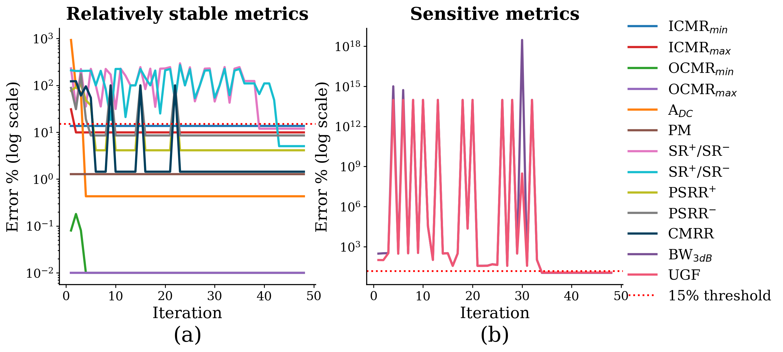
We examine the evolution of the generated equations under the repair loop by tracking their relative error. Figure 4 shows these error trajectories for OTA-2, while Table III reports the convergence iteration and final SPICE-relative error for all five OTAs. As shown in the figure, the repair loop reduces error across successive iterations, although the trajectories are not strictly monotone, since a bounded revision that improves one part of an equation can perturb other coupled terms before later iterations restore accuracy. Sensitive metrics like $BW_{3dB}$ and UGF show larger cross-iteration variation (Figure 4(b)) than the relatively stable metrics (Figure 4(a)). This aligns with their stronger dependence on pole locations and parasitic capacitances, whereas metrics governed by fewer parameters exhibit smoother repair trajectories.

Table III shows that convergence is eventually reached for all five OTAs, with average final relative error below $7\%$ in every case. The required number of repair iterations, however, varies substantially. Considering first the initial testcases before NEMESIS has prior OTA models that can be used for RAG, OTA-1 converges with the least repair effort, consistent with its simple topology, while OTA-2 and OTA-3 require more iterations, indicating greater difficulty in equation generation. For example, OTA-3 is a two-stage OTA that extends the OTA-1 core with an additional common-source stage and therefore serves as a useful intermediate-complexity case; together, OTA-1 through OTA-3 provide a baseline for repair behavior without retrieval. Retrieval is then assessed in OTA-4 and OTA-5, which are initialized using verified equations retrieved from the equation memory. Despite being harder topologies, both converge in fewer repair iterations than OTA-2 and OTA-3, consistent with retrieval providing a stronger initialization and reducing repair effort.

TABLE III: Number of iterations to convergence (Iter.) and final relative error (Err.) (%) for each metric across OTA topologies.

Metric	easycOTA-1		mediumcOTA-2		mediumcOTA-3		hardcOTA-4		hardcOTA-5
	Iter.	% Err.	Iter.	% Err.	Iter.	% Err.	Iter.	% Err.	Iter.	% Err.
ADC	2	2.57%	4	0.43%	3	0.54%	4	6.80%	1	5.87%
PM	8	0.17%	3	1.27%	3	8.91%	15	0.51%	6	2.31%
SR+	12	10.86%	43	11.91%	4	10.91%	14	11.03%	16	11.88%
SR-	11	10.54%	39	8.28%	1	4.14%	3	9.08%	14	9.45%
CMRR	2	9.61%	2	1.44%	13	1.54%	10	6.83%	17	14.22%
PSRR+	7	9.44%	6	4.12%	4	2.52%	10	6.53%	25	4.09%
PSRR-	9	4.37%	5	8.53%	28	10.57%	4	0.59%	1	9.72%
ICMRmin	8	5.63%	43	13.66%	43	0.03%	15	13.64%	12	9.77%
ICMRmax	1	13.68%	2	9.92%	1	5.06%	2	9.81%	2	11.72%
OCMRmin	3	5.05%	1	1.59%	3	0.02%	12	0.81%	4	0.23%
OCMRmax	2	3.15%	4	4.75%	1	0.03%	2	0.17%	1	0.81%
BW3dB	12	4.43%	34	5.97%	44	6.51%	18	0.71%	14	1.59%
UGF	12	5.52%	34	5.98%	39	7.49%	11	4.74%	12	5.99%
Max Iter. / Avg. Err. (%)	12	6.54%	43	5.98%	44	4.28%	18	5.48%	25	6.74%

III-C Accuracy across application-specific $g_{m}/I_{D}$ range

Next, we evaluate whether the converged equations remain accurate over the assigned $g_{m}/I_{D}$ bias range of each OTA, which spans the intended bias space of the topology from higher-speed through balanced to higher-efficiency operation. Starting from the equations that converge at the selected $g_{m}/I_{D}$ value, we realize the nominal point together with additional representative points spanning the full primitive-level $g_{m}/I_{D}$ ranges, including boundary and interior cases, using the LUT-based sizing flow of Section II-C. The equations are then reevaluated at each realized operating point using updated .op-extracted parameters. In the evaluated testcases, no additional repair was required within the assigned ranges, since the equations that converged at the selected $g_{m}/I_{D}$ value remained accurate throughout the evaluated bias space.

Figure 5 shows representative OTA-2 metrics, for which the equation-based predictions remain close to SPICE across the evaluated $g_{m}/I_{D}$ range. The full results for all OTAs are summarized in Table IV. Across the evaluated $g_{m}/I_{D}$ ranges, the average mean relative error remains below $7\%$ for all five OTAs, with many metrics showing substantially lower error. Overall, the converged equations remain usable across the application-specific $g_{m}/I_{D}$ ranges.

TABLE IV: Mean ($\mu$) and standard deviation ($\sigma$) of % error of the equations across the application-specific $g_{m}/I_{D}$ range.

Metric	easycOTA-1		mediumcOTA-2		mediumcOTA-3		hardcOTA-4		hardcOTA-5
	$\mu$	$\sigma$	$\mu$	$\sigma$	$\mu$	$\sigma$	$\mu$	$\sigma$	$\mu$	$\sigma$
ADC	1.15	0.08	0.54	0.34	0.52	0.05	2.51	1.45	1.89	0.76
PM	0.04	0.02	1.01	0.22	9.93	0.95	3.55	0.84	2.41	1.44
SR+	4.64	3.49	9.89	5.21	13.66	2.43	7.89	4.11	11.12	2.69
SR-	9.04	1.97	9.65	4.39	3.24	0.78	8.88	2.69	9.8	1.01
CMRR	3.61	3.88	3.89	1.30	1.73	1.53	2.73	0.58	3.17	0.95
PSRR+	4.14	1.00	1.86	1.98	1.19	0.39	3.41	1.66	5.2	2.04
PSRR-	1.92	0.59	4.07	2.00	7.75	1.24	3.55	2.03	4.59	3.61
ICMRmin	3.67	4.48	9.97	5.09	9.04	2.31	7.54	6.12	5.17	4.68
ICMRmax	0.32	1.42	3.36	1.67	5.69	0.86	1.58	0.81	2.66	3.22
OCMRmin	10.90	3.07	7.65	1.77	4.56	1.98	5.10	0.47	4.59	2.41
OCMRmax	1.92	6.59	3.14	4.27	3.15	1.10	1.08	0.39	1.77	0.98
BW3dB	3.57	1.27	4.86	3.59	8.44	0.50	9.84	2.91	8.19	4.36
UGF	3.85	0.30	4.98	1.58	12.73	2.74	11.79	4.51	5.88	6.59

Figure 5: Accuracy of the converged equations for OTA-2 across representative $g_{m}/I_{D}$ sweep points spanning different inversion regions.

TABLE V: Runtime comparison: Full HSPICE versus equation-based evaluation with .op and equation breakdown.

Topology	SPICE-based evaluation	.op evaluation	Equation evaluation	Total	Speedup
OTA-1	6.74s	1.08ms	0.22ms	1.30ms	5184$\times$
OTA-2	6.89s	1.34ms	0.29ms	1.63ms	4226$\times$
OTA-3	6.99s	1.16ms	0.28ms	1.44ms	4854$\times$
OTA-4	7.05s	1.28ms	0.31ms	1.59ms	4434$\times$
OTA-5	7.11s	1.31ms	0.30ms	1.61ms	4416$\times$

Figure 6: Evolution of the OTA-2 DC-gain equation across repair iterations 1 to 4. Red circles indicate the relative error at each iteration.

Netlist only

Netlist + schematic image

Figure 7: Primitive-device mappings predicted by the LLM for OTA-2 under netlist-only and netlist + schematic-image inputs.

III-D NEMESIS vs. SPICE-based evaluation runtime

We compare post-convergence evaluation in NEMESIS against the full HSPICE verification flow, excluding the one-time model-construction stage. In the SPICE baseline, all target metrics are obtained from the metric-specific testbenches described in Section II-D. After convergence, NEMESIS estimates the same metrics using one .op extraction, which takes only a few milliseconds, followed by direct evaluation of the converged equations.

As detailed in Table V, the NEMESIS-generated OTA model yields a 4226$\times$–5184$\times$ speedup over the complete SPICE testbench flow by computing all metrics at a single realized operating point rather than repeating full DC/AC/TRAN sweeps. During the excluded model-construction stage, each LLM call typically took 30sec–2min, which is dominated by API latency and server traffic.

III-E Interpretability through equation evolution

In addition to improving accuracy, the NEMESIS repair loop preserves interpretability by expressing each repair in device-level small-signal terms. Figure 6 shows this behavior for the DC-gain equation of OTA-2 over four repair iterations. In this example, Iteration 1 is an initial LLM-generated equation lacking reliable circuit interpretation, reflecting the incompleteness or hallucinated term selection typical of a first-pass symbolic guess before SPICE-grounded repair.

From Iteration 2 onward, the equation connects directly to the circuit structure. For example, the $g_{ds_{M7}}+g_{ds_{M9}}$ term is physically meaningful because M7 and M9 connect to the output node, contributing to the small-signal conductance seen at $v_{out}$. Later iterations introduce additional conductance terms, clarifying that gain is affected by the conductances associated with the output node and internal nodes in the bias and mirror network. The inclusion of $g_{m_{M4}}$ and $g_{m_{M6}}$ in the final iteration is also circuit-consistent, as M4 and M6 are diode-connected PMOS devices whose small-signal transconductance contributes to the conductance at the corresponding internal nodes. Ultimately, interpretability stems from the repaired equation itself: as the expression is corrected, it becomes both more accurate with respect to SPICE and more useful for manual analysis, with terms remaining traceable to specific devices and node loading in the topology.

III-F Ablation and sensitivity studies

We present three studies to assess key components of NEMESIS: multimodal circuit input, equation memory retrieval, and the convergence threshold $\epsilon$ in the repair loop.

Ablation on multimodal input: Figure 7 compares primitive extraction for OTA-2 using netlist-only and netlist-plus-schematic inputs. With netlist-only input, the LLM omits M6 from the active-load group, misassigns M8 to the bias current mirror, and introduces a nonexistent second_stage block. Adding the schematic image corrects these errors and aligns the primitive groups with the intended topology. Similar netlist-only errors were observed across all OTAs, indicating that multimodal input improves structural grounding and reduces topology hallucinations during primitive extraction.

Ablation on equation memory retrieval: To isolate the effect of retrieval, we repeated OTA-4 and OTA-5 without equation memory. The repair iterations increased from 18 to 61 for OTA-4 and from 25 to 57 for OTA-5. Retrieval primarily improves initialization and reduces repair effort.

TABLE VI: Number of iterations (Iter.) and percentage error (Err.) w.r.t. SPICE for OTA-1 for each metric, for $\epsilon=15\%$ and $\epsilon=5\%$.

Metric	Iter. @15%	Err. @15%	Iter. @5%	Err. @5%
ADC	2	2.57%	5	1.22%
PM	8	0.17%	17	0.02%
SR+	12	10.86%	16	4.37%
SR-	11	10.54%	12	4.66%
CMRR	2	9.61%	10	1.53%
PSRR+	7	9.44%	20	4.71%
PSRR-	9	4.37%	11	2.23%
ICMRmin	8	5.63%	10	3.51%
ICMRmax	1	13.68%	3	0.44%
OCMRmin	3	5.05%	5	4.58%
OCMRmax	2	3.15%	3	1.88%
BW3dB	12	4.43%	17	2.69%
UGF	12	5.52%	14	3.49%
Max Iter. / Average Err.	12	6.54%	20	2.67%

Sensitivity to convergence threshold: We repeat the repair loop for all five OTAs after tightening the error threshold from $15\%$ to $5\%$. The stricter threshold reduces the final average error to below $5\%$ for every topology, while keeping the maximum repair effort below 45 iterations. Table VI shows detailed per-metric OTA-1 results as a representative case, where average final relative error decreases from $6.54\%$ to $2.67\%$. This illustrates the expected tradeoff between stricter accuracy targets and increased repair effort.

IV Conclusion

This paper presented NEMESIS, a multimodal LLM framework for generating OTA performance equations from SPICE netlists and schematics using SPICE-based verification and iterative repair. Across five OTA topologies, NEMESIS produced interpretable device-level equations whose predictions closely align with SPICE over assigned $g_{m}/I_{D}$ ranges. By providing physical circuit insight without manual derivation, NEMESIS enables fast equation-based evaluation for repeated design exploration. However, (a) it assumes that the topology is fixed; (b) it does not replace final SPICE signoff. Extensions to large-signal nonlinearities, phase noise, high-frequency matching, and modeling for variable topologies in topology optimization are topics for future work.

References

- [1] (2022) A hierarchical performance equation library for basic op-amp design. IEEE Transactions on Computer-Aided Design of Integrated Circuits and Systems 41 (7), pp. 1976–1989. Cited by: §I, §I.
- [2] (2026) ALIGN: Analog Layout, Intelligently Generated from Netlists. Note: https://github.com/ALIGN-analoglayout/ALIGN-public/tree/master/CircuitsDatabase/Generalized_Testbenchesaccessed on Jan. 21, 2026 Cited by: §II-D.
- [3] (2021) DNN-Opt: An RL inspired optimization for analog circuit sizing using deep neural networks. In Proceedings of the ACM/IEEE Design Automation Conference, Vol. , pp. 1219–1224. Cited by: §I.
- [4] (2022) An efficient analog circuit sizing method based on machine learning assisted global optimization. IEEE Transactions on Computer-Aided Design of Integrated Circuits and Systems 41 (5), pp. 1209–1221. Cited by: §I.
- [5] (2024) Artisan: Automated operational amplifier design via domain-specific large language model. In Proceedings of the ACM/IEEE Design Automation Conference, Note: 6 pages Cited by: §I, §I.
- [6] (2023) MA-Opt: Reinforcement learning-based analog circuit optimization using multi-actors. In Proceedings of the Design, Automation & Test in Europe Conference, Note: 5 pages Cited by: §I.
- [7] (2003) Simulation-based generation of posynomial performance models for the sizing of analog integrated circuits. IEEE Transactions on Computer-Aided Design of Integrated Circuits and Systems 22 (5), pp. 517–534. Cited by: §I.
- [8] (1998) GPCAD: A tool for CMOS op-amp synthesis. In Proceedings of the IEEE/ACM International Conference on Computer-Aided Design, pp. 296–303. Cited by: §I.
- [9] (2026) Parasitics-aware framework for integrated OTA sizing and layout synthesis in FinFET technologies. In Proceedings of the IEEE International Symposium on Quality Electronic Design, Note: 9 pages Cited by: §I.
- [10] (2025) Accelerating OTA circuit design: transistor sizing based on a transformer model and precomputed lookup tables. In Proceedings of the Design, Automation & Test in Europe Conference, Vol. . Note: 7 pages Cited by: §I.
- [11] (1990-06) Analog circuit design optimization based on symbolic simulation and simulated annealing. IEEE Journal of Solid-State Circuits 25 (3), pp. 707–713. Cited by: §I.
- [12] (2001) The sizing rules method for analog integrated circuit design. In Proceedings of the IEEE/ACM International Conference on Computer-Aided Design, Vol. , pp. 343–349. Cited by: §I, §I.
- [13] (2024) tSS-BO: Scalable Bayesian optimization for analog circuit sizing via truncated subspace sampling. In Proceedings of the Design, Automation & Test in Europe Conference, Vol. . Note: 6 pages Cited by: §I.
- [14] (1989-12) OASYS: A framework for analog circuit synthesis. IEEE Transactions on Computer-Aided Design of Integrated Circuits and Systems 8 (12), pp. 1247–1266. Cited by: §I.
- [15] (1901) Étude comparative de la distribution florale dans une portion des alpes et des jura. Bulletin de la Société Vaudoise des Sciences Naturelles 37, pp. 547–579. Cited by: §II-A.
- [16] (2017) Systematic design of analog CMOS circuits: using pre-computed lookup tables. Cambridge University Press, Cambridge, UK. External Links: ISBN 9781108136730 Cited by: 3rd item, §I, §II-C.
- [17] (2025) LEDRO: LLM-enhanced design space reduction and optimization for analog circuits. In Proceedings of the IEEE International Conference on LLM-Aided Design, Vol. , pp. 141–148. Cited by: §I, §I.
- [18] (1990) OPASYN: A compiler for CMOS operational amplifiers. IEEE Transactions on Computer-Aided Design of Integrated Circuits and Systems 9 (2), pp. 113–125. Cited by: §I.
- [19] (2020) GANA: Graph convolutional network based automated netlist annotation for analog circuits. In Proceedings of the Design, Automation & Test in Europe Conference, Vol. , pp. 55–60. Cited by: §I.
- [20] (2019) ALIGN: Open-source analog layout automation from the ground up. In Proceedings of the ACM/IEEE Design Automation Conference, Note: 4 pages Cited by: §II-D.
- [21] (2025) AnalogCoder: Analog circuit design via training-free code generation. In Proceedings of the AAAI Conference on Artificial Intelligence, Note: 9 pages Cited by: §I, §I.
- [22] (2020) Retrieval-augmented generation for knowledge-intensive NLP tasks. In Advances in Neural Information Processing Systems, Note: 16 pages Cited by: §I.
- [23] (2025) EEschematic: Multimodal-LLM based AI agent for schematic generation of analog circuit. arXiv preprint arXiv:2510.17002. Note: 5 pages Cited by: §II-B.
- [24] (2024) AmpAgent: An LLM-based multi-agent system for multi-stage amplifier schematic design from literature for process and performance porting. arXiv preprint arXiv:2409.14739. Note: 7 pages Cited by: §I, §I.
- [25] (2018-06) An efficient Bayesian optimization approach for automated optimization of analog circuits. IEEE Transactions on Circuits and Systems I 65 (6), pp. 1954–1967. Cited by: §I.
- [26] (2018) Batch Bayesian optimization via multi-objective acquisition ensemble for automated analog circuit design. In Proceedings of the International Conference on Machine Learning, pp. 3306–3314. Cited by: §I.
- [27] (2001) CMOS op-amp sizing using a geometric programming formulation. IEEE Transactions on Computer-Aided Design of Integrated Circuits and Systems 20 (1), pp. 22–38. Cited by: §I.
- [28] (2008) The sizing rules method for CMOS and bipolar analog integrated circuit synthesis. IEEE Transactions on Computer-Aided Design of Integrated Circuits and Systems 27 (12), pp. 2209–2222. Cited by: §I.
- [29] (2025) GPT-5.2 model. Note: https://developers.openai.com/api/docs/models/gpt-5.2accessed on Jan. 23, 2026 Cited by: §I, §III-A.
- [30] (2025) GENIE-ASI: Generative instruction and executable code for analog subcircuit identification. arXiv preprint arXiv:2508.19393. Note: 21 pages Cited by: §I.
- [31] (2020) AutoCkt: Deep reinforcement learning of analog circuit designs. In Proceedings of the Design, Automation & Test in Europe Conference, Note: 6 pages Cited by: §I.
- [32] (2026) Atelier: An automated analog circuit design framework via multiple large language model-based agents. IEEE Transactions on Computer-Aided Design of Integrated Circuits and Systems 45 (1), pp. 31–44. Cited by: §I, §I.
- [33] (2011-11) Weisfeiler-Lehman graph kernels. Journal of Machine Learning Research 12, pp. 2539–2561. Cited by: §II-A.
- [34] (1996-10) A / based methodology for the design of CMOS analog circuits and its application to the synthesis of a silicon-on-insulator micropower OTA. IEEE Journal of Solid-State Circuits 31 (9), pp. 1314 – 1319. External Links: Document Cited by: §I.
- [35] (2021) Local Bayesian optimization for analog circuit sizing. In Proceedings of the ACM/IEEE Design Automation Conference, pp. 1237–1242. Cited by: §I.
- [36] (2020) GCN-RL circuit designer: Transferable transistor sizing with graph neural networks and reinforcement learning. In Proceedings of the ACM/IEEE Design Automation Conference, Note: 6 pages Cited by: §I.
- [37] (2024) ADO-LLM: Analog design Bayesian optimization with in-context learning of large language models. In Proceedings of the IEEE/ACM International Conference on Computer-Aided Design, Note: 9 pages Cited by: §I, §I.