

Near-real-time, meter-scale 3D urban wind modeling for low-altitude micrometeorology: numerical verification of a GPU-accelerated lattice Boltzmann framework
Abstract
This study presents a near-real-time, meter-scale three-dimensional urban wind simulation framework for low-altitude flight events in complex urban meteorological environments. It reconstructs high-resolution wind fields by combining sparse observations with efficient microscale flow modeling. The framework integrates lattice Boltzmann method large-eddy simulation (LBM-LES), high-fidelity urban morphology reconstruction that explicitly resolves real building details, and observation-driven boundary assimilation into a rapid end-to-end pipeline for realistic urban domains. Multi-site Doppler lidar measurements from dense urban Guangzhou, China, are used for evaluation. The system reconstructs three-dimensional wind fields at 5 m resolution over kilometer-scale domains within minutes. Robustness and accuracy are tested through controlled observation reduction, independent validation against withheld lidar stations, and sensitivity analyses of grid resolution and precursor domain extent. Results show stable reproduction of vertical wind structures and key local flow features under complex morphology and limited observations, providing a scalable pathway for near-real-time urban wind reconstruction.
keywords:
High-fidelity urban wind simulation , computational fluid dynamics , lattice Boltzmann method , model verification[label1] organization=National Meteorological Information Centre, addressline=China Meteorological Administration, city=Beijing, postcode=100081, country=China
[label2] organization=Department of Civil and Environmental Engineering, addressline=University of California Berkeley, city=Berkeley, postcode=94704, state=CA, country=United States
[label3] organization=Department of Mechanical and Aerospace Engineering, addressline=The University of Manchester, city=Manchester, postcode=M13 9PL, country=UK
[label5] organization=Department of Building Environment, addressline=National University of Singapore, postcode=119077, country=Singapore
[label4] organization=College of Automotive and Energy Engineering, addressline=Tongji University, city=Shanghai, postcode=201804, country=China
[label6] organization=Beijing Fengyun Meteorological Science and Technology Development Co., Ltd., city=Beijing, postcode=100081, country=China
[label7] organization=School of Artificial Intelligence, addressline=Sun Yat-sen University,city=Zhuhai, postcode=519000, state=Guangdong Province, country=China
[label8] organization=Ralph O’Connor Sustainable Energy Institute, addressline=Johns Hopkins University, city=Baltimore, postcode=21218, state=MD, country=United States
[label9] organization=Beijing Aeronautical Science and Technology Research Institute, addressline=The Commercial Aircraft Corporation of China, city=Beijing, postcode=102211, country=China \affiliation[label10] organization=The Key Laboratory of Road and Traffic Engineering of Ministry of Education, Tongji University, city=Shanghai, postcode=201804, country=China
1 Introduction
The rapid rise of the low-altitude economy and urban air mobility (UAM) is reshaping how cities move people and deliver services [11, 3, 24]. Low-altitude operations such as drone logistics, urban air mobility, emergency response, inspection, and surveying typically fly close to the ground surface, demand strong timeliness, and unfold in highly complex environments [52, 46, 11]. As a result, meteorological conditions have evolved from an important constraint in conventional aviation support into a primary basis for developing and exploiting the spatiotemporal resources of low-altitude airspace [53, 46]. In particular, the three-dimensional wind field and its rapid variability affect vehicle stability, control margins, trajectory tracking, energy consumption, and mission success. They also define safe operating envelopes over complex urban surfaces [52, 46]. In megacities, the combined effects of building clusters, street canyons, green space, and water bodies modify near surface momentum and heat exchange, generating strong spatial heterogeneity and multiscale coupling [14, 32, 31, 7]. Street-canyon geometry has long been recognized as a primary control on canyon-scale flow channeling and ventilation pathways [43]. Reviews of street-canyon flow and dispersion further document recirculation zones, flow separation, and downstream reattachment generated by urban canyon vortices [58]. At the building and district scales, computational wind engineering studies report local wind acceleration near corners and roof edges together with separated wakes around bluff bodies [5], while the AIJ practical CFD guidelines identify separation and reattachment around buildings as core validation targets for urban flow simulations [57]. Recent evaluation of a multilayer urban canopy model across contrasting urban contexts likewise confirms that representing urban morphological effects remains essential for reproducing these microscale wind responses [51]. Aircraft participating in the low-altitude economy and UAM often operate within the low-altitude airspace of 0–1000 m [66, 65, 55], which coincides with the region characterized by these strong turbulence and unsteady flow phenomenon [13], further underscoring the importance of acquiring small-scale flow information for general aviation [63]. High-quality three-dimensional wind simulation and refined wind field analysis have consequently become central challenges for urban meteorological support and the development of low-altitude meteorological service capability [6, 48].
Operational monitoring and warning for strong winds rely mainly on observation systems such as Doppler lidar wind profilers, meteorological towers, and automatic weather stations [38]. Mature services have been established in high impact sectors including coastal ports, urban rail transit, and construction sites [11, 38]. These systems provide reliable time series observations that support the identification of regional strong wind events and the issuance of warnings [59]. However, conventional wind observing systems face intrinsic limits in representativeness [38]. On the one hand, sensitivity, saturation effects, and instrument inertia can introduce dynamic errors when measuring intense gusts or rapidly changing flow [36]. On the other hand, point-based observations struggle to capture the sharp spatial contrasts of small-scale urban winds [14]. Given constraints on space, staffing, maintenance, and equipment cost, engineering a dense enough network to reconstruct accurate three-dimensional winds over a small urban area is not realistic [38]. The resulting service granularity remains insufficient for low-altitude flight [52, 46]. For example, when strong winds approach, current products often cannot provide actionable quantitative guidance on the differing small-scale risks across specific corridors or route segments, which limits professional and fine-grained low-altitude meteorological support [52, 46].
Numerical weather prediction models improve service coverage through gridded forecasts and are a key pathway to continuous depiction of regional wind fields [2, 44]. The forecast quality of fine scale wind structures depends strongly on how well processes such as deep convection, boundary layer turbulence, and interactions with urban surfaces are represented [48, 32, 31]. Many studies have shown that increasing horizontal resolution helps resolve the physical processes and detailed structures of small-scale weather systems [47, 50, 45]. Yet convective storms are highly localized, abrupt, and fast evolving, and reliable prediction often requires robust subkilometre high resolution simulation [44, 48]. In recent years, advances in supercomputing and parallelization have pushed mesoscale model resolution toward the kilometre scale, but further refinement to subkilometre and finer scales faces substantial challenges due to limits in dynamical frameworks and vertical coordinate systems [2, 48]. Finer-scale simulations demand higher-fidelity terrain and land-use data and surface parameterizations that represent urban morphology (e.g., building arrays, street canyons, and vegetation) [39]. These elements are required to capture urban impacts on local winds at minute-level temporal resolution and meter-scale spatial resolution [14, 32, 31]. Traditional mesoscale models often struggle to maintain both physical consistency and computational affordability in this regime [2, 48].
For urban microscale problems, computational fluid dynamics (CFD) provides an effective means to represent complex geometric boundaries and local turbulent structures [42], delivering high resolution wind and temperature fields that support risk identification for low-altitude corridors [8], evaluation of takeoff and landing site suitability [61], building and pedestrian ventilation [18], and urban environmental management [4]. With improved hardware performance and higher efficiency in high performance parallel computing, real-time or near-real-time simulation over complex urban districts is becoming increasingly feasible [26, 64]. Nonetheless, key trade-offs remain. Large-eddy simulation (LES) resolves large scale turbulent motions and uses subgrid scale models for smaller scales, typically achieving high turbulence fidelity, but at prohibitive computational cost for large urban domains and operational timeliness requirements [35, 5]. Reynolds averaged Navier-Stokes simulations (RANS) reduce cost through flow averaging and are easier to deploy, but rely on Reynolds stress closure and therefore introduce turbulence model error [5, 57]. Meanwhile, urban roughness and surface parameterizations remain immature, leading to unstable accuracy in complex urban morphologies and limiting their ability to support the fine-grained risk quantification required for low-altitude operations [14, 32, 31, 6].
The lattice Boltzmann method (LBM), which has developed rapidly in recent years, is a mesoscopic computational fluid dynamics approach with relatively simple formulations of fluid interactions, convenient treatment of complex boundaries, high parallel efficiency, and a clear implementation pathway [1, 12]. These features suggest potential advantages for complex geometry and large-scale parallel computation [26, 49]. For the microscale three-dimensional wind field needs of low-altitude operations in cities, the efficiency and boundary handling properties of lattice Boltzmann methods may offer a promising technical option that balances high resolution with operational usability [64, 23]. However, from the perspective of meteorological support for the low-altitude economy, a clear discontinuity remains between existing research and operational systems [6, 52, 64]. Existing urban microscale wind studies have addressed a broad range of built-environment applications, including urban wind-resource evaluation and wind-turbine feasibility [56], morphology-based classification of local ventilation performance zones [28], physics-based assessment of wind damage to building clusters [15], and wind-induced interference effects around high-rise buildings [60]. These studies collectively highlight the importance of resolving urban morphology, local ventilation pathways, and building-scale flow interactions. However, their problem settings are still mainly oriented toward wind-environment assessment, design support, or post-event risk evaluation, rather than observation-constrained, corridor-oriented low-altitude meteorological services. Boundary forcing, the precision of urban morphology data, and standards for systematic validation against observations also remain insufficiently unified, making results difficult to translate into reusable city-scale products [57, 4, 6]. Operational low-altitude meteorological services, by contrast, emphasize minute level updates, metre to hectometre scale spatial guidance, and interpretable risk factor outputs [52, 46]. Yet current observation networks cannot provide sufficiently dense three-dimensional constraints, conventional mesoscale models cannot resolve urban morphological detail, and classical microscale methods have not resolved the core tension between cost and accuracy [38, 48, 5, 35]. Zhang et al. [64] developed TH-MuSiC, a high-efficiency WRF-LBM platform. However, the end-to-end workflow still requires tens of minutes for domains with tens of millions of cells. Overall, a key research gap persists: a technical route that can stably produce high resolution three-dimensional wind fields over complex urban surfaces at an affordable computational cost, while synergizing with existing meteorological observation and forecasting systems [2, 6]. Moreover, the numerical methods [20], mesh strategy [19] and domain configurations are also worth noting to ensure the reliability.
In this study, we develop and verify a near-real-time, meter-scale three-dimensional urban wind reconstruction framework aimed at providing operational meteorological support for low-altitude applications over complex city environments. The framework integrates high-fidelity urban morphology reconstruction with a GPU-accelerated LBM-LES solver powered by FluidX3D. Sparse multi-site Doppler lidar measurements are used to build observation-driven boundary conditions via gridded volumetric wind reconstruction and conservative boundary correction, forming an end-to-end pipeline that can deliver kilometer-scale 3D wind fields within minutes. Using a dense lidar deployment over Haixinsha Island and its surroundings in Guangzhou, we conduct numerical verifications via independent station holdout and progressive reductions of observational inputs to assess robustness under limited constraints, and further examine the sensitivity of reconstructed winds to lattice resolution and precursor-domain extent to clarify the dominant numerical factors governing accuracy and stability.
The remainder of this paper is organized as follows. Section 2 describes the integrated preprocessing, boundary reconstruction, and the GPU LBM-LES implementation. Section 3 introduces the study area, lidar observations, and experimental design. Section 4 presents validation results and sensitivity analyses. Section 5 summarizes the main findings and discusses implications for near-real-time low-altitude meteorological services.
2 Numerical methods
We developed a comprehensive simulation pipeline that integrates geospatial preprocessing, conservative boundary reconstruction, voxel-based geometry handling, and FluidX3D, the GPU-accelerated LBM kernel. The solver incorporates LES closure and Coriolis forcing to accurately capture atmospheric flow dynamics.
2.1 Geospatial preprocessing and boundary reconstruction
To ensure geometric fidelity, all geospatial inputs are first transformed into a metric projected coordinate system suitable for uniform Cartesian grids. Because map projection can distort rectangular longitude-latitude extents, the computational domain is re-clipped in the projected space to recover an axis-aligned rectangular region compatible with structured meshing. Terrain elevations derived from the Digital Elevation Model (DEM) are interpolated from scattered samples to a regular raster using Inverse Distance Weighting (IDW), followed by smoothing with a discrete Gaussian kernel. This process suppresses small-scale noise while retaining large-scale topographic gradients. During subsequent processing, terrain height values are retrieved via fast bilinear interpolation on this precomputed raster. Details of the terrain-layer construction are provided in B.
Building placement is rendered terrain-consistent by aligning the building base to the local minimum terrain elevation over its footprint, thereby avoiding gaps or solid overlaps at the ground interface. Both buildings and terrain are mapped onto the Cartesian lattice through voxelization. A ray-tracing-based occupancy test efficiently classifies solid and fluid cells over large-scale domains. The final solid mask is assembled by the Boolean merging of a fixed-thickness base layer, the terrain layer, and the building layer, yielding a unified no-slip boundary representation. Since Cartesian voxelization introduces a staircase approximation, spatial resolution is treated as a governing modeling parameter for geometric fidelity and near-wall momentum exchange.
Boundary wind conditions are derived via a two-stage downscaling strategy designed to balance accuracy and throughput. First, the irregular point field in projected space is interpolated to an intermediate Cartesian grid using Delaunay triangulation, employing barycentric coordinates for linear interpolation to preserve local gradients without extraneous smoothing. For targets outside the triangulation convex hull, the procedure reverts to a nearest-neighbor assignment accelerated by a k-dimensional (k-d) tree. Second, the intermediate boundary field is mapped onto the CFD boundary nodes. This step utilizes either a nearest scheme for maximum computational speed or an improved k-Nearest Neighbor (kNN) reconstruction for smoother, more stable fields. The improved method employs a fixed neighborhood size, inverse distance squared weighting, and an adaptive stabilization term to prevent numerical sensitivity at minimal distances, while applying a consistent weight set across all velocity components to maintain vector coherence. The full two-stage velocity-interpolation procedure is shown in C.
To mitigate spurious compressibility and net volume imbalance inherent in imperfect atmospheric boundary data, we apply a mass flux consistency correction at each boundary. This correction eliminates mean normal flux bias by applying the minimal normal velocity adjustment required to enforce near-zero net volume flow, ensuring the interpolated boundary field remains as close to the original data as possible.
2.2 Lattice Boltzmann flow solver and implementation
The refined urban wind simulation employs the mesoscopic LBM based on FluidX3D. Compared to traditional CFD solvers based on macroscopic continuum mechanics, LBM offers distinct advantages, including algorithmic simplicity, minimal numerical dissipation, and inherent capability in handling complex boundaries. The method utilizes an explicit time-integration scheme where the non-linear collision term is local and the linear streaming step requires no interpolation. These characteristics eliminate the need for global matrix inversions and guarantee high computational efficiency and ease of parallelization. In the LBM framework, the continuous phase space is discretized by a finite set of virtual particle velocities. This discrete velocity scheme serves two critical functions: it reduces the infinite motion modes of real fluid molecules to a computable finite set, and it discretizes continuous space by defining the distance virtual particles travel per time step. This approach replaces the physical mesh and finite-difference discretizations used in traditional CFD, thereby reducing errors associated with mesh generation and discretization schemes.
In this study, we adopt the D3Q19 discrete velocity model, where denotes the spatial dimension and represents the number of discrete velocity directions. The D3Q19 model is widely validated for simulating three-dimensional flows across various urban scales, ranging from isolated buildings to complex street canyons and city blocks. The flow field evolution is governed by the Single Relaxation Time (SRT) collision operator on a uniform lattice. Subgrid-scale stresses are modeled using the Smagorinsky-Lilly model within an LES framework. Open boundaries are managed via equilibrium-based velocity constraints and reflection suppression to minimize artificial wave return, while ground, terrain, and buildings are imposed as no-slip walls. A dimensionless scaling scheme adaptively matches the reference wind speed to a target LBM Mach number, ensuring numerical stability under high winds. Earth rotation effects are incorporated through a Coriolis body force evaluated directly within the GPU kernel. The rotation vector is expressed in the local East-North-Up (ENU) frame at the domain latitude, consistently converted into lattice units, and integrated using a Guo-type forcing discretization. A complete description of the LBM formulation and the FluidX3D-based implementation is provided in D, and the Coriolis forcing term is detailed in E.
The implementation follows a hybrid CPU-GPU architecture. The CPU handles preprocessing, constructing and caching interpolation search structures such as triangulations and k-d trees with full parallel-computing capability. Meanwhile, GPU kernels execute the computationally intensive per-step macroscopic reconstruction, source term assembly, and lattice updates. This organization minimizes synchronization overhead and data movement, enabling efficient simulation over extremely large structured grids.
3 Investigated region and observations
Geographically, the study area is situated between longitudes E and E, and latitudes N and N, encompassing Haixinsha Island and its vicinity in Guangzhou, Guangdong Province of China. The x-axis and y-axis are first established in the east and north directions, respectively, followed by a correction rotation determined by the calculated meridian convergence angle of . The simulation domain extends approximately m along the x-axis and m along the y-axis. The building database used in this case is taken from the 3D-GloBFP dataset [9], and the DEM databases are taken from the NASADEM global digital elevation model [40]. The buildings in the computational region are shown in Figure 1. The model employs a uniform horizontal and vertical grid resolution of 5 m, which is later shown to be the coarsest tested resolution that still preserves the essential building geometry and near-ground profile structure in the present urban setting, while remaining computationally practical.

| No. | Station ID | Time resolution | Vertical resolution (m) | Start height (m) | Max height (m) |
| 1 | GAW102 | 1 min | 13 | 43 | 442 |
| 2 | GAW103 | 1 min | 13 | 52 | 2455 |
| 3 | GAW104 | 1 min | 13 | 52 | 2455 |
| 4 | GAW105 | 10 min | 14 | 85 | 2828 |
| 5 | GAW110 | 1 min | 53 | 42 | 1058 |
| 6 | GAW111 | 1 min | 13 | 52 | 2455 |
Six Doppler light detection and ranging (lidar) systems were deployed within this region, with the station IDs listed in Table 1 and shown in Figure 2. They are placed on open areas like lawns or parking lots to minimize the impact of surrounding buildings as much as possible. These observations are employed both for boundary construction and for validation. However, within any case, they do not simultaneously serve both roles.

At each analysis time, each lidar site provides quality-controlled horizontal wind components at discrete heights. In the present study, only these horizontal components are assimilated in the boundary reconstruction. This is primarily a methodological choice constrained by the common operational lidar product available consistently across the six sites, rather than an assumption that vertical motions are dynamically negligible. Once initialized, the LBM–LES solver still advances the full three-dimensional velocity field inside the CFD domain; therefore, the restriction applies only to the lidar-based boundary forcing and the direct observation-based validation. Vertical velocity can nevertheless be important in urban flows because building-induced shear layers, rooftop updrafts and downdrafts, wake recirculation, and thermally driven canopy exchange all involve non-negligible vertical transport [5]. In the present operational dataset, however, quality-controlled horizontal winds were the only components available with sufficient cross-site consistency for robust multi-site assimilation. The boundary is constructed using transient observation data (instantaneous wind speeds), supporting a quasi-steady time stepping strategy. After temporal collocation across sites and filtering by quality-control flags, the irregularly distributed samples of the horizontal wind components are modeled as realizations of a spatially correlated random field and reconstructed onto a regular grid. Specifically, for each target height level, a spherical semivariogram is established in the horizontal plane and Ordinary Kriging weights are solved to obtain the minimum-variance linear estimate under the unbiasedness constraint on a regular longitude–latitude grid. The resulting gridded fields at individual height levels are then stacked to form a three-dimensional wind field at the target time. Kriging variance can be evaluated as a by-product to characterize interpolation uncertainty; however, the present analysis focuses on the reconstructed wind components. The use of multiple lidar sites increases spatial sampling and reduces extrapolation near the domain boundaries, thereby improving the robustness and spatial continuity of the reconstructed wind field. See A for algorithm, parameters and other implement details for reproducibility. The reconstructed wind field is then sampled on the domain boundaries to drive the LBM solver. Unless otherwise specified, we reconstruct low-altitude three-dimensional winds within the urban canopy at a spatial resolution of 5 m.
The experimental design employs a strategy of progressive data reduction by systematically decreasing the number of input lidars to validate the accuracy of low-altitude three-dimensional wind fields simulated by the LBM. Consequently, this study assesses the feasibility of reconstructing comprehensive wind fields without observational blind zones using limited and isolated data. To evaluate the simulation capabilities of the LBM model within complex urban environments, four sets of comparative experiments were established. Case 1 utilizes observations from five lidars as boundary condition inputs and reserves one for validation. The subsequent groups systematically reduce the input sources, where Cases 2, 3, and 4 employ four, three, and two lidars for input while reserving two, three, and four stations for validation, respectively. The detailed station IDs used for input and evaluation purposes are listed in Table 2. Candidate periods were screened according to four practical criteria: absence of precipitation, high cross-site data integrity and temporal continuity across the deployed lidar network, moderate-to-strong background winds that provide a stringent verification condition for the CFD model, and relatively stable large-scale forcing without abrupt wind-direction transitions. Because buoyancy effects are not included in the present model configuration, periods dominated by strong thermal-convective signatures were not prioritized, but advection dominated. Under these criteria, the two-hour window from 17:00 to 19:00 (UTC+08:00) on 10 September 2025 provided the best combination of data quality and suitability for independent holdout validation. After quality assurance, the specific validation instants retained for profile comparison, namely 17:10, 18:10, and 18:30, reached maximum valid observation heights of 800 m, 400 m, and 400 m, respectively. The selected case lies within the moderate-to-high wind range of the observed distribution rather than at either the calm or extreme tail, indicating that it is representative of operationally relevant windy conditions while remaining suitable for robust model verification. In addition, smooth cascading energy in wavenumber presented by G further shows that no strong cyclonic flow patterns or large-scale extreme weather events were observed during the monitoring period. It is noteworthy that while the raw lidar observations offer high temporal resolution ranging from minute-level to second-level frequencies, a sampling interval of 10 minutes was adopted for this simulation. This resolution was chosen to achieve an optimal balance between computational efficiency and the temporal representativeness of the data.
| Testing case | Model input stations | Evaluation stations |
| Case 1 | GAW102, GAW103, GAW104, GAW105, GAW110 | GAW111 |
| Case 2 | GAW102, GAW103, GAW104, GAW105 | GAW110, GAW111 |
| Case 3 | GAW102, GAW103, GAW104 | GAW105, GAW110, GAW111 |
| Case 4 | GAW102, GAW103 | GAW104, GAW105, GAW110, GAW111 |
The computational domain and boundary conditions are presented in Figure 3. The boundary conditions are configured as follows: The four lateral faces and the planar top face are prescribed as equilibrium-based open velocity boundaries, with the macroscopic boundary states obtained by face-wise mapping of the preprocessed mesoscale wind field onto the computational boundary. To reduce spurious reflection of outgoing disturbances and to improve numerical stability near the outer domain surfaces, the open-boundary treatment is further supplemented by relaxation-based damping regions adjacent to the upper and lateral boundaries, including a top sponge layer and boundary-adjacent buffer nudging toward the target boundary state; in addition, a global flux-balancing correction is applied over the full set of open boundaries. In contrast, the lower boundary, all cells below the local terrain elevation, and the voxelized building-fluid interfaces are treated as stationary no-slip solid boundaries using the standard mid-grid bounce-back scheme. This configuration imposes mesoscale-informed velocity conditions on the outer domain surfaces while representing the ground and urban obstacles as impermeable no-slip walls. In total, 40000 timesteps are calculated in each case, which corresponds to approximately 85 building-scale turnover time to ensure the convergence of low-order quantities including wind speed and turbulent kinetic energy. Further details on our numerical implementation and developed algorithms will be presented in follow-up sequel of this series paper.

The computations were carried out on a GPU node equipped with an NVIDIA A800 80G, using a single GPU, with the complete computational workflow requiring approximately 5 minutes (domain: 4 km, resolution: 5 m, height: 800 m). In addition, for testing purposes, simulations were also performed on a cost-effective desktop GPU setup consisting of customized NVIDIA RTX 2080 Ti 22G GPU 2, resulting in a total runtime of approximately 8 minutes. These wall-clock times correspond specifically to the present baseline configuration. For the explicit LBM solver, the total computational cost scales primarily with the total number of lattice updates, i.e. approximately with , where is determined by the grid-cell count for the chosen domain and depends on the simulated physical duration and the adopted time-step size . In the baseline case reported here, , s, and , corresponding to 400 s of simulated physical time. Within this specific configuration, the reported runtimes demonstrate the computational efficiency of the proposed numerical methodology and platform.
For the baseline case which uses 5 m grid size, key numerical parameters during the computation are listed as follows: The reference velocity in SI unit is 5.3205 m/s, according to an LBM mach number . The time step is 0.01 s. The geometry nondimensionalization factor is 0.20. The lattice count is 116 million. LBM nondimensionalized volume flux before and after correction is and , respectively, with a mean velocity variation on the surface mesh of 1.974 (positive values indicate an outflow). The maximum LBM Reynolds number is , and the LBM kinematic viscosity is . The terrestrial convergence angle at the center of the computational region is based on UTM 49N.
4 Results and discussion
4.1 Convergence of mesh and re-voxelization
Mesh strategy has a significant impact on the numerical results [19, 54]. We re-voxelize the triangle mesh by casting axis-aligned rays through grid columns and computing ray–triangle intersections, using an odd–even parity rule along each column. To improve robustness near degeneracies, we corroborate independent passes along different ray directions for solid labeling.
Due to the adoption of a uniform, isotropic Cartesian grid, the mesh does not conform to the body geometry, which inevitably gives rise to a stair-step approximation effect. Consequently, the resulting solid grid is geometrically inconsistent with the actual building model at the boundaries. Employing a finer spatial discretization enables a more faithful reconstruction of the geometric details of the building, thereby leading to more accurate numerical predictions. Moreover, after orthogonal projection onto the principal axes, buildings whose shorter lateral dimension is smaller than the grid resolution are neglected. As a result, the ground friction effect is underestimated [30]. Although this deficiency can be partially compensated through boundary assimilation effect, particularly from the top boundary, the grid resolution remains the most dominant factor governing the global accuracy. The target grid resolution required in practice is governed by the local distribution of building dimensions as well as the relative weighting between buildings and terrain. Guangzhou is characterized by predominantly flat terrain with minimal elevation variations. Therefore, we primarily focus on the stair-step approximation effects induced by buildings.
The distribution of building sizes within the computational domain is characterized using the probability density function (PDF) and the cumulative distribution function (CDF), obtained by integrating over building volume (Figure 4(a)). It can be observed that the building population in the domain is dominated by small-scale structures: approximately 80% (by volume) of the buildings have a shorter lateral dimension smaller than 50 m, which poses a significant challenge for accurate numerical representation. Five grid resolutions are employed, namely 2 m, 5 m, 10 m, 20 m, and 50 m, as marked in Figure 4(a). The original triangulated representation of the buildings is shown in Figure 4(b). As the velocity inside solid regions is zero, isosurfaces defined by m/s is used to approximate the effective solid-envelope surface, as illustrated in Figure 4(c)-(g).
First, when the base size is set to 2 m and 5 m, the stair-step representation exhibits a high degree of consistency with the original voxelized geometry. Both small-scale buildings and fine details of large buildings are reconstructed with good fidelity. The building CDF indicates that in both cases more than 99% of the solid volume is retained. However, for a fixed three-dimensional domain, the lattice count scales approximately with ; therefore, reducing the grid spacing from 5 m to 2 m would increase the lattice count by approximately , with a corresponding first-order increase in memory demand and wall-clock cost. When the base size increases to 10 m, noticeable discrepancies begin to emerge. While the primary buildings are still successfully reconstructed, some smaller buildings are omitted. In addition, slight volumetric deviations are observed for large buildings. At this resolution level, approximately 8% of the target buildings have a shorter lateral dimension smaller than the grid size, leading to a risk of being unextrudable. With a further increase of the base size to 20 m, a substantial number of small buildings lose their original height characteristics and degenerate into irregularly-shaped frictional elements. More than 30% of the building volume falls below this resolution threshold. The volumes of major buildings are underestimated, and geometric details such as podium structures are no longer preserved. Finally, when the base size reaches 50 m, the buildings completely lose their original geometric characteristics.

(a)

(b)

(c)

(d)
This impact of lattice size is further corroborated by the horizontal wind profiles at four different time instants, shown in Figure 5. Under conditions of strong wind speed and large velocity gradients at 09:10, the results obtained using different grid strategies are relatively similar. This is because potential flow dominates the overall flow field, and the boundary layer exhibits a larger shape factor , which is negatively correlated with the fullness of the velocity profile. In this regime, the boundary assimilation effect overwhelms the intrinsic flow development associated with building-induced wake and separation, thereby attenuating the influence of building stair-step representation and wall shear stress errors. By contrast, under lower-wind conditions, the differences become much more pronounced. As fewer buildings are retained in the voxelized geometry, ground friction is progressively underestimated in the 10 m, 20 m, and 50 m simulations, causing the near-ground velocity profile to become excessively underdeveloped. In comparison, the 2 m and 5 m meshes both exhibit pronounced shear effects in the ultra-low region and remain much closer to each other and to the observations. Therefore, it is shown that 5 m is the coarsest tested resolution that still preserves the essential building geometry and near-ground profile structure in this urban setting, while remaining substantially more computationally affordable than 2 m. As a result, subsequent simulations are performed using a 5 m lattice resolution.
To further validate the mesh strategy towards a satisfactory LES configuration, two approaches are applied. First, the mesh resolution is also evaluated using two-point correlation in a series of continuously-distributed lattice probes, referring to Davidson [10]. The normalized two-point correlation is given by
| (1) |
where and are the spatial coordinates of the reference point and the current point, respectively, and is the local velocity in the direction. In our study, the reference point is located at (2002.5,2345.5,197.5) m, following with other 12 continuous points spacing in single mesh size aligning with x-axis.

It is recommended that the largest eddies should be resolved by at least eight cells, corresponding to a positive correlation for a minimum of 8 cells. The correlation versus stride number of cells is presented in Figure 6(a). It is shown that, the correlation with the reference point remains high for the first 12 cells, demonstrating a reasonable resolution of the mesh in our study.
Furthermore, the spectral kinetic energy density at the wavenumber vector is defined as
| (2) |
where denotes the Fourier transform of the velocity-fluctuation field , with . The corresponding three-dimensional isotropic (one-dimensional) energy spectrum is obtained by averaging over all wavevectors with identical magnitude , such that the total kinetic energy satisfies , equivalently,
| (3) |
as shown in Figure 6(b). To assess consistency with the Kolmogorov inertial-range scaling, we additionally marked slope . The Nyquist wavenumber and the reference limit are marked. From the figure, the energy spectrum remains strictly positive and varies smoothly over the entire set of resolved wavenumber range, with no spurious oscillations and discontinuities. For wavenumbers below , exhibits an approximately power-law decay and the compensated spectrum forms a broad, near-horizontal plateau, consistent with Kolmogorov inertial-range -5/3 scaling. This behavior indicates that the LES resolves a physically meaningful inertial cascade over a substantial portion of the spectrum. At high wavenumber end, there is no anomalous upturn, demonstrating no spectral pile-up (spectral blocking) or aliasing-driven energy accumulation. Similarly, 2D wavenumber spectra (G) also prove the appropriate resolution of LES. Overall, it is supported that the resolved range is physically consistent and that no grid-scale instabilities are present.
4.2 Boundary effect and relaxation zone
Low-order boundary conditions (e.g., velocity Dirichlet) tend to induce the earliest departures in time-dependent high-order quantities in regions adjacent to the boundaries of urban wind-field domain, such as turbulent kinetic energy and related turbulence statistics. These errors can propagate and eventually contaminate lower-order fields such as the mean velocity profile and shear-layer structure. Such boundary-induced distortions have been widely reported [29, 22, 33, 37]. A characteristic manifestation is an unphysical over-stabilization of the near-boundary flow, which may even suppress or delay transition. One conventional strategy is the use of periodic boundary conditions. However, their applicability presupposes homogeneous inflow, which constrains their use in large-scale heterogeneous winds. Another approach is to explicitly prescribe turbulent boundary information, yet assigning turbulence variables in a manner consistent with the underlying physics is nontrivial and may readily compromise numerical stability. In contrast, employing an enlarged precursor domain (an upstream development fetch region of the computational domain) allows the influence of boundary assimilation to attenuate progressively through cascaded evolution and provides sufficient fetch for flow development (also known as relaxation zone or boundary buffer), thereby enabling reliable reproduction of both low- and high-order quantities within the region of interest. In this study, we introduce a precursor domain and systematically examine how its size affects numerical accuracy and reliability.
We tested three precursor domain strategies, including approximately 2008 m×2243 m (labelled 2 km), 4026 m×4486 m (labelled 4 km, baseline) and 8046 m×8987 m (labelled 8 km). Lattice size is kept at 5 m resolution for all of them. The computational domain with sectional wind speed distribution at 50 m height is shown in Figure 7.

To investigate the effective extent of the practically valid data region, this study does not prescribe fixed boundary buffers or assign a focus region. Instead, total computational regions are included in the analysis.
First, the downstream wind fields obtained under various precursor domain strategies exhibit substantial overlap, indicating that the cascading effects of the flow can be accurately corrected and that structural wind effects are reliably reconstructed. Consequently, within the fully developed region, the flow-field structure demonstrates a high level of accuracy. In addition, the downstream boundary shows satisfactory absorbing performance, with no evidence of non-physical oscillations or flow recirculation.
However, in the upstream region (the right and lower boundaries in Figure 7), there remain zones where the flow is evidently not fully developed, characterized by weak turbulence features. This behavior can be attributed to the fact that the boundary conditions do not inject a physically consistent turbulent kinetic energy spectrum, but instead prescribe only the inflow velocity. During advection, particularly after interaction with buildings, the flow undergoes instabilities and evolves into broadband velocity fluctuations, thereby generating turbulent kinetic energy and intermittency spontaneously within the domain. Prior to full development, the wind field is clearly inaccurate, leading to the appearance of quasi-stationary streaks. As shown in the sectional wind speed, the spatial extent of this development region is strongly influenced by building density. Denser urban configurations facilitate more rapid flow development and promote spatial convergence. For computational domains of 2 km and 4 km, the inlet buffer region on the eastern side is approximately 700 m, whereas, owing to the sparser building distribution, the 8 km domain requires more than 1 km for adequate flow development.
The same boundary effects are quantitatively examined for higher-order quantities and are manifested more prominently. Here, we present the x-direction distribution of length-normalized vorticity after integration in the y-direction, defined by
| (4) |
where are the velocity components and is the Levi–Civita symbol under summation convention. The integration range in the y-direction is defined by the smallest domain configuration. Compared with the 8-km computational domain, the smaller domain leads to an underestimation of the inlet vorticity on the right-hand side, owing to the fact that the Dirichlet boundary condition does not introduce turbulent kinetic energy. As the flow develops downstream, the vorticity distribution obtained in the small-domain simulation gradually converges to that of the large-domain case. This observation further demonstrates that LES is capable of overcoming erroneous features present in the mesoscale output, which is consistent with the conclusions reported in [33]. On the other hand, boundary effects are also observed at the outlet, where an accumulation of turbulent kinetic energy occurs. Although the balanced boundary condition provides a certain degree of absorption, it remains insufficient to fully remove the excess turbulent kinetic energy through advection. Consequently, vorticity exhibits an artificial buildup near the outlet, with an affected region of approximately 300 m, reaching its maximum value at the downstream boundary. From a numerical methods perspective, velocity Dirichlet outlet conditions based on equilibrium reconstruction constrain the non-equilibrium component of the distribution functions [67], which can spuriously reflect turbulent fluctuations and cause an artificial accumulation of turbulent kinetic energy near the outlet at high Reynolds numbers [21, 16, 25]. Nevertheless, this effect is considered acceptable when the region of interest lies sufficiently far from the outlet.

(a)

(b)

(c)

(d)
We further compared the horizontal wind profiles obtained at four representative time instants for different precursor domain sizes (Figure 8). The results indicate that, under large-domain configurations where the wind field is fully developed, the flow exhibits more pronounced small-scale spatial structures under strong-wind conditions. As shown in Figure 8(a), both the 4 km and 8 km computational domains display significant fluctuation characteristics, whereas these features cannot be adequately captured in the 2 km domain. On the other hand, in the 8 km precursor domain configuration, the lateral boundaries are located relatively far from the focus region, which reduces the effectiveness of data assimilation. More importantly, the Kriging-based boundary constructor degrades into long-distance data extrapolation, resulting in increased uncertainty at the side boundaries. Consequently, its profile paradoxically exhibits poorer agreement than the other two sizes.
4.3 Wind fields characteristics
We present the numerically simulated wind response of urban buildings and terrain under moderate wind conditions observed at 18:30. Figure 9 illustrates the wind velocity field structures at various horizontal cross-sectional heights, represented by streamlines. At lower elevations between 20 and 100 meters, the wind field exhibits a highly complex structure, strongly modulated by the underlying terrain and built environment. The streamlines are frequently distorted, with localized convergence, bifurcation, and recirculation patterns, indicating pronounced horizontal directional variability. The intricate geometries across different regions manifest substantial disparities in surface roughness. Within this vertical range, wind speeds remain relatively low overall, suggesting significant frictional dissipation within the near-surface layer due to the influence of buildings, and implying that momentum transfer remains underdeveloped. In certain areas aligned with the topography, channelized wind corridors and valley effects are discernible. Streamlines are observed to become elongated and densely packed within some narrow zones, indicating the presence of terrain-induced acceleration zones. Specifically, as shown in Figure 9(a), at an ultra-low altitude (z = 20 m), numerous small-scale vortex structures and coherent transport features are observed, driven by the wakes and surrounding flows of low-rise buildings.
At the intermediate height of approximately 200 meters (Figure 9(d)), the wind field structure undergoes a marked transition. The streamlines become more coherent overall, with the predominant wind direction emerging more distinctly. The curvature scale of the flow increases significantly, while small-scale turbulent structures diminish. This indicates that the flow at this altitude is gradually decoupling from the direct influence of surface roughness elements characteristic of the lower atmospheric boundary layer, and is transitioning into the more thoroughly mixed mid-boundary layer. The mean wind speed increases substantially; however, residual weak disturbances corresponding to underlying terrain features remain discernible, reflecting the upward propagation and gradual attenuation of terrain-induced effects.

At elevations exceeding 300 meters, the wind field exhibits pronounced vertical coherence and anisotropy. Streamlines are nearly parallel and form a quasi-two-dimensional, stratified structure. The dominant wind direction is highly uniform across the entire domain, indicative of characteristics typical of a potential flow region. Wind speed increases monotonically with height, consistent with the canonical wind profile of the atmospheric boundary layer. The influence of terrain and underlying surface roughness on streamline morphology is largely smoothed out at this altitude, with only minimal residual disturbances or yaw evident in isolated areas. The flow is predominantly governed by the large-scale background wind.
From the perspective of mechanisms, the transition from the friction layer to the logarithmic layer and further into the higher mixed layer is clearly delineated in our study. In the lower levels, momentum exchange is primarily governed by turbulence and surface drag, resulting in low wind speeds and highly scattered wind directions. As altitude increases, turbulent mixing facilitates the downward transport of higher momentum from aloft, while the influence of surface drag diminishes, leading to increased wind speeds and greater directional uniformity. Correspondingly, streamlines evolve from fragmented and meandering patterns to more rectilinear and organized structures. This signifies a transition from a regime dominated by locally CFD-resolved geometric flow patterns (buildings and terrain) to one increasingly governed by data assimilation of the background flow (mesoscale boundary data). The dynamical characteristics of the boundary layer turbulent diffusion in heterogeneous surface boundary layers remain subjects requiring further investigation.
Owing to the high spatial resolution of the simulations, numerous intricate building-induced flow micrometeorological structures and urban wind phenomena have been simultaneously captured, including winds in street canyon (Figure 10(a)), complex unsteady wakes of buildings by streamlines and Q-criterion (Figure 10(b)-(c)), and localized winds in a residential community.
Although this study does not primarily focus on the complex small-scale flow structures themselves, their clear resolution further substantiates the spatial-resolving capability of this approach.
4.4 Horizontal wind profile and quality control
For the validation of horizontal wind profiles, the time instants at 17:10, 18:10, and 18:30 are selected. The lidar measurement ceiling in this study is dynamically adjusted in real time by the quality-control procedure rather than prescribed as a fixed height, which is determined by the lidar manufacturer using the echo signal intensity, retrieval availability, the aggregated availability of instants within the time window as well as a series of uncertainty control. As a result, the valid height coverage can vary during the observation period, according to signal intensity, retrieval availability, and uncertainty constraints. This design is motivated by the operational requirement to support low-altitude flight operations by providing the highest possible reliable wind-field information, thereby preserving temporally continuous and trustworthy boundary input for near-real-time application. Accordingly, across the six lidar stations, the highest valid observation height available for analysis is 800 m at 17:10, 400 m at 18:10, and 400 m at 18:30. Figures 11(a)–(c) show quasi-steady instantaneous vertical profiles at the listed validation times, whereas the bin-averaged curves and the associated statistical metrics are derived from vertical bins aggregated across the selected validation instants after time-averaging. The local turning points appearing in the non-binned profiles should therefore not be interpreted as plotting artifacts. They mainly reflect vertically localized flow distortions associated with building wakes, shear layers, and other small-scale vortical structures resolved by the simulation and partly retained in the lidar retrievals. The bin-averaged comparison is introduced to suppress these fine-scale fluctuations and to provide a more robust basis for quantitative error assessment. Because the selected validation instants were screened to avoid abrupt wind-direction transitions, the nearby lidar stations are considered to be under the same background inflow regime at each instant with strong potential-flow tendency as indicated by Figure 9. Therefore, the inter-station differences discussed in wind profiles are mainly by local urban and terrain modulation rather than changes in the large-scale wind direction.

(a)

(b)

(c)

(d)

(e)
First, five sets of lidar observations are employed to construct a Kriging interpolation field (see Table 2), which is subsequently used as the boundary input for the model. The validation is conducted exclusively using data from the single lidar system GAW111. To prevent self-validation and the consequent artificial inflation of accuracy, no overlap exists between the lidar observations used for boundary construction and those used for validation in this case and in all subsequent computations. As indicated by the Figure 11(a), the profile validation at 17:10 demonstrates a relatively high level of accuracy. Whether compared with the wind profile of the input field or with the validating lidar observational data, the deviations remain below 0.5 m/s across most height levels. It is additionally noteworthy that, although the input data comprise only boundary information and include only the wind speed at the upper boundary at this location, the combined effects of boundary data assimilation and CFD simulations successfully reconstruct the characteristic features of the wind profile. This finding indicates that, through sufficiently accurate CFD computations, the low-level wind field is reliably resolved and exhibits an inherent corrective capability. For the two time instances corresponding to lower computational heights shown in Figure 11(b)-(c), the predicted wind speeds are close to those of the input-field profiles. At 18:10, the solver successfully captures small-scale features of the low-level flow, thereby downscaling the assimilated input data. However, for both cases, substantial discrepancies are observed when compared with the lidar measurements, particularly above 200 m, where a strong vertical gradient is present. These discrepancies may originate from uncertainties inherent in the validating lidar observations, which in turn increase the overall uncertainty of the coupled computation–validation procedure.
To enable a clear quantitative comparison and provide an uncertainty metric, while suppressing the influence of spatial fluctuation characteristics on the analysis, a crossing-instant bin-averaging approach is adopted, in which the data are averaged over successive 100 m altitude intervals. The same bin-average is used for all the remaining cases. As observed in Figure 11(d)-(e), good agreement is achieved in the ultra-low-altitude region below 200 m as well as near the upper boundary above 500 m. In contrast, within the intermediate altitude range, the simulated results are slightly lower than the corresponding observations, inheriting the errors within this height range from the time instances characterized by the lower computational domain. However, wind profile at only one location is used for validation, so we lack sufficient confidence to provide quantitative quality control metrics. This indicates that more lidar data should be reserved for independent validation rather than used to construct assimilation boundaries.


(a)


(b)


(a)


(b)


(c)
The bias characteristics of Case 2 (Figure 12) are similar to those of Case 1, while incorporating a new set of validation locations. The maximum deviation is likewise observed at an altitude of approximately 400 m, and it is introduced near the upper boundary during periods when the computational domain height is relatively low. This behavior is attributed to a slight degradation in measurement accuracy of individual lidar systems near the top of the observation LoS.
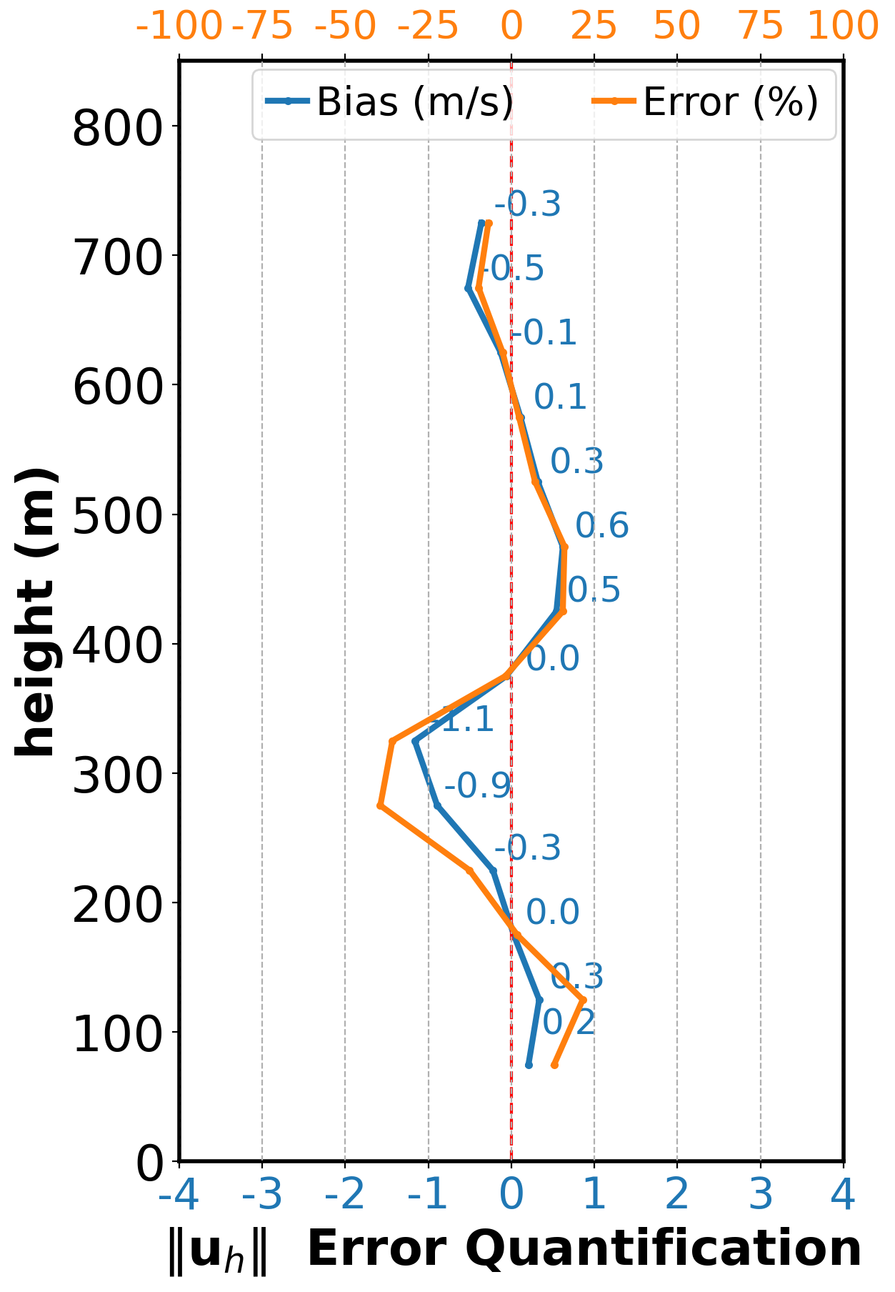
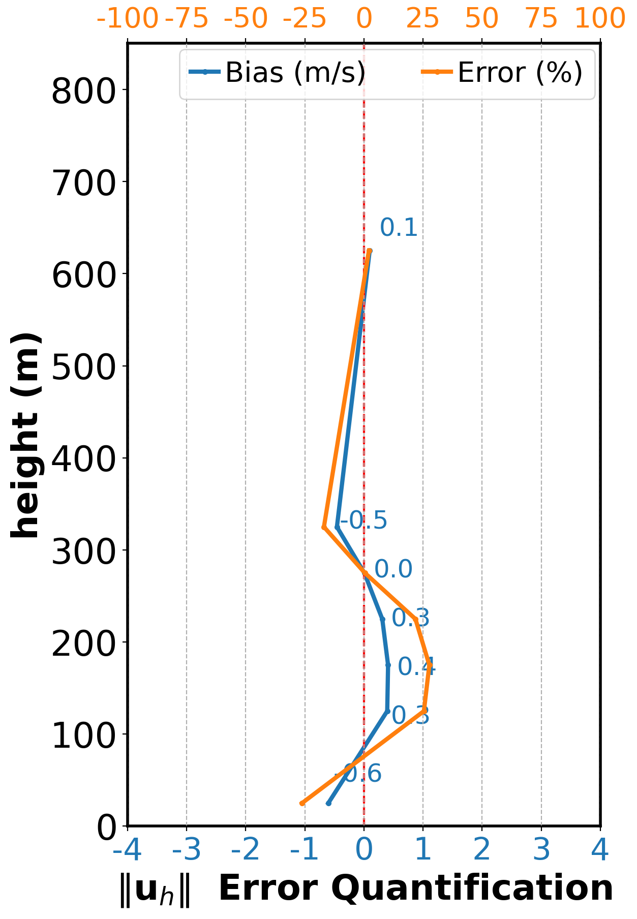
As for Case 3 shown in Figure 13, lidar data are further allocated to observation processing from data assimilation, and the overall verification metrics exhibit additional improvement. In comparison between the GAW105 wind profiler and the model simulations, the absolute errors are further reduced to within 0.3 m/s, with only the 300–400 m altitude range exhibiting a bias reaching approximately 0.5 m/s. For GAW110, except for a slightly larger discrepancy at the lowest observation level of the Doppler wind lidar, errors at all other heights remain below 0.5 m/s. Observed wind speed distribution by GAW110 in Figure 13(b) indicates that it records a wind speed of 2.3 m/s at the lowest level (approximately 50 m above ground), which decreases to 1.5 m/s with increasing height to 150 m. This vertical variation differs from the trends observed by other instruments. A preliminary assessment suggests that, at this particular instant, the observational instrument might have been influenced by external environmental factors or other interfering elements. Overall, all three validation sites demonstrate a satisfactory level of agreement. This consistency indicates that, in practical low-level wind field support events, low-level wind field computation and validation can be conducted with a sufficient level of confidence.


(a)

(b)

(c)


(d)
Case 4 further reduces the number of inputs to 2 lidars, while simultaneously expanding the spatial extent of the evaluation domain. Validation is conducted over four locations, including GAW104, GAW105, GAW110, and GAW111. The results shown in Figure 14 demonstrate that the simulations in all four regions are able to stably reproduce the vertical variation trends of the wind field. However, compared to Case 3, both the mean and maximum values of the overall error have increased slightly. This indicates that when observations from the two radars are used as model inputs, there is insufficient boundary information, leading to a decline in the accuracy of the simulation results. Although this validation method provides more comparative locations and attempts to reduce uncertainty, the accuracy of the simulation itself is compromised due to the reduction in effective data assimilation.
Among the four cases, Case 3 exhibits the highest degree of consistency in the validation results while providing enough validation locations. Therefore, an appropriate partitioning of observational data into subsets used for boundary-condition construction and for independent validation can effectively reduce the uncertainty in low-level wind-field prediction. Nevertheless, this does not necessarily imply an improvement in the absolute accuracy of the simulated results.
To quantitatively evaluate model performance at the lidar validation sites, we computed two coefficients of determination for each case based on the paired bin-averaged wind-speed samples from the withheld lidar observations and the corresponding model results:
| (5) |
| (6) |
Here, is the -th bin-averaged observed wind speed from the validation lidar data, is the corresponding simulated wind speed, is the total number of paired validation samples for the considered case, is the mean of all observed samples, and is the mean of all simulated samples. measures the reduction in residual variance relative to the variance of the observations, whereas is the square of the Pearson correlation coefficient and measures the linear agreement between simulations and observations. In computation, these two metrics were evaluated from the complete set of paired validation samples for each case.
The resulting values are summarized in Table 3. All cases exhibit consistently high agreement between the simulated and observed wind-speed profiles, with Case 3 achieving the highest scores under both metrics.
| Metrics | Case 1 | Case 2 | Case 3 | Case 4 |
| 0.874 | 0.875 | 0.947 | 0.919 | |
| 0.920 | 0.901 | 0.955 | 0.923 |
Moreover, even by using only a limited amount of sparse observational data as input, this set of experiments successfully infers both the vertical structure and the quantitative characteristics of the wind field in other regions. These results effectively demonstrate that the proposed simulation framework possesses strong capability for wind-field analysis and reconstruction under complex underlying surfaces with dense building coverage.
5 Conclusions
In this study, we develop and validate a lattice Boltzmann method with large-eddy simulation (LBM-LES) framework that leverages sparse station observations to reconstruct urban wind fields with near-real-time updates and continuous spatial coverage for low-altitude applications. The primary conclusions are as follows:
-
1.
Based on LBM-LES, our LatticeUrbanWind efficiently handles low-altitude wind field simulations, considering three-dimensional complex flow patterns, including building-induced flow, street canyon, and terrain influences.
-
2.
The synergistic integration of lidar and LBM-LES technology provides an effective solution for full spatial and temporal coverage of urban micrometeorological winds.
-
3.
The numerical results by the developed LBM-LES pipeline show good agreement with observations, demonstrating its accuracy and reliability. Within minutes, it completes meter-level resolution GPU-accelerated wind field simulations spanning several kilometers.
-
4.
The grid strategy exerts a pronounced influence on the simulation outcomes. In the present urban setting, 5 m is the coarsest tested resolution that still preserves the essential building geometry and near-ground profile structure, whereas coarser grids underestimate ground shear stress and yield an underdeveloped wind-velocity profile.
-
5.
The size of the precursor domain determines whether the flow is fully developed at the location of the focus region. A sufficiently large precursor domain provides an adequate buffer zone, enabling the reconstruction of turbulent characteristics. Moreover, the buffer length required for flow development is strongly influenced by the building density.
In summary, this paper presents a comprehensive verification and analysis of near-real-time simulation of low-altitude micrometeorological winds with CPU-GPU hybrid LBM-LES approach. We have deployed the platform to support low-altitude operations during major national events in China. Based on our existing findings, our subsequent research will further focus on the influence of multi-physics field coupling at the LBM drive boundary, including explicit treatment of vertical-velocity information, thermal (buoyancy) effects [62, 34] and high-order turbulent fields. Moreover, we are to establish standardized workflows, datasets and benchmarks for numerical simulations in urban environments, comparative to the open-access AIJ Wind Tunnel Database and Guideline [57, 41], in order to reduce the barrier to entry for new users and peers, and promote repeatability in continuously operating low-altitude support systems.
Declarations
-
1.
Funding:
This work was supported by Jing-Jin-Ji Regional Integrated Environmental Improvement - National Science and Technology Major Project (2025ZD1201
902) and Guangzhou Low-Altitude 628 Flight Meteorological Support Volunteer Observation Experiments Scheme. -
2.
Conflicts of interest:
The authors have no conflicts of interest to declare that are relevant to the content of this article. -
3.
Data availability:
Data supporting the findings of this study are available from the corresponding author on a reasonable request. Our LatticeUrbanWind platform is made open-source permanently under a customized non-commercial license and maintained at https://github.com/hweifluids/LatticeUrbanWind. The release version used in this study is LUW-v2.8. The necessary files to reproduce a complete end-to-end computational process are included to enhance usability and reproducibility.
References
- [1] (2010) Lattice-boltzmann method for complex flows. Annual Review of Fluid Mechanics 42, pp. 439–472. External Links: Document Cited by: §1.
- [2] (2015) The quiet revolution of numerical weather prediction. Nature 525, pp. 47–55. External Links: Document Cited by: §1, §1.
- [3] (2021) Designing airspace for urban air mobility: a review of concepts and approaches. Progress in Aerospace Sciences 125, pp. 100726. External Links: Document Cited by: §1.
- [4] (2013) Micro-scale pollutant dispersion modelling for the built environment. Building and Environment 64, pp. 1–2. External Links: Document Cited by: §1, §1.
- [5] (2014) 50 years of computational wind engineering: past, present and future. Journal of Wind Engineering and Industrial Aerodynamics 129, pp. 69–102. External Links: Document Cited by: §1, §1, §1, §3.
- [6] (2015) Computational fluid dynamics for urban physics: importance, scales, possibilities, limitations and ten years of progress. Building and Environment. External Links: Document Cited by: §1, §1, §1.
- [7] (2010) Urban greening to cool towns and cities: a systematic review of the empirical evidence. Landscape and Urban Planning 97 (3), pp. 147–155. External Links: Document Cited by: §1.
- [8] (2026) Estimating the impacts of the wind field size, wind speed, turbulence, and no-fly zones on unmanned aerial vehicle flights in urban areas. Physics of Fluids 38 (1), pp. 015130. External Links: Document Cited by: §1.
- [9] (2024) 3D-GloBFP: the first global three-dimensional building footprint dataset. Earth System Science Data 16 (11), pp. 5357–5374. External Links: Document Cited by: §3.
- [10] (2009) Large eddy simulations: how to evaluate resolution. International Journal of Heat and Fluid Flow 30 (5), pp. 1016–1025. Note: The 3rd International Conference on Heat Transfer and Fluid Flow in Microscale External Links: ISSN 0142-727X, Document Cited by: §4.1.
- [11] (2021) Urban air mobility: a comprehensive review and comparative analysis with autonomous and electric ground transportation for informing future research. Transportation Research Part C: Emerging Technologies 132, pp. 103377. External Links: Document Cited by: §1, §1.
- [12] (2006) Cascaded digital lattice boltzmann automata for high reynolds number flow. Physical Review E 73, pp. 066705. External Links: Document Cited by: §1.
- [13] (2022-10) Atmospheric flow simulation strategies to assess turbulent wind conditions for safe drone operations in urban environments. Journal of Wind Engineering and Industrial Aerodynamics 229, pp. 105136. External Links: Document Cited by: §1.
- [14] (1999) Aerodynamic properties of urban areas derived from analysis of surface form. Journal of Applied Meteorology 38 (9), pp. 1262–1292. External Links: Document Cited by: §1, §1, §1, §1.
- [15] (2023) CIM-powered physics-based assessment of wind damages to building clusters considering trees. Developments in the Built Environment 15, pp. 100178. External Links: Document Cited by: §1.
- [16] (2002-06) An extrapolation method for boundary conditions in lattice Boltzmann method. Physics of Fluids 14 (6), pp. 2007–2010. External Links: Document Cited by: §4.2.
- [17] (2002) Discrete lattice effects on the forcing term in the lattice boltzmann method. Physical Review E 65 (4), pp. 046308. External Links: Document Cited by: Appendix E.
- [18] (2019) Lattice boltzmann method-based large-eddy simulation of indoor isothermal airflow. International Journal of Heat and Mass Transfer 130, pp. 700–709. External Links: ISSN 0017-9310, Document Cited by: §1.
- [19] (2020) Validation of lattice boltzmann method-based large-eddy simulation applied to wind flow around single 1:1:2 building model. Journal of Wind Engineering and Industrial Aerodynamics 206, pp. 104277. External Links: ISSN 0167-6105, Document Cited by: §1, §4.1.
- [20] (2021) Effects of wall function model in lattice boltzmann method-based large-eddy simulation on built environment flows. Building and Environment 195, pp. 107764. External Links: ISSN 0360-1323, Document Cited by: §1.
- [21] (2010) Implementation of on-site velocity boundary conditions for D3Q19 lattice Boltzmann. Journal of Statistical Mechanics: Theory and Experiment 2010 (01), pp. P01018. External Links: Document Cited by: §4.2.
- [22] (2017) Large-eddy simulations over germany using ICON: a comprehensive evaluation. Quarterly Journal of the Royal Meteorological Society 143 (702), pp. 69–100. External Links: Document Cited by: §4.2.
- [23] (2026) Predicting urban wind extreme with gpu-accelerated lbm-les simulation and statistical method. Urban Climate 65, pp. 102746. External Links: ISSN 2212-0955, Document Cited by: §1.
- [24] (2026) Ten questions concerning urban wind environments for the safe utilization of urban air mobility. Building and Environment 290, pp. 114136. External Links: ISSN 0360-1323, Document Cited by: §1.
- [25] (2008) Outflow boundary conditions for the lattice Boltzmann method. Progress in Computational Fluid Dynamics, An International Journal 8 (1-4), pp. 38–48. External Links: Document Cited by: §4.2.
- [26] (2021) Palabos: parallel lattice boltzmann solver. Computers & Mathematics with Applications 81, pp. 334–350. External Links: Document Cited by: §1, §1.
- [27] (2022-07) Accuracy and performance of the lattice boltzmann method with 64-bit, 32-bit, and customized 16-bit number formats. Physical Review E 106, pp. . External Links: Document Cited by: Appendix D.
- [28] (2023) A comprehensive morphological classification scheme for local ventilation performance zones in spatially heterogeneous urban areas. Developments in the Built Environment 15, pp. 100202. External Links: Document Cited by: §1.
- [29] (2024) Open boundary conditions for atmospheric large-eddy simulations and their implementation in DALES4.4. Geoscientific Model Development 17 (9), pp. 4053–4076. External Links: Document Cited by: §4.2.
- [30] (2021) Turbulent channel flow simulations using the lattice boltzmann method with near-wall modeling on a non-body-fitted cartesian grid. Computers & Mathematics with Applications 93, pp. 20–31. External Links: ISSN 0898-1221, Document Cited by: §4.1.
- [31] (2002) An urban surface exchange parameterisation for mesoscale models. Boundary-Layer Meteorology 104, pp. 261–304. External Links: Document Cited by: §1, §1, §1.
- [32] (2000) A physically-based scheme for the urban energy budget in atmospheric models. Boundary-Layer Meteorology 94 (3), pp. 357–397. External Links: Document Cited by: §1, §1, §1.
- [33] (2017) Nested mesoscale-to-LES modeling of the atmospheric boundary layer in the presence of under-resolved convective structures. Journal of Advances in Modeling Earth Systems 9 (4), pp. 1795–1810. External Links: Document Cited by: §4.2, §4.2.
- [34] (2022) Urban buoyancy-driven air flow and modelling method: a critical review. Building and Environment 210, pp. 108708. External Links: ISSN 0360-1323, Document Cited by: §5.
- [35] (2000) Scale-invariance and turbulence models for large-eddy simulation. Annual Review of Fluid Mechanics 32, pp. 1–32. External Links: Document Cited by: §1, §1.
- [36] (2013) The response of the dines anemometer to gusts and comparisons with cup anemometers. Journal of Atmospheric and Oceanic Technology 30 (7), pp. 1320–1336. External Links: Document Cited by: §1.
- [37] (2007) Examining two-way grid nesting for large eddy simulation of the PBL using the WRF model. Monthly Weather Review 135 (6), pp. 2295 – 2311. External Links: Document Cited by: §4.2.
- [38] (2013) Sensors and the city: a review of urban meteorological networks. International Journal of Climatology 33 (7), pp. 1585–1600. External Links: Document Cited by: §1, §1.
- [39] (2018) Evaluation of k- reynolds stress modeling in an idealized urban canyon using les. Journal of Wind Engineering and Industrial Aerodynamics 175, pp. 213–228. External Links: Document Cited by: §1.
- [40] (2021) NASADEM global digital elevation model. OpenTopography. Note: Accessed 2025-11-11 External Links: Document Cited by: §3.
- [41] (2026) AIJ guidelines on the applications of large-eddy simulation to pedestrian wind environment: recommendations and validation benchmarks. Journal of Wind Engineering and Industrial Aerodynamics 269, pp. 106321. External Links: ISSN 0167-6105, Document Cited by: §5.
- [42] (2021) Large-eddy simulation of flow around an isolated building: a step-by-step analysis of influencing factors on turbulent statistics. Building and Environment 202, pp. 108021. External Links: ISSN 0360-1323, Document Cited by: §1.
- [43] (1988) Street design and urban canopy layer climate. Energy and Buildings 11, pp. 103–113. External Links: Document Cited by: §1.
- [44] (2015) A review on regional convection-permitting climate modeling: demonstrations, prospects, and challenges. Bulletin of the American Meteorological Society 96 (12), pp. 2027–2047. External Links: Document Cited by: §1.
- [45] (2021) Sensitivity of organized convective storms to model grid spacing in current and future climates. Philosophical Transactions of the Royal Society A: Mathematical, Physical and Engineering Sciences 379 (2195), pp. 20190546. External Links: Document Cited by: §1.
- [46] (2021) An initial assessment of the potential weather barriers of urban air mobility. IEEE Transactions on Intelligent Transportation Systems. External Links: Document Cited by: §1, §1, §1.
- [47] (2008) Scale-selective verification of rainfall accumulations from high-resolution forecasts of convective events. Monthly Weather Review 136 (1), pp. 78–97. External Links: Document Cited by: §1.
- [48] (2019) Kilometer-scale climate models: prospects and challenges. Bulletin of the American Meteorological Society. External Links: Document Cited by: §1, §1, §1.
- [49] (2016) Massively parallel algorithms for the lattice boltzmann method on nonuniform grids. SIAM Journal on Scientific Computing 38 (2), pp. C96–C126. External Links: Document Cited by: §1.
- [50] (2009) Next-day convection-allowing wrf model guidance: a second look at 2-km versus 4-km grid spacing. Monthly Weather Review 137 (10), pp. 3351–3372. External Links: Document Cited by: §1.
- [51] (2024) Evaluation of multi-layer urban canopy model (mlucm) for urban microclimate predictions at different urban contexts. Urban Climate 55, pp. 101882. External Links: ISSN 2212-0955, Document Cited by: §1.
- [52] (2019) Urban air mobility: opportunities for the weather community. Bulletin of the American Meteorological Society 100 (11), pp. 2131–2133. External Links: Document Cited by: §1, §1, §1.
- [53] (2025) A fast and automated approach for urban cfd simulations: validation with meteorological predictions and its application to drone flights. Urban Climate 64, pp. 102664. External Links: ISSN 2212-0955, Document Cited by: §1.
- [54] (2025) Climate sensitive designs for policy makers: how les model resolution affects accuracy in capturing urban micro-scale weather during heatwaves. Urban Climate 61, pp. 102400. External Links: ISSN 2212-0955, Document Cited by: §4.1.
- [55] (2025) Advancing low-carbon smart cities: leveraging uavs-enabled low-altitude economy principles and innovations. Renewable and Sustainable Energy Reviews 222, pp. 115942. External Links: Document Cited by: §1.
- [56] (2020) An analytical review on the evaluation of wind resource and wind turbine for urban application: prospect and challenges. Developments in the Built Environment 4, pp. 100033. External Links: Document Cited by: §1.
- [57] (2008) AIJ guidelines for practical applications of cfd to pedestrian wind environment around buildings. Journal of Wind Engineering and Industrial Aerodynamics 96 (10), pp. 1749–1761. External Links: Document Cited by: §1, §1, §1, §5.
- [58] (2003) Modelling air quality in street canyons: a review. Atmospheric Environment 37 (2), pp. 155–182. External Links: Document Cited by: §1.
- [59] (2000) Evaluation of two gustiness models for exposure correction calculations. Journal of Applied Meteorology 39 (9), pp. 1613–1626. External Links: Document Cited by: §1.
- [60] (2025) Exploration of computational formulations for wind-induced interference effects on high-rise buildings via Kolmogorov–Arnold networks. Developments in the Built Environment 24, pp. 100770. External Links: Document Cited by: §1.
- [61] (2024-11) EVTOL flys through atmospheric boundary layer: unsteady take-off and landing study via spatio-temporal projection method. In SAE 2024 Intelligent Urban Air Mobility Symposium, External Links: Document Cited by: §1.
- [62] (2024) Exploring thermal buoyant flow in urban street canyons: influence of approaching turbulent boundary layer. Experimental Thermal and Fluid Science 158, pp. 111255. External Links: ISSN 0894-1777, Document Cited by: §5.
- [63] (2025-08) A review of airborne doppler lidar for wind-sensing. Progress in Aerospace Sciences 157, pp. 101127. External Links: Document Cited by: §1.
- [64] (2025) TH-music: a high-performance multi-scale nwp-lbm coupling framework with cpu–gpu architecture for high-fidelity real-time urban wind field simulation. Building and Environment 283, pp. 113313. External Links: ISSN 0360-1323, Document Cited by: §1, §1.
- [65] (2025) The impact of low-altitude airspace opening policy on aviation manufacturing innovation: a double machine learning approach. Transportation Research Part A: Policy and Practice 200, pp. 104660. External Links: Document Cited by: §1.
- [66] (2025) Unmanned aerial vehicles based low-altitude economy with lifecycle techno-economic-environmental analysis for sustainable and smart cities. Journal of Cleaner Production 499, pp. 145050. External Links: Document Cited by: §1.
- [67] (1997-06) On pressure and velocity boundary conditions for the lattice Boltzmann BGK model. Physics of Fluids 9 (6), pp. 1591–1598. External Links: Document Cited by: §4.2.
Appendix A Kriging boundary construction from lidar
This appendix describes a deterministic procedure for converting quality-controlled Doppler lidar profile observations into gridded three-dimensional horizontal wind fields to be used as boundary forcing in numerical simulations. At each analysis time , the method combines multi-site lidar samples, performs layer-wise spatial interpolation using Ordinary Kriging in the horizontal plane, and stacks the resulting fields across prescribed height levels to form on a regular grid.
For a target time , the nearest available profile file at each lidar site is selected under a temporal tolerance of minutes relative to . Within each selected file, samples are filtered to retain heights and quality-control flags indicating pass. Each retained sample is represented as , where denotes the site longitude and latitude, is the sample height, and is the wind vector. Samples from all sites are merged into a single set . If fewer than three distinct sites are available at time , a deterministic augmentation is applied by replicating the merged sample set and adding a small, fixed perturbation to longitudes, latitudes, and wind components to prevent singular Kriging systems; this step is only used to ensure numerical solvability under severe data sparsity and does not introduce stochasticity.
The horizontal computational domain is defined in longitude–latitude space, and a regular grid is generated with spacing . The vertical coordinate is discretized by a set of target levels , typically spanning – with an increment of . The three-dimensional target grid is therefore .
To avoid fitting and solving a full three-dimensional covariance model, interpolation is performed independently at each target height . For a given , a layer-specific subset is formed as
which collects samples within a symmetric height tolerance window around . For each wind component, Ordinary Kriging is applied only when a sufficient number of samples is available in ; otherwise, the corresponding grid values at height are left as missing.
At a fixed height , let denote the horizontal location of the -th sample and let denote the observed value of a wind component . Ordinary Kriging assumes an unknown but constant mean over the local domain and estimates the value at a target location as a weighted sum
where and are weights chosen to ensure unbiasedness and minimum estimation variance. The weights are obtained by solving the Kriging linear system written in terms of the semivariogram :
where is a Lagrange multiplier enforcing the unbiasedness constraint. The resulting estimate is evaluated on all grid points to form the layer field , and the procedure is applied separately to and .
The semivariogram model is chosen as the spherical form
where is the nugget, is the sill, and is the range parameter controlling the spatial influence scale. For each height level and each wind component, an initial fit is obtained from the empirical semivariogram using a finite number of lag bins (eight bins). To avoid numerical degeneracy associated with vanishing nuggets, the nugget is lower-bounded by when the fitted value is smaller than . To ensure that observational influence extends to the computational domain edges, the range parameter is set to (consistent with the longitude–latitude coordinate units) for the final interpolation. The final Kriging evaluation uses a fixed lag-binning configuration employing six bins. This range control is the principal mechanism by which boundary values remain constrained by the observations rather than reverting to weakly informed extrapolations near the domain periphery.
For each time , the layer-wise interpolated fields are stacked over to obtain three-dimensional arrays . Height levels that are entirely missing are removed prior to output. The resulting boundary fields are stored in netCDF format with dimensions (height, lat, lon), using floating-point storage and lossless compression. The overall procedure is deterministic: given identical inputs, grid definitions, semivariogram model choices, and parameter rules (including nugget thresholding and enforced range), the Kriging solutions and outputs are uniquely reproducible.
Appendix B Construction of terrain layer
The terrain elevations are interpolated to the query point from -th grid points using inverse distance weighting (IDW):
| (7) |
where the IDW power parameter is , the index set of the nearest neighbors of is . A small constant prevents division-by-zero. Grid node coordinates are with grid values . Local normalized coordinates inside a grid cell are and . The base height used for building placement is . Then apply smoothing with discrete Gauss kernel to the resulting raster, and finally perform fast per-point lookups on that using bilinear interpolation on a precomputed grid:
| (8) |
where and are the local normalized coordinates, defined by
| (9) |
The lowest point of the building is aligned with the lowest point of the terrain at the extent of the base to avoid intersecting gaps. The final Boolean-merged voxelization consists of three layers, including a fixed-thickness base, terrain elevation, and a building layer.
According to the DEM raw data resolution and interest of terrain variations, the spatial resolution and smoothness parameters of terrain construction are user-adjustable.
Appendix C Velocity interpolation
The interpolation is done in two steps, first downscaling the boundary data to the hundred-meter level and then further down to the meter-level CFD grid, using different numerical methods to balance computational cost (efficiency) and numerical accuracy. Both of them are implemented in parallel. The irregular discrete point field distributed on the plane after projection and rotation, which are similar to the buildings and DEM database, is interpolated onto a Cartesian grid whose origin is known and whose spacings are uniform in both directions. The original discrete point set is first used to construct a Delaunay triangulation on the plane, so that the entire planar region is partitioned into a number of triangular elements composed of the original observation points. It is further assumed that within each triangle the physical quantity can be regarded geometrically as linearly approximable. The complete set of nodes on the target regular grid is then generated, namely the regular node set formed by the Cartesian product of the equally spaced x sequence and the equally spaced y sequence. For a target node, the coordinates of the three vertices of the triangle containing this node are extracted, and the affine transformation stored in the triangulation structure is employed to map the target node into the barycentric coordinate system of that triangle. For the mapping yields two barycentric parameters and , the third barycentric weight is given as . Let three weights correspond respectively to the physical quantities ,, at three vertices of the triangle, then the interpolated value is given by
| (10) |
Geometrically this is equivalent to treating the Delaunay triangles as linear finite elements and performing a single linear interpolation of the field inside each element, which preserves the local gradients of the original data and does not introduce additional smoothing. For target nodes that lie outside the convex hull of the triangulation, the algorithm reverts to nearest-neighbor interpolation. For this purpose a cKDTree is preconstructed for all original discrete points and used to perform nearest point queries.
After this interpolation, the boundary data is saved on an intermediate grid (O(100 m) spacing) and passed to the second-stage interpolator to construct the real boundary on the CFD mesh. For this purpose, two options are provided, choosing between faster and more continuous interpolation, including improved variant of KNN interpolation and basic nearest scheme. For this improved KNN method, the boundary samples are used to reconstruct the inlet velocity on the CFD boundary during initialization. In this second stage, the interpolator is evaluated pointwise on the CFD boundary grid, while enforcing a vertical cutoff. Specifically, for any query location , the inlet velocity is set to zero when , and only the remaining locations are passed to the surface interpolator.
The interpolation is performed in a surface consistent manner by explicitly assigning each query point to a unique boundary face before any neighborhood search. Let denote the axis aligned bounding box of the sample coordinates. The query point is associated with the closest plane among the five candidate faces by minimizing the absolute distance to these planes. Only samples lying on the selected face are retained, using a tolerance
| (11) |
which suppresses cross face contamination near edges and corners.
After the face is determined, distances are computed in the local two dimensional coordinates intrinsic to that face, rather than in the full three dimensional space. For a sample point and query point , the local offsets are defined by
| (12) |
and the squared in plane distance is
| (13) |
The nearest samples on the assigned face are selected according to . A Gaussian kernel is then used to define weights,
| (14) |
where denotes the selected neighborhood, and is lower bounded to avoid degeneracy. Using these weights, each velocity component is reconstructed by a weighted quadratic surface fit on the local coordinates,
| (15) |
with the coefficients obtained from the corresponding weighted normal equations. Since the local coordinates are centered at the query point, the interpolated velocity equals the constant term of the fitted polynomial for each component, which yields a smooth surface based inlet reconstruction that is consistent with the boundary face ownership and the imposed height threshold.
Appendix D Lattice Boltzmann method in FluidX3D
Developed by Lehmann [27], FluidX3D is an OpenCL-based GPU-accelerated LBM solver, excelling in extreme computational efficiency. We customize and integrate it in the LatticeUrbanWind workflow as the LBM-LES component, optimizing from the perspectives of ray-tracing voxelization, boundary treatment, and lightweight construction.
The weakly-compressible lattice Boltzmann method (LBM) is employed to numerically solve a kinetic-equivalent system of the incompressible Navier–Stokes equations in the low-Mach-number limit. In LBM, a set of distribution functions is introduced at each lattice node over a discrete velocity set , and macroscopic fields are recovered through discrete velocity moments. The D3Q19 model denotes 19 discrete velocity directions in three-dimensional space; the associated weights and lattice sound speed satisfy isotropy constraints for and tensor moments. In lattice units, the sound speed is . The macroscopic density and velocity are given by the and moments
| (16) |
The pressure is related to the density through the equation of state . By a Chapman–Enskog multiscale expansion, under low-Mach and near-equilibrium conditions, the macroscopic limit of LBM is consistent with the incompressible Navier–Stokes equations, with the viscous term controlled by the collision relaxation time.
An SRT BGK collision operator is adopted. Each time step consists of a local collision followed by lattice streaming. The discrete evolution can be written as
| (17) |
| (18) |
Here is the effective relaxation time, which is a spatiotemporally varying quantity in the LES branch; denotes the equilibrium distribution function.
The equilibrium distribution is taken in the second-order Hermite-truncated form with the velocity as a small parameter
| (19) |
This expression satisfies the moment constraints required for mass and momentum conservation and provides a second-order accurate approximation of the convective term in the low-Mach-number regime.
In SRT-LBM, the relation between the kinematic molecular viscosity and the relaxation time is
| (20) |
where is the relaxation time in the absence of a subgrid-scale model and is the molecular viscosity. The LES branch incorporates unresolved momentum transport through an eddy-viscosity concept. The effective viscosity is defined as
| (21) |
where is the subgrid eddy viscosity. The Smagorinsky–Lilly model is given by
| (22) |
with the model constant, the filter scale, and the strain-rate tensor.
To maintain a fully local formulation, the strain rate is not obtained via explicit spatial differencing of the velocity field, but is constructed from the nonequilibrium second-order moment. Define the nonequilibrium momentum-flux tensor
| (23) |
which relates to the strain rate as
| (24) |
Further define the tensor invariant
| (25) |
By combining with , a closed-form expression for is obtained. The explicit solution is
| (26) |
so that can be computed at each lattice node from the local distribution functions and then substituted into the BGK collision step to introduce subgrid dissipation. This construction preserves the conservative structure and locality of the SRT-LBM while realizing the LES closure.
For the no-slip wall boundary on the buildings, it is enforced via mid-grid (halfway) bounce-back at fluid–solid links, with solid cells defined by a voxel mask, which is determined by a improved ray-tracing kernel by us. The wall is located half a lattice spacing from the adjacent fluid cell, and populations directed into the solid are reflected into the opposite lattice direction, yielding a stationary no-slip condition at the boundary. With pull-based in-place streaming (Esoteric-Pull), this bounce-back is realized implicitly within the stream–collide kernel.
Appendix E Coriolis forcing term
The Coriolis acceleration in a rotating frame is given by , where is the Earth’s angular velocity vector and is the local velocity recovered from the distribution functions in LBM. The source term is assembled within the device kernel immediately after reconstruction of the macroscopic fields to avoid host-to-device copy costs. For geophysical flows it is convenient to express the Coriolis term by means of the Coriolis frequency where is the latitude of the computational domain and is the magnitude of the Earth’s rotation rate, taking . In the present implementation, the Earth rotation vector is first projected from the Earth centred frame into the local east-north-up (ENU) frame at latitude :
| (27) |
These three components, expressed in the local frame, are passed from the host to the device together with the other run time parameters. In this way the kernel can construct the Coriolis volume force without performing additional geometric operations. Because the LBM is formulated in a nondimensional lattice unit system, the angular velocity components is nondimensionalized by
| (28) |
where denotes the physical grid spacing, is the nondimensional reference velocity, and is the corresponding reference velocity in SI units. Inside the GPU kernel, after recovering the density and velocity from the distribution functions, the Coriolis body force per unit volume is formed as
| (29) |
It is then supplied to the forcing source term routine that implements the Guo’s method [17]. Thereby, the Coriolis force is incorporated as a high accuracy source term within the LBM time stepping without introducing additional communication overhead or reducing numerical stability.
Appendix F Turbulence Generation Approach
Our turbulence generation module (von Karman inflow) is implemented as a GPU-based on-the-fly synthetic Fourier boundary condition acting on the equilibrium-boundary velocity field before each LBM time step. Let denote the set of active boundary cells used by the turbulence generator. In the present implementation, is assembled from the west, east, south, north, and top boundary planes; bottom cells are excluded to preserve the ground wall, solid cells are excluded, and only cells already marked as equilibrium boundaries are admitted. To avoid duplicate writes at shared edges and corners, each boundary node is assigned to one face only. An optional inflow filter further restricts the set to cells satisfying , where is the prescribed mean boundary velocity at cell and is the inward unit normal of face .
For each candidate face , the code first computes the face-mean velocity
| (30) |
and the face characteristic speed,
| (31) |
where the two alternatives correspond to the two characteristic-speed definitions implemented in the code. Faces with are discarded. The temporal convection of all modes is then based on global quantities gathered over all active inlet cells,
| (32) |
with the fallback only if the denominator vanishes. A separate random realization is normally constructed for each active face by mixing the base random seed with the face identifier, although the implementation also supports sharing one realization across all faces.
For each face, the fluctuating field is represented by a discrete random Fourier expansion,
| (33) |
where is the boundary-cell position in global lattice coordinates, is the number of modes, is the wave vector, is the temporal frequency, is an independent random phase, and is the component-wise modal amplitude. The wave-number magnitude is sampled in logarithmic space,
| (34) |
with , , and . In lattice units , so . If the requested band becomes degenerate, the implementation resets to to preserve a valid spectral interval. The wave-vector direction is sampled isotropically in three dimensions,
| (35) |
and .
The von Karman spectral shape is introduced through the raw modal weight
| (36) |
where is the prescribed integral length scale in lattice units. The raw amplitudes are normalized by
| (37) |
so that each Cartesian component of the unscaled synthetic field has unit RMS because . Optional anisotropy is introduced afterward through independent component gains,
| (38) |
This means that anisotropy is implemented in a purely component-wise manner: the same discrete von Karman spectrum , the same wave-number sampling, and the same convection frequency are used for all three components, while only their amplitudes are rescaled. Consequently, before the local factor is applied, the RMS level of each component is proportional to , , and , respectively. In other words, the present implementation realizes variance anisotropy rather than anisotropic length scales or an anisotropic wave-vector distribution. No explicit solenoidal projection is applied, i.e., the construction does not enforce at the synthetic-field level; instead, it injects a statistically shaped perturbation through the boundary velocities and leaves the subsequent flow adjustment to the LBM evolution.
The modal time dependence follows a frozen-convection assumption,
| (39) |
which convects all Fourier modes along the global mean-flow direction. The perturbation amplitude is then scaled locally at each boundary cell as
| (40) |
where is the prescribed turbulence intensity, is a constant fallback fluctuation level, and are the component-wise anisotropy gains. The final boundary velocity imposed on cell is
| (41) |
Hence, the synthetic turbulence is superposed on the pre-existing mean boundary field rather than replacing it.
When a temporal stride is used, the synthetic field is evaluated from anchor times . The implementation then either holds the field piecewise constant at , or linearly interpolates between two anchors,
| (42) |
Numerically, our code gathers all active inlet cells once, maps them to the owning GPU subdomains, and stores cell indices, face identifiers, global lattice coordinates, base velocities, and local values in structure-of-arrays buffers. The mode tables are stored in the same format. During the simulation, one GPU thread is launched per active inlet cell; that thread loops over the modes of its face, evaluates the cosine series at the current time, and overwrites the boundary velocity array before the subsequent LBM update. Because phase evaluation uses global lattice coordinates, the realization remains consistent across domain decomposition boundaries without storing a precomputed turbulent inflow history.
Appendix G 2D Wavenumber Spectra
