Regularized Projection Algorithms for Monotone Inverse Variational Inequalities
Griffin Smith, Zeinab Alizadeh, Afrooz Jalilzadeh

Abstract

Stochastic inverse variational inequalities (SIVIs) arise in applications in which equilibrium responses are observed under uncertainty, such as inverse road pricing and network equilibrium control. Existing methods typically rely on co-coercivity or strong monotonicity, while general monotone SIVIs remain less understood. We propose a regularized projection algorithm that combines Tikhonov regularization with increasing batch sizes. Under monotonicity and Lipschitz continuity, we prove almost sure boundedness of the iterates and almost sure convergence of their distance to the SIVI solution set. We further establish, to the best of our knowledge, the first explicit nonasymptotic rate of $O(T^{-1/2})$ for the expected squared residual under general monotonicity. This yields $O(\epsilon^{-2})$ iterations and $O(\epsilon^{-4-2\delta})$ stochastic oracle calls, for any $\delta>0$, to obtain an $\epsilon$-solution in expected squared residual. A deterministic variant attains the same iteration complexity using $O(\epsilon^{-2})$ exact operator evaluations. Numerical experiments illustrate the proposed methods on monotone SIVI problems.

1 Introduction

Interest in Inverse Variational Inequalities (IVIs) has grown significantly in recent decades [9], driven by their broad applicability across diverse domains such as transportation system operation, the formulation of control policies, and electrical power network management [24, 11, 21, 10]. In this paper, we focus on Stochastic Inverse Variational Inequalities (SIVI). In particular, let $X\subseteq\mathbb{R}^{n}$ be a nonempty closed convex set, and $F:\mathbb{R}^{n}\to\mathbb{R}^{n}$ be a continuous nonlinear map. In the SIVI problem, we seek $x^{*}\in\mathbb{R}^{n}$ such that $F(x^{*})\in X$ and

$$\langle y-F(x^{*}),x^{*}\rangle\geq 0,\quad\forall y\in X,$$ (SIVI)

where $F(x)\triangleq\mathbb{E}[G(x,\xi)]$, $\xi:\Omega\to\mathbb{R}^{d}$, ${G}:\mathbb{R}^{n}\times\mathbb{R}^{d}\rightarrow\mathbb{R}^{n}$, and the associated probability space is denoted by $(\Omega,{\cal F},\mathbb{P})$. The SIVI framework seeks a solution $x^{*}$ that satisfies a specific system of inequalities across the entire feasible set $X$. When $F^{-1}$ is single-valued and well defined on $X$, the SIVI is mathematically equivalent to a Stochastic Variational Inequality (SVI) defined by $H\triangleq F^{-1}$; however, the inverse mapping is often unavailable or computationally expensive to evaluate, necessitating the development of “inverse-free” iterative schemes. While VIs [19, 7, 17, 3] and SVIs [13, 14, 25, 12, 1] have been studied extensively, the study of IVIs and SIVIs is still underdeveloped. In the deterministic setting, approximation methods have been developed for IVIs under assumptions such as strong monotonicity and co-coercivity. These approaches include proximal point-based algorithms, projection-type methods, alternating contraction projection methods, and dynamical system methods [22, 6, 23, 5, 16]. Specifically, projection-based algorithms were pioneered by [11, 10, 16], and [26] introduced neural network-based methods to approximate solutions. To ensure stability in deterministic and monotone settings without stronger structural assumptions such as strong monotonicity or co-coercivity, Anh and Hai [4] extended the regularized iterative framework of [15] by proposing a regularized dynamical system for monotone IVIs in Hilbert spaces. Their approach admits a unique strong global solution and establishes strong convergence under relatively mild assumptions. However, despite these stability and asymptotic convergence guarantees, explicit nonasymptotic convergence rate results remain unavailable. In the stochastic domain, research is even more sparse. In [2], a variance-controlled projection-based algorithm was developed specifically for SIVIs when the operator is co-coercive. They established almost sure convergence of the generated iterates to the solution and provided a convergence rate guarantee of $\mathcal{O}(1/T)$, which stands as a benchmark for the co-coercive class of problems. However, co-coercivity is a restrictive assumption that may not hold for general monotone mappings. Despite these advancements, an explicit convergence rate for the general monotone SIVIs remains unavailable in the current literature to the best of our knowledge.

1.1 Applications

IVIs arise in transportation, network economics, power systems, and other equilibrium-control problems, where the goal is to choose a control vector whose induced equilibrium response satisfies prescribed constraints. In stochastic settings, this response is represented by the mean map $F(x):=\mathbb{E}[G(x,\xi)]$. We next present two representative SIVI formulations.

Inverse Road Pricing Problem: Road pricing is a classical traffic-management tool used to regulate congestion and achieve operational or environmental targets [24]. In a standard traffic-equilibrium problem, the toll vector is fixed and the corresponding user-equilibrium flow is determined according to Wardrop’s principle. In contrast, an inverse road-pricing problem seeks a toll vector that induces a desirable equilibrium flow pattern. This interpretation is consistent with the black-box IVI framework in [11], in which the toll-to-flow response can be computed approximately even when its inverse is unavailable.

Consider a network with $n$ controlled links, and let $x\in\mathbb{R}^{n}$ denote the vector of link tolls. For a given toll vector $x$, let $a^{*}(x)\in\mathbb{R}^{n}$ denote the induced equilibrium link-flow vector. The set of admissible flow patterns may be defined as $X:=\{a\in\mathbb{R}^{n}\mid\underline{a}\leq Ca\leq\bar{a}\}$, where $C\in\mathbb{R}^{q\times n}$ is a selection or aggregation matrix and $\underline{a},\bar{a}\in\mathbb{R}^{q}$ specify flow, capacity, or environmental bounds. The stochastic inverse road-pricing problem can then be modeled as finding $x^{*}\in\mathbb{R}^{n}$ such that $F(x^{*})\in X$ and $\langle y-F(x^{*}),x^{*}\rangle\geq 0,$ for all $y\in X$. Here $G(x,\xi)$ denotes the stochastic equilibrium-flow response under toll vector $x$, where $\xi$ may represent random demand, incidents, weather, or measurement errors. For additive zero-mean measurement noise, one may write $G(x,\xi)=a^{*}(x)+\xi$, in which case $F(x)=a^{*}(x)$. Since the toll-to-flow mapping is generally available only through observations, simulations, or equilibrium computations, this formulation motivates stochastic inverse-free methods.

Resource-Constrained Network Equilibrium: Consider a commodity network with $m$ supply markets, $n$ demand markets, and $mn$ shipment routes. Let $a\in\mathbb{R}^{mn}_{+}$ denote the shipment vector and let $x=[x_{1}^{\top},x_{2}^{\top}]^{\top}\in\mathbb{R}^{m+n}$ denote a policy vector, where $x_{1}\in\mathbb{R}^{m}$ and $x_{2}\in\mathbb{R}^{n}$ represent supply- and demand-side tax adjustments. For a fixed policy $x$, the equilibrium shipment vector $a^{*}(x)$ is obtained from the parametric VI

$$\left\langle a^{\prime}-a,\,\ell(a)+A^{\top}\bigl(g(Aa)+\alpha+x_{1}\bigr)-B^{\top}\bigl(h(Ba)-\beta-x_{2}\bigr)\right\rangle\geq 0,$$ (1)

for all $a^{\prime}\in\mathbb{R}^{mn}_{+}$, where $A:=I_{m}\otimes e_{n}^{\top}\in\mathbb{R}^{m\times mn}$ and $B:=e_{m}^{\top}\otimes I_{n}\in\mathbb{R}^{n\times mn}$ aggregate shipments into supply and demand vectors. The mappings $\ell$, $g$, and $h$ represent transportation costs, supply prices, and demand prices, respectively, while $\alpha$ and $\beta$ denote baseline policy parameters. Define the induced aggregate response by $F(x):=[(Aa^{*}(x))^{\top},(Ba^{*}(x))^{\top}]^{\top}\in\mathbb{R}^{m+n}$, and let $X:=\{u\in\mathbb{R}^{m+n}\mid Lu\leq b\}$ denote the set of admissible aggregate supply-demand states. Following the constrained black-box IVI framework of [8], the regulator seeks $x^{*}\in\mathbb{R}^{m+n}$ such that $F(x^{*})\in X$ and $\langle v-F(x^{*}),x^{*}\rangle\geq 0,$ for all $v\in X$. Under uncertainty, the regulator observes a stochastic response $G(x,\xi)$ satisfying $\mathbb{E}[G(x,\xi)]=F(x)$. For example, under additive zero-mean observation noise, $G(x,\xi):=[(Aa^{*}(x)+\xi_{1})^{\top},(Ba^{*}(x)+\xi_{2})^{\top}]^{\top}$, where $\xi_{1}\in\mathbb{R}^{m}$ and $\xi_{2}\in\mathbb{R}^{n}$. Such network models provide a natural application of the proposed method whenever the resulting mean response is monotone and Lipschitz continuous but is not assumed to be co-coercive [18].

These examples involve controlling an equilibrium response observed through noisy data, simulations, or equilibrium computations. Since the inverse map may be unavailable and the mean response may be monotone but not co-coercive or strongly monotone, they motivate methods with guarantees for monotone SIVIs.

1.2 Contribution

Motivated by the lack of explicit convergence-rate guarantees for stochastic IVIs under general monotonicity, we propose the Regularized Variance-Controlled Inverse Projected Gradient (RVC-IPG) method, which combines Tikhonov regularization with increasing batch sizes to handle monotonicity and stochastic error without requiring co-coercivity or strong monotonicity. The closest related works are [4] and [2]. Anh and Hai [4] study deterministic monotone IVIs and establish asymptotic convergence, but no explicit nonasymptotic rate is provided. Our previous work [2] proves an $\mathcal{O}(1/T)$ rate for stochastic IVIs under co-coercivity; in contrast, the present paper removes co-coercivity and establishes an explicit $\mathcal{O}(T^{-1/2})$ residual rate under general monotonicity. Our contributions are threefold:

1. We develop an almost sure convergence theory for monotone SIVIs. We show that each regularized SIVI has a unique solution, the regularization path is bounded, and its limit points solve the SIVI. Building on these properties, we prove that the RVC-IPG iterates are almost surely bounded and their distance to the SIVI solution set converges to zero almost surely.

2. We establish an explicit nonasymptotic residual bound. For suitable choices of the stepsize, regularization, projection parameter, and batch size, we prove that $\min_{0\leq k\leq T-1}\mathbb{E}[|H(x_{k},\eta_{k})|^{2}]=O(T^{-1/2})$, where $H$ is the natural residual map associated with the inverse projection condition. This yields an $O(\epsilon^{-2})$ iteration complexity and an $O(\epsilon^{-4-2\delta})$ stochastic oracle complexity, for any $\delta>0$, to obtain an $\epsilon$-solution in expected squared residual. To the best of our knowledge, this is the first explicit nonasymptotic rate for stochastic inverse variational inequalities under general monotonicity, without co-coercivity or strong monotonicity of the mean operator.

3. We connect the rate result to practical residual evaluation and deterministic computation. We show that the same $O(T^{-1/2})$ rate holds for a fixed projection parameter, enabling consistent comparison across iterations in numerical experiments. We also analyze a deterministic counterpart of RVC-IPG and prove that it attains the same $O(\epsilon^{-2})$ iteration complexity using exact evaluations of the mean operator. Numerical experiments on SIVI instances that are monotone but not co-coercive illustrate the behavior of the proposed methods and support the theoretical findings.

2 Preliminaries

In this section, we first introduce notation and then state the main assumptions used in the convergence analysis.

Notation. Throughout the paper, $\|x\|$ denotes the Euclidean vector norm, i.e., $\|x\|=\sqrt{x^{T}x}$. $\mathbf{P}_{X}[u]$ is the projection of $u$ onto the set $X$, i.e. $\mathbf{P}_{X}[u]=\mbox{argmin}_{z\in X}\frac{1}{2}\|z-u\|^{2}$. $\mathbb{E}[x]$ is used to denote the expectation of a random variable $x$. For $\rho>0$, $B_{\rho}(x)$ denotes the closed ball of radius $\rho$ centered at $x$, i.e., $B_{\rho}(x)\triangleq\{z\in\mathbb{R}^{n}:\|z-x\|\leq\rho\}$.

Definition 1.

An operator $A:X\rightarrow\mathbb{R}^{n}$ is said to be

(i) $\mu$-strongly monotone if and only if there exists a constant $\mu>0$ such that $\langle A(x)-A(y),x-y\rangle\geq\mu\|x-y\|^{2}$ for all $x,y\in X.$

(ii) monotone if and only if $\langle A(x)-A(y),x-y\rangle\geq 0$ for all $x,y\in X.$

(iii) $L$-Lipschitz continuous if and only if there exists a constant $L>0$ such that $\|A(x)-A(y)\|\leq L\|x-y\|,$ for all $x,y\in X.$

Define $\mathcal{F}_{k}$ denotes the information history, i.e., $\mathcal{F}_{k}:=\sigma\{x_{0},\xi_{j,s}:0\leq s\leq k-1;1\leq j\leq N_{s}\},$ at epoch $k$. We impose the following assumption on the stochastic error.

$$\bar{w}_{k,N_{k}}\triangleq\tfrac{1}{N_{k}}{\sum_{j=1}^{N_{k}}(G(x_{k},\xi_{j,k})-F(x_{k}))}$$ (2)

Assumption 1.

There exists $\nu>0$ such that $\mathbb{E}[\bar{w}_{k,N_{k}}\mid\mathcal{F}_{k}]=0$ and $\mathbb{E}[\|\bar{w}_{k,N_{k}}\|^{2}\mid\mathcal{F}_{k}]\leq\tfrac{\nu^{2}}{N_{k}}$ holds almost surely for all $k$.

In our analysis, the following technical lemmas are used.

Lemma 1.

Let $X\subseteq\mathbb{R}^{n}$ be a nonempty closed and convex set. Then, (i) $\|\mathbf{P}_{X}[u]-\mathbf{P}_{X}[v]\|\leq\|u-v\|$ for all $u,v\in\mathbb{R}^{n}$; (ii) $(u-\mathbf{P}_{X}[u])^{T}(x-\mathbf{P}_{X}[u])\leq 0$ for all $u\in\mathbb{R}^{n}$ and $x\in X$.

Lemma 2.

([10], Theorem 3.2). Let $X\subseteq\mathbb{R}^{n}$ be nonempty, closed, and convex, and suppose that the mean operator $F(x):=\mathbb{E}[G(x,\xi)]$ is well-defined, Lipschitz continuous, and strongly monotone. Then the stochastic inverse variational inequality $(\mathrm{SIVI})$ has a unique solution.

Lemma 3.

Let $h(t):[0,\infty)\to\mathbb{R}$ be a continuously differentiable, strictly decreasing, and convex function. Define the sequence $h_{k}=h(k)$ for $k\in\mathbb{N}$. Then, for every $k$, there exists a $\zeta\in(k,k+1)$ such that $\left|h_{k}-h_{k+1}\right|^{2}=\left|h^{\prime}(\zeta)\right|^{2}$. Furthermore, if $|h^{\prime}(t)|$ is non-increasing, then $\left|h_{k}-h_{k+1}\right|^{2}\leq\left|h^{\prime}(k)\right|^{2}$.

Proof.

Since $h(t)$ is continuously differentiable on the interval $[k,k+1]$, the mean value theorem asserts the existence of a point $\zeta\in(k,k+1)$ such that: $h(k+1)-h(k)=h^{\prime}(\zeta)((k+1)-k).$ Taking the absolute value of both sides and squaring yields $|h_{k}-h_{k+1}|^{2}=|h^{\prime}(\zeta)|^{2}.$ Since $h(t)$ is strictly decreasing and convex, it follows that $h^{\prime}(t)$ is a non-decreasing function. Consequently, $|h^{\prime}(t)|$ is non-increasing for $t\geq 0$. Thus, for any $\zeta$ in the interval $[k,k+1]$, $|h_{k}-h_{k+1}|^{2}=|h^{\prime}(\zeta)|^{2}\leq\max_{t\in[k,k+1]}|h^{\prime}(t)|^{2}=|h^{\prime}(k)|^{2}.$ ∎

We will also use the following standard almost-supermartingale convergence result to establish the almost sure stability and asymptotic consistency of the stochastic iterates.

Lemma 4 (Robbins–Siegmund [20]).

Let $\{v_{k}\}$, $\{u_{k}\}$, $\{\alpha_{k}\}$, and $\{\beta_{k}\}$ be nonnegative random variables adapted to the filtration $\{\mathcal{F}_{k}\}$. Suppose that $\mathbb{E}[v_{k+1}\mid\mathcal{F}_{k}]\leq(1+\alpha_{k})v_{k}-u_{k}+\beta_{k}$ almost surely for all $k\geq 0,$ and that $\sum_{k=0}^{\infty}\alpha_{k}<\infty,$ $\sum_{k=0}^{\infty}\beta_{k}<\infty$ almost surely. Then $\{v_{k}\}$ converges almost surely to a nonnegative random variable $v$, and $\sum_{k=0}^{\infty}u_{k}<\infty$ almost surely.

The next lemma establishes the closedness of the SIVI solution set, a property used later in the convergence analysis.

Lemma 5.

Let $X\subseteq\mathbb{R}^{n}$ be closed and $F:\mathbb{R}^{n}\to\mathbb{R}^{n}$ be continuous. Then the SIVI solution set $S\triangleq\{x\in\mathbb{R}^{n}:F(x)\in X,\langle y-F(x),x\rangle\geq 0,\ \forall y\in X\}$ is closed.

Proof.

Let $\{x_{k}\}$ be a sequence in $S$ that converges to $\bar{x}$. Since each $x_{k}\in S$, we have $F(x_{k})\in X$ for all $k\in\mathbb{N}$. Since $F$ is continuous, $F(x_{k})$ converges to $F(\bar{x})$; because $X$ is closed, $F(\bar{x})\in X$. Moreover, for any $y\in X$, $\langle y-F(x_{k}),x_{k}\rangle\geq 0$. Taking the limit as $k\to\infty$ and noting the continuity of $F$ and the inner product gives $\langle y-F(\bar{x}),\bar{x}\rangle\geq 0.$ As this inequality holds for all $y\in X$ and $F(\bar{x})\in X$ it follows that $\bar{x}\in S$. Therefore every convergent sequence in $S$ has its limit in $S$, and $S$ is closed. ∎

3 Proposed Method

In this section, we present the Regularized Variance-Controlled Inverse Projected Gradient (RVC-IPG) method for solving the monotone (SIVI) problem. First, we show that solving (SIVI) is equivalent to finding $x^{*}\in\mathbb{R}^{n}$ such that

$$F(x^{*})=\mathbf{P}_{X}(F(x^{*})-\eta x^{*}),\quad\text{where}\quad\eta>0.$$ (3)

Proposition 1.

$x^{*}$ is a solution of problem (SIVI) if and only if $F(x^{*})=\mathbf{P}_{X}(F(x^{*})-\eta x^{*})$.

Proof.

We start by rewriting the projection equation (3), which is equivalent to $F(x^{*})\in\mbox{argmin}_{y\in X}\|y-(F(x^{*})-\eta x^{*})\|^{2}$. We observe that $F(x^{*})\in X$ and, since the objective function is convex, the first-order optimality condition is equivalent to finding a global solution. Hence,

$$\langle y-F(x^{*}),F(x^{*})-(F(x^{*})-\eta x^{*})\rangle\geq 0\quad\text{for all }y\in X.$$

Since $F(x^{*})-(F(x^{*})-\eta x^{*})=\eta x^{*}$ and $\eta>0$, this is equivalent to

$$\langle y-F(x^{*}),x^{*}\rangle\geq 0\quad\text{for all }y\in X,$$

with $F(x^{*})\in X$, which is exactly problem (SIVI).

∎

Our approach is built upon two core principles. To address the ill-posedness of the monotone SIVI, we introduce a Tikhonov-type regularization. Let $\Phi:\mathbb{R}^{n}\to\mathbb{R}^{n}$ be a $\mu$-strongly monotone and Lipschitz continuous operator. For a given regularization parameter $\lambda>0$, we define the regularized operator as $F_{\lambda}(x)\triangleq F(x)+\lambda\Phi(x).$ Second, to manage the stochastic uncertainty, we employ a variance-controlled strategy through a variable batch-size scheme. Rather than using a fixed number of samples, we utilize a non-decreasing sequence $\{N_{k}\}$ that increases the precision of the operator estimate as the iterates progress. Specifically, at each iteration $k$, we approximate the deterministic regularized operator by using the stochastic estimator $\frac{\sum_{j=1}^{N_{k}}G(x_{k},\xi_{j,k})}{N_{k}}+\lambda_{k}\Phi(x_{k})$. The proposed Regularized Variance-Controlled Inverse Projected Gradient (RVC-IPG) method is displayed in Algorithm 1. Moreover, to measure how far the iterates are from the optimal solution, we can examine the degree to which the optimality condition in (3) is violated. To this end, we define the residual map $H:\mathbb{R}^{n}\times\mathbb{R}_{++}\to\mathbb{R}^{n}$, such that $H(x,\eta)\triangleq F(x)-\mathbf{P}_{X}(F(x)-\eta x),$ which will be used to analyze the convergence rate of the proposed method.

Algorithm 1 Regularized Variance-Controlled Inverse Projected Gradient (RVC-IPG) method

 Input: $x_{0}\in\mathbb{R}^{n}$, $\{\eta_{k},\theta_{k},\lambda_{k}\}_{k\geq 0}\subseteq\mathbb{R}_{+}$ and $\{N_{k}\}_{k\geq 0}\subseteq\mathbb{N}$;

 for $k=0,\dots,T-1$ do

  $z_{k}=\mathbf{P}_{X}\left[\frac{\sum_{j=1}^{N_{k}}G(x_{k},\xi_{j,k})}{N_{k}}+\lambda_{k}\Phi(x_{k})-\eta_{k}x_{k}\right]$

  $x_{k+1}=x_{k}-\theta_{k}\left(\frac{\sum_{j=1}^{N_{k}}G(x_{k},\xi_{j,k})}{N_{k}}+\lambda_{k}\Phi(x_{k})-z_{k}\right)$

 end for

4 Convergence Analysis

To obtain the convergence results of Algorithm 1 we first establish the following assumptions and technical lemmas.

Assumption 2.

Consider problem (SIVI). Let the following hold.
(i) $F:\mathbb{R}^{n}\to\mathbb{R}^{n}$ is monotone and $L_{1}$-Lipschitz continuous,
(ii) $\Phi:\mathbb{R}^{n}\to\mathbb{R}^{n}$ is $\mu$-strongly monotone, and $L_{2}$-Lipschitz continuous.
(iii) The solution set is nonempty, i.e., $S\triangleq\{x\in\mathbb{R}^{n}:F(x)\in X,\langle y-F(x),x\rangle\geq 0\ \forall y\in X\}\neq\emptyset.$

For any mapping $A:\mathbb{R}^{n}\to\mathbb{R}^{n}$ and any nonempty closed convex set $X\subseteq\mathbb{R}^{n}$, we denote by $\mathrm{SIVI}(A,X)$ the inverse variational inequality of finding $x\in\mathbb{R}^{n}$ such that $A(x)\in X$ and $\langle y-A(x),x\rangle\geq 0$ for all $y\in X$.

Remark 1.

For any regularization parameter $\lambda>0$, denote $F_{\lambda}\triangleq F+\lambda\Phi$. Given that $F$ is monotone and $\Phi$ is $\mu$-strongly monotone, it follows that $F_{\lambda}$ is $\lambda\mu$-strongly monotone and $(L_{1}+\lambda L_{2})$-Lipschitz continuous. Consequently, Lemma 2 guarantees that the regularized inverse variational inequality $\mathrm{SIVI}(F_{\lambda},X)$ possesses a unique solution, which we denote by $x_{\lambda}$.

The following regularization-path estimates are inspired by the deterministic regularization analysis of Anh and Hai [4], where a strongly monotone operator is used to regularize monotone IVIs. Here we adapt these estimates to the SIVI setting and use them to analyze a stochastic projection method with explicit nonasymptotic residual bounds.

Lemma 6.

The following statements hold. (i) The sequence $\{x_{\lambda_{k}}\}_{k\geq 1}$ is bounded. (ii) There exists an $M>0$ such that for all $\lambda_{k},\lambda_{l}>0$ we have $\|x_{\lambda_{k}}-x_{\lambda_{l}}\|\leq M\tfrac{|\lambda_{k}-\lambda_{l}|}{\lambda_{l}}.$

Proof.

(i) Let $x^{*}\in S$. Since $x_{\lambda}$ is the unique solution of the $\lambda\mu$-strongly monotone $\mathrm{SIVI}(F_{\lambda},X)$, for all $y\in X$ we have

$$\lambda\mu\|x^{*}-x_{\lambda}\|^{2} \leq\langle F_{\lambda}(x^{*})-F_{\lambda}(x_{\lambda}),x^{*}-x_{\lambda}\rangle$$

$$=\langle F_{\lambda}(x^{*})-y,x^{*}-x_{\lambda}\rangle+\langle y-F_{\lambda}(x_{\lambda}),x^{*}\rangle-\langle y-F_{\lambda}(x_{\lambda}),x_{\lambda}\rangle$$

$$\leq\langle F_{\lambda}(x^{*})-y,x^{*}-x_{\lambda}\rangle+\langle y-F_{\lambda}(x_{\lambda}),x^{*}\rangle,$$

where the last inequality is obtained because $x_{\lambda}$ is the solution of the $\mathrm{SIVI}(F_{\lambda},X)$. Setting $y=F(x^{*})$ yields

$$\lambda\mu\|x^{*}-x_{\lambda}\|^{2}\leq\lambda\langle\Phi(x^{*}),x^{*}-x_{\lambda}\rangle+\langle F(x^{*})-F_{\lambda}(x_{\lambda}),x^{*}\rangle.$$

Note that by definition $F_{\lambda}(x_{\lambda})\in X$ and taking $y=F_{\lambda}(x_{\lambda})$ in the original $\mathrm{SIVI}(F,X)$ problem yields $\langle F_{\lambda}(x_{\lambda})-F(x^{*}),x^{*}\rangle\geq 0$. Thus $\langle F(x^{*})-F_{\lambda}(x_{\lambda}),{x^{*}}\rangle\leq 0$ and using Cauchy-Schwarz, we obtain

$$\mu\|x^{*}-x_{\lambda}\|^{2} \leq\langle\Phi(x^{*}),{x^{*}-x_{\lambda}}\rangle\leq\|{\Phi(x^{*})}\|\|x^{*}-x_{\lambda}\|,$$ (4)

which gives $\|x^{*}-x_{\lambda}\|\leq\tfrac{1}{\mu}\|\Phi(x^{*})\|$. Thus, for all $\lambda>0$, $x_{\lambda}\in B_{\rho}(x^{*})$, where $\rho=\tfrac{1}{\mu}\|\Phi(x^{*})\|$. In particular, the sequence $\{x_{\lambda_{k}}\}_{k\geq 1}$ is bounded.

(ii) Using the definition of $x_{\lambda_{k}}$ we have

$$\langle{F_{\lambda_{l}}(x_{\lambda_{l}})-F_{\lambda_{k}}(x_{\lambda_{k}})},{x_{\lambda_{k}}}\rangle\geq 0,\quad\text{and}\quad\langle{F_{\lambda_{k}}(x_{\lambda_{k}})-F_{\lambda_{l}}(x_{\lambda_{l}})},{x_{\lambda_{l}}}\rangle\geq 0.$$

Adding the above inequalities leads to

$$0\leq\langle{F_{\lambda_{l}}(x_{\lambda_{l}})-F_{\lambda_{l}}(x_{\lambda_{k}})},{x_{\lambda_{k}}-x_{\lambda_{l}}}\rangle+\langle{F_{\lambda_{l}}(x_{\lambda_{k}})-F_{\lambda_{k}}(x_{\lambda_{k}})},{x_{\lambda_{k}}-x_{\lambda_{l}}}\rangle.$$

Rearranging terms and noting that $F_{\lambda_{l}}$ is ${\lambda_{l}}\mu$ strongly monotone, one can obtain

$$\lambda_{l}\mu\|{x_{\lambda_{k}}-x_{\lambda_{l}}}\|^{2} \leq(\lambda_{l}-\lambda_{k})\langle{\Phi(x_{\lambda_{k}})},{x_{\lambda_{k}}-x_{\lambda_{l}}}\rangle\leq|\lambda_{l}-\lambda_{k}|\|\Phi(x_{\lambda_{k}})\|\|x_{\lambda_{k}}-x_{\lambda_{l}}\|,$$

where the second inequality is achieved by using the Cauchy-Schwarz inequality. Now, dividing both sides by $\lambda_{l}\mu\|{x_{\lambda_{k}}-x_{\lambda_{l}}}\|$ one can obtain

$$\|{x_{\lambda_{k}}-x_{\lambda_{l}}}\|\leq\frac{\|\Phi(x_{\lambda_{k}})\|}{\mu}\frac{|{\lambda_{l}}-{\lambda_{k}}|}{{\lambda_{l}}}.$$

As $\{x_{\lambda_{k}}\}$ is bounded and $\Phi$ is Lipschitz continuous we know $\Phi(x_{\lambda_{k}})$ is also bounded. Let $M=\sup_{k\geq 1}\frac{\|\Phi(x_{\lambda_{k}})\|}{\mu}$, which is finitie. This yields the desired result $\|x_{\lambda_{k}}-x_{\lambda_{l}}\|\leq M\frac{|{\lambda_{l}}-{\lambda_{k}}|}{{\lambda_{l}}}$. ∎

Lemma 7.

Let $x_{\lambda_{k}}$ be the solution to the regularized inverse variational inequality $\mathrm{SIVI}(F_{\lambda_{k}},X)$. Suppose Assumption 2 holds. Then for $\bar{z}_{k}=\mathbf{P}_{X}\left[F_{\lambda_{k}}(x_{k})-\eta_{k}x_{k}\right]$ and $\eta_{k}>\frac{(L_{1}+\lambda_{k}L_{2})^{2}}{2\lambda_{k}\mu}$ we have:

$$\langle x_{k}-x_{\lambda_{k}},\bar{z}_{k}-F_{\lambda_{k}}(x_{k})\rangle\leq -(\lambda_{k}\mu-\tfrac{(L_{1}+\lambda_{k}L_{2})^{2}}{2\eta_{k}})\|x_{k}-x_{\lambda_{k}}\|^{2}$$

$$-\tfrac{1}{2\eta_{k}}\|\bar{z}_{k}-F_{\lambda_{k}}(x_{k})\|^{2}.$$

Proof.

Since $\bar{z}_{k}=\mathbf{P}_{X}\left[F_{\lambda_{k}}(x_{k})-\eta_{k}x_{k}\right]$ by Lemma 1 for all $y\in X$,

$$\langle y-\bar{z}_{k},F_{\lambda_{k}}(x_{k})-\eta_{k}x_{k}-\bar{z}_{k}\rangle\leq 0$$

Taking $y=F_{\lambda_{k}}(x_{\lambda_{k}})\in X$, we deduce that

$$\langle\bar{z}_{k}-F_{\lambda_{k}}(x_{\lambda_{k}}),F_{\lambda_{k}}(x_{k})-\eta_{k}x_{k}-\bar{z}_{k}\rangle\geq 0$$ (5)

On the other hand, since $x_{\lambda_{k}}$ is a solution of $\mathrm{SIVI}(F_{\lambda_{k}},X)$, we have the following:

$$\langle\bar{z}_{k}-F_{\lambda_{k}}(x_{\lambda_{k}}),\eta_{k}x_{\lambda_{k}}\rangle\geq 0$$ (6)

Adding (5) and (6) leads to

$$\langle\bar{z}_{k}-F_{\lambda_{k}}(x_{\lambda_{k}}),F_{\lambda_{k}}(x_{k})-\eta_{k}(x_{k}-x_{\lambda_{k}})-\bar{z}_{k}\rangle\geq 0.$$ (7)

By adding and subtracting $F_{\lambda_{k}}(x_{k})$ and rearranging terms yields:

$$\eta_{k}\langle\bar{z}_{k}-F_{\lambda_{k}}(x_{k}),x_{k}-x_{\lambda_{k}}\rangle \leq-\eta_{k}\langle F_{\lambda_{k}}(x_{k})-F_{\lambda_{k}}(x_{\lambda_{k}}),x_{k}-x_{\lambda_{k}}\rangle$$

$$\quad-\|\bar{z}_{k}-F_{\lambda_{k}}(x_{k})\|^{2}$$

$$\quad+\langle F_{\lambda_{k}}(x_{k})-\bar{z}_{k},F_{\lambda_{k}}(x_{k})-F_{\lambda_{k}}(x_{\lambda_{k}})\rangle$$

$$\leq-\eta_{k}\lambda_{k}\mu\|x_{k}-x_{\lambda_{k}}\|^{2}-\tfrac{1}{2}\|\bar{z}_{k}-F_{\lambda_{k}}(x_{k})\|^{2}$$

$$\quad+\tfrac{1}{2}\|F_{\lambda_{k}}(x_{k})-F_{\lambda_{k}}(x_{\lambda_{k}})\|^{2}$$

where the second inequality follows from strong monotonicity of $F_{\lambda_{k}}$ and Young’s inequality. Using Lipschitz continuity of $F_{\lambda_{k}}$ and dividing both sides by $\eta_{k}$, the desired result is achieved. ∎

Lemma 8.

Let $\{x_{k}\}$ be the sequence generated by Algorithm 1. Suppose Assumptions 1 and 2 hold, and choose sequences $\lambda_{k}=(k+1)^{-p}$, $\eta_{k}=C_{1}(k+1)^{q}$, and $\theta_{k}=C_{2}(k+1)^{-r}$ where $C_{1}=\frac{(L_{1}+L_{2})^{2}}{\mu}$, $C_{2}=\frac{1}{8C_{1}}$, and $0<p\leq q\leq r<1$. Then, for all $k\geq 0$, the following pathwise estimates hold:

$$\|x_{k+1}-x_{\lambda_{k+1}}\|^{2} \leq(1-\tfrac{1}{4}\theta_{k}\lambda_{k}\mu)\|x_{k}-x_{\lambda_{k}}\|^{2}-\theta_{k}(\tfrac{1}{2\eta_{k}}-2\theta_{k})\|\bar{z}_{k}-F_{\lambda_{k}}(x_{k})\|^{2}$$

$$\quad-2\theta_{k}\langle x_{k}-x_{\lambda_{k}},\bar{w}_{k,N_{k}}\rangle+\tfrac{M^{2}|\lambda_{k}-\lambda_{k+1}|^{2}}{\lambda_{k}^{2}}(3+2\theta_{k}\eta_{k}+\tfrac{2}{\lambda_{k}\theta_{k}\mu})$$

$$\quad+\theta_{k}(10\theta_{k}+\tfrac{4}{\lambda_{k}\mu})\|\bar{w}_{k,N_{k}}\|^{2}$$ (8)

$$\leq\|x_{k}-x_{\lambda_{k}}\|^{2}-\theta_{k}(\tfrac{1}{2\eta_{k}}-2\theta_{k})\|\bar{z}_{k}-F_{\lambda_{k}}(x_{k})\|^{2}$$

$$\quad-2\theta_{k}\langle x_{k}-x_{\lambda_{k}},\bar{w}_{k,N_{k}}\rangle+\tfrac{M^{2}|\lambda_{k}-\lambda_{k+1}|^{2}}{\lambda_{k}^{2}}(3+2\theta_{k}\eta_{k}+\tfrac{2}{\lambda_{k}\theta_{k}\mu})$$

$$\quad+\theta_{k}(10\theta_{k}+\tfrac{4}{\lambda_{k}\mu})\|\bar{w}_{k,N_{k}}\|^{2}.$$ (9)

Consequently,

$$\mathbb{E}[\|x_{k+1}-x_{\lambda_{k+1}}\|^{2}\mid\mathcal{F}_{k}] \leq\|x_{k}-x_{\lambda_{k}}\|^{2}-\theta_{k}(\tfrac{1}{2\eta_{k}}-2\theta_{k})\|\bar{z}_{k}-F_{\lambda_{k}}(x_{k})\|^{2}$$

$$\quad+\tfrac{M^{2}|\lambda_{k}-\lambda_{k+1}|^{2}}{\lambda_{k}^{2}}(3+2\theta_{k}\eta_{k}+\tfrac{2}{\lambda_{k}\theta_{k}\mu})$$

$$\quad+\tfrac{\theta_{k}\nu^{2}}{N_{k}}(10\theta_{k}+\tfrac{4}{\lambda_{k}\mu}).$$ (10)

Proof.

The detailed proof is provided in Appendix A, where (8) and (9) are derived using Lemma 7, projection nonexpansiveness, and Young’s inequality. Taking conditional expectation in (9), using Assumption 1, gives (8). ∎

The following lemma demonstrates that the distance between our iterates and the regularization path is uniformly bounded.

Lemma 9.

Let $\{x_{k}\}$ be the sequence generated by Algorithm 1. Suppose Assumptions 1 and 2 hold. Under the parameter choices $\lambda_{k}=(k+1)^{-p}$, $\eta_{k}=C_{1}(k+1)^{q}$, and $\theta_{k}=C_{2}(k+1)^{-r}$ where $C_{1}=\frac{(L_{1}+L_{2})^{2}}{\mu}$, $C_{2}=\frac{1}{8C_{1}}$, $0<p\leq q\leq r<1$, $p+r<1$ and $N_{k}=\lceil(k+1)^{1+\delta}\rceil$ for some $\delta>0$, then there exists $D>0$ such that $\mathbb{E}[\|x_{k}-x_{\lambda_{k}}\|^{2}]\leq D^{2}$.

Proof.

Consider (8) in Lemma 8. Define

$$A_{k}\triangleq\big(\tfrac{M^{2}|\lambda_{k}-\lambda_{k+1}|^{2}}{\lambda_{k}^{2}}(3+2\theta_{k}\eta_{k}+\tfrac{2}{\lambda_{k}\theta_{k}\mu})+\tfrac{\theta_{k}\nu^{2}}{N_{k}}(10\theta_{k}+\tfrac{4}{\lambda_{k}\mu})\big)$$

Substituting the sequences $\lambda_{k}=(k+1)^{-p}$, $\eta_{k}=C_{1}(k+1)^{q}$, and $\theta_{k}=C_{2}(k+1)^{-r}$, and applying Lemma 3 with $h(k)=(k+1)^{-p}$ yield

$$\sum_{k=0}^{\infty}A_{k} \leq\underbrace{\sum_{k=0}^{\infty}(Mp)^{2}(k+1)^{-2}\left(3+\tfrac{(k+1)^{q-r}}{4}+\tfrac{2(k+1)^{p+r}}{\mu C_{2}}\right)}_{\text{term (a)}}$$

$$\quad+\underbrace{\sum_{k=0}^{\infty}\tfrac{C_{2}\nu^{2}(k+1)^{-r}}{N_{k}}\left(10C_{2}(k+1)^{-r}+\tfrac{4(k+1)^{p}}{\mu}\right)}_{\text{term (b)}}.$$

Since $q-r\leq 0$ and $p+r<1$, then $-2+p+r<-1$ and $-2+q-r<-2$, we conclude that term (a) is summable. Furthermore, consider $N_{k}=\lceil(k+1)^{1+\delta}\rceil$ for some $\delta>0$, since $0<p\leq r$ it is easy to show that $-2r-1-\delta<-1$ and $-1+p-r-\delta<-1$ which leads term (b) also is summable, i.e., $\sum_{k=0}^{\infty}A_{k}<\infty.$ Taking total expectation in Lemma 8 and dropping the nonpositive residual term yields $\mathbb{E}[\|x_{k+1}-x_{\lambda_{k+1}}\|^{2}]\leq\mathbb{E}[\|x_{k}-x_{\lambda_{k}}\|^{2}]+A_{k}$. Recursion gives:

$$\mathbb{E}[\|x_{k}-x_{\lambda_{k}}\|^{2}]\leq\mathbb{E}[\|x_{0}-x_{\lambda_{0}}\|^{2}]+\sum_{j=0}^{k-1}A_{j}\leq\mathbb{E}[\|x_{0}-x_{\lambda_{0}}\|^{2}]+\sum_{j=0}^{\infty}A_{j}\triangleq D^{2}<\infty.$$

∎

We first examine the limiting behavior of the regularized solutions $\{x_{\lambda_{k}}\}$. Since the algorithm uses $\lambda_{k}=(k+1)^{-p}$ with $p>0$, we have $\lambda_{k}\downarrow 0$. The following lemma shows that the regularization path approaches the solution set of the original SIVI.

Lemma 10 (Limit points of the regularization path).

Suppose Assumption 2 holds and let $\lambda_{k}\downarrow 0$. Then the sequence $\{x_{\lambda_{k}}\}$ is bounded. Moreover, every limit point of $\{x_{\lambda_{k}}\}$ belongs to the solution set $S$ of the original SIVI. Consequently, $\operatorname{dist}(x_{\lambda_{k}},S)\to 0.$

Proof.

The boundedness of $\{x_{\lambda_{k}}\}$ follows from Lemma 6. Let $\bar{x}$ be an arbitrary limit point of $\{x_{\lambda_{k}}\}$. Then there exists a subsequence, still denoted by $\{x_{\lambda_{k_{j}}}\}$, such that $x_{\lambda_{k_{j}}}\to\bar{x}$. Since $x_{\lambda_{k_{j}}}$ solves the regularized SIVI associated with $F_{\lambda_{k_{j}}}=F+\lambda_{k_{j}}\Phi$, we have $F_{\lambda_{k_{j}}}(x_{\lambda_{k_{j}}})\in X$ and

$$\langle y-F_{\lambda_{k_{j}}}(x_{\lambda_{k_{j}}}),x_{\lambda_{k_{j}}}\rangle\geq 0,\qquad\forall y\in X.$$

Since $\{x_{\lambda_{k_{j}}}\}$ is bounded and $\Phi$ is Lipschitz continuous, the sequence $\{\Phi(x_{\lambda_{k_{j}}})\}$ is bounded. Hence $\lambda_{k_{j}}\Phi(x_{\lambda_{k_{j}}})\to 0$. By continuity of $F$, we obtain

$$F_{\lambda_{k_{j}}}(x_{\lambda_{k_{j}}})=F(x_{\lambda_{k_{j}}})+\lambda_{k_{j}}\Phi(x_{\lambda_{k_{j}}})\to F(\bar{x}).$$

Because $X$ is closed and $F_{\lambda_{k_{j}}}(x_{\lambda_{k_{j}}})\in X$, it follows that $F(\bar{x})\in X$. Passing to the limit in the inequality above gives

$$\langle y-F(\bar{x}),\bar{x}\rangle\geq 0,\qquad\forall y\in X.$$

Therefore, $\bar{x}\in S$. It remains to show that $\operatorname{dist}(x_{\lambda_{k}},S)\to 0$. Suppose not. Then there exist $\alpha>0$ and a subsequence $\{x_{\lambda_{k_{j}}}\}$ such that $\operatorname{dist}(x_{\lambda_{k_{j}}},S)\geq\alpha$ for all $j$. Since $\{x_{\lambda_{k_{j}}}\}$ is bounded, it has a further convergent subsequence whose limit belongs to $S$ by the first part of the proof. This contradicts $\operatorname{dist}(x_{\lambda_{k_{j}}},S)\geq\alpha$. Hence $\operatorname{dist}(x_{\lambda_{k}},S)\to 0$. The proof is complete. ∎

We now combine the one-step recursion from Lemma 8 with the Robbins–Siegmund theorem to show that the stochastic iterates track the regularization path almost surely. As a consequence, their distance to the solution set of the original SIVI converges to zero almost surely.

Theorem 1 (Almost sure convergence to the solution set).

Let $\{x_{k}\}$ be the sequence generated by Algorithm 1. Suppose Assumptions 1 and 2 hold. Let $\lambda_{k}=(k+1)^{-p},$ $\eta_{k}=C_{1}(k+1)^{q},$ $\theta_{k}=C_{2}(k+1)^{-r},$ where $C_{1}=(L_{1}+L_{2})^{2}/\mu$, $C_{2}=1/(8C_{1})$, and $0<p\leq q\leq r<1$ with $p+r<1$. Let $N_{k}=\lceil(k+1)^{1+\delta}\rceil$ for some $\delta>0$. Then

$$\|x_{k}-x_{\lambda_{k}}\|\to 0\qquad\text{almost surely}.$$

Consequently, $\{x_{k}\}$ is almost surely bounded and

$$\operatorname{dist}(x_{k},S)\to 0\qquad\text{almost surely}.$$

In particular, every limit point of $\{x_{k}\}$ belongs to the solution set $S$ almost surely.

Proof.

Define $V_{k}:=\|x_{k}-x_{\lambda_{k}}\|^{2}.$ Taking conditional expectation in (8) and using Assumption 1, we get

$$\mathbb{E}[V_{k+1}\mid\mathcal{F}_{k}]\leq\left(1-\frac{\mu}{4}\theta_{k}\lambda_{k}\right)V_{k}+A_{k},$$

where

$$A_{k}:=\frac{M^{2}|\lambda_{k}-\lambda_{k+1}|^{2}}{\lambda_{k}^{2}}\left(3+2\theta_{k}\eta_{k}+\frac{2}{\lambda_{k}\theta_{k}\mu}\right)+\frac{\theta_{k}\nu^{2}}{N_{k}}\left(10\theta_{k}+\frac{4}{\lambda_{k}\mu}\right).$$

The summability argument in Lemma 9 shows that $\sum_{k=0}^{\infty}A_{k}<\infty.$ Moreover, $\sum_{k=0}^{\infty}\theta_{k}\lambda_{k}=C_{2}\sum_{k=0}^{\infty}(k+1)^{-(p+r)}=\infty,$ because $p+r<1$. By Robbins–Siegmund (Lemma 4), $V_{k}:=\|x_{k}-x_{\lambda_{k}}\|^{2}$ converges almost surely and $\sum_{k=0}^{\infty}\theta_{k}\lambda_{k}V_{k}<\infty$ almost surely. Since $\sum_{k=0}^{\infty}\theta_{k}\lambda_{k}=C_{2}\sum_{k=0}^{\infty}(k+1)^{-(p+r)}=\infty$ because $p+r<1$, the almost sure limit of $V_{k}$ must be zero. Hence $\|x_{k}-x_{\lambda_{k}}\|\to 0$ almost surely. Since $\{x_{\lambda_{k}}\}$ is bounded by Lemma 6, the relation $\|x_{k}-x_{\lambda_{k}}\|\to 0$ implies that $\{x_{k}\}$ is almost surely bounded. Furthermore, by Lemma 10, $\operatorname{dist}(x_{\lambda_{k}},S)\to 0$. Therefore,

$$\operatorname{dist}(x_{k},S)\leq\|x_{k}-x_{\lambda_{k}}\|+\operatorname{dist}(x_{\lambda_{k}},S)\to 0\qquad\text{almost surely}.$$

Finally, since $S$ is closed (see Lemma 5), every limit point of $\{x_{k}\}$ belongs to $S$ almost surely. ∎

In the following theorem, we provide the main result of this paper by finding a bound for the residual map.

Theorem 2.

Let $\{x_{k}\}_{k\geq 0}$ be a sequence generated by Algorithm 1. Suppose Assumptions 1 and 2 hold. For the parameter sequences $\lambda_{k}=(k+1)^{-p}$, $\eta_{k}=C_{1}(k+1)^{q}$, and $\theta_{k}=C_{2}(k+1)^{-r}$ where $C_{1}=\frac{(L_{1}+L_{2})^{2}}{\mu}$, $C_{2}=\frac{1}{8C_{1}}$, and $0<p\leq q\leq r<1$, $p+r<1$ and assuming a batch size $N_{k}=\lceil(k+1)^{1+\delta}\rceil$ for some $\delta>0$. Then there exist constants $C,D>0$, independent of $T$, such that

$$\min_{0\leq k\leq T-1}\mathbb{E}[\|H(x_{k},\eta_{k})\|^{2}]$$

$$\leq\frac{1}{T}\Big[(8pC_{1}M)^{2}\sum_{k=0}^{T-1}(k+1)^{-2+r+q}\left(\tfrac{16C_{1}(k+1)^{p+r}}{\mu}+\tfrac{(k+1)^{q-r}}{4}+3\right)$$

$$\quad+8C_{1}\nu^{2}\sum_{k=0}^{T-1}{(k+1)^{r+q-1-\delta}}\left(10C_{2}(k+1)^{-2r}+\tfrac{4(k+1)^{-r+p}}{\mu}\right)$$

$$\quad+\sum_{k=0}^{T-1}8(k+1)^{-2p}C+64C_{1}^{2}D^{2}T^{q+r}\Big].$$ (11)

Proof.

The detailed derivation is provided in Appendix B. There, we rearrange the one-step estimate (9), use the residual comparison between $H(x_{k},\eta_{k})$ and $H_{\lambda_{k}}(x_{k},\eta_{k})$, sum over $k=0,\ldots,T-1$, and apply Assumption 1 and Lemma 9. This gives the cumulative residual bound, and dividing by $T$ yields the stated result. ∎

Corollary 1.

Under the premises of Theorem 2, choosing $p=q=r=1/4$, the following holds:

1. For any $T\geq 1$: $\min_{0\leq k\leq T-1}\mathbb{E}\big[\|H(x_{k},\eta_{k})\|^{2}\big]=\mathcal{O}\left(\tfrac{1}{\sqrt{T}}\right).$

2. To compute an $\epsilon$-solution, i.e., $\min_{k}\mathbb{E}[\|H(x_{k},\eta_{k})\|^{2}]\leq\epsilon$, the total number of stochastic oracle calls is $\mathcal{O}(1/\epsilon^{4+2\delta})$.

Proof.

(i) Substituting $p=q=r=1/4$ into (2), we obtain

$$\min_{k}\mathbb{E}[\|H(x_{k},\eta_{k})\|^{2}] \leq\frac{1}{T}\Big[(2C_{1}M)^{2}\sum_{k=0}^{T-1}\left(\tfrac{16C_{1}}{\mu(k+1)}+\tfrac{13(k+1)^{-1.5}}{4}\right)$$

$$\quad+8C_{1}\nu^{2}\sum_{k=0}^{T-1}\left(\tfrac{10C_{2}}{(k+1)^{1+\delta}}+\tfrac{4}{\mu(k+1)^{0.5+\delta}}\right)$$

$$\quad+\sum_{k=0}^{T-1}8(k+1)^{-0.5}C+64C_{1}^{2}D^{2}T^{0.5}\Big].$$ (12)

Now bounding each summation using the integral bound $\sum_{k=0}^{T-1}(k+1)^{-m}\leq 1+\int_{1}^{T}x^{-m}dx$, one can obtain the following inequalities using simple algebra.

$$\sum_{k=0}^{T-1}(k+1)^{-1}\leq 1+\ln T$$

$$\sum_{k=0}^{T-1}(k+1)^{-1.5}\leq 1+\int_{1}^{T}x^{-1.5}dx=1+[-2x^{-0.5}]_{1}^{T}=3-\frac{2}{\sqrt{T}}\leq 3$$

$$\sum_{k=0}^{T-1}\tfrac{1}{(k+1)^{1+\delta}}\leq 1+\sum_{k=1}^{T-1}\tfrac{1}{(k+1)^{1+\delta}}\leq 1+\int_{0}^{T-1}\tfrac{1}{(x+1)^{1+\delta}}\,dx\leq 1+\tfrac{1}{\delta}-\tfrac{1}{T\delta}\leq 1+\tfrac{1}{\delta}$$

$$\sum_{k=0}^{T-1}(k+1)^{-(0.5+\delta)}\leq\sum_{k=0}^{T-1}(k+1)^{-0.5}\leq 1+[2x^{0.5}]_{1}^{T}=2\sqrt{T}-1$$

Next, using the above inequalities in (4) yields

$$\min_{k}\mathbb{E}[\|H(x_{k},\eta_{k})\|^{2}] \leq\frac{1}{T}\Big[(2C_{1}M)^{2}\left(\tfrac{16C_{1}(1+\ln T)}{\mu}+\tfrac{39}{4}\right)$$

$$\quad+8C_{1}\nu^{2}\left({10C_{2}(1+\tfrac{1}{\delta})}+\tfrac{4}{\mu}(2\sqrt{T}-1)\right)$$

$$\quad+8C(2\sqrt{T}-1)+64C_{1}^{2}D^{2}T^{0.5}\Big].$$

Rearranging terms and discarding the negative components, we get:

$$\min_{k}\mathbb{E}[\|H(x_{k},\eta_{k})\|^{2}] \leq\tfrac{(8M)^{2}C_{1}^{3}}{\mu}\left(\tfrac{\ln T}{T}\right)+\tfrac{64C_{1}\nu^{2}}{\mu\sqrt{T}}+\tfrac{16C}{\sqrt{T}}+\tfrac{64C_{1}^{2}D^{2}}{\sqrt{T}}+\tfrac{\Delta}{T}=\mathcal{O}(\tfrac{1}{\sqrt{T}}).$$

where $\Delta=(2C_{1}M)^{2}(\tfrac{16C_{1}}{\mu}+\tfrac{39}{4})+10\nu^{2}{(1+\tfrac{1}{\delta})}$ for some $\delta>0$.

(ii) Since at each iteration $k$ of the method, $N_{k}=\lceil(k+1)^{1+\delta}\rceil$ samples are required, then we have

$$\sum_{k=0}^{T-1}\lceil(k+1)^{1+\delta}\rceil\leq T+\sum_{k=0}^{T-1}(k+1)^{1+\delta}=O(T^{2+\delta})=\mathcal{O}\left(\frac{1}{\epsilon^{4+2\delta}}\right).$$

∎

The preceding corollary establishes a rate for the residual $H(x_{k},\eta_{k})$ evaluated with the iteration-dependent parameter $\eta_{k}$. Although $H(x,\eta)=0$ characterizes a solution for every $\eta>0$, the residual mapping changes with $k$, and its magnitude is affected by the increasing sequence $\{\eta_{k}\}$. For a consistent optimality measure that can be compared across iterations, it is therefore useful to show that the same convergence rate also holds for a fixed parameter $\bar{\eta}>0$. The following corollary establishes this result.

Corollary 2.

For the iterates generated under the conditions of Corollary 1, for any fixed $\bar{\eta}\in(0,C_{1}]$,

$$\min_{0\leq k\leq T-1}\mathbb{E}[\|H(x_{k},\bar{\eta})\|^{2}]=\mathcal{O}(1/\sqrt{T}).$$

Proof.

Let $0<\eta_{1}\leq\eta_{2}$, and define $p_{i}:=P_{X}\bigl(F(x)-\eta_{i}x\bigr),$ for $i=1,2$. By the projection optimality condition,

$$\left\langle F(x)-\eta_{1}x-p_{1},\;p_{2}-p_{1}\right\rangle\leq 0,\quad\left\langle F(x)-\eta_{2}x-p_{2},\;p_{1}-p_{2}\right\rangle\leq 0.$$

Summing these two inequalities, we obtain $\|p_{2}-p_{1}\|^{2}\leq-(\eta_{2}-\eta_{1})\left\langle x,\;p_{2}-p_{1}\right\rangle.$ Hence, $\left\langle x,\;p_{2}-p_{1}\right\rangle\leq 0.$ Moreover, from the first projection inequality, $\left\langle F(x)-p_{1},\;p_{2}-p_{1}\right\rangle\leq\eta_{1}\left\langle x,\;p_{2}-p_{1}\right\rangle\leq 0.$ Therefore,

$$\|H(x,\eta_{2})\|^{2} =\|F(x)-p_{2}\|^{2}$$

$$=\|F(x)-p_{1}-(p_{2}-p_{1})\|^{2}$$

$$=\|F(x)-p_{1}\|^{2}-2\left\langle F(x)-p_{1},\;p_{2}-p_{1}\right\rangle+\|p_{2}-p_{1}\|^{2}$$

$$\geq\|F(x)-p_{1}\|^{2}=\|H(x,\eta_{1})\|^{2}.$$

Thus, $\|H(x,\eta)\|$ is nondecreasing in $\eta$. Consequently, since $\eta_{k}=C_{1}(k+1)^{1/4}\geq C_{1}\geq\bar{\eta}$, we obtain $\|H(x_{k},\bar{\eta})\|\leq\|H(x_{k},\eta_{k})\|$. Hence,

$$\min_{0\leq k\leq T-1}\mathbb{E}\!\left[\|H(x_{k},\bar{\eta})\|^{2}\right] \leq\min_{0\leq k\leq T-1}\mathbb{E}\!\left[\|H(x_{k},\eta_{k})\|^{2}\right]=\mathcal{O}\!\left(1/\sqrt{T}\right).$$

∎

4.1 Deterministic IVI

We now consider a deterministic IVI problem. Let $X\subseteq\mathbb{R}^{n}$ be a nonempty closed convex set, and $F:\mathbb{R}^{n}\to\mathbb{R}^{n}$ be a continuous nonlinear map. We seek an $x^{*}\in\mathbb{R}^{n}$ such that $F(x^{*})\in X$ and

$$\langle y-F(x^{*}),x^{*}\rangle\geq 0,\quad\forall y\in X$$ (IVI)

Algorithm 2 Regularized Inverse Projected Gradient (R-IPG) method

 Input: $x_{0}\in\mathbb{R}^{n}$, $\{\eta_{k},\theta_{k},\lambda_{k}\}_{k\geq 0}\subseteq\mathbb{R}_{+}$;

 for $k=0,\dots,T-1$ do

  $z_{k}=\mathbf{P}_{X}\left[F(x_{k})+\lambda_{k}\Phi(x_{k})-\eta_{k}x_{k}\right]$

  $x_{k+1}=x_{k}-\theta_{k}\left(F(x_{k})+\lambda_{k}\Phi(x_{k})-z_{k}\right)$

 end for

As mentioned earlier, monotone deterministic IVIs have been studied in [4, 15], where convergence of regularized methods was established under mild monotonicity assumptions. However, to the best of our knowledge, no explicit convergence-rate result has been obtained for the monotone deterministic setting. In this section, we adopt a regularization strategy similar to the one used for the stochastic problem (SIVI) by introducing a regularizer $\Phi:\mathbb{R}^{n}\to\mathbb{R}^{n}$ that is $\mu$-strongly monotone and Lipschitz continuous. This approach enables us to establish an explicit convergence rate for the deterministic inverse variational inequality problem. We define for $\lambda>0$ the regularized operator

$$F_{\lambda}(x)\triangleq F(x)+\lambda\Phi(x)$$

Given the deterministic nature of the problem, we modify the (RVC-IPG) algorithm by removing the increasing batch-size scheme, yielding a Regularized Inverse Projected Gradient method (R-IPG) which is outlined in Algorithm 2. The new algorithm is recovered from Algorithm 1 by setting the batch size $N_{k}=1$ and replacing the sampling with a direct call to $F$.

To measure how far the iterates are from the optimal solution, we examine the degree to which the optimality condition (3) is violated using the same residual map $H(x,\eta)$ defined in Section 3. In the following theorem, we demonstrate the iteration and oracle complexity for the deterministic case. The proof follows the same argument as Theorem 2, with exact evaluations of the mean operator $F$. Equivalently, the stochastic error satisfies $\bar{w}_{k,N_{k}}=0$, and all batch-variance terms vanish.

Theorem 3 (Deterministic IVI).

Suppose Assumption 2 holds, and let the parameter sequences be chosen as in Theorem 2 for the deterministic setting. Then the following statements hold:

1. For any $T\geq 1$: $\min_{k}\|H(x_{k},\eta_{k})\|^{2}=\mathcal{O}\left(1/{\sqrt{T}}\right)$

2. To compute an $\epsilon$-solution, i.e., $\min_{k}\|H(x_{k},\eta_{k})\|^{2}\leq\epsilon$, the total number of operator calls is $\mathcal{O}(1/\epsilon^{2})$.

Proof.

The result follows from the proof of Theorem 2 by considering exact evaluations of the mean operator $F$. Equivalently, we set $\bar{w}_{k,N_{k}}=0$ for all $k$, so all stochastic-error and conditional-variance terms vanish. Thus we restate (9) from Lemma 8 as

$$\|x_{k+1}-x_{\lambda_{k+1}}\|^{2}\leq \|x_{k}-x_{\lambda_{k}}\|^{2}-\theta_{k}\left(\tfrac{1}{2\eta_{k}}-2\theta_{k}\right)\|\bar{z}_{k}-F_{\lambda_{k}}(x_{k})\|^{2}$$

$$+\frac{M^{2}|\lambda_{k}-\lambda_{k+1}|^{2}}{\lambda_{k}^{2}}\left(3+2\theta_{k}\eta_{k}+\frac{2}{\lambda_{k}\theta_{k}\mu}\right),$$

where $\bar{z}_{k}=\mathbf{P}_{X}[F_{\lambda_{k}}(x_{k})-\eta_{k}x_{k}]$. The same boundedness argument as in Lemma 9 applies after removing the stochastic-error terms. In the same manner as Theorem 2 we obtain the following bound

$$\sum_{k=0}^{T-1}\|H(x_{k},\eta_{k})\|^{2}$$

$$\leq 4\Gamma_{T-1}D^{2}$$

$$+(8pC_{1}M)^{2}\sum_{k=0}^{T-1}(k+1)^{-2+r+q}\left(\frac{16C_{1}(k+1)^{p+r}}{\mu}+\frac{(k+1)^{q-r}}{4}+3\right)$$

$$+\sum_{k=0}^{T-1}8(k+1)^{-2p}C$$

where $C>0$ and bounds $\sup_{k}\|\Phi(x_{k})\|^{2}$ and $\Gamma_{T-1}=\mathcal{O}(T^{q+r})$. Choosing $p=q=r=\tfrac{1}{4}$ and applying the same integral bounds as in Corollary 1 gives

$$\min_{0\leq k\leq T-1}\|H(x_{k},\eta_{k})\|^{2}\leq\frac{1}{T}\left[C_{1}^{3}\,M^{2}\,\frac{\ln T}{\mu}+\sqrt{T}\right]=\mathcal{O}(\frac{1}{\sqrt{T}})$$ (13)

Moreover, since the deterministic method uses one exact evaluation of $F$ per iteration, an $\epsilon$-solution requires $O(\epsilon^{-2})$ operator evaluations.

∎

5 Numerical Experiments

In this section, to illustrate the effectiveness of the proposed method, we solve a network equilibrium problem with asymmetric interactions and investigate the convergence behavior of the proposed method under monotone mappings. All experiments are performed in Python 3.14.2 on a machine running 64-bit Windows 11 with Intel i5-1135G7 @2.40GHz and 8GB RAM.

Network Equilibrium with Asymmetric Interactions. In this example, we evaluate the proposed RVC-IPG method on a synthetic network equilibrium problem with asymmetric interactions. The purpose of this experiment is to examine the performance of the proposed method in a setting that is monotone and Lipschitz continuous but not co-coercive. Such a setting is not covered by existing projection-based IVI methods that rely on co-coercivity. Let $n=100$, and define the mean operator $F:\mathbb{R}^{n}\to\mathbb{R}^{n}$ by $F(x)=(M+S)x{\color[rgb]{0,0,0}+b}$, where $M\in\mathbb{R}^{n\times n}$ is a diagonal positive semidefinite matrix, $S\in\mathbb{R}^{n\times n}$ is skew-symmetric, and $b\in\mathbb{R}^{n}$ is a fixed offset vector. The variable $x$ represents the deviation of the network state or control vector from a prescribed nominal operating point. Specifically, we set $M=\operatorname{diag}(0,0,0.5,\ldots,0.5)$ and construct $S$ as a block-diagonal matrix with $2\times 2$ skew-symmetric blocks,

$$S=\operatorname{blkdiag}\left(\begin{bmatrix}0&-\rho_{1}\\ \rho_{1}&0\end{bmatrix},\ldots,\begin{bmatrix}0&-\rho_{n/2}\\ \rho_{n/2}&0\end{bmatrix}\right),$$

where each $\rho_{i}$ is sampled independently from the uniform distribution on ${\color[rgb]{0,0,0}[1,2]}$. The matrix $M$ models direct monotone effects, while $S$ models asymmetric interactions among network components. The offset $b$ is generated as $b=-(M+S)\bar{x}$ with $\bar{x}=\tfrac{1}{4}\mathbf{1}$, and the feasible set is chosen as $X=[0,2]^{n}$. The stochastic oracle is given by $G(x,\xi)=F(x)+\xi$, where $\xi\sim\mathcal{N}(0,\sigma^{2}I_{n})$. Hence, $\mathbb{E}[G(x,\xi)]=F(x)$. For the additive Gaussian oracle, the batch average is sampled equivalently as $F(x_{k})+\bar{\xi}_{k}$, where $\bar{\xi}_{k}\sim\mathcal{N}(0,\sigma^{2}N_{k}^{-1}I_{n})$. We consider $\sigma\in{\color[rgb]{0,0,0}\{0.5,5,50\}}$. The regularization operator is chosen as $\Phi(x)=x$, which is $1$-strongly monotone and $1$-Lipschitz continuous.

We next verify that this example satisfies the assumptions of our analysis while falling outside the co-coercive setting. For any $x,y\in\mathbb{R}^{n}$, let $z=x-y$. Since $M\succeq 0$ and $S^{\top}=-S$, we have $\langle F(x)-F(y),x-y\rangle=\langle(M+S)z,z\rangle=\langle Mz,z\rangle+\langle Sz,z\rangle=\langle Mz,z\rangle\geq 0$. Thus, $F$ is monotone. Moreover, since $F$ is linear, it is Lipschitz continuous with constant $L_{1}=\|M+S\|_{2}$. However, $F$ is not co-coercive. Indeed, because the first two diagonal entries of $M$ are zero, the first $2\times 2$ block contains a purely skew-symmetric component. Taking any nonzero vector $z$ supported only on the first two coordinates gives $\langle(M+S)z,z\rangle=0$, while $\|(M+S)z\|^{2}>0$. Therefore, there exists no constant $\beta>0$ such that $\langle F(x)-F(y),x-y\rangle\geq\beta\|F(x)-F(y)\|^{2}$ for all $x,y\in\mathbb{R}^{n}$.

The SIVI problem is to find $x^{*}\in\mathbb{R}^{n}$ such that $F(x^{*})\in X$ and $\langle y-F(x^{*}),x^{*}\rangle\geq 0$ for all $y\in X$. We implement Algorithm 1 with the parameter choices $\lambda_{k}=(k+1)^{-1/4}$, $\eta_{k}=C_{1}(k+1)^{1/4}$, and $\theta_{k}=C_{2}(k+1)^{-1/4}$, where $C_{1}=(L_{1}+L_{2})^{2}/\mu$, $C_{2}=1/(8C_{1})$, and $L_{2}=\mu=1$. We compare the theoretically motivated increasing batch sizes $N_{k}=\lceil(k+1)^{1.1}\rceil$ and $N_{k}=\lceil(k+1)^{2.1}\rceil$ with the constant-batch baseline $N_{k}=100$. The algorithm is run for $10^{5}$ iterations. To estimate the expected residual map, we average over $50$ independent simulation runs initialized from the same randomly generated point $x_{0}\in X$. The confidence intervals are computed using the Student $t$-distribution.

(a) Effect of $\sigma$ with fixed $N_{k}=\lceil(k+1)^{1.1}\rceil$

(b) Effect of $N_{k}$ with fixed $\sigma=50$

Figure 1: Pointwise residual $\mathbb{E}[\|H(x_{k},\bar{\eta})\|^{2}]$ with $\bar{\eta}=C_{1}$ . The error bars represent the $95\%$ confidence intervals over $50$ independent runs.

(a) Effect of $\sigma$ with fixed $N_{k}=\lceil(k+1)^{1.1}\rceil$

(b) Effect of $N_{k}$ with fixed $\sigma=50$

Figure 2: Best residual up to iteration $k$, given by the sample average of $\min_{0\leq j\leq k}\|H(x_{j},\bar{\eta})\|^{2}$ with $\bar{\eta}=C_{1}$.

(a) Effect of $\sigma$ with fixed $N_{k}=\lceil(k+1)^{1.1}\rceil$

(b) Effect of $N_{k}$ with fixed $\sigma=50$

Figure 3: Best residual $\min_{0\leq j\leq k}\|H(x_{j},\bar{\eta})\|^{2}$ with $\bar{\eta}=C_{1}$ versus the cumulative number of stochastic oracle calls.

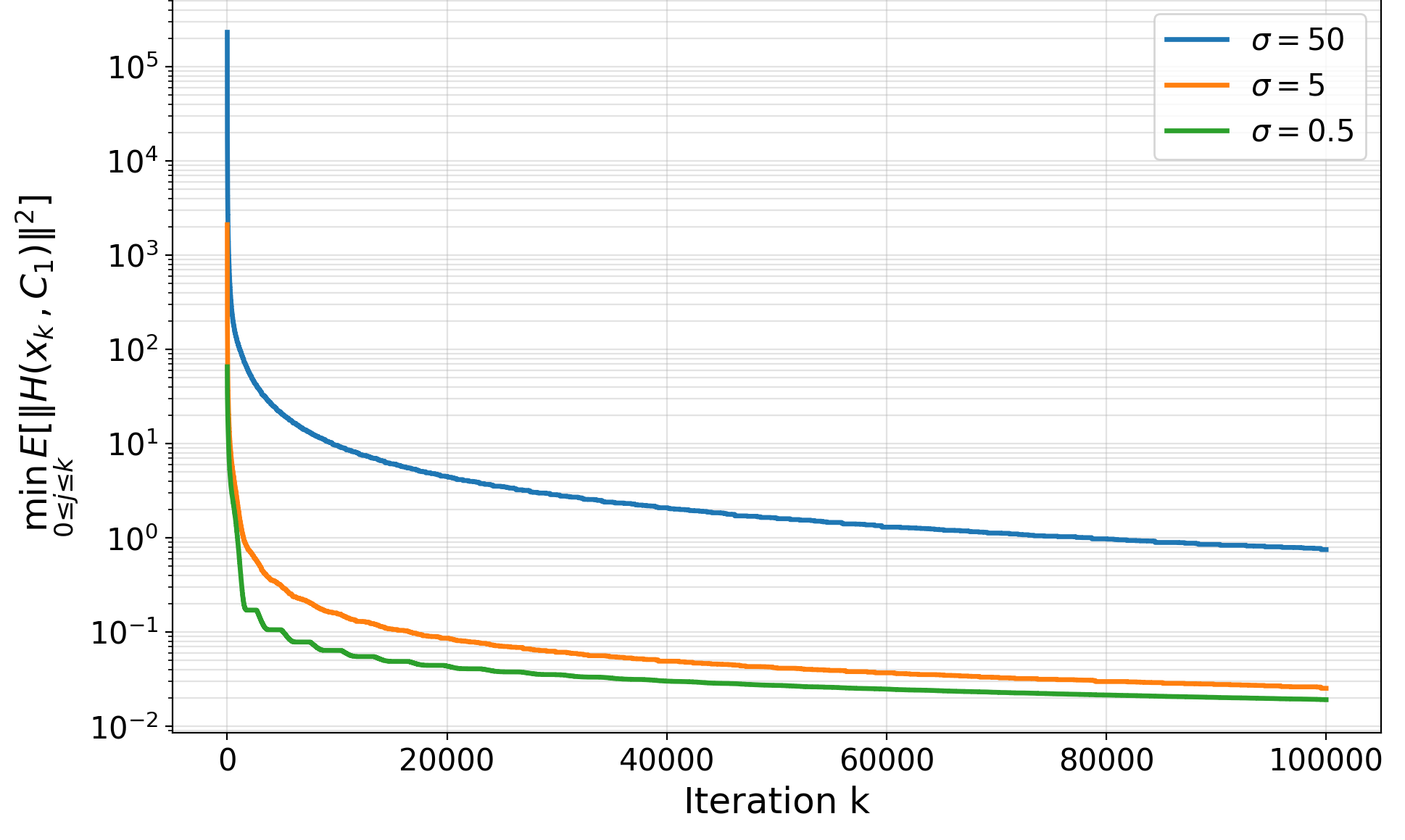
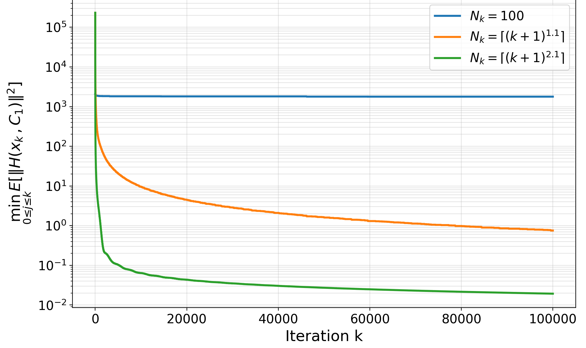
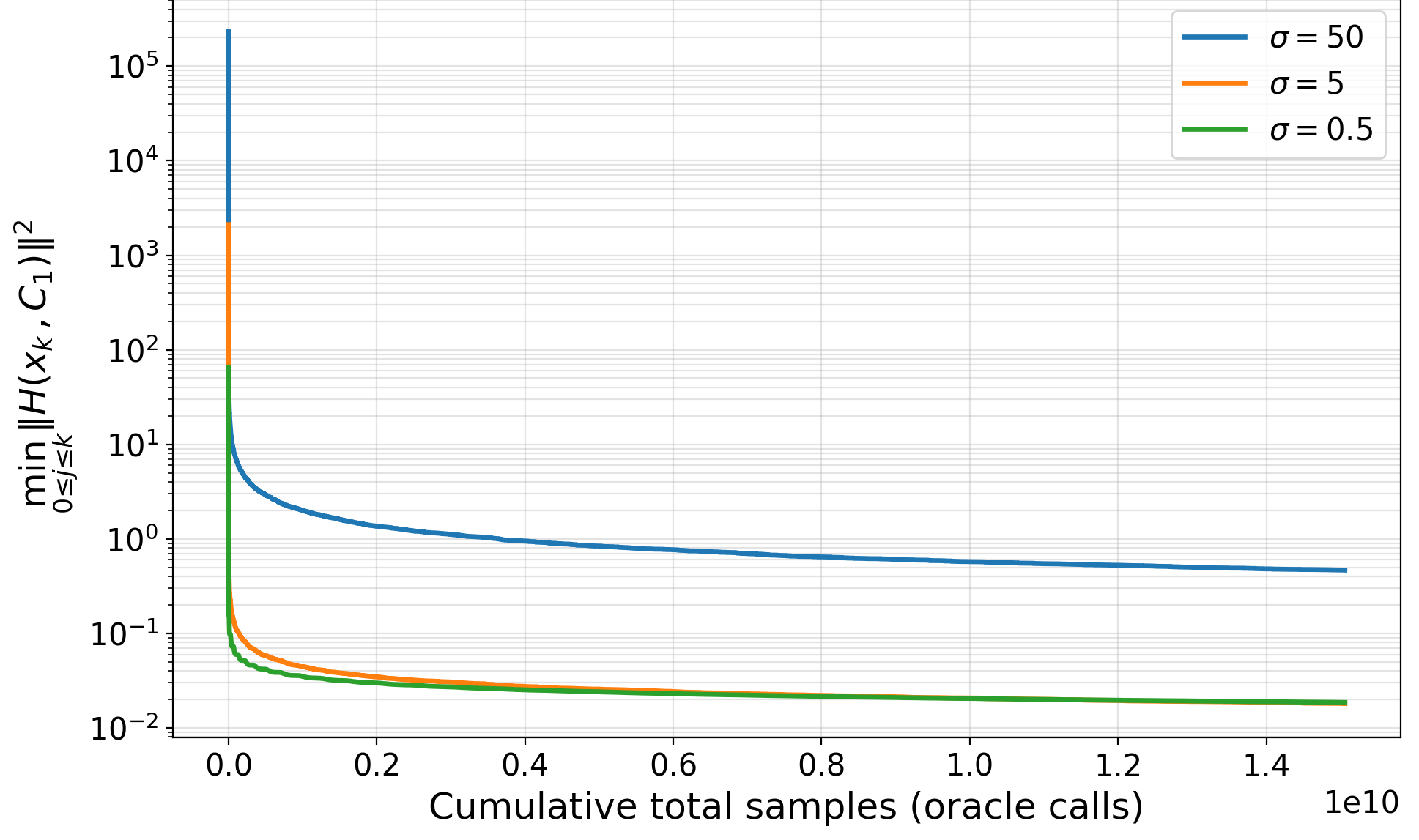
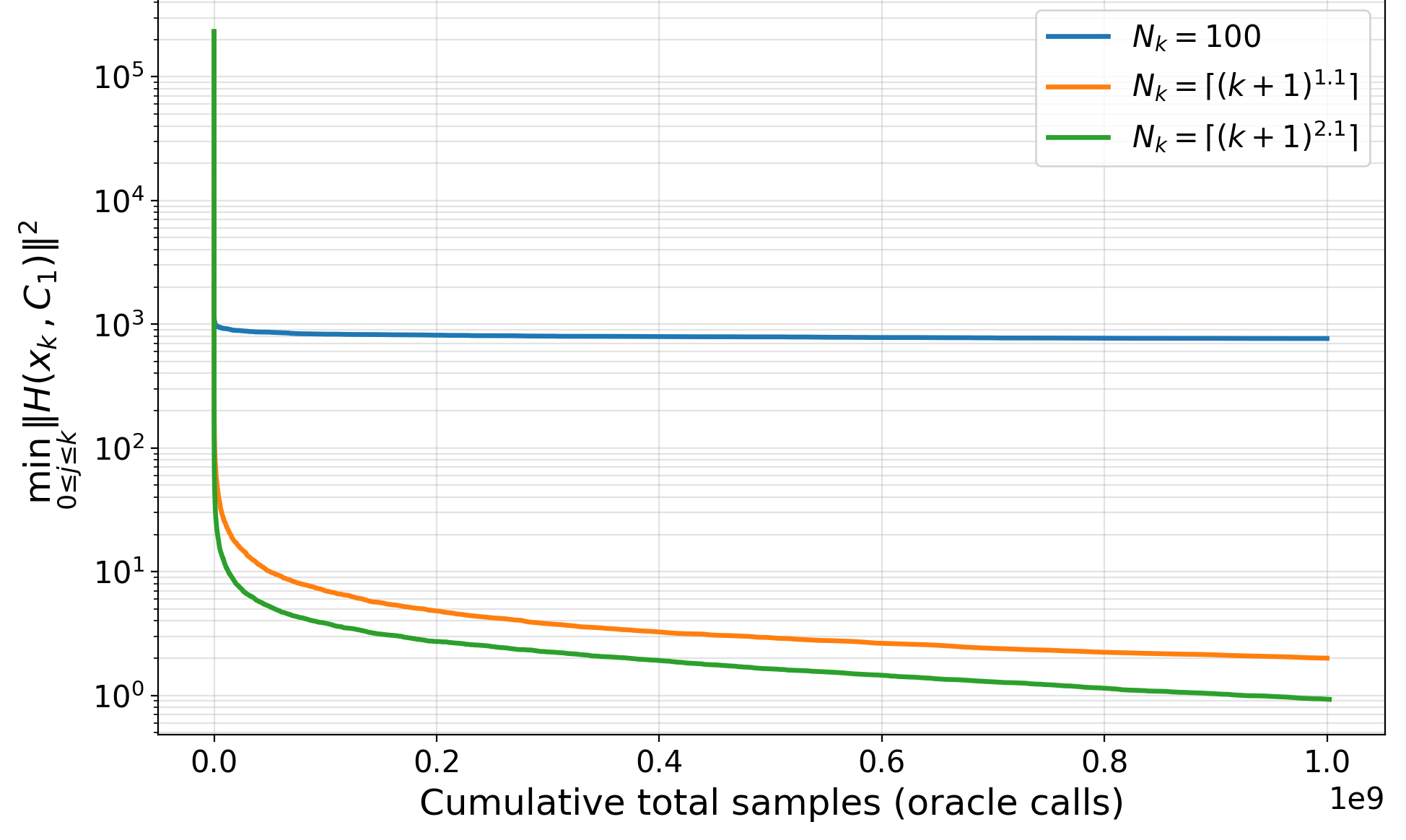
Figure 1 reports the pointwise Monte Carlo estimate of $\mathbb{E}[\|H(x_{k},\bar{\eta})\|^{2}]$. This plot illustrates the raw behavior of the residual map along the generated iterates and shows how the residual responds to different noise levels and batch-size schedules, together with $95\%$ confidence intervals. Since the theoretical result is stated for the best residual up to iteration $k$, Figure 2 reports the sample average of $\min_{0\leq j\leq k}\|H(x_{j},\bar{\eta})\|^{2}$ over the simulation runs. This quantity is the empirical counterpart of the residual controlled by our convergence-rate result. Figure 3 plots the same best residual against the cumulative number of stochastic oracle calls, highlighting the tradeoff between residual reduction and sampling effort under different batch-size choices. The constant-batch baseline illustrates that controlling the sampling error is essential in the stochastic setting, while the increasing batch-size schemes continue to reduce the best residual as the oracle budget grows. Together, these plots illustrate the behavior predicted by the theory on monotone instances that are not covered by co-coercive SIVI methods.

6 Conclusions

We studied stochastic inverse variational inequalities under monotonicity and Lipschitz continuity, without requiring co-coercivity or strong monotonicity of the mean operator. We proposed a regularized variance-controlled inverse projected-gradient method that combines Tikhonov regularization with an increasing batch-size sampling scheme. The proposed method was shown to generate almost surely bounded iterates whose distance to the SIVI solution set converges to zero almost surely. We also established an explicit $\mathcal{O}(T^{-1/2})$ nonasymptotic rate for the expected squared residual, together with the corresponding iteration and stochastic oracle complexity guarantees. A deterministic counterpart was analyzed and shown to achieve the same iteration complexity using exact operator evaluations. Numerical experiments on monotone network equilibrium problems that are not co-coercive illustrated the practical behavior of the method. Future work includes incorporating variance-reduction techniques that may improve stochastic oracle complexity, extending the framework to distributed SIVIs, and deriving sharper rates under additional structural assumptions.

References

- [1] Z. Alizadeh, A. Jalilzadeh, and F. Yousefian, Randomized Lagrangian stochastic approximation for large-scale constrained stochastic Nash games, Optimization Letters, 18 (2024), pp. 377–401.
- [2] Z. Alizadeh, F. P. Polanco, and A. Jalilzadeh, A projection-based algorithm for solving stochastic inverse variational inequality problems, in 2023 Winter Simulation Conference (WSC), IEEE, 2023, pp. 3532–3540.
- [3] Z. Alizadeh, E. Yazdandoost Hamedani, and A. Jalilzadeh, Variance-reduction for variational inequality problems with Bregman distance function, Optimization Methods and Software, (2026), pp. 1–30.
- [4] P. K. Anh and T. N. Hai, Regularized dynamics for monotone inverse variational inequalities in Hilbert spaces, Optimization and Engineering, 25 (2024), pp. 2295–2313.
- [5] J. Chen, X. Ju, E. Köbis, and Y.-C. Liou, Tikhonov type regularization methods for inverse mixed variational inequalities, Optimization, 69 (2020), pp. 401–413.
- [6] S. Dey and S. Reich, A dynamical system for solving inverse quasi-variational inequalities, Optimization, 73 (2024), pp. 1681–1701.
- [7] F. Facchinei and J.-S. Pang, Finite-dimensional Variational Inequalities and Complementarity Problems, Springer Science & Business Media, Berlin/Heidelberg, Germany, 2007.
- [8] B. He, X.-Z. He, and H. X. Liu, Solving a class of constrained ‘black-box’ inverse variational inequalities, European Journal of Operational Research, 204 (2010), pp. 391–401.
- [9] B.-S. He, A Goldstein’s type projection method for a class of variant variational inequalities, Journal of Computational Mathematics, 17 (1999), pp. 425–434.
- [10] S. He and Q.-L. Dong, An existence-uniqueness theorem and alternating contraction projection methods for inverse variational inequalities, Journal of Inequalities and Applications, 2018 (2018), pp. 1–19.
- [11] X. He and H. X. Liu, Inverse variational inequalities with projection-based solution methods, European Journal of Operational Research, 208 (2011), pp. 12–18.
- [12] A. Jalilzadeh and U. V. Shanbhag, A proximal-point algorithm with variable sample-sizes (PPAWSS) for monotone stochastic variational inequality problems, in Proceedings of the 2019 Winter Simulation Conference (WSC), N. Mustafee, K.-H. G. Bae, S. Lazarova-Molnar, M. Rabe, C. Szabo, P. Haas, and Y.-J. Son, eds., Piscataway, New Jersey, 2019, Institute of Electrical and Electronics Engineers, Inc, pp. 3551–3562.
- [13] H. Jiang and H. Xu, Stochastic approximation approaches to the stochastic variational inequality problem, Institute of Electrical and Electronics Engineers Transactions on Automatic Control, 53 (2008), pp. 1462–1475.
- [14] J. Koshal, A. Nedić, and U. V. Shanbhag, Regularized iterative stochastic approximation methods for stochastic variational inequality problems, Institute of Electrical and Electronics Engineers Transactions on Automatic Control, 58 (2012), pp. 594–609.
- [15] X.-p. Luo, Tikhonov regularization methods for inverse variational inequalities, Optimization Letters, 8 (2014), pp. 877–887.
- [16] X.-P. Luo and J. Yang, Regularization and iterative methods for monotone inverse variational inequalities, Optimization Letters, 8 (2014), pp. 1261–1272.
- [17] Y. Malitsky, Projected reflected gradient methods for monotone variational inequalities, SIAM Journal on Optimization, 25 (2015), pp. 502–520.
- [18] A. Nagurney, Network economics: A variational inequality approach, vol. 10, Springer Science & Business Media, 2013.
- [19] Y. Nesterov and L. Scrimali, Solving strongly monotone variational and quasi-variational inequalities, Discrete and Continuous Dynamical Systems, 31 (2011), pp. 1383–1396.
- [20] H. Robbins and D. Siegmund, A convergence theorem for nonnegative almost supermartingales and some applications, in Optimizing methods in statistics, Elsevier, 1971, pp. 233–257.
- [21] L. Scrimali, An inverse variational inequality approach to the evolutionary spatial price equilibrium problem, Optimization and Engineering, 13 (2012), pp. 375–387.
- [22] P. T. Vuong, X. He, and D. V. Thong, Global exponential stability of a neural network for inverse variational inequalities, Journal of Optimization Theory and Applications, 190 (2021), pp. 915–930.
- [23] H.-K. Xu, S. Dey, and V. Vetrivel, Notes on a neural network approach to inverse variational inequalities, Optimization, 70 (2021), pp. 901–910.
- [24] H. Yang and M. G. Bell, Traffic restraint, road pricing and network equilibrium, Transportation Research Part B: Methodological, 31 (1997), pp. 303–314.
- [25] F. Yousefian, A. Nedić, and U. V. Shanbhag, On smoothing, regularization, and averaging in stochastic approximation methods for stochastic variational inequality problems, Mathematical Programming, 165 (2017), pp. 391–431.
- [26] X. Zou, D. Gong, L. Wang, and Z. Chen, A novel method to solve inverse variational inequality problems based on neural networks, Neurocomputing, 173 (2016), pp. 1163–1168.