Dirichlet–Neumann waveform relaxation for heterogeneous heat equations: continuous and time discrete $L^{2}$ analysis

Abstract.

We consider two coupled linear heat equations on different spatial domains that interact through a lower dimensional interface. This models conjugate heat transfer. The problem is solved using Dirichlet–Neumann waveform relaxation. This allows us to couple separate codes for the subproblems, a so-called partitioned approach. Our overall goal is to develop more efficient partitioned methods, and to this end, we want reliable error estimates.

We use an exponentially weighted Fourier technique to derive new error estimates in $L^{2}$ for finite time $T$ in both continuous and time discrete settings. We identify an optimized relaxation parameter that guarantees superlinear convergence. Our new continuous estimate predicts linear convergence when $T$ is large, and superlinear when $T$ is small. For large $T$, our new time discrete estimate closely mirrors its continuous counterpart, whereas for small $T$, superlinear convergence in the time discrete case requires small time step $\Delta t$. We also show that convergence is fast when the contrast is large, provided that the small physical parameter domain (e.g. air) is using the Dirichlet transmission condition, and the large physical parameter domain (e.g. steel) is using the Neumann transmission condition in the Dirichlet-Neumann waveform relaxation method. Our numerical experiments confirm all these findings.

1. Introduction

Multiphysics problems involve interacting subsystems on different spatial domains, which are coupled through an interface. They are commonly modelled as coupled time-dependent partial differential equations (PDEs) that interact through a shared lower-dimensional interface [13]. Applications include fluid-structure interaction [19], heat transfer in composite materials [15], and atmosphere-ocean coupling in climate models [27]. From a computational perspective, multiphysics problems are often addressed with partitioned approaches that reuse existing single physics solvers on each subdomain. These solvers communicate only through coupling conditions, enabling independent development, maintenance, and spatial discretization [25]. Nevertheless, designing stable and efficient coupling algorithms, especially for time-dependent problems, remains challenging due to complex interface interactions.

Waveform relaxation, originally introduced in [16] for parallel simulation of large scale electronic circuits, provides a principled framework for coupling time-dependent PDEs. In waveform relaxation methods, the coupled system is solved iteratively over a time interval by alternatingly solving each subsystem and exchanging time-dependent interface data after each iteration. When combined with domain decomposition techniques, this approach leads to several algorithms, including Schwarz waveform relaxation (SWR), Dirichlet–Neumann waveform relaxation (DNWR), and Neumann-Neumann waveform relaxation (NNWR); see [8, Chapter 3] for a general overview. Applications of waveform relaxation to multiphysics problems can be found in [4, 21, 23, 25].

Achieving fast convergence in waveform relaxation methods often requires an appropriate choice of relaxation parameters. Suitable parameter choices may lead to superlinear convergence on finite time windows. This property is particularly advantageous in long time simulations. In such simulations, the global time horizon is typically decomposed into smaller time windows, and waveform relaxation iterations are performed within each time window until a stopping criterion is satisfied before marching to the next time window. Therefore, understanding how convergence depends on relaxation parameters, physical parameters, and the length of the time window, is a central topic in the analysis of waveform relaxation methods.

Several convergence analysis techniques for waveform relaxation methods have been developed in the literature [1, 4, 5, 6, 11, 17, 23]. In particular, deriving accurate error estimates is crucial as they provide practical stopping criteria. We list here some references that contain linear and superlinear error estimates. In the continuous setting, the authors in [17] derive linear $L^{2}$ error estimates for SWR applied to heterogeneous advection–diffusion equations on unbounded space-time domains, using Fourier analysis and the Plancherel theorem. In [7], the authors investigate DNWR and NNWR methods applied to homogeneous heat equations in finite time windows. Based on Laplace transform and kernel estimates, they derive superlinear $L^{\infty}$ error estimates using special relaxation parameters, $\theta=1/2$ for DNWR and $\theta=1/4$ for NNWR. In [2], we extend the analysis of DNWR applied to heterogeneous heat equations, and also derive superlinear $L^{\infty}$ error estimates for a material-dependent relaxation parameter $\theta$.

In the time discrete setting, the authors in [12] provide an analysis for the DNWR using one implicit Euler step applied to heterogeneous heat equations. They derive linear $L^{2}$ error estimates via spatial Fourier transform. An extension to multiple time steps and heterogeneous advection-diffusion equations is presented in [4], where the authors apply both implicit Euler and Runge-Kutta schemes, and derive linear $l^{2}$ error estimates using $z$-transform on unbounded space-time domains.

Despite this body of work, to our knowledge, there are no continuous and time discrete estimates for arbitrary relaxation parameters that depend on the time length $T$. Furthermore, the precise relationship between continuous superlinear convergence and its discrete counterpart, as well as the influence of the time step size and time window length, is still lacking.

The present paper closes these gaps. We consider two coupled linear heat equations with different material parameters. To analyze the convergence of DNWR applied to such problems on finite time windows, we introduce a framework based on the exponentially weighted Fourier transform proposed in [26]. Using this framework, we derive $L^{2}$ estimates for finite time lengths $T$ in both continuous and time discrete cases for arbitrary relaxation parameters $\theta$. We also show that the continuous estimate converges superlinearly for a specific choice of relaxation parameter, and compare both continuous and time discrete error estimates for this relaxation parameter. Our time discrete analysis reveals that, to preserve superlinear convergence, the time step size $\Delta t$ must be reduced as $T$ decreases. These findings further show the importance of time discrete estimates, especially when the total simulation time is split into multiple smaller time windows.

The rest of the paper is organized as follows. In Section 2, we present a convergence analysis of DNWR applied to two coupled heat equations in the continuous setting and derive superlinear error estimates using the relaxation parameter given in [2]. In Section 3, we extend our analysis to the time discrete setting using the implicit Euler scheme and derive corresponding superlinear error estimates. Section 4 compares the continuous and time discrete error estimates. Finally, in Section 5, we validate the theoretical results with numerical experiments and discuss the sharpness of our error estimates.

2. Continuous convergence analysis

We consider as our model problem two coupled linear heat equations in one dimension. Let $Q_{1}:=(-a,0)\times(0,T)$ and $Q_{2}:=(0,b)\times(0,T)$ denote two space-time domains with $a>0$, $b>0$, and the time $T>0$. In each domain $Q_{j}$, we denote by $u_{j}$ the temperature, $f_{j}$ the external force, $u_{0,j}$ the initial condition, $\alpha_{j}$ the volumetric heat capacity, and $\lambda_{i}$ the heat conductivity. For each domain, the associated heat equation reads

$$\alpha_{1}\partial_{t}u_{1}-\lambda_{1}\partial_{xx}u_{1} =f_{1} \text{in }Q_{1}, \alpha_{2}\partial_{t}u_{2}-\lambda_{2}\partial_{xx}u_{2} =f_{2} \text{in }Q_{2},$$ (1)

$$u_{1}(-a,t) =g_{l}(t) \text{in }(0,T), u_{1}(b,t) =g_{r}(t) \text{in }(0,T),$$

$$u_{1}(x,0) =u_{0,1}(x) \text{in }(-a,0), u_{2}(x,0) =u_{0,2}(x) \text{in }(0,b),$$

where $g_{l}$ and $g_{r}$ are two Dirichlet boundary conditions. These two heat equations are coupled at the interface using the two coupling conditions

$$u_{1}(0,t)=u_{2}(0,t)\ \text{ in }(0,T),\quad-\lambda_{1}\partial_{x}u_{1}(0,t)=-\lambda_{2}\partial_{x}u_{2}(0,t)\ \text{ in }(0,T).$$ (2)

The first condition imposes continuity of temperature, whereas the second ensures continuity of the heat flux at the interface.

The goal of our study is to analyze convergence of the Dirichlet–Neumann waveform relaxation (DNWR) method applied to our model problem (1)-(2). For any given initial guess $h^{0}(t)$ and the iteration index $k=1,2,\ldots$, the DNWR iteration reads

$$\alpha_{1}\partial_{t}u_{1}^{k+1}-\lambda_{1}\partial_{xx}u_{1}^{k+1} =f_{1}\ \text{ in }Q_{1}, \alpha_{2}\partial_{t}u_{2}^{k+1}-\lambda_{2}\partial_{xx}u_{2}^{k+1} =f_{2}\ \text{ in }Q_{2},$$ (DNWR)

$$u_{1}^{k+1}(-a,t) =g_{l}(t),\ -\lambda_{1}\partial_{x}u_{1}^{k+1}(0,t) =-\lambda_{2}\partial_{x}u_{2}^{k+1}(0,t),$$

$$u_{1}^{k+1}(0,t) =h^{k}(t), u_{1}^{k}(b,t) =g_{r}(t),$$

$$u_{1}^{k+1}(x,0) =u_{0,1}(x), u_{2}^{k+1}(x,0) =u_{0,2}(x),$$

and we update the Dirichlet transmission condition $h^{k}$ by

$$h^{k+1}(t):=(1-\theta)h^{k}(t)+\theta u^{k+1}_{2}(0,t),\quad\theta\in(0,1),$$

where $\theta$ is the relaxation parameter. Note that here we choose to impose the Dirichlet condition at the interface in $Q_{1}$ and the Neumann condition at the interface in $Q_{2}$.

To present our convergence analysis, we first introduce a framework based on the exponentially weighted Fourier transform proposed in [26].

Definition 1.

Let $r>0$, $\omega\in\mathbb{R}$, and $\phi$ a given function. The exponentially weighted Fourier transform of the function $\phi$ is defined by

$$\hat{\phi}(r+i\omega):=\int_{-\infty}^{\infty}\phi(t)e^{-(r+i\omega)t}\,dt,$$

if this integral is finite.

Note that the exponentially weighted Fourier transform of a function $\phi(t)$ is the standard Fourier transform applied to the function $e^{-rt}\phi(t)$, with $r>0$ the weight parameter. We use the hat notation to denote such a transform, and write the argument as $r+i\omega$ to emphasize the dependence on both the weight parameter $r$ and the frequency $\omega$. From Definition 1, we can verify that the exponentially weighted Fourier transform inherits most of the properties of the Fourier transform, such as linearity, time shifting, and differentiation. Also, it exists if $\phi\in L^{1}$. The Fourier transform of an $L^{2}$ function is in general defined via extension using the Plancherel theorem, see e.g. [10]. For the exponentially weighted Fourier transform of an $L^{2}$ function, we need additional assumptions, since the weight $e^{-rt}$ blows up as $t\to-\infty$ for $r>0$. The next result establishes the existence of this transform under an assumption that is relevant to our study.

Lemma 1.

Let $r>0$ and $\phi$ be a function defined in $(-\infty,\infty)$ such that $\left\lVert\phi\right\rVert_{L^{2}(\mathbb{R^{+}})}<\infty$ and $\phi(t)=0$ for $t<0$. Then the exponentially weighted Fourier transform of $\phi$ exists, and we have

$$\frac{1}{2\pi}\int_{-\infty}^{\infty}|\hat{\phi}(r+i\omega)|^{2}d\omega\leq\int_{-\infty}^{\infty}|\phi(t)|^{2}dt.$$

Proof.

For $r>0$ and $\phi(t)=0$ for $t<0$, we have

$$\int_{-\infty}^{\infty}\big(e^{-rt}\phi(t)\big)^{2}\,dt=\int_{0}^{\infty}\big(e^{-rt}\phi(t)\big)^{2}\,dt\leq\int_{0}^{\infty}\big(\phi(t)\big)^{2}\,dt<\infty.$$

Thus, $\psi(t):=e^{-rt}\phi(t)$ is in $L^{2}(\mathbb{R})$. Using the result in [10], the Fourier transform of $\psi$ is well defined, meaning that the exponentially weighted Fourier transform of $\phi$ is also well defined. Applying now the Plancherel theorem to $\psi$, we obtain

$$\frac{1}{2\pi}\int_{-\infty}^{\infty}|\hat{\phi}(r+i\omega)|^{2}\,d\omega=\int_{-\infty}^{\infty}\big(e^{-rt}\phi(t)\big)^{2}\,dt\leq\int_{0}^{\infty}\big(\phi(t)\big)^{2}\,dt=\int_{-\infty}^{\infty}\big(\phi(t)\big)^{2}\,dt.$$

∎

To analyze convergence, we apply the exponentially weighted Fourier transform to the error equation associated with (DNWR) and derive the contraction factor. The error equation is obtained by subtracting the solution from the model problem (1)-(2), or equivalently, by setting directly $f_{1}$, $f_{2}$, $u_{0,1}$, $u_{0,2}$, $g_{l}$, and $g_{r}$ all to zero in (DNWR). Before applying the exponentially weighted Fourier transform to (DNWR), we also need to extend the initial guess $h^{0}$ to the time interval $(-\infty,\infty)$ by setting it to zero outside its original domain. The iterates $(u_{1}^{k},u_{2}^{k},h^{k})$ for $k>0$ are then extended to $(-\infty,\infty)$ through the iteration itself. For brevity, we retain the notation $h^{0}$ and $(u_{1}^{k},u_{2}^{k},h^{k})$ for the extended functions.

For $\omega\in\mathbb{R}$ and $r\in\mathbb{R}^{+}$, the exponentially weighted Fourier transform applied to the error equation associated with (DNWR) gives

$$\alpha_{1}(r+i\omega)\hat{u}_{1}^{k+1}-\lambda_{1}\partial_{xx}\hat{u}_{1}^{k+1} =0\quad\text{ in }(-a,0),$$ (3)

$$\hat{u}_{1}^{k+1}(-a,r+i\omega) =0,$$

$$\hat{u}_{1}^{k+1}(0,r+i\omega) =\hat{h}^{k}(r+i\omega),$$

$$\alpha_{2}(r+i\omega)\hat{u}_{2}^{k+1}-\lambda_{2}\partial_{xx}\hat{u}_{2}^{k+1} =0\quad\text{ in }(0,b),$$

$$-\lambda_{1}\partial_{x}\hat{u}_{1}^{k+1}(0,r+i\omega) =-\lambda_{2}\partial_{x}\hat{u}_{2}^{k+1}(0,r+i\omega),$$

$$u_{1}^{k}(b,r+i\omega) =0,$$

$$\hat{h}^{k+1}(r+i\omega)=(1-\theta)\hat{h}^{k} (r+i\omega)+\theta\hat{u}^{k+1}_{2}(0,r+i\omega).$$

These are two coupled second-order ordinary differential equations in space, and solving them for given $\omega$ and $r$ yields the closed form solutions

$$\hat{u}_{1}^{k+1}(x,r+i\omega) =\frac{\sinh\left(\sqrt{\frac{\alpha_{1}(r+i\omega)}{\lambda_{1}}}(x+a)\right)}{\sinh\left(\sqrt{\frac{\alpha_{1}(r+i\omega)}{\lambda_{1}}}a\right)}\hat{h}^{k}(r+i\omega),$$

$$\hat{u}_{2}^{k+1}(x,r+i\omega) =\sqrt{\frac{\alpha_{1}\lambda_{1}}{\alpha_{2}\lambda_{2}}}\coth\left(\sqrt{\frac{\alpha_{1}(r+i\omega)}{\lambda_{1}}}a\right)$$

$$\times\frac{\sinh\left(\sqrt{\frac{\alpha_{2}(r+i\omega)}{\lambda_{2}}}(x-b)\right)}{\cosh\left(\sqrt{\frac{\alpha_{2}(r+i\omega)}{\lambda_{2}}}b\right)}\hat{h}^{k}(r+i\omega).$$

Using the last equation in (3), we obtain $\hat{h}^{k}(r+i\omega)=\hat{\rho}(r+i\omega)^{k}\hat{h}^{0}(r+i\omega)$, where $\hat{\rho}$ is given by

$$\hat{\rho}(s):=1-\theta-\theta\sqrt{\frac{\alpha_{1}\lambda_{1}}{\alpha_{2}\lambda_{2}}}\coth\left(\sqrt{\frac{\alpha_{1}s}{\lambda_{1}}}a\right)\tanh\left(\sqrt{\frac{\alpha_{2}s}{\lambda_{2}}}b\right),\quad s\in\mathbb{C}.$$ (4)

The function $\hat{\rho}$ evaluated at $s=r+i\omega$ with $\text{Re}(s)=r>0$ is the contraction factor associated with the transformed DNWR iteration (3). Note that $\hat{\rho}(r+i\omega)$ depends on the domain size $a$ and $b$, and the physical parameters $\alpha_{j}$ and $\lambda_{j}$, $j=1,2$. Regarding the relaxation parameter $\theta$, one wants the associated contraction factor to be small, such that  (DNWR) converges very fast. Before discussing the choice of $\theta$, we first present an error estimate for arbitrary relaxation parameter.

Theorem 1.

For any given $\theta\in(0,1)$ and $h^{0}\in L^{2}(0,T)$, the error of the iteration (DNWR) in the time interval $(0,T)$ satisfies the estimate

$$\|h^{k}\|_{L^{2}(0,T)}\leq\min_{r>0}e^{rT}\max_{\omega\in\mathbb{R}}\left|\hat{\rho}(r+i\omega)\right|^{k}\,\left\lVert h^{0}\right\rVert_{L^{2}(0,T)}.$$ (5)

Proof.

By [18, Chapter 4], $h^{k}$ exists and is well defined for $h^{0}\in L^{2}(0,T)$. For $r>0$, we have

$$\|h^{k}\|_{L^{2}(0,T)}^{2}=\int_{0}^{T}\left(h^{k}(t)\right)^{2}dt=\int_{0}^{T}e^{2rt}e^{-2rt}\left(h^{k}(t)\right)^{2} dt\leq e^{2rT}\int_{0}^{T}\left(e^{-rt}h^{k}(t)\right)^{2}dt$$

$$\leq e^{2rT}\int_{-\infty}^{\infty}\left(e^{-rt}h^{k}(t)\right)^{2}dt,$$

where in the last inequality we use the extension of $h^{k}$ to the interval $(-\infty,\infty)$. By Lemma 1, the exponentially weighted Fourier transform of $h^{k}$ exists. Applying the Plancherel theorem, we find

$$e^{2rT}\int_{-\infty}^{\infty}\left(e^{-rt}h^{k}(t)\right)^{2}dt =\frac{e^{2rT}}{2\pi}\int_{-\infty}^{\infty}\left|\hat{h}^{k}(r+i\omega)\right|^{2}d\omega$$

$$=\frac{e^{2rT}}{2\pi}\int_{-\infty}^{\infty}\left|\hat{\rho}(r+i\omega)^{k}\hat{h}^{0}(r+i\omega)\right|^{2}d\omega$$

$$\leq\frac{e^{2rT}}{2\pi}\max_{\omega\in\mathbb{R}}\left|\hat{\rho}(r+i\omega)\right|^{2k}\int_{-\infty}^{\infty}\left|\hat{h}^{0}(r+i\omega)\right|^{2}d\omega$$

$$=e^{2rT}\max_{\omega\in\mathbb{R}}\left|\hat{\rho}(r+i\omega)\right|^{2k}\int_{-\infty}^{\infty}\left|h^{0}(t)\right|^{2}dt$$

$$=e^{2rT}\max_{\omega\in\mathbb{R}}\left|\hat{\rho}(r+i\omega)\right|^{2k}\int_{0}^{T}\left|h^{0}(t)\right|^{2}dt,$$

where we use Lemma 1 once again, and the fact that $h^{0}$ is extended from $(0,T)$ to $(-\infty,\infty)$ by 0 for the last equality. Combining these computations gives

$$\|h^{k}\|_{L^{2}(0,T)}^{2}\leq e^{2rT}\max_{\omega\in\mathbb{R}}|\hat{\rho}(r+i\omega)|^{2k}\|h^{0}\|_{L^{2}(0,T)}^{2}.$$

Taking the square root on both sides and minimizing over all $r>0$ leads to (5). ∎

Theorem 1 provides a general error estimate of (DNWR) for any relaxation parameter. To achieve fast convergence, we can choose a relaxation parameter $\theta$ such that the convergence factor (4) is small. In particular, the choice

$$\theta=\frac{1}{1+\sqrt{\frac{\alpha_{1}\lambda_{1}}{\alpha_{2}\lambda_{2}}}\coth\left(\sqrt{\frac{\alpha_{1}(r+i\omega)}{\lambda_{1}}}a\right)\tanh\left(\sqrt{\frac{\alpha_{2}(r+i\omega)}{\lambda_{2}}}b\right)}$$ (6)

yields convergence in two iterations. However, this choice depends both on the weight parameter $r$ and the Fourier frequency $\omega$, making it not useful in practice. On the other hand, when the physics in both subdomains satisfy $\sqrt{\alpha_{1}/\lambda_{1}}a=\sqrt{\alpha_{2}/\lambda_{2}}b$, then the contraction factor (4) reduces to the simple form $\hat{\rho}=1-\theta-\theta\sqrt{\alpha_{1}\lambda_{1}}/\sqrt{\alpha_{2}\lambda_{2}}$, which is independent of the frequency $\omega$ and the weight parameter $r$. In this case, we obtain the optimal relaxation parameter

$$\theta^{*}:=\frac{\sqrt{\alpha_{2}\lambda_{2}}}{\sqrt{\alpha_{1}\lambda_{1}}+\sqrt{\alpha_{2}\lambda_{2}}}.$$ (7)

Note that the choice $\theta$ given in (6) converges to $\theta^{*}$ when $\omega$ goes to infinity. Therefore, for high frequencies, the DNWR iteration always converges very fast for the choice of relaxation parameter $\theta^{*}$, and thus the convergence will be independent of the mesh size, as discussed in [3, Chapter 4.7, p.174]. Furthermore, the parameter $\theta^{*}$ is much more convenient to use in practice, as it only depends on the physics of the problem. Therefore, we are interested in the impact of $\theta^{*}$ on the convergence of (DNWR) in more general cases, i.e., $\sqrt{\alpha_{1}/\lambda_{1}}a\neq\sqrt{\alpha_{2}/\lambda_{2}}b$. Substituting $\theta^{*}$ into  (4) and using properties of the differences of arguments for hyperbolic functions, we obtain

$$\hat{\rho}(s)|_{\theta^{*}}=-\frac{1}{1+\sqrt{\frac{\alpha_{2}\lambda_{2}}{\alpha_{1}\lambda_{1}}}}\frac{\sinh\left(\left(\sqrt{\frac{\alpha_{1}}{\lambda_{1}}}a-\sqrt{\frac{\alpha_{2}}{\lambda_{2}}}b\right)\sqrt{s}\right)}{\sinh\left(\sqrt{\frac{\alpha_{1}}{\lambda_{1}}}a\sqrt{s}\right)\cosh\left(\sqrt{\frac{\alpha_{2}}{\lambda_{2}}}b\sqrt{s}\right)},\quad s\in\mathbb{C}.$$ (8)

To simplify the notation, we also introduce the function

$$\hat{H}(s):=\frac{\sinh\left(|\alpha-\beta|\sqrt{s}\right)}{\sinh\left(\alpha\sqrt{s}\right)\cosh\left(\beta\sqrt{s}\right)},\quad s\in\mathbb{C}.$$ (9)

With the help of (9), the error estimate (5) associated with $\theta=\theta^{*}$ is then

$$\|h^{k}\|_{L^{2}(0,T)}\leq\left(\frac{1}{1+\sqrt{\frac{\alpha_{2}\lambda_{2}}{\alpha_{1}\lambda_{1}}}}\right)^{k}\min_{r>0}e^{rT}\max_{\omega\in\mathbb{R}}\left|\hat{H}(r+i\omega)\right|^{k}\,\left\lVert h^{0}\right\rVert_{L^{2}(0,T)},$$ (10)

where $\alpha=\sqrt{\alpha_{1}/\lambda_{1}}a$ and $\beta=\sqrt{\alpha_{2}/\lambda_{2}}b$ in $\hat{H}$ for (9). Therefore, it is sufficient to study the min-max problem associated with $\hat{H}$. We first solve the maximization problem with respect to the frequency $\omega$, then use $r$ as an auxiliary parameter to find a superlinear estimate. The next result shows the global maximum of the maximization problem.

Lemma 2.

Let $\alpha,\beta,r>0$ be given. Then the function $\hat{H}$ defined in (9) satisfies $\max_{\omega\in\mathbb{R}}|\hat{H}(r+i\omega)|=\hat{H}(r)$.

Proof.

In the proof of [20, Theorem 2], it is shown that the function $\hat{H}(s)$ with $\alpha>0$, $\beta>0$ and $\text{Re}(s)>0$, is the Laplace transform of a positive function denoted by $H(t)$. Thus, we have

$$\max_{\omega\in\mathbb{R}}|\hat{H}(r+i\omega)|=\max_{\omega\in\mathbb{R}}\Big|\int_{-\infty}^{\infty} H(t)e^{-rt-i\omega t}dt\Big|\leq\max_{\omega\in\mathbb{R}}\int_{-\infty}^{\infty}|H(t)|e^{-rt}dt$$

$$=\int_{-\infty}^{\infty}H(t)e^{-rt}dt=\hat{H}(r).$$

To see that this is actually an equality, it suffices to substitute $\omega=0$ into $\hat{H}(r+i\omega)$, which gives $\hat{H}(r)$, and thus the proof is complete. ∎

Applying Lemma 2 to (10), we have

$$\left\lVert h^{k}\right\rVert_{L^{2}(0,T)}\leq\left(\frac{1}{1+\sqrt{\frac{\alpha_{2}\lambda_{2}}{\alpha_{1}\lambda_{1}}}}\right)^{k}\min_{r>0}e^{rT}\left(\hat{H}(r)\right)^{k}\left\lVert h^{0}\right\rVert_{L^{2}(0,T)},$$ (11)

It remains to treat the minimization problem related to $r$. Depending on the physics of the problem, we have two results.

Theorem 2 (Case $\sqrt{\alpha_{1}/\lambda_{1}}a>\sqrt{\alpha_{2}/\lambda_{2}}b$).

If $\theta=\theta^{*}$ and $\sqrt{\alpha_{1}/\lambda_{1}}a>\sqrt{\alpha_{2}/\lambda_{2}}b$, then the error of the algorithm (DNWR) satisfies

$$\left\lVert h^{k}\right\rVert_{L^{2}(0,T)}\leq\left(2\frac{1-\sqrt{\frac{\alpha_{2}\lambda_{1}}{\alpha_{1}\lambda_{2}}}\frac{b}{a}}{1+\sqrt{\frac{\alpha_{2}\lambda_{2}}{\alpha_{1}\lambda_{1}}}}\right)^{k}e^{-\frac{\alpha_{2}k^{2}b^{2}}{4\lambda_{2}T}}\left\lVert h^{0}\right\rVert_{L^{2}(0,T)}.$$ (12)

Proof.

The idea is to first bound the function $\hat{H}(r)$ by an exponential function, and then to analyze the exponential function to find a minimum.

Let $0<\alpha<\beta$ and $f(x)=\beta\sinh(\alpha x)-\alpha\sinh(\beta x)$. We have $f^{\prime}(x)=\alpha\beta(\cosh(\alpha x)-\cosh(\beta x))<0$, i.e., $f$ is decreasing. Hence $f(x)\leq f(0)=0$, $\forall x>0$, yielding $\sinh(\alpha x)/\sinh(\beta x)\leq\alpha/\beta$. Taking $\alpha=\sqrt{\alpha_{1}/\lambda_{1}}a-\sqrt{\alpha_{2}/\lambda_{2}}b$, $\beta=\sqrt{\alpha_{1}/\lambda_{1}}a$ and $x=\sqrt{r}$, we find

$$\frac{\sinh\left((\sqrt{\frac{\alpha_{1}}{\lambda_{1}}}a-\sqrt{\frac{\alpha_{2}}{\lambda_{2}}}b)\sqrt{r}\right)}{\sinh\left(\sqrt{\frac{\alpha_{1}}{\lambda_{1}}}a\sqrt{r}\right)}\leq\frac{\sqrt{\frac{\alpha_{1}}{\lambda_{1}}}a-\sqrt{\frac{\alpha_{2}}{\lambda_{2}}}b}{\sqrt{\frac{\alpha_{1}}{\lambda_{1}}}a}=1-\sqrt{\frac{\alpha_{2}\lambda_{1}}{\alpha_{1}\lambda_{2}}}\frac{b}{a}.$$ (13)

On the other hand, using the definition of the hyperbolic cosine, we have

$$\frac{1}{\cosh\left(\sqrt{\frac{\alpha_{2}}{\lambda_{2}}}b\sqrt{r}\right)}=\frac{2\exp\left(-\sqrt{\frac{\alpha_{2}}{\lambda_{2}}}b\sqrt{r}\right)}{1+\exp\left(-2\sqrt{\frac{\alpha_{2}}{\lambda_{2}}}b\sqrt{r}\right)}\leq 2\exp\left(-\sqrt{\frac{\alpha_{2}}{\lambda_{2}}}b\sqrt{r}\right).$$ (14)

The product of (13) and (14) to the power $k$ gives

$$\left(\frac{\sinh\left(\left(\sqrt{\frac{\alpha_{1}}{\lambda_{1}}}a-\sqrt{\frac{\alpha_{2}}{\lambda_{2}}}b\right)\sqrt{r}\right)}{\sinh\left(\sqrt{\frac{\alpha_{1}}{\lambda_{1}}}a\sqrt{r}\right)\cosh\left(\sqrt{\frac{\alpha_{2}}{\lambda_{2}}}b\sqrt{r}\right)}\right)^{k}\leq 2^{k}\left(1-\sqrt{\frac{\alpha_{2}\lambda_{1}}{\alpha_{1}\lambda_{2}}}\frac{b}{a}\right)^{k}\exp\left(-kb\sqrt{\frac{\alpha_{2}r}{\lambda_{2}}}\right).$$ (15)

Therefore, the estimate (11) with the definition (9) of $\hat{H}$ becomes

$$\left\lVert h^{k}\right\rVert_{L^{2}(0,T)}\leq \left(\frac{1}{1+\sqrt{\frac{\alpha_{2}\lambda_{2}}{\alpha_{1}\lambda_{1}}}}\right)^{k}\min_{r>0}e^{rT}\left(\hat{H}(r)\right)^{k}\left\lVert h^{0}\right\rVert_{L^{2}(0,T)}$$ (16)

$$\leq \left(2\frac{1-\sqrt{\frac{\alpha_{2}\lambda_{1}}{\alpha_{1}\lambda_{2}}}\frac{b}{a}}{1+\sqrt{\frac{\alpha_{2}\lambda_{2}}{\alpha_{1}\lambda_{1}}}}\right)^{k}\min_{r>0}e^{rT-kb\sqrt{\frac{\alpha_{2}r}{\lambda_{2}}}}\left\lVert h^{0}\right\rVert_{L^{2}(0,T)}.$$

It remains now to find the minimum of $\exp(rT-kb\sqrt{\alpha_{2}r}/\sqrt{\lambda_{2}})$. Differentiating it with respect to $r$ gives $(T-kb\sqrt{\alpha_{2}}/\sqrt{4\lambda_{2}r})\exp(rT-kb\sqrt{\alpha_{2}r}/\sqrt{\lambda_{2}})$. Setting the derivative to 0 yields the extremal point

$$r^{*}_{1c}=\frac{\alpha_{2}k^{2}b^{2}}{4\lambda_{2}T^{2}}.$$ (17)

Note that the derivative changes sign from negative to positive at $r^{*}_{1c}$, and thus $r^{*}_{1c}$ is a minimum. Substituting $r^{*}_{1c}$ into the second inequality in (16) gives the estimate (12). ∎

Theorem 3 (Case $\sqrt{\alpha_{1}/\lambda_{1}}a<\sqrt{\alpha_{2}/\lambda_{2}}b$).

Let $\theta=\theta^{*}$. If $\sqrt{\alpha_{1}/\lambda_{1}}a<\sqrt{\alpha_{2}/\lambda_{2}}b<2\sqrt{\alpha_{1}/\lambda_{1}}a$, then the error of the algorithm (DNWR) satisfies

$$\left\lVert h^{k}\right\rVert_{L^{2}(0,T)}\leq\left(2\frac{\sqrt{\frac{\alpha_{2}\lambda_{1}}{\alpha_{1}\lambda_{2}}}\frac{b}{a}-1}{\sqrt{\frac{\alpha_{2}\lambda_{2}}{\alpha_{1}\lambda_{1}}}+1}\right)^{k}e^{-\frac{\alpha_{2}k^{2}b^{2}}{4\lambda_{2}T}}\left\lVert h^{0}\right\rVert_{L^{2}(0,T)}.$$ (18)

If $\sqrt{\alpha_{2}/\lambda_{2}}b\geq 2\sqrt{\alpha_{1}/\lambda_{1}}a$, then the error of the algorithm (DNWR) satisfies

$$\left\lVert h^{k}\right\rVert_{L^{2}(0,T)}\leq\left(2\frac{\sqrt{\frac{\alpha_{2}\lambda_{1}}{\alpha_{1}\lambda_{2}}}\frac{b}{a}-1}{\sqrt{\frac{\alpha_{2}\lambda_{2}}{\alpha_{1}\lambda_{1}}}+1}\right)^{k}e^{-\frac{\alpha_{1}k^{2}a^{2}}{\lambda_{1}T}}\left\lVert h^{0}\right\rVert_{L^{2}(0,T)}.$$ (19)

Proof.

The idea is the same as in the proof of Theorem 2. If $\sqrt{\alpha_{1}/\lambda_{1}}a<\sqrt{\alpha_{2}/\lambda_{2}}b<2\sqrt{\alpha_{1}/\lambda_{1}}a$, then $0<\sqrt{\alpha_{2}/\lambda_{2}}b-\sqrt{\alpha_{1}/\lambda_{1}}a<\sqrt{\alpha_{1}/\lambda_{1}}a$. We can thus follow the same steps as in the proof of Theorem 2 by taking $\alpha=\sqrt{\alpha_{2}/\lambda_{2}}b-\sqrt{\alpha_{1}/\lambda_{1}}a$ and $\beta=\sqrt{\alpha_{1}/\lambda_{1}}a$. We find a similar bound as (15), namely

$$\left(\frac{\sinh\left(\left(\sqrt{\frac{\alpha_{2}}{\lambda_{2}}}b-\sqrt{\frac{\alpha_{1}}{\lambda_{1}}}a\right)\sqrt{r}\right)}{\sinh\left(\sqrt{\frac{\alpha_{1}}{\lambda_{1}}}a\sqrt{r}\right)\cosh\left(\sqrt{\frac{\alpha_{2}}{\lambda_{2}}}b\sqrt{r}\right)}\right)^{k}\leq 2^{k}\left(\sqrt{\frac{\alpha_{2}\lambda_{1}}{\alpha_{1}\lambda_{2}}}\frac{b}{a}-1\right)^{k}\exp\left(-kb\sqrt{\frac{\alpha_{2}r}{\lambda_{2}}}\right).$$ (20)

This leads to the same miminizer $r^{*}_{1c}$ given in (17), and we obtain the estimate (18).

If $\sqrt{\alpha_{2}/\lambda_{2}}b\geq 2\sqrt{\alpha_{1}/\lambda_{1}}a$, we substitute $\tau=\exp(-2\sqrt{r})$ and obtain

$$\frac{\sinh\left(\left(\sqrt{\frac{\alpha_{2}}{\lambda_{2}}}b-\sqrt{\frac{\alpha_{1}}{\lambda_{1}}}a\right)\sqrt{r}\right)}{\sinh\left(\sqrt{\frac{\alpha_{1}}{\lambda_{1}}}a\sqrt{r}\right)\cosh\left(\sqrt{\frac{\alpha_{2}}{\lambda_{2}}}b\sqrt{r}\right)}=2\tau^{\sqrt{\frac{\alpha_{1}}{\lambda_{1}}}a}\frac{1-\tau^{\sqrt{\frac{\alpha_{2}}{\lambda_{2}}}b-\sqrt{\frac{\alpha_{1}}{\lambda_{1}}}a}}{\left(1+\tau^{\sqrt{\frac{\alpha_{2}}{\lambda_{2}}}b}\right)\left(1-\tau^{\sqrt{\frac{\alpha_{1}}{\lambda_{1}}}a}\right)}.$$

The latter fraction can be bounded by

$$\frac{1-\tau^{\sqrt{\frac{\alpha_{2}}{\lambda_{2}}}b-\sqrt{\frac{\alpha_{1}}{\lambda_{1}}}a}}{\left(1+\tau^{\sqrt{\frac{\alpha_{2}}{\lambda_{2}}}b}\right)\left(1-\tau^{\sqrt{\frac{\alpha_{1}}{\lambda_{1}}}a}\right)}\leq\frac{1-\tau^{\sqrt{\frac{\alpha_{2}}{\lambda_{2}}}b-\sqrt{\frac{\alpha_{1}}{\lambda_{1}}}a}}{1-\tau^{\sqrt{\frac{\alpha_{1}}{\lambda_{1}}}a}}.$$

Let now $\alpha\geq\beta>0$ and $f(x)=\beta(1-e^{-\alpha x})-\alpha(1-e^{-\beta x})$, then $f^{\prime}(x)=\alpha\beta(e^{-\alpha x}-e^{-\beta x})\leq 0$, i.e., $f$ is non-increasing. Hence, $f(x)\leq f(0)=0$, $\forall x>0$, yielding $(1-e^{-\alpha x})/((1-e^{-\beta x}))\leq\alpha/\beta$. Taking then $\alpha=\sqrt{\alpha_{2}/\lambda_{2}}b-\sqrt{\alpha_{1}/\lambda_{1}}a$, $\beta=\sqrt{\alpha_{1}/\lambda_{1}}a$ and $x=2\sqrt{r}$ gives

$$\frac{1-\tau^{\sqrt{\frac{\alpha_{2}}{\lambda_{2}}}b-\sqrt{\frac{\alpha_{1}}{\lambda_{1}}}a}}{1-\tau^{\sqrt{\frac{\alpha_{1}}{\lambda_{1}}}a}}\leq\frac{\sqrt{\frac{\alpha_{2}}{\lambda_{2}}}b-\sqrt{\frac{\alpha_{1}}{\lambda_{1}}}a}{\sqrt{\frac{\alpha_{1}}{\lambda_{1}}}a}=\sqrt{\frac{\alpha_{2}\lambda_{1}}{\alpha_{1}\lambda_{2}}}\frac{b}{a}-1.$$ (21)

This implies that

$$\left(\frac{\sinh\left(\left(\sqrt{\frac{\alpha_{2}}{\lambda_{2}}}b-\sqrt{\frac{\alpha_{1}}{\lambda_{1}}}a\right)\sqrt{r}\right)}{\sinh\left(\sqrt{\frac{\alpha_{1}}{\lambda_{1}}}a\sqrt{r}\right)\cosh\left(\sqrt{\frac{\alpha_{2}}{\lambda_{2}}}b\sqrt{r}\right)}\right)^{k}\leq 2^{k}\left(\sqrt{\frac{\alpha_{2}\lambda_{1}}{\alpha_{1}\lambda_{2}}}\frac{b}{a}-1\right)^{k}\exp\left(-2k\sqrt{\frac{\alpha_{1}r}{\lambda_{1}}}a\right).$$ (22)

Note that the exponential part is slightly different compared with (20) in the previous case. Using the bound (22), our estimate (11) in this case becomes

$$\left\lVert h^{k}\right\rVert_{L^{2}(0,T)}\leq \left(\frac{1}{1+\sqrt{\frac{\alpha_{2}\lambda_{2}}{\alpha_{1}\lambda_{1}}}}\right)^{k}\min_{r>0}e^{rT}\left(\hat{H}(r)\right)^{k}\left\lVert h^{0}\right\rVert_{L^{2}(0,T)}$$ (23)

$$\leq \left(2\frac{\sqrt{\frac{\alpha_{2}\lambda_{1}}{\alpha_{1}\lambda_{2}}}\frac{b}{a}-1}{\sqrt{\frac{\alpha_{2}\lambda_{2}}{\alpha_{1}\lambda_{1}}}+1}\right)^{k}\min_{r>0}e^{rT-2ka\sqrt{\frac{\alpha_{1}r}{\lambda_{1}}}}\left\lVert h^{0}\right\rVert_{L^{2}(0,T)}.$$

Once again, we take the derivative with respect to $r$ of the function $\exp(rT-2ka\sqrt{\alpha_{1}r}/\sqrt{\lambda_{1}})$ to find the minimum

$$r^{*}_{2c}=\frac{\alpha_{1}k^{2}a^{2}}{\lambda_{1}T^{2}}.$$ (24)

Substituting $r^{*}_{2c}$ back into the second inequality of (23) gives the estimate (19). ∎

For $\theta=\theta^{*}$, the error estimates given in Theorems 2 and 3 contain both linear and superlinear behavior. When the time $T$ is large, the exponential part in (12), (18), (19) is close to one, and the estimates predict linear convergence. In contrast, the exponential part plays an important role when the time $T$ is small, and we obtain superlinear convergence. Furthermore, the weight parameters (17) and (24) depend on the subdomain size and physical parameters: $r^{*}_{1c}$ depends on those in $Q_{2}$ and $r^{*}_{2c}$ depends on those in $Q_{1}$.

On the other hand, the weight parameter $r$ is an auxiliary parameter that is only used in our analysis to derive error estimates. As shown in the proofs of Theorems 2 and 3, our approach to treat the minimization problem (11) is as follows: we first bound $\hat{H}(r)$ by a function of $r$, and then solve the resulting minimization problem to obtain $r^{*}_{1c}$ and $r^{*}_{2c}$, instead of solving (11) directly. We can then substitute $r^{*}_{1c}$ and $r^{*}_{2c}$ into the function $\hat{H}(r)$ in (11) to obtain sharper error estimates.

Corollary 1.

For $\theta=\theta^{*}$, the error of the algorithm (DNWR) satisfies

$$\left\lVert h^{k}\right\rVert_{L^{2}(0,T)}\leq\left(\frac{\hat{H}(r^{*})}{1+\sqrt{\frac{\alpha_{2}\lambda_{2}}{\alpha_{1}\lambda_{1}}}}\right)^{k}e^{r^{*}T}\left\lVert h^{0}\right\rVert_{L^{2}(0,T)},$$ (25)

where $r^{*}$ denotes $r_{1c}^{*}$ or $r_{2c}^{*}$ depending on the value of $\sqrt{\alpha_{1}/\lambda_{1}}a$ and $\sqrt{\alpha_{2}/\lambda_{2}}b$.

Although the error estimate (25) is sharper than those in Theorems 2 and 3, it is less straightforward to see the linear and superlinear convergence behavior in (25), as the dependence on $T$ is hidden in the value of $r^{*}$.

In general, one splits a long simulation time into smaller time windows, performs waveform relaxation methods within each window until a stopping criterion is satisfied, and then moves to the next one. Therefore, we are interested in the values of $T$ that lead to superlinear convergence. The error estimates provided in Theorems 2 and 3 indicate how one should choose the time window length, which will be further discussed in Section 4.

3. Time discrete analysis

The error estimates obtained in the continuous setting do not clarify the influence of the time step size. In this section, we provide a detailed time discrete analysis of (DNWR). We discretize the time interval $[0,T]$ with $0=t_{0}<t_{1}<\ldots<t_{N}=T$, where $t_{n}=n\Delta t$ and $\Delta t=T/N$. We denote by $u^{n}$ the approximation of the solution $u$ at the time $t_{n}$ and $\boldsymbol{u}=(u^{1},\ldots,u^{N})^{\top}$. As before, we use $k$ to denote the index of the waveform iteration. The implicit Euler method applied to (DNWR) reads: For $n=0,\ldots,N-1$,

$$\frac{\alpha_{1}}{\Delta t}(u_{1}^{n+1,k+1}-u_{1}^{n,k+1})-\lambda_{1}\partial_{xx}u_{1}^{n+1,k+1} =f_{1}^{n+1}\ \text{ in }\ (-a,0),$$ (DNWR-IE)

$$u_{1}^{n+1,k+1}(-a)=g_{l}^{n+1},\quad u_{1}^{n+1,k+1}(0) =h^{n+1,k},$$

$$u_{1}^{0,k+1}(x) =u_{0,1}(x)$$

$$\frac{\alpha_{2}}{\Delta t}(u_{2}^{n+1,k+1}-u_{2}^{n,k+1})-\lambda_{2}\partial_{xx}u_{2}^{n+1,k+1} =f_{2}^{n+1}\ \text{ in }\ (0,b),$$

$$u_{2}^{n+1,k+1}(b)=g_{r}^{n+1},\quad-\lambda_{1}\partial_{x}u_{1}^{n+1,k+1}(0) =-\lambda_{2}\partial_{x}u_{2}^{n+1,k+1}(0),$$

$$u_{2}^{0,k+1}(x) =u_{0,2}(x),$$

$$h^{n+1,k+1}=(1-\theta)h^{n+1,k}+\theta u^{n+1,k+1}_{2}(0),\quad\theta\in(0,1).$$

To remain in a similar analysis framework as in Section 2, we keep using the exponentially weighted technique. In the continuous case, we use the Fourier transform; correspondingly, we consider here the discrete-time Fourier transform, which possesses properties, such as linearity, time shifting, differentiation, and the Parseval Theorem. We refer to the monograph [24, Chapter 2.9] for a detailed introduction. To take advantage of the Parseval Theorem, we define the exponentially weighted discrete-time Fourier transform as follows.

Definition 2.

Let $r>0$, $\Delta t>0$, $\omega\in[-\pi,\pi]$, and $\{\phi^{n}\}_{n\in\mathbb{Z}}$ be a given sequence. The exponentially weighted discrete-time Fourier transform of $\{\phi^{n}\}_{n\in\mathbb{Z}}$ is defined by

$$\widehat{\phi}(r\Delta t+i\omega):=\sum_{n\in\mathbb{Z}}\phi^{n}e^{-n(r\Delta t+i\omega)},$$

if this series is finite.

We use the notation wide hat here to denote the exponentially weighted discrete-time Fourier transform to distinguish it from the exponentially weighted Fourier transform in the continuous case. In addition, similar to Definition 1, we write the argument as $r\Delta t+i\omega$ to emphasize the dependence on the weight parameter $r$, the time step size $\Delta t$ and the frequency $\omega$. In general, the weight $e^{-rn\Delta t}$ blows up as $n\to-\infty$ for $r>0$. The next Lemma provides a similar result to Lemma 1.

Lemma 3.

Let $r>0$ and $\boldsymbol{\phi}=\{\phi^{n}\}_{n\in\mathbb{Z}}$ be a sequence such that $\sum_{n\in\mathbb{N}}(\phi^{n})^{2}<\infty$, and $\phi^{n}=0$ for $n<0$. Then the exponentially weighted discrete-time Fourier transform exists, and we have

$$\frac{1}{2\pi}\int_{-\pi}^{\pi}|\widehat{\phi}(r\Delta t+i\omega)|^{2}d\omega\leq\left\lVert\boldsymbol{\phi}\right\rVert_{l^{2}}^{2}.$$

Proof.

For $r>0$ and $\Delta t>0$, $e^{-r\Delta t}<1$. We then have $\sum_{n\in\mathbb{Z}}(e^{-r\Delta t}\phi^{n})^{2}\leq\sum_{n\in\mathbb{Z}}(\phi^{n})^{2}<\infty$. The time-discrete Fourier transform of the sequence $e^{-r\Delta t}\boldsymbol{\phi}$ therefore exists. Applying Parseval’s theorem to $e^{-r\Delta t}\boldsymbol{\phi}$, we find

$$\frac{1}{2\pi}\int_{-\pi}^{\pi}\left|\widehat{\phi}(r\Delta t+i\omega)\right|^{2}d\omega=\sum_{n\in\mathbb{Z}}(e^{-r\Delta tn}\phi^{n})^{2}\leq\sum_{n\in\mathbb{Z}}(\phi^{n})^{2}=\left\lVert\boldsymbol{\phi}\right\rVert_{l^{2}}^{2}.$$

∎

To analyze convergence in the time discrete case, we focus on the error equation associated with (DNWR-IE), which consists of setting $f_{1}^{n},f_{2}^{n},g_{l}^{n},g_{r}^{n},u_{0,1},u_{0,2}$ all to zero in (DNWR-IE). We also extend the initial guess $\{h^{n,0}\}_{n=0}^{N}$ by 0 to $\boldsymbol{h}^{0}:=\{h^{n,0}\}_{n\in\mathbb{Z}}$. The iterates $\{u_{1}^{n,k},u_{2}^{n,k},h^{n,k}\}_{n=0}^{N}$ for $k>0$ are then extended for $n\in\mathbb{Z}$ through the iteration itself. For brevity, we retain the notation $h^{n,0}$ and $u_{1}^{n,k},u_{2}^{n,k},h^{n,k}$ for the extended version. The exponentially weighted discrete-time Fourier transform applied to the error equations gives

$$\frac{\alpha_{1}}{\Delta t}(e^{r\Delta t+i\omega}\widehat{u}^{k+1}_{1}-\widehat{u}^{k+1}_{1})-\lambda_{1}\partial_{xx}e^{r\Delta t+i\omega}\widehat{u}^{k+1}_{1} =0,$$ (26)

$$\widehat{u}^{k+1}_{1}(-a)=0,\quad\widehat{u}^{k+1}_{1}(0) =\widehat{h}^{k},$$

$$\frac{\alpha_{2}}{\Delta t}(e^{r\Delta t+i\omega}\widehat{u}_{2}^{k+1}-\widehat{u}_{2}^{k+1})-\lambda_{2}\partial_{xx}e^{r\Delta t+i\omega}\widehat{u}_{2}^{k+1} =0,$$

$$\widehat{u}^{k+1}_{2}(b)=0,\quad-\lambda_{1}\partial_{x}\widehat{u}^{k+1}_{1}(0) =-\lambda_{2}\partial_{x}\widehat{u}^{k+1}_{2}(0),$$

$$\widehat{h}^{k+1}=(1-\theta)\,\widehat{h}^{k}+ \theta\,\widehat{u}^{k+1}_{2}(0).$$

Similar to (3), these are two coupled second-order ordinary differential equations in space, and solving them separately yields the closed form solutions

$$\widehat{u}_{1}^{k}(x) =\frac{\sinh\left((x+a)\sqrt{\frac{\alpha_{1}(1-e^{-r\Delta t-i\omega})}{\lambda_{1}\Delta t}}\right)}{\sinh\left(a\sqrt{\frac{\alpha_{1}(1-e^{-r\Delta t-i\omega})}{\lambda_{1}\Delta t}}\right)}\widehat{h}^{k},$$

$$\widehat{u}_{2}^{k}(x) =\sqrt{\frac{\alpha_{1}\lambda_{1}}{\alpha_{2}\lambda_{2}}}\frac{\cosh\left(a\sqrt{\frac{\alpha_{1}(1-e^{-r\Delta t-i\omega})}{\lambda_{1}\Delta t}}\right)}{\sinh\left(a\sqrt{\frac{\alpha_{1}(1-e^{-r\Delta t-i\omega})}{\lambda_{1}\Delta t}}\right)}\frac{\sinh\left((x-b)\sqrt{\frac{\alpha_{2}(1-e^{-r\Delta t-i\omega})}{\lambda_{2}\Delta t}}\right)}{\cosh\left(b\sqrt{\frac{\alpha_{2}(1-e^{-r\Delta t-i\omega})}{\lambda_{2}\Delta t}}\right)}\widehat{h}^{k}.$$

Using the last equation in (26), we obtain by induction that

$$\widehat{h}^{k}=\hat{\rho}\left(\frac{1-e^{-r\Delta t-i\omega}}{\Delta t}\right)^{k}\widehat{h}^{0},$$

where the function $\hat{\rho}$ is defined in (4). Similar to the continuous case, the convergence factor $\hat{\rho}((1-e^{-r\Delta t-i\omega})/\Delta t)$ depends on the subdomain sizes and the physical parameters that are all hidden in the function $\hat{\rho}$. Besides, the convergence factor also depends on the time step size $\Delta t$. Our goal is to understand how the choice of time step size influences the convergence behavior, and the relationship between the continuous and time discrete analysis. As in Theorem 1, we first present an error estimate of the time discrete iteration (DNWR-IE) for arbitrary relaxation parameter $\theta\in(0,1)$.

Theorem 4.

For any given $\theta\in(0,1)$, the error of the time discrete iteration (DNWR-IE) satisfies the estimate

$$\|\boldsymbol{h}^{k}\|_{l^{2}}\leq\min_{r>0}e^{rT}\max_{\omega\in[-\pi,\pi]}\left|\hat{\rho}\left(\frac{1-e^{-r\Delta t-i\omega}}{\Delta t}\right)^{k}\right|\|\boldsymbol{h}^{0}\|_{l^{2}},$$ (27)

where $\hat{\rho}$ is defined in (4).

Proof.

As $r>0$, we have

$$\|\boldsymbol{h}^{k}\|_{l^{2}}^{2}=\sum_{n=0}^{N}e^{2r\Delta tn}e^{-2r\Delta tn}\left(h^{n,k}\right)^{2} \leq e^{2rT}\sum_{n=0}^{N}\left(e^{-r\Delta tn}h^{n,k}\right)^{2}$$

$$\leq e^{2rT}\sum_{n\in\mathbb{Z}}\left(e^{-r\Delta tn}h^{n,k}\right)^{2},$$

where in the last inequality we use the extension of the sequence $\boldsymbol{h}^{k}$. By Lemma 3, the exponentially weighted discrete-time Fourier transform of $\boldsymbol{h}^{k}$ exists. Applying the Parseval theorem yields

$$e^{2rT}\sum_{n\in\mathbb{Z}}\left(e^{-r\Delta tn}h^{n,k}\right)^{2} =\frac{e^{2rT}}{2\pi}\int_{-\pi}^{\pi}\left|\widehat{h}^{k}(r\Delta t+i\omega)\right|^{2}d\omega$$

$$=\frac{e^{2rT}}{2\pi}\int_{-\pi}^{\pi}\left|\hat{\rho}\left(\frac{1-e^{-r\Delta t-i\omega}}{\Delta t}\right)^{k}\widehat{h}^{0}(r\Delta t+i\omega)\right|^{2}d\omega$$

$$\leq\frac{e^{2rT}}{2\pi}\max_{\omega\in[-\pi,\pi]}\left|\hat{\rho}\left(\frac{1-e^{-r\Delta t-i\omega}}{\Delta t}\right)\right|^{2k}\int_{-\pi}^{\pi}\left|\widehat{h}^{0}(r\Delta t+i\omega)\right|^{2}d\omega$$

$$\leq e^{2rT}\max_{\omega\in[-\pi,\pi]}\left|\hat{\rho}\left(\frac{1-e^{-r\Delta t-i\omega}}{\Delta t}\right)\right|^{2k}\|\boldsymbol{h}^{0}\|_{l^{2}}^{2},$$

where we use Lemma 3 for the last inequality. Combining these computations gives

$$\|\boldsymbol{h}^{k}\|_{l^{2}}^{2}\leq e^{2rT}\max_{\omega\in[-\pi,\pi]}\left|\hat{\rho}\left(\frac{1-e^{-r\Delta t-i\omega}}{\Delta t}\right)\right|^{2k}\|\boldsymbol{h}^{0}\|_{l^{2}}^{2}.$$

Taking the square root on both sides and minimizing over all $r>0$ leads to (27). ∎

This estimate involves a min-max problem which is generally difficult to analyze. However, analogous to the continuous case, when the physical parameters in both subdomains satisfy $\sqrt{\alpha_{1}/\lambda_{1}}a=\sqrt{\alpha_{2}/\lambda_{2}}b$, the optimal relaxation parameter $\theta^{*}$ given in (7) again ensures convergence in two iterations for the time discrete iteration. Furthermore, we have obtained superlinear convergence in the continuous analysis using such $\theta^{*}$ for more general physical conditions, i.e., $\sqrt{\alpha_{1}/\lambda_{1}}a\neq\sqrt{\alpha_{2}/\lambda_{2}}b$. We are interested in the convergence behavior of the time discrete iteration (DNWR-IE) for this special choice of relaxation parameter $\theta^{*}$ and the dependence on the time step size $\Delta t$. As in the continuous case, with the help of (8) and (9), we can rewrite the error estimate (27) for $\theta=\theta^{*}$ as

$$\|\boldsymbol{h}^{k}\|_{l^{2}}\leq\left(\frac{1}{1+\sqrt{\frac{\alpha_{2}\lambda_{2}}{\alpha_{1}\lambda_{1}}}}\right)^{k}\min_{r>0}e^{rT}\max_{\omega\in[-\pi,\pi]}\left|\hat{H}\left(\frac{1-e^{-r\Delta t-i\omega}}{\Delta t}\right)^{k}\right|\|\boldsymbol{h}^{0}\|_{l^{2}},$$ (28)

where $\alpha=\sqrt{\alpha_{1}/\lambda_{1}}a$ and $\beta=\sqrt{\alpha_{2}/\lambda_{2}}b$ in the function $\hat{H}$ defined in (9). Therefore, when $\theta=\theta^{*}$, it suffices to study the min-max problem associated with $\hat{H}$. We start by giving a similar result to Lemma 2 for the global maximum of the maximization problem.

Lemma 4.

Let $\alpha>0$, $\beta>0$, $r>0$, and $\Delta t>0$, then the function $\hat{H}$ defined in (9) satisfies

$$\max_{\omega\in[-\pi,\pi]}\left|\hat{H}\left(\frac{1-e^{-r\Delta t-i\omega}}{\Delta t}\right)\right|=\hat{H}\left(\frac{1-e^{-r\Delta t}}{\Delta t}\right).$$

Proof.

Let $g(\omega)=(1-e^{-r\Delta t-i\omega})/\Delta t$. For $r>0$ and $\Delta t>0$, the image of $g$ is a subset of a shifted half-plane, or more precisely

$$\text{Image}(g)=\left\{g(\omega):\,\omega\in[-\pi,\pi]\right\}\subset\left\{g(0)+x+iy\,:\,x\geq 0,y\in\mathbb{R}\right\}=:S.$$

Thus, we can transfer the maximization problem to the set $S$ as

$$\max_{\omega\in[-\pi,\pi]}\left|\hat{H}\left(g(\omega)\right)\right|\leq\max_{(x,y)\in S}\left|\hat{H}\left(g(0)+x+iy\right)\right|=\max_{x\geq 0}\left|\hat{H}\left(g(0)+x\right)\right|,$$

where Lemma 2 was used in the last equality. We now show that $\hat{H}$ is nonincreasing as a function of a real variable. Let $\gamma$ be a real number. Depending on the value of $\alpha$ and $\beta$, we have three cases.

1. If $\alpha=\beta$, $\hat{H}=0$.

2. If $\alpha>\beta>0$, we have

   $$\hat{H}^{\prime}(\gamma)=\frac{\alpha\sinh(2\beta\gamma)-\beta\sinh(2\alpha\gamma)}{2\sinh^{2}(\alpha\gamma)\cosh^{2}(\beta\gamma)}<0,$$

   since $\alpha\sinh(2\beta\gamma)<\beta\sinh(2\alpha\gamma)$. In fact, the function $f(\gamma):=\alpha\sinh(2\beta\gamma)-\beta\sinh(2\alpha\gamma)$ satisfies

   $$f(0)=0,\quad f^{\prime}(\gamma)=2\alpha\beta(\cosh(2\beta\gamma)-\cosh(2\alpha\gamma))<0,$$

   for $\alpha>\beta>0$.

3. If $\beta>\alpha>0$, we have

   $$\hat{H}^{\prime}(\gamma)=\frac{\beta\sinh(2\alpha\gamma)-\alpha\sinh(2\beta\gamma)}{2\sinh^{2}(a\gamma)\cosh^{2}(b\gamma)}<0,$$

   following a similar reasoning as in (ii).

Therefore, we have

$$\hat{H}\left(g(0)+x\right)\leq\hat{H}\left(g(0)\right),\quad\forall x\geq 0.$$

This implies that

$$\max_{\omega\in[-\pi,\pi]}\left|\hat{H}\left(g(\omega)\right)\right|\leq\hat{H}\left(g(0)\right)=\hat{H}\left(\frac{1-e^{-r\Delta t}}{\Delta t}\right).$$

∎

Applying Lemma 4 to (28), we have

$$\|\boldsymbol{h}^{k}\|_{l^{2}}\leq\left(\frac{1}{1+\sqrt{\frac{\alpha_{2}\lambda_{2}}{\alpha_{1}\lambda_{1}}}}\right)^{k}\min_{r>0}e^{rT}\hat{H}\left(\frac{1-e^{-r\Delta t}}{\Delta t}\right)^{k}\|\boldsymbol{h}^{0}\|_{l^{2}}.$$ (29)

As in the continuous case, we address the minimization problem for $r$ according to the underlying physics of the problem.

Theorem 5 (Case $\sqrt{\alpha_{1}/\lambda_{1}}a>\sqrt{\alpha_{2}/\lambda_{2}}b$).

If $\theta=\theta^{*}$ and $\sqrt{\alpha_{1}/\lambda_{1}}a>\sqrt{\alpha_{2}/\lambda_{2}}b$, then the error of the time discrete iterates (DNWR-IE) satisfies

$$\|\boldsymbol{h}^{k}\|_{l^{2}}\leq\left(2\frac{1-\sqrt{\frac{\alpha_{2}\lambda_{1}}{\alpha_{1}\lambda_{2}}}\frac{b}{a}}{1+\sqrt{\frac{\alpha_{2}\lambda_{2}}{\alpha_{1}\lambda_{1}}}}\right)^{k}\phi_{1}(r_{1d}^{*})\left\lVert\boldsymbol{h}^{0}\right\rVert_{l^{2}},$$ (30)

with

$$\phi_{1}(r)=\exp\left(rT-kb\sqrt{\frac{\alpha_{2}}{\lambda_{2}}}\sqrt{\frac{1-e^{-r\Delta t}}{\Delta t}}\right),\ r^{*}_{1d}=\frac{1}{\Delta t}\log\left(\frac{1+\sqrt{\frac{\alpha_{2}\Delta t}{\lambda_{2}T^{2}}b^{2}k^{2}+1}}{2}\right).$$ (31)

Proof.

Reusing the bound (15) given in the proof of Theorem 2 with $r=(1-\exp(-r\Delta t))/\Delta t$ yields

$$\left(\frac{1}{1+\sqrt{\frac{\alpha_{2}\lambda_{2}}{\alpha_{1}\lambda_{1}}}}\right)^{k}\min_{r>0}e^{rT}\hat{H}\left(\frac{1-e^{-r\Delta t}}{\Delta t}\right)^{k}\leq\left(2\frac{\bigl|1-\sqrt{\frac{\alpha_{2}\lambda_{1}}{\alpha_{1}\lambda_{2}}}\frac{b}{a}\bigr|}{1+\sqrt{\frac{\alpha_{2}\lambda_{2}}{\alpha_{1}\lambda_{1}}}}\right)^{k}\min_{r>0}\phi_{1}(r).$$ (32)

Differentiating $\phi_{1}$ yields

$$\phi_{1}^{\prime}(r)=\left(T-\frac{kb}{2}\sqrt{\frac{\alpha_{2}}{\lambda_{2}}}\sqrt{\frac{\Delta t}{1-e^{-r\Delta t}}}e^{-r\Delta t}\right)\exp\left(rT-kb\sqrt{\frac{\alpha_{2}}{\lambda_{2}}}\sqrt{\frac{1-e^{-r\Delta t}}{\Delta t}}\right).$$

Setting the latter to 0 yields the extremal point $r^{*}_{1d}$ given in (31). The derivative $\phi_{1}^{\prime}(r)$ is negative for $r<r^{*}_{1d}$ and positive for $r>r^{*}_{1d}$, since $e^{-r\Delta t}\sqrt{\Delta t/(1-e^{-r\Delta t})}$ is a decreasing function of $r$. This implies that the extremum is indeed a minimum. Inserting $r^{*}_{1d}$ into $\phi_{1}$ in (32) gives the estimate (30). ∎

Theorem 6 (Case $\sqrt{\alpha_{1}/\lambda_{1}}a<\sqrt{\alpha_{2}/\lambda_{2}}b$).

Let $\theta=\theta^{*}$. If $\sqrt{\alpha_{1}/\lambda_{1}}a<\sqrt{\alpha_{2}/\lambda_{2}}b<2\sqrt{\alpha_{1}/\lambda_{1}}a$, then the error of the iterates (DNWR-IE) satisfies

$$\|\boldsymbol{h}^{k}\|_{l^{2}}\leq\left(2\frac{\sqrt{\frac{\alpha_{2}\lambda_{1}}{\alpha_{1}\lambda_{2}}}\frac{b}{a}-1}{\sqrt{\frac{\alpha_{2}\lambda_{2}}{\alpha_{1}\lambda_{1}}}+1}\right)^{k}\phi_{1}(r^{*}_{1d})\|\boldsymbol{h}^{0}\|_{l^{2}},$$ (33)

with $r^{*}_{1d}$ and $\phi_{1}$ defined in (31).

If $\sqrt{\alpha_{2}/\lambda_{2}}b\geq 2\sqrt{\alpha_{1}/\lambda_{1}}a$, then the error of the iterates (DNWR-IE) satisfies

$$\|\boldsymbol{h}^{k}\|_{l^{2}}\leq\left(2\frac{\sqrt{\frac{\alpha_{2}\lambda_{1}}{\alpha_{1}\lambda_{2}}}\frac{b}{a}-1}{\sqrt{\frac{\alpha_{2}\lambda_{2}}{\alpha_{1}\lambda_{1}}}+1}\right)^{k}\phi_{2}(r_{2d}^{*})\|\boldsymbol{h}^{0}\|_{l^{2}},$$ (34)

with

$$\phi_{2}(r)=\exp\left(rT-ka\sqrt{\frac{\alpha_{1}}{\lambda_{1}}}\sqrt{\frac{1-e^{-r\Delta t}}{\Delta t}}\right),\ r^{*}_{2d}=\frac{1}{\Delta t}\log\left(\frac{1+\sqrt{4\frac{\alpha_{1}\Delta t}{\lambda_{1}T^{2}}a^{2}k^{2}+1}}{2}\right).$$ (35)

Proof.

The proof for the case $\sqrt{\alpha_{1}/\lambda_{1}}a<\sqrt{\alpha_{2}/\lambda_{2}}b<2\sqrt{\alpha_{1}/\lambda_{1}}a$ follows the same steps as that of Theorem 5, except we make use of the bound (20). This leads to the same optimized $r^{*}_{1d}$ given in (31).

For $\sqrt{\alpha_{2}/\lambda_{2}}b\geq 2\sqrt{\alpha_{1}/\lambda_{1}}a$, we follow once again the proof of Theorem 5, but use instead the bound (21), which gives

$$\left(\frac{1}{1+\sqrt{\frac{\alpha_{2}\lambda_{2}}{\alpha_{1}\lambda_{1}}}}\right)^{k}\min_{r>0}e^{rT}\hat{H}\left(\frac{1-e^{-r\Delta t}}{\Delta t}\right)^{k}\leq\left(2\frac{\frac{\sqrt{\alpha_{2}\lambda_{1}}b}{\sqrt{\alpha_{1}\lambda_{2}}a}-1}{\sqrt{\frac{\alpha_{2}\lambda_{2}}{\alpha_{1}\lambda_{1}}}+1}\right)^{k}\min_{r>0}\phi_{2}(r).$$

Setting then $\phi^{\prime}_{2}(r)=0$, we obtain the optimum value of $r^{*}_{2d}$ (35). Inserting it into $\phi_{2}$ gives the result (34). ∎

Theorems 5 and 6 provide time discrete error estimates that depend on both time $T$ and step size $\Delta t$. Note that $\phi_{1}(r^{*}_{1d})$ and $\phi_{2}(r^{*}_{2d})$ are guaranteed to be less than or equal to 1, since $\phi_{1}$ and $\phi_{2}$ are continuous for $r>0$ and $1=\phi_{1}(0)\geq\min_{r>0}\phi_{1}(r)=\phi_{1}(r^{*}_{1d})$ and $1=\phi_{2}(0)\geq\min_{r>0}\phi_{2}(r)=\phi_{2}(r^{*}_{2d})$. Thus, the exponential factor is guaranteed to be nonincreasing.

Furthermore, the time discrete estimates share the same linear factor as in the continuous estimates given in Theorems 2 and 3. Similarly to the continuous case, the weights (31) and (35) depend on the subdomain size and physical parameters. As they are auxiliary parameters that are only used in our analysis to derive error estimates, we can also substitute them directly into (11) to obtain sharper error estimates, as in Corollary 1.

Corollary 2.

For $\theta=\theta^{*}$, the error of the iterates (DNWR-IE) satisfies

$$\|\boldsymbol{h}^{k}\|_{l^{2}}\leq\left(\frac{\hat{H}\left(\frac{1-e^{-r^{*}\Delta t}}{\Delta t}\right)}{1+\sqrt{\frac{\alpha_{2}\lambda_{2}}{\alpha_{1}\lambda_{1}}}}\right)^{k}e^{r^{*}T}\|\boldsymbol{h}^{0}\|_{l^{2}},$$ (36)

where $r^{*}$ denotes $r_{1d^{*}}$ or $r_{2d^{*}}$ depending on the value of $\sqrt{\alpha_{1}/\lambda_{1}}a$ and $\sqrt{\alpha_{2}/\lambda_{2}}b$.

Once again, the error estimate (36) is sharper than those in Theorems 5 and 6, since we directly inject the value $r^{*}$ (i.e., $r_{1d}^{*}$ or $r_{2d}^{*}$) into the function $\hat{H}$ instead of bounding it first. However, its dependence on the time step size $\Delta t$ is hidden in the value of $r^{*}$. To compare with the estimates obtained in the continuous case and to understand the impact of $\Delta t$, we still need to use the estimates derived in Theorems 5 and 6.

4. Comparison of continuous and time discrete estimates

Before comparing our continuous and time discrete error estimates, we first discuss the relation of the convergence factors. Recall the function $\hat{\rho}$ defined in (4). In the continuous case, the convergence factor is $\hat{\rho}(r+i\omega)$ with $r>0$ and $\omega\in\mathbb{R}$, while in the time discrete case, it is $\hat{\rho}((1-\exp(r\Delta t+i\omega))/\Delta t)$ with $r>0$, $\Delta t>0$, and $\omega\in[-\pi,\pi]$. We have

$$\lim_{\Delta t\rightarrow 0}\frac{1-\exp(r\Delta t+i\omega)}{\Delta t}=\lim_{\Delta t\rightarrow 0}\frac{1-\exp(\Delta t(r+i\frac{\omega}{\Delta t}))}{\Delta t}=r+i\frac{\omega}{\Delta t}.$$

The time discrete frequency $\omega/\Delta t$ is in $[-\pi/\Delta t,\pi/\Delta t]$, which goes to $\mathbb{R}$ as $\Delta t$ goes to 0, thus the time discrete convergence factor approaches the continuous one.

For $\theta=\theta^{*}$ defined in (7), the convergence factor can be simplified using $\hat{H}$ defined in (9). By Lemmas 2 and 4, the maximum of $\hat{H}$ in the two cases are $\hat{H}(r)$ and $\hat{H}((1-e^{-r\Delta t})/\Delta t)$. As shown in the proof of Lemma 4, $\hat{H}$ is nonincreasing for real values, and we always have $(1-e^{-r\Delta t})/\Delta t\leq r$. This implies that

$$\hat{H}\left(\frac{1-e^{-r\Delta t}}{\Delta t}\right)\geq\hat{H}(r),$$

and thus the time discrete error estimate (29) is larger than (11).

Now we compare the time discrete estimates obtained in Theorems 5, 6 and Corollary 2 with their continuous counterparts Theorems 2, 3 and Corollary 1. We focus on the optimal $r^{*}$ for small and large $T$ and $\Delta t$. As shown in Theorems 2, 3, 5 and 6, the optimal $r^{*}$ is obtained based on the choice of the material parameters and domain sizes. In the case $\sqrt{\alpha_{1}/\lambda_{1}}a>\sqrt{\alpha_{2}/\lambda_{2}}b$, the optimal $r^{*}$ are $r^{*}_{1c}$ (17) and $r^{*}_{1d}$ (31). Taylor expanding $r^{*}_{1d}$ in $(\alpha_{2}\Delta t)/(\lambda_{2}T^{2})b^{2}k^{2}$ gives

$$r^{*}_{1d}=\frac{1}{\Delta t}\log\left(\frac{1+\sqrt{\frac{\alpha_{2}\Delta t}{\lambda_{2}T^{2}}b^{2}k^{2}+1}}{2}\right)=\underbrace{\frac{\alpha_{2}b^{2}k^{2}}{4\lambda_{2}T^{2}}}_{=r^{*}_{1c}}+O\left(\Delta t\left(\frac{\alpha_{2}b^{2}k^{2}}{\lambda_{2}T^{2}}\right)^{2}\right).$$ (37)

Thus, $r^{*}_{1d}$ is close to $r^{*}_{1c}$ if $\Delta t\left(\alpha_{2}b^{2}k^{2}/(\lambda_{2}T^{2})\right)^{2}$ is small. Note that the material parameters and the domain size affect the latter term in the same way as $r^{*}_{1c}$. This acts as a scaling determining which $\Delta t$ and $T$ are considered small or large.

For large $T$, $(\alpha_{2}\Delta t)/(\lambda_{2}T^{2})b^{2}k^{2}$ is small even for large $\Delta t$. Thus, $r^{*}_{1d}\approx r^{*}_{1c}$ independently of $\Delta t$. In addition, $r^{*}_{1c}\approx 0$ for large $T$, implying linear convergence in (12), and similarly for $r^{*}_{1d}$ in (30). Note that the linear convergence factor is the same in both the time discrete and continuous estimates. Therefore, for large $T$, both estimates predict linear convergence. The convergence factor is guaranteed to be small when $\lambda_{1}/\lambda_{2}$ is small. This was also observed in a fully discrete analysis in [23].

For small $T$, the continuous estimate (12) shows superlinear convergence. If $\Delta t$ is also small with respect to $T$, then $r_{1d}^{*}$ is still close to $r_{1c}^{*}$, which leads to superlinear convergence in the time discrete estimate (30). On the other hand, if $\Delta t$ is not small enough, then $(\alpha_{2}\Delta t)/(\lambda_{2}T^{2})b^{2}k^{2}$ can become large, implying that the continuous and time discrete error estimates behave qualitatively different.

Similar results are obtained by Taylor expanding $r^{*}_{2d}$ in $(\alpha_{1}\Delta t)/(\lambda_{1}T^{2})a^{2}k^{2}$ and comparing with $r^{*}_{2c}$.

These theoretical results are illustrated by the following two numerical test cases:

• Case A: a low contrast test case with physical material parameters $\alpha_{1}=4$, $\alpha_{2}=\lambda_{1}=\lambda_{2}=1$.

• Case B: a more realistic high contrast case with physical material parameters for air $\alpha=1299$ and $\lambda=0.0243$, and for steel $\alpha=3.47\times 10^{6}$ and $\lambda=48.9$. The air and steel domains can be arranged either as air-steel or steel-air, depending on whether the Dirichlet condition is imposed on the air or the steel domain.

For all our tests, we use the relaxation parameter $\theta^{*}$ defined in (7) and consider $a=b=1$, i.e., the space domain $(-1,1)$. We solve the minimization problems given in (11) and (29) numerically, using the Nelder-Mead optimization algorithm in SciPy with an absolute tolerance of $10^{-6}$. The code for these tests can be found in the GitHub repository [14].

In Case A, the physical parameters satisfy the condition $\sqrt{\alpha_{1}/\lambda_{1}}a=2>1=\sqrt{\alpha_{2}/\lambda_{2}}b$. Thus, we compare the estimates in (11), (12) and (25) for the continuous case, and (29), (30) and (36) for the time discrete case. We set $T=1/4$ and $\Delta t=1/64$ and illustrate these estimates as a function of the iteration number $k$ in Figure 1.

Figure 1. The continuous and time-discrete explicit error estimates as well as the improved version for Case A with $\Delta t=1/64$ and $T=1/4$. As a baseline this plot also includes numerically calculated error estimates from Theorem 1 and 4.

We observe that the time discrete error estimate is indeed larger than the continuous estimate in Figure 1.

For both continuous and time discrete error bounds (12) and (30) shown in green and red curves, we observe superlinear behavior as expected, since the time $T$ is small. However, they are both less accurate compared to (11) and (29). To improve it, we use the error bounds in (25) and (36) shown in purple and brown curves. The latter two are much sharper in both cases compared with (12) and (30). Thus, both (25) and (36) can provide more accurate predictions of the convergence behavior with the help of the auxiliary parameter $r^{*}$. Similar results are obtained also for other physical parameters using $r^{*}_{2c}$ and $r^{*}_{2d}$. In the following experiments, we will use (25) and (36).

Next, we focus on the qualitative impact of the time $T$ and the time step $\Delta t$ on the error estimates (25) and (36). To illustrate the dependence on $T$ and $\Delta t$, we show both continuous and time discrete estimates in Figure 2.

Figure 2. Continuous and time discrete error estimates for Case A with different $\Delta t$ and $T$. Left: $T=1/4$. Middle: $T=1$. Right: $T=4$.

We observe once again that the time discrete estimate is always larger than the continuous one. When the time step $\Delta t$ is reduced, the time discrete estimate approaches the continuous estimate. The choice of $\Delta t$ plays an important role when $T$ is small and the continuous estimate predicts superlinear convergence, here $T=1/4$. A sufficiently small $\Delta t$ is required for the time discrete estimate to capture the same superlinear convergence behavior. Furthermore, both time discrete and continuous error estimates are nearly identical when $T$ is large (in our case $T=1$), and we only observe linear convergence behavior. This is expected since the linear convergence part is the same for both continuous and time discrete error estimates.

To illustrate the impact of the material parameters, we also show both continuous and time discrete estimates for Case B in Figure 3.

Figure 3. Continuous and time discrete error estimates for Case B with different $\Delta t$ and $T$. Left: $T=5\times 10^{3}$. Middle: $T=5\times 10^{4}$. Right: $T=5\times 10^{5}$. Top: steel-air. Bottom: air-steel.

The steel-air configuration, i.e., steel on the left domain with Dirichlet transmission condition and air on the right domain with Neumann transmission condition, exhibits a similar behavior as in Case A. To see the same convergence behavior as in Case A, both $T$ and $\Delta t$ are required to be much larger for the steel-air configuration.

The air-steel configuration exhibits very fast linear convergence, reaching the error $10^{-12}$ in less than 3 iterations for all tested $T$ and $\Delta t$. Furthermore, both continuous and time discrete estimates are very close, implying that the choice of $\Delta t$ has less impact on the convergence for the air-steel configuration. This is expected since the linear part in the error estimates is the same for both continuous and time discrete cases, which does not depend on the time step $\Delta t$.

Note that the ratio $\alpha/\lambda$ is much larger in Case B (order of 10⁴) than in Case A (order of 1). Thus, one needs to increase $T$ or decrease $\Delta t$ in Case B to keep the factor $\Delta t\left(\alpha_{2}b^{2}k^{2}/(\lambda_{2}T^{2})\right)^{2}$ in (37) small to see a similar difference between the continuous and time discrete estimates as in Case A, as shown in Figure 2 and the first row of Figure 3.

Overall, for large values of $T$, both continuous and time discrete estimates exhibit linear convergence, and the choice of $\Delta t$ has little impact on the observed convergence behavior. In contrast, for small $T$, the continuous estimate shows superlinear convergence, and the choice of $\Delta t$ plays a significant role in the resulting convergence behavior. To preserve the superlinear convergence for the time discrete estimate, $\Delta t$ needs to be small with respect to $T$. For small $T$ and large $\Delta t$, our experiments show that the time discrete estimate converges linearly, with the convergence factor decreasing as $\Delta t$ decreases.

5. Numerical experiments

We now compare the continuous (25) and time discrete estimates (36) with the observed convergence behavior of DNWR iterations applied to two coupled linear heat equations with different material parameters. We set the relaxation parameter $\theta=\theta^{*}$ defined in (7). We first study a one dimensional case corresponding to the problem described in (DNWR) and then extend our study to a two dimensional case.

5.1. One dimensional experiment

We use the implicit Euler method to discretize the time domain and the centered finite difference method to discretize the space domain. We consider a very fine spatial mesh size $\Delta x=10^{-4}$ to ensure that the effect of the time discretization dominates over the spatial discretization. The initial waveform error $\boldsymbol{h}^{0}=\{h^{n,0}\}_{n=0}^{N}$ is set to be random, as discussed in [9, Section 5.1]. The Python code for these experiments is based on [22] and can be found in the GitHub repository [14]. Figure 4 shows the error of the first and the third iteration for Case A with $T=2$ and $\Delta t=1/64$.

Figure 4. Error of the DNWR iterations for Case A with $T=2$ and $\Delta t=1/64$. Left: First iteration. Right: Third iteration.

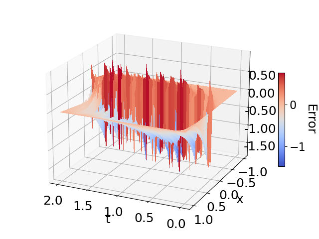
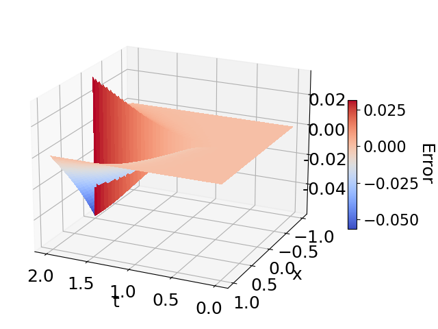
On the left of Figure 4, the waveform error $\boldsymbol{h}^{0}$ after the first iteration is mainly centered around the interface $x=0$ with nonsmooth information. The error is decreased by a factor of $100$ after the third iteration and becomes very smooth. In addition, it increases in $t$ and attains its maximum at $T=2$. This is expected, as the error estimates in both continuous and time discrete cases are increasing with respect to $T$.

We then compare the observed convergence behavior with both continuous and time discrete estimates in Figure 5 for Case A.

Figure 5. Comparison of continuous error estimate (blue), time discrete error estimates (orange) and normalized error $\|\boldsymbol{h}^{k}|_{l^{2}}/\|\boldsymbol{h}^{0}|_{l^{2}}$ of DNWR iterations (green) for Case A. Top: $T=1/4$. Bottom $T=1$. Left: $\Delta t=1/16$. Middle: $\Delta t=1/64$. Right: $\Delta t=1/256$.

In this test, we consider two times $T=1/4$ and $T=1$, and three time steps $\Delta t=1/16,1/64,1/256$. We observe that the time discrete estimate accurately captures the convergence behavior of the DNWR iterations for all cases, and the method converges more slowly than predicted by the continuous estimate, when $\Delta t$ is large, and the numerical solutions are not accurate. For small $\Delta t$, when the resulting numerical solutions become more accurate and close to the true solutions, convergence becomes as fast as predicted by the continuous estimate. As discussed in Section 4, we see that the time discrete error estimate approaches the continuous one when $\Delta t\to 0$. Comparing the top and bottom row in Figure 5, we also see that the continuous estimate becomes more accurate when $\Delta t$ is kept fixed and $T$ increases, which confirms our analysis in Section 4.

We next use the high contrast steel-air Case B to illustrate that one has to assign the Dirichlet and Neumann conditions accordingly to get fast convergence. Figure 6 shows the result for $T=5\times 10^{4}$, at the top the air-steel case, and at the bottom the steel-air case. To illustrate the behaviour for small and large time steps, we use $\Delta t=10,10^{4}$, based on the time discrete and the continuous estimate being close and far apart for these values, respectively, in Figure 3.

Figure 6. Comparison of continuous error estimate (blue), time discrete error estimates (orange) and normalized error $\|\boldsymbol{h}^{k}\|_{l^{2}}/\|\boldsymbol{h}^{0}\|_{l^{2}}$ of (DNWR) iterations (green) for Case B with $T=5\times 10^{4}$. Left: $\Delta t=10^{4}$. Right: $\Delta t=10$. Top: air-steel. Bottom: steel-air.

We see that convergence for the air-steel case is much faster than the steel-air case, and both the continuous and time discrete estimates predict this well. In the much slower steel-air case, the behavior is similar to Figure 5.

5.2. Two dimensional experiment

We now consider a higher dimensional air and steel example to show that our DNWR method can also be highly effective in higher dimensions, and the good assignment of the Dirichlet and Neumann conditions for fast convergence still holds. We consider $\Omega_{1}=(-1,0)\times(0,1)$, $\Omega_{2}=(-1,0)\times(0,1)$, $Q_{1}=\Omega_{1}\times(0,T)$, and $Q_{2}=\Omega_{2}\times(0,T)$. Let $\Gamma=\{0\}\times(0,1)\times(0,T)$ denote the interface between the two domains. The error equations of the corresponding DNWR iterations are given by

$$\alpha_{1}\partial_{t}u_{1}^{k+1}-\lambda_{1}\left(\partial_{xx}u_{1}^{k+1}+\partial_{yy}u_{1}^{k+1}\right) =0\ \text{ in }Q_{1},$$ (38)

$$u_{1}^{k+1}(0,y,t) =h^{k}(y,t)\ \text{ in }(0,1)\times(0,T),$$

$$u_{1}^{k}(x,y,t) =0\ \text{ on }\partial\Omega_{1}\setminus\Gamma,$$

$$u_{1}^{k+1}(x,y,0) =0\ \text{ in }\Omega_{1},$$

$$\alpha_{2}\partial_{t}u_{2}^{k+1}-\lambda_{2}\left(\partial_{xx}u_{2}^{k+1}+\partial_{yy}u_{2}^{k+1}\right) =0\ \text{ in }Q_{2},$$

$$-\lambda_{1}\partial_{x}u_{1}^{k+1}(0,y,t) =-\lambda_{2}\partial_{x}u_{2}^{k+1}(0,y,t)\ \text{ in }(0,1)\times(0,T),$$

$$u_{2}^{k+1}(x,y,t) =0\ \text{ on }\partial\Omega_{2}\setminus\Gamma,$$

$$u_{2}^{k+1}(x,y,0) =0\ \text{ in }\Omega_{2},$$

$$h^{k+1}(y,t)=(1-\theta)h^{k}(y,t)+\theta u_{2}^{k+1}(0, y,t)\ \text{ in }(0,1)\times(0,T).$$

To solve (38), we discretize the problem using the implicit Euler method in time and a linear finite element method in space. The Python code is available in the GitHub repository [22]. Similar to the 1D case, the initial waveform error $\boldsymbol{h}^{0}$ is chosen randomly.

In Figure 7, we show at the top the air-steel case, and at the bottom the steel-air case for $T=5\times 10^{4}$, the spatial mesh size $\Delta x=\Delta y=10^{-3}$. To see an effect of the time discretization in this experiment, we set $\Delta t=10^{4},5\times 10^{3}$.

Figure 7. Illustration of normalized error $\|\boldsymbol{h}^{k}\|_{l^{2}}/\|\boldsymbol{h}^{0}\|_{l^{2}}$ of 2D DNWR iterations using Case B with $T=5\times 10^{4}$ and $\Delta x=\Delta y=10^{-3}$. Left: $\Delta t=10^{4}$. Right: $\Delta t=5\times 10^{3}$. Top: air-steel. Bottom: steel-air.

We observe once again that convergence for the air-steel case is much faster than the steel-air case, and our 1D estimates seem to predict this well, and seem to be even accurate for the first three iterations in all tested 2D cases. For further iterations, a refined 2D analysis would be necessary for a more accurate prediction.

6. Conclusion

We derived an optimized relaxation parameter and best assignment of subdomains for fast convergence of the Dirichlet–Neumann waveform relaxation method applied to two coupled heat equations in both continuous and time discrete cases. More precisely, the Dirichlet subdomain must be assigned to the small physical parameter domain (air), and the Neumann condition must be assigned to the large physical parameter domain (steel) for fast convergence. Our analysis is based on the exponentially weighted Fourier technique [26], introducing an auxiliary weight parameter $r$ to derive estimates for finite times $T$. For large $T$, convergence is linear, and for small $T$ superlinear, except when the time step $\Delta t$ is large and the algorithm converges slowlier than predicted by the continuous analysis, a phenomenon well captured by our time discrete analysis. Even though our analysis is in 1D, our numerical experiments in 2D showed that the algorithm behavior remains very similar to the 1D case.

References

- [1] (2023) Discrete-time analysis of optimized Schwarz waveform relaxation with Robin parameters depending on the targeted iteration count. ESAIM: M2AN 57 (4), pp. 2371–2396. External Links: ISSN 2822-7840, 2804-7214, Document Cited by: §1.
- [2] (2025) Continuous analysis of waveform relaxation for heterogeneous heat equations. In Domain Decomposition Methods in Science and Engineering XXVIII, P. Bjørstad, X.-C. Cai, V. Dolean, D. E. Keyes, R. Kornhuber, and J. Xu (Eds.), Vol. 155, pp. 279–287. Cited by: §1, §1.
- [3] (2022) Iterative methods and preconditioners for systems of linear equations. SIAM, Philadelphia. External Links: Document Cited by: §2.
- [4] (2022) Discrete analysis of Schwarz waveform relaxation for a diffusion reaction problem with discontinuous coefficients. SMAI J. Comput. Math. 8, pp. 99–124. External Links: ISSN 2426-8399, Document Cited by: §1, §1, §1.
- [5] (2024) Linearly convergent nonoverlapping domain decomposition methods for quasilinear parabolic equations. BIT Numer. Math. 64 (37). External Links: Document Cited by: §1.
- [6] (2007) Optimized Schwarz waveform relaxation methods for advection reaction diffusion problems. SIAM J. Numer. Anal. 45 (2), pp. 666–697. External Links: ISSN 0036-1429, 1095-7170, Document Cited by: §1.
- [7] (2016) Dirichlet-Neumann and Neumann-Neumann waveform relaxation algorithms for parabolic problems. ETNA 45, pp. 424–456. External Links: ISSN 10689613 Cited by: §1.
- [8] (2024) Time parallel time integration. SIAM, Philadelphia. External Links: https://epubs.siam.org/doi/pdf/10.1137/1.9781611978025, Document Cited by: §1.
- [9] (2008) Schwarz methods over the course of time.. ETNA 31, pp. 228–255. External Links: Link Cited by: §5.1.
- [10] (2014) Classical fourier analysis. Graduate Texts in Mathematics, Vol. 249, Springer New York. External Links: Document, ISBN 978-1-4939-1193-6 978-1-4939-1194-3 Cited by: §2, §2.
- [11] (2020) Fully discrete Schwarz waveform relaxation on two bounded overlapping subdomains. In Domain Decomposition Methods in Science and Engineering XXV, R. Haynes, S. MacLachlan, X. Cai, L. Halpern, H. H. Kim, A. Klawonn, and O. Widlund (Eds.), Vol. 138, Cham, pp. 159–166. External Links: Document Cited by: §1.
- [12] (2009) A composite grid solver for conjugate heat transfer in fluid–structure systems. J. Comp. Phys. 228 (10), pp. 3708–3741. External Links: Document, ISSN 00219991 Cited by: §1.
- [13] (2013) Multiphysics simulations: Challenges and opportunities. Int. J. High Perform. Comput. Appl. 27 (1), pp. 4–83. External Links: ISSN 1094-3420, 1741-2846, Document Cited by: §1.
- [14] (2026) . Github repository. Note: https://github.com/NiklasKotarsky Cited by: §4, §5.1.
- [15] (2013) Fluid-structure interaction analysis applied to thermal barrier coated cooled rocket thrust chambers with subsequent local investigation of delamination phenomena. In Progress in Propulsion Physics, St. Petersburg, Russian, pp. 617–636. External Links: Document Cited by: §1.
- [16] (1982) The waveform relaxation method for time-domain analysis of large scale integrated circuits. IEEE Trans. Comput.-Aided Des. Integr. Circuits Syst. 1 (3), pp. 131–145. External Links: ISSN 0278-0070, Document Cited by: §1.
- [17] (2013) Toward an optimized global-in-time Schwarz algorithm for diffusion equations with discontinuous and spatially variable coefficients. Part 1: the constant coefficients case. ETNA 40, pp. 148–169. Cited by: §1.
- [18] (1972) Non-homogeneous boundary value problems and applications ii. Vol. 182, Springer Berlin. External Links: ISBN 3-540-05444-8 Cited by: §2.
- [19] (2020) A numerical study of partitioned fluid-structure interaction applied to a cantilever in incompressible turbulent flow. Int. J. Numer. Methods Eng. 121 (5), pp. 806–827. External Links: ISSN 0029-5981, 1097-0207, Document Cited by: §1.
- [20] (2014) A time-dependent Dirichlet-Neumann method for the heat equation. In Domain Decomposition Methods in Science and Engineering XXI, J. Erhel, M. J. Gander, L. Halpern, G. Pichot, T. Sassi, and O. Widlund (Eds.), Vol. 98, Cham, pp. 467–475. External Links: ISBN 978-3-319-05789-7 Cited by: §2.
- [21] (2023) A time adaptive multirate Dirichlet–Neumann waveform relaxation method for heterogeneous coupled heat equations. ZAMM 103. External Links: Link Cited by: §1.
- [22] (2026) . Github Repository. Note: https://github.com/PeterMeisrimel/DNWR Cited by: §5.1, §5.2.
- [23] (2018) On the convergence rate of the Dirichlet–Neumann iteration for unsteady thermal fluid–structure interaction. Comput. Mech. 62 (3), pp. 525–541. External Links: Document, ISSN 01787675 Cited by: §1, §1, §4.
- [24] (1999) Discrete-time signal processing. 2nd edition, Prentice-Hall, Inc.. Cited by: §3.
- [25] (2025) A waveform iteration implementation for black-box multi-rate higher-order coupling. Submitted (), pp. . Cited by: §1, §1.
- [26] (2026) Convergence analysis of optimized Schwarz waveform relaxation by exponential weighting. Submitted (). Cited by: §1, §2, §6.
- [27] (2025) Quantifying coupling errors in atmosphere-ocean-sea ice models: A study of iterative and non-iterative approaches in the EC-Earth AOSCM. Geosci. Model Dev. 18 (22), pp. 9167–9187. External Links: ISSN 1991-9603, Document Cited by: §1.