KernelSight-LM: A Kernel-Level LLM Inference Simulator

Abstract.

As large language models (LLMs) move into production serving, practitioners must rapidly evaluate inference performance across diverse hardware, models, and serving parameters to meet cost and latency targets. However, the end-to-end behavior of LLMs couples serving-layer policies with low-level GPU kernel execution and rapidly evolving architectures, forcing slow, deployment-specific benchmarking that is hard to generalize.

We present KernelSight-LM, a fine-grained inference simulator that models token-level execution and produces kernel-level latency breakdowns. It decomposes each serving step into a roofline kernel model with a learned efficiency term, a communication model, and a host-overhead model, composed through a discrete-event scheduler that also captures sophisticated mechanisms including prefix caching and continuous batching.

KernelSight-LM offers two prediction tiers that trade target-GPU data for accuracy. The cross-generation tier uses no target-GPU measurements, only hardware specifications and kernel microbenchmarks from previously profiled GPUs, and predicts per-kernel latency on an unseen GPU generation to $12.1\%$ error, a $1.8\times$ improvement over the roofline baseline ($22.0\%$).

A second target-measured tier adds one model-agnostic kernel-microbenchmark sweep on the target GPU, sharpening per-kernel error to $3.8\%$, a $7.3\times$ improvement over a comparable baseline ($27.7\%$). Both tiers require far less target-GPU data than the prior systems they extend.

Composed through our simulator, these kernel predictions yield end-to-end median (p50) errors across six model families of $15.4\%$, $12.8\%$, and $3.0\%$ (TTFT, TPOT, throughput) in the cross-generation tier and $14.3\%$, $6.2\%$, and $2.7\%$ in the target-measured tier, matching dedicated profiling tools while collecting far less on-device data. Beyond prediction, its kernel-level bottleneck breakdowns support hardware/software co-design and capacity planning.

1. Introduction

Large language models (LLMs) (Vaswani et al., 2023; Brown et al., 2020) are deployed at scale for interactive assistants (Mahmood et al., 2023), retrieval-augmented generation (Lewis et al., 2020), and beyond, where inference dominates operational cost and determines user experience through latency and tail-latency service-level objectives (SLOs) (Zhong et al., 2024; Hong et al., 2025). Meeting these SLOs is hard: production serving runs under heterogeneous request mixes, bursty arrivals, and high concurrency, so serving metrics are difficult to predict ahead of deployment.

Teams therefore rely on deployment-specific benchmarking and iterative experimentation to choose model variants, configurations, and hardware. This is slow, expensive, hard to reproduce, and—critically—unavailable for early capacity planning or procurement on hardware not yet owned.

Prior work reduces this reliance along three directions, each confined to one regime. NeuSight (Lee et al., 2025) forecasts performance on unseen GPUs but exposes no serving-policy or tail-latency effects. AIConfigurator (Xu et al., 2026) interpolates measured per-device operator tables but cannot extrapolate to an unmeasured GPU and approximates the small kernels. Vidur (Agrawal et al., 2024a) simulates end-to-end serving faithfully but ties execution timing to per-(model, GPU) profiling.

We present KernelSight-LM, which integrates and extends Vidur with kernel-level latency prediction, organized as tiers by available target data: datasheet-only zero-shot (Tier A, the cross-generation tier) and target microbenchmarks (Tier B, the target-measured tier). A single model thus spans profiling-free extrapolation to high-fidelity in-distribution prediction, while exposing serving-policy interactions and system overheads for bottleneck diagnosis and what-if analysis.

In summary, our contributions are:

• Zero-shot cross-generation prediction (Tier A). We design a roofline$\times$efficiency model with learned per-family heads that predicts per-kernel latency on an unseen GPU generation from datasheet specifications alone, with no target measurements (§5.4).

• Target-measured refinement (Tier B). We extend the same model with a one-shot, model-agnostic microbenchmark sweep that interpolates a measured efficiency grid to sharpen in-distribution accuracy (§5.5).

• Serving-aware simulation. We re-implement vLLM v1’s scheduler step-for-step and add a two-tier (GPU/disk) prefix cache and explicit chunked-prefill pricing, so batching and caching match the real engine’s per-step batch composition (§4.2).

• Modeled host calibration. We measure host-side overhead terms—CPU/GPU overlap, scheduling tail, admission, launch, and TP synchronization—per (host, GPU, engine) for more accurate Tier B latency prediction (§5.7).

2. Background

2.1. Modern LLMs and Inference Frameworks

Modern production LLMs are predominantly decoder-only Transformer models served in an autoregressive setting. Inference naturally decomposes into two distinct phases: prefill, which processes the input prompt in parallel, and decode, which generates output tokens sequentially (Zhong et al., 2024; Patel et al., 2024). This decomposition is fundamental to performance characterization: prefill exhibits substantial parallelism and is typically compute-bound, while decode introduces sequential dependencies and is often memory-bound due to per-token attention over growing KV caches.

LLM inference frameworks, therefore, optimize along two axes: (i) efficient operator execution and (ii) serving-level techniques that balance throughput and latency. Systems such as vLLM (Kwon et al., 2023) popularize KV-cache-aware memory management and continuous batching (Yu et al., 2022) to sustain high throughput under variable-length requests, while vendor stacks such as TensorRT-LLM (NVIDIA Corporation, 2023b) emphasize kernel fusion, quantization, and hardware-specific tuning to maximize performance on particular GPU families.

In production, service-level objectives (SLOs) are the most important metrics used to show LLM serving quality. Several key SLOs are (a) time-to-first-token (TTFT), the delay from request submission to the first generated token, (b) time-per-output-token (TPOT), the average inter-token time during decoding after the first token, and (c) output throughput, commonly measured in generated tokens per second (tok/s) under a specified workload and concurrency. Measuring and optimizing these metrics is central to maintaining serving quality in deployed LLM systems.

Figure 1. A GPU is an array of streaming multiprocessors (SMs) sharing an L2 cache and off-chip HBM; each SM holds tensor cores, CUDA cores, a register file, and L1/shared memory.

2.2. Graphics Processing Units

A GPU is a massively parallel processor built from an array of streaming multiprocessors (SMs) over a memory hierarchy of per-SM registers and L1/shared memory, a shared L2 cache, and off-chip high-bandwidth memory (HBM), as shown in Figure 1. Each SM runs thousands of threads concurrently and contains both general-purpose CUDA cores and specialized tensor cores; the tensor cores accelerate the dense matrix multiplications that dominate LLM transformer layers at far higher throughput than CUDA cores (NVIDIA Corporation, 2024b).

Two hardware limits bound a kernel’s performance: peak compute throughput (FLOP/s), set largely by the tensor cores, and memory bandwidth (GB/s) to HBM. Which one binds depends on the kernel’s arithmetic intensity relative to their ratio (§2.3). A second, finer effect is how a kernel’s thread blocks tile onto the $N_{\mathrm{SM}}$ SMs: when the block count is not a multiple of $N_{\mathrm{SM}}$, the final scheduling wave is partial and leaves SMs idle (Figure 2), a quantization our kernel model prices explicitly (§5.3).

Figure 2. Wave quantization. A kernel’s $B$ thread blocks are scheduled onto the $N_{\mathrm{SM}}$ SMs in waves; when $B$ is not a multiple of $N_{\mathrm{SM}}$ the final wave is partial and leaves SMs idle (here $9$ blocks on $4$ SMs span $3$ waves, leaving $3$ of $4$ SMs idle in the last), inflating execution time by $u=\lceil B/N_{\mathrm{SM}}\rceil\,N_{\mathrm{SM}}/B\geq 1$ in the compute roofline (Eq. (2)).

2.3. Roofline Model and Arithmetic Intensity

The roofline model (Williams et al., 2009) bounds an operation’s achievable throughput by its arithmetic intensity (AI), the amount of computation performed per byte of data movement:

(1) $$\mathrm{AI}=\frac{\text{arithmetic operations (FLOPs)}}{\text{data movement (bytes)}}.$$

A roofline plot places an operation at its AI on the $x$-axis (FLOP/byte) and its achieved throughput on the $y$-axis (FLOP/s). As shown in Figure 3, two ceilings bound performance: a horizontal compute ceiling at the peak compute throughput, and a sloped memory ceiling equal to peak bandwidth $\times$ AI. They meet at the ridge point: operations with AI below it are memory-bound (limited by the sloped ceiling), and those above it are compute-bound (limited by the flat ceiling).

Because each GPU has its own peak compute and bandwidth, its ceilings and ridge point sit at different positions. The same operation can therefore be memory-bound on one GPU and compute-bound on another, which is part of what makes performance hard to predict across GPU generations.

Figure 3. An example of a roofline plot of A100 GPU.

Table 1. KernelSight-LM’s Tier A and Tier B as models, against the strongest prior system in each regime. Tier A is the cross-generation counterpart to NeuSight, Tier B the in-distribution counterpart to AIConfigurator; both are kernel-level and plug into a full serving simulator (cf. Vidur). ✓ full, $\sim$ partial, – absent.

				KernelSight-LM (ours)
Property	NeuSight	AIConfig.	Vidur	Tier A	Tier B
Predict unbenchmarked GPU (cross-gen)	✓1	–	–	✓	–
In-distribution from target measurements	$\sim$	✓	✓	–	✓
Kernel-level granularity	–	–	–	✓	✓
No per-(model $\times$ GPU) profiling	✓	$\sim$	–	✓	✓
Models all kernels $+$ serving-matched attention	–	$\sim^{2}$	–	✓	✓
Full serving simulation (batching, chunked prefill, prefix cache)	–	$\sim^{3}$	✓	✓	✓
Host/CPU overhead channel	–	–	✓	✓	✓
End-to-end metrics (TTFT/TPOT/throughput)	$\sim$	✓	✓	✓	✓

¹Single-generation extrapolation (Ampere$\to$Hopper); no Blackwell.  ²Measures GEMM/attention; approximates elementwise/memory kernels analytically.  ³Analytical assembly, not event-level scheduling.

3. Related Work

Tools for estimating LLM inference performance fall into two broad families: those that measure execution latencies on the target hardware (accurate in-distribution, but tied to GPUs they have already profiled) and those that forecast latencies on GPUs not yet benchmarked (portable across hardware, but blind to serving dynamics). We summarize each family with a representative system below and identify the gap our work closes: no prior system does both. Other tools target adjacent problems—e.g., interconnect/collective simulation and token-level modeling (Won et al., 2023; Rashidi et al., 2020; Wu et al., 2025; Lin et al., 2025; Cho et al., 2025)—and are out of scope, as they do not jointly address cross-device extrapolation and serving-policy interactions.

3.1. Measurement-Based Estimation

Both discrete-event simulators and table-interpolation tools estimate serving performance from execution latencies measured on the target hardware, so a new GPU or model variant requires a fresh profiling run, and neither extrapolates to an unbenchmarked device. They differ, however, in whether they model serving dynamics. Discrete-event simulators such as Vidur (Agrawal et al., 2024a) reproduce the serving pipeline event-by-event—batching, scheduling, queueing, and prefill/decode interaction—and report end-to-end throughput, latency, and tail metrics, which makes them well-suited to capacity planning and policy exploration. Table-interpolation tools such as AIConfigurator (Xu et al., 2026) instead interpolate per-(device, framework) operator measurements and assemble end-to-end metrics analytically, performing no event-level scheduling, to recommend deployment configurations; this is fast and accurate in-distribution, but it models GPU execution only (no host/CPU channel) and approximates the small elementwise and memory kernels with a fixed analytical form.

3.2. Cross-Device Performance Forecasting

A second approach predicts operator latency on GPUs not yet benchmarked (Yu et al., 2021; Zhang et al., 2021; Qi et al., 2017; Imai et al., 2024). A representative system, NeuSight (Lee et al., 2025), symbolically traces a model with PyTorch FX (Reed et al., 2022) into primitive operators (linear layers, batched matrix multiplications, vector operations) and predicts each with a learned wave-based model—bandwidth-utilization factors parameterized by GPU architectural features such as SM count, memory bandwidth, L2 size, and peak FLOPs—then aggregates per-operator latencies into an end-to-end estimate and projects across GPU generations. Such forecasters, however, do not model production serving behavior—request arrivals, queueing, batching/scheduling, KV-cache management (Lee et al., 2024), and prefill–decode interaction (Zhong et al., 2024)—that drives SLO decisions.

3.3. Gaps in Existing Approaches

Each family is confined to one regime, leaving a gap between serving fidelity and hardware portability.

Measurement-based estimation cannot extrapolate.

Both simulators and table-interpolation tools depend on latencies measured per model–hardware pair, so reaching a new GPU or model variant requires a fresh profiling run—time-consuming or impossible without the target accelerator.

Cross-device forecasting omits serving dynamics.

Operator-level forecasters transfer latency across GPUs but do not model request arrivals, queueing, batching/scheduling, KV-cache management, or prefill–decode interaction—central to SLO-driven decisions.

Host-side overheads are under-modeled.

Across both families, host-side overheads—CPU/GPU overlap, scheduling and launch costs, and tensor-parallel synchronization—are absent or only implicitly captured in profiled latency tables.

KernelSight-LM spans both axes.

We combine cross-generation extrapolation with full serving-dynamics simulation and an explicit host-overhead channel, all at kernel granularity. Tier A predicts an unbenchmarked GPU from its datasheet alone (the regime of NeuSight), while Tier B sharpens accuracy from a single target microbenchmark sweep (the regime of AIConfigurator)—both feeding the same discrete-event serving simulator (cf. Vidur). Table 1 summarizes these capabilities against the strongest prior system in each regime.

Figure 4. An overview of KernelSight-LM’s architecture. The left-hand input boxes are the data the user provides (hardware and interconnect specifications) together with the pre-collected kernel-benchmark database. Blue boxes are the kernel-latency predictors and latency aggregator (Tier A and Tier B); orange boxes are the discrete-event simulator runtime.

4. Tool Architecture and Methodologies

4.1. System Overview

As shown in Figure 4, our KernelSight-LM consists of two major components. The left half depicts our kernel-level latency predictors. The kernel predictor operates in two tiers, Tier A and Tier B. Both modes predict kernel latencies using workload characteristics, target GPU specifications, and a pre-collected, model-agnostic microbenchmarking database. However, Tier B has access to the on-target microbenchmarking dataset, giving it higher accuracy. The right half shows the simulator runtime, built upon Vidur’s execution simulator (Agrawal et al., 2024a).

End-to-end, a single batch flows as follows: the scheduler emits a batch descriptor (decode tokens, prefill-chunk lengths, per-request KV lengths); the predictor maps each dispatched kernel to a latency via the roofline$\times$efficiency model of Eq. (2), sums these with the tensor-parallel all-reduce into a step time (Eq. (4)), and returns that duration to the discrete-event scheduler, which advances the simulation clock and accumulates the per-request TTFT, TPOT, and throughput it reports.

4.2. Execution Simulator

Our simulator backend follows the same mechanism as Vidur. It operates as a discrete-event simulator rather than executing actual GPU workloads. Requests arrive according to a synthetic generator or replay trace, and a global scheduler dispatches them to replicas based on configurable policies. Each replica maintains its own scheduling state and forms batches according to the selected algorithm. When a batch is ready for execution, the simulator invokes our kernel-level execution time predictor: given the batch composition, the predictor aggregates individual kernel latencies into a total batch execution time. This predicted duration is then used to schedule an event to advance the simulation clock by the predicted execution time. This architecture makes it possible for us to switch the latency prediction mechanisms while using the sophisticated request scheduling and simulation workflow.

Our extension to Vidur also inherits Vidur’s rich features for simulating different inference scenarios, such as pipeline and data parallelism. Beyond that, our execution simulator enables cross-generation inference prediction and more faithful simulation of continuous batching, chunked prefill, and related mechanisms.

Figure 5. Our per-kernel latency prediction workflow.

5. Kernel Latency Prediction Workflow

5.1. Tiered Prediction Architecture

A predictor is consulted at different points in a GPU’s lifecycle with different information available: before the device exists, only its datasheet is known; a device in hand can be characterized once by a microbenchmark sweep, though the production model and workload may still be unknown. We therefore organize prediction into two tiers, each a declared data policy: Tier A uses the datasheet only (zero-shot cross-generation, §5.4), and Tier B adds a target microbenchmark grid and on-device calibration (§5.5). The two are one system, not two: both use the same roofline$\times$efficiency formula (Eq. (2)) and differ only in where each factor comes from, so more target data simply sharpens the same predictor.

5.2. Production Kernel Microbenchmarking

Microbenchmarking, profiling individual kernels in isolation (Jia et al., 2018; Sun et al., 2023), enables precise characterization of each operation’s efficiency across the parameter space. Unlike NeuSight, which profiles generic operations, KernelSight-LM profiles the actual fused attention kernels in FlashAttention (Dao et al., 2022; Dao, 2023; Shah et al., 2024). Since FlashAttention is widely deployed by production serving systems, including vLLM (Kwon et al., 2023), TGI (Hugging Face, 2023), and TensorRT-LLM (NVIDIA Corporation, 2023b), and supported by the community, it contains many optimizations like fused kernels. This is critical because fused attention exhibits execution patterns and optimizations (Shazeer, 2019; Ainslie et al., 2023) invisible to individual kernel profiling. Profiling within a production framework lets us capture these higher-level optimizations that isolated kernel profiling misses.

Furthermore, KernelSight-LM explicitly models the distinct serving phases: compute-bound prefill versus memory-bound decode, with asymmetric batch scaling. These phase-specific characteristics are fundamental to LLM inference and require separate predictors with phase-aware roofline formulations—a distinction that unified BMM modeling cannot capture.

5.3. Efficiency Prediction

We model each kernel’s latency as a hardware lower bound, scaled by a learned efficiency factor and floored by a fixed launch cost:

(2) $$t=\max\!\big(t_{\text{roof}}\cdot\eta,\;t_{0}\big),\qquad t_{\text{roof}}=\max\!\Big(\tfrac{F_{\text{comp}}}{P_{\text{peak}}}\,u,\;\tfrac{F_{\text{mem}}}{BW_{\text{peak}}}\Big),$$

where $F_{\text{comp}}$ and $F_{\text{mem}}$ are the kernel’s FLOPs and bytes, $P_{\text{peak}}$ and $BW_{\text{peak}}$ are the device peak compute and bandwidth, $u=\lceil B/N_{\mathrm{SM}}\rceil\,N_{\mathrm{SM}}/B\geq 1$ is a wave-quantization correction (the partial final wave when the kernel’s $B$ blocks do not evenly fill the $N_{\mathrm{SM}}$ SMs) (NVIDIA Corporation, 2023a), and $t_{0}$ is the launch floor. The efficiency factor $\eta=t_{\text{meas}}/t_{\text{roof}}\geq 1$ is the ratio of achieved to roofline latency. $\eta\!=\!1$ denotes a kernel that attains its bound, and larger $\eta$ a proportionally larger gap. Because $t_{\text{roof}}$ is recomputed entirely from device specifications, it absorbs all hardware scaling, leaving $\eta$ as the only quantity that must be measured or transferred (Figure 5). The launch floor is applied after $\eta$, as a hard lower bound: a control-plane launch cost is not an execution-throughput phenomenon and must not be scaled by an efficiency factor.

Per-family heads on dimensionless features.

We learn $\eta$ separately for each kernel family $f$. This includes GEMM, the LM head, attention prefill and decode, and the elementwise and memory kernels. The formula is $\hat{\eta}=g_{f}(\mathbf{x})$. The features $\mathbf{x}$ are deliberately dimensionless: arithmetic intensity and its position relative to the roofline ridge, per-SM work and occupancy, wave count, and L2 cache residency. Being ratios, they describe a kernel’s operating point on the roofline independently of the device, which is what allows a model fit on one set of GPUs to apply to another. Each head is trained against $\log\eta=\log(t_{\text{meas}}/t_{\text{roof}})$, where $t_{\text{meas}}$ is the CUDA-graph microbenchmark body.

A diverse, low-capacity head family.

Cross-generation prediction is an extrapolation from a small number of training devices, a regime in which an appropriate inductive bias outperforms model capacity. We therefore draw each per-family head from a diverse, low-capacity pool, a regularized linear model, gradient-boosted and bagged trees, a small MLP ensemble, and the bounded analytical form $\eta=\big(\gamma(\mathbf{x})-\alpha(\mathbf{x})/W\big)^{-1}$ adapted from NeuSight (Lee et al., 2025), where $W$ is the wave count (Figure 6). We then select per family by cross-validation over held-out source devices. The bounded form imposes a monotone wave-quantization prior and is selected where that prior regularizes better than a free model (compute-bound kernels and smooth memory-bound writes). Flexible heads are selected where the efficiency surface is non-monotone, such as attention. Our framework thus contains the bounded form as one admissible head rather than fixing it for every operator. Wave quantization is modeled in the roofline (the $u$ term of Eq. 2) rather than folded into $\eta$, which keeps the learned residual small and smooth. The extent to which $\eta$ is genuinely transferable varies by family and is examined in §B.

Figure 6. The bounded analytical head adapted from NeuSight, plotted as achieved efficiency versus wave count $W$ for three $(\gamma,\alpha)$ settings: efficiency climbs toward the peak $\gamma$ as the partial-wave overhead $\alpha/W$ decays. We retain it as one admissible per-family head; in Eq. (2) the efficiency factor is the reciprocal of this utilization, $\eta=(\gamma-\alpha/W)^{-1}\!\geq\!1$.

5.4. Tier A: Zero-Shot Cross-Generation Prediction

Tier A predicts a GPU that has never been benchmarked: only its datasheet is available. The datasheet should provide us with peak compute $P_{\text{peak}}$, peak bandwidth $BW_{\text{peak}}$, SM count, and cache sizes. This is the setting for capacity planning and for forecasting an unreleased or unavailable generation. The roofline is evaluated directly from the target’s datasheet peaks, so it rescales to the new device by substitution. The efficiency factor is supplied by the learned model $g_{f}(\mathbf{x})$ of §5.3, trained on a ladder of source GPUs with the target device excluded. The launch floor $t_{0}$ is treated as a portable constant. As no host-side calibration is available without target traces, the host terms of the step assembly (§5.7) are set to the calibration value obtained from its closest relative. Tier A therefore predicts the device-scaled step body.

5.5. Tier B: Target-Measured Prediction

Tier B applies when the target GPU is available and can be characterized once. A single characterization pass yields two products. First, a kernel microbenchmark sweep gives measured peaks for the roofline and a dense grid of measured efficiency values; for a query shape, $\eta$ is obtained by interpolating this grid over the dimensionless feature coordinates rather than from the learned model. We interpolate the bounded residual $\eta$ rather than raw latency, because the roofline already accounts for the order-of-magnitude scaling across shapes, leaving a smooth, well-conditioned quantity to interpolate. Where a query lies outside the measured convex hull, the predictor falls back to the learned model of §5.3. The predictor is thus density-routed. It uses measured interpolation in the dense interior, learned extrapolation at the edge. This makes it more accurate than Tier A.

Second, the same characterization runs a short serving sweep to measure the host-side constants of the step assembly (§5.7): the CPU overlap and serial-tail floors, request admission, eager-prefill launch, and the microbenchmark-to-serving body scale. These cannot be obtained from the kernel microbenchmark, which does not exercise the scheduler, sampler, or request lifecycle. Being properties of the $(\text{host CPU},\text{GPU},\text{engine})$ stack rather than the GPU alone, they are re-measured whenever the host or serving engine changes; the measured peaks and the efficiency grid, in contrast, transfer with the GPU.

5.6. Communication Latency

Tensor-parallel inference inserts an all-reduce after the attention and MLP blocks of each layer to combine partial activations across the $P$ shards (Shoeybi et al., 2020). Communication follows the same bandwidth-bound structure as the kernel roofline, but on the interconnect rather than HBM. We model the ring all-reduce (Patarasuk and Yuan, 2009) as

(3) $$t_{\text{ar}}=\alpha_{0}+\frac{2(P-1)}{P}\cdot\frac{S}{\beta_{\text{eff}}},$$

where $S$ is the message size in bytes, $\beta_{\text{eff}}$ the effective interconnect bandwidth, and $\alpha_{0}$ a startup/synchronization term that grows weakly with $P$. The factor $2(P-1)/P$ is the per-GPU volume of the reduce-scatter and all-gather passes. Each layer contributes two such all-reduces to $t_{\text{layer}}$ (§5.7).

Consistent with the prediction tiers, $\beta_{\text{eff}}$ is the datasheet NVLink bandwidth for an unbenchmarked target (Tier A) and a measured value when available (Tier B). Equation (3) fits measured NCCL data (NVIDIA Corporation, 2024a) closely (Figure 7). We fit $\alpha_{0}$ and $\beta_{\text{eff}}$ per interconnect where collective measurements exist, and fall back to the datasheet bandwidth otherwise.

Figure 7. NVLink and PCIe differ in absolute bandwidth, but their latency follows the same form; we fit one common predictor to both and predict latency from the formula.

Figure 8. Kernel-time composition over an example single request’s progress (Qwen3-8B, GB200). During prefill, GEMM dominates ($\sim$77%), but when decode begins, the matmuls shrink to $M\!=\!\text{batch}$, and GEMM’s share drops sharply, while attention grows with the KV length to dominate at long context.

5.7. Execution Latency Aggregation and Overhead Calibration

Per-kernel predictions are aggregated along the transformer hierarchy: a layer’s operator kernels $t_{\text{kernel}}=\max(t_{\text{roof}}\,\eta,\,t_{0})$ are summed with its tensor-parallel all-reduce (§5.6); since decoder layers are homogeneous, the GPU body of a step is $t_{\text{gpu}}=L\,t_{\text{layer}}+t_{\text{lm\_head}}+t_{\text{embed}}$. The step wall time is not simply $t_{\text{gpu}}$, because the serving engine overlaps host work (launch, sampling, scheduling) with GPU compute:

(4) $$t_{\text{step}}=\max\!\big(t_{\text{gpu}}+n\,c_{\text{disp}},\ \ell\big)+\max\!\big(0,\ c_{\text{ovl}}-t_{\text{gpu}}\big)+c_{\text{tail}},$$

where the host launch/overlap floor $c_{\text{ovl}}$ surfaces only when it exceeds the GPU and the serial tail $c_{\text{tail}}$ is always on the critical path. an additive model would over-count, since for small models the host pipeline, not the GPU, bounds the step.

These overhead constants depend on the host CPU and serving engine, not on the GPU, so we measure them once from a short serving sweep during Tier B characterization (§5.5); Tier A uses a simple formula to get an estimate based on its close relatives’ calibration numbers. Substituting measured per-step times for the predictor in Eq. (4) reproduces real vLLM latency to within $\approx$2%, confirming residual error stems from per-kernel prediction, not aggregation.

5.8. Extended Simulator Capabilities

In our scheduler, we follow the same mechanism as Vidur (Agrawal et al., 2024a). At each step, the scheduler emits a batch descriptor (decode tokens, prefill-chunk lengths, per-request KV lengths) that is exactly the predictor’s input, so scheduling fidelity is a prerequisite for accurate latency. Beyond this, we also made some changes to Vidur’s simulator framework to make it support more advanced inference scenarios.

Faithful vLLM v1 scheduling. We re-implement vLLM v1’s scheduler rather than approximating it: a single token-budget loop advances every request’s computed-token count toward its target, which unifies continuous batching, chunked prefill, and prefix-cache-aware admission in one algorithm, with FCFS queuing and preemption/recompute under KV pressure. We validated it line-by-line against the vLLM v1 source, so the simulated batch composition tracks the real engine step-for-step. The request launch sequence and time in simulated and real traces achieve a Spearman correlation score of $+0.985$.

Hierarchical prefix caching. We model vLLM’s content-hashed KV cache (Zheng et al., 2024; Gim et al., 2024) in two tiers: a volatile GPU tier and a persistent disk tier (Kwon et al., 2023; Gao et al., 2024; Qin et al., 2025). A prefix hit reuses cached blocks so only the uncached suffix is recomputed, lowering predicted latency through both less prefill work and more concurrent requests from freed KV capacity.

Mixed prefill-decode steps. Continuous batching co-schedules decoding requests with a prefilling request’s token chunk in a single forward pass (Agrawal et al., 2023, 2024b). We price such mixed steps kernel-by-kernel from the step’s token composition: the dense GEMMs, norms, and activations run over the concatenated tokens (priced at the total token count), while attention is computed per request, each decode over its cached context, and the prefill chunk over its cached history plus its own causal triangle. The host launch term adds a measured per-layer cost, with a correction fitted based on traces to add penalties for smaller chunks. Because the prediction is assembled from the actual per-step token counts rather than looked up, it covers the combinatorial space of mixed-step shapes that a profiled operator table cannot enumerate.

6. Experimental Setup

In our evaluation, we profile graphed GPU kernels on a select number of GPUs and evaluate cross-generation prediction on an unseen target. We compare simulated serving metrics against vLLM profiled ground truth on a production conversation trace, up to 500 requests per configuration, across six model families with models from 0.5B to 70B parameters.

Baselines and scenarios.

For Tier A, we compare our per-kernel accuracy with NeuSight (Lee et al., 2025).

For Tier B and end-to-end inference, we compare against the profiling-based Random Forest (RF) predictors of Vidur (Agrawal et al., 2024a) and AIConfigurator’s prediction workflow.

We also tested Vidur’s Linear Regression (LR) model on the data, but its error rate is too high to be considered relevant.

GPU selection.

We profile every device in Table 5 but train and evaluate on only a curated subset. We omit the oldest and lowest-end SKUs: their efficiency is governed by regimes (small caches, low occupancy, narrow memory buses) far from modern targets, so using them as source devices adds noise to the learned efficiency factor without improving transfer to recent hardware. The cross-generation ladder is therefore a compact, datacenter-class set spanning Ampere, Hopper, and Ada (A100, H200-NVL, L40S), with the Blackwell GB200 held out as the target. We also profile two edge accelerators, the consumer RTX 5090 (GDDR7) and the GB10/RTX Spark (LPDDR5X over NVLink-C2C): their memory technology and compute-to-bandwidth balance differ sharply from datacenter parts, so they are not directly comparable and are kept out of the ladder and the headline target. They remain useful for analysis.

7. Results and Analysis

7.1. Cross-Generation Kernel Prediction

Table 2. Cross-generation per-kernel accuracy: predicting NVIDIA GB200 based on prior-gen profiling data (MAPE, lower is better). Both methods use the same datasheet-driven roofline and differ only in the efficiency model. Training dataset: A100, H200-NVL, L40S.

Kernel family	NeuSight	Ours	Improv.
Compute-bound (both near the cross-gen floor)
GEMM	13.4	12.8	1.0$\times$
LM head	07.8	07.7	1.0$\times$
Memory-bound & attention (fixed form cannot adapt)
RMSNorm	15.9	13.1	1.2$\times$
SiLU$\times$Mul	21.1	13.6	1.6$\times$
RoPE	36.7	18.0	2.0$\times$
KV-cache write	18.0	08.2	2.2$\times$
Attention (prefill)	37.1	13.6	2.7$\times$
Attention (decode)	26.3	09.3	2.8$\times$
Mean	22.0	12.1	1.8$\times$

Table 3. GB200 per-request error-distribution: median (p50), bad (p90), worst-percentile (p99) and worst-single-request (max) of $|$APE$|$, pooled over all requests in each cut, as Tier A / Tier B / AIConfigurator. Worst cases are long-context Qwen3-8B requests (input sequence length $\approx$19–23k). Vidur is omitted from the table (see text).

		TTFT (Tier A/Tier B/AIC)				TPOT (Tier A/Tier B/AIC)
Cut	Group	p50	p90	p99	max	p50	p90	p99	max
Family	Qwen3	19/17/55	52/52/78	80/77/83	149/141/91	13/5/7	29/17/11	39/26/26	92/33/35
	Llama	13/13/74	27/26/86	81/81/89	90/90/92	16/7/4	32/16/8	34/27/13	36/33/17
	DeepSeek	13/13/59	32/32/80	88/88/85	96/96/85	9/7/4	15/12/7	28/13/8	30/13/10
Size	small	19/18/74	51/51/85	89/89/90	149/141/92	20/6/5	32/20/9	38/29/26	92/33/35
	mid	13/12/55	33/32/73	70/70/78	79/77/83	8/6/7	18/9/11	23/12/14	26/15/17
	large	11/12/47	24/25/64	46/46/66	66/67/66	6/8/5	10/12/7	13/13/8	16/13/9
TP	tp1	22/22/63	57/56/87	94/94/89	149/141/89	26/5/4	33/9/9	40/21/30	92/26/35
	tp2	13/13/56	33/31/80	79/78/85	81/81/90	8/3/5	13/8/8	20/10/14	23/11/17
	tp4	14/12/62	29/27/82	69/69/87	81/81/92	13/10/7	27/21/10	33/30/16	36/33/17
All		15/14/59	41/41/83	81/81/89	149/141/92	12/6/5	29/14/9	36/27/17	92/33/35

We evaluate Tier A by predicting GB200 with the device fully held out from training (Table 2), against NeuSight (Lee et al., 2025). Both methods use the identical datasheet roofline and the same held-out ladder, so the table isolates the one thing they differ on: the efficiency model.

Compute-bound kernels

GEMM and the LM head are a tie (within $\sim$2 pp). Their efficiency is smooth and only weakly device-dependent, so NeuSight’s single bounded form already captures it, and both methods sit near the irreducible cross-generation floor. Extra capacity does not help much here.

Memory-bound and attention kernels

NeuSight applies a single bounded efficiency shape to every kernel. The memory-bound families (RMSNorm, RoPE, activation, KV-cache) and attention have efficiencies that vary strongly with shape, driven by achieved-bandwidth ceilings, occupancy, and cache residency rather than a single wave term, which one fixed form cannot track. Our per-family heads adapt to each, cutting error $1.2$–$2.8\times$. This block accounts for the majority of the mean improvement.

Attention and kernel identity.

Decode attention additionally requires matching the kernel the engine dispatches: Predicting it from the served kernel rather than an isolated benchmark cuts error from $26.3$ to $9.3$ ($2.8\times$ over NeuSight). This is the same kernel-identity property formalized in §5.4. Without it, an operator-keyed baseline trains on a kernel the target never runs.

Another issue is that some portion of the efficiency remains device-specific, and thus untransferable. We discuss this in §B.

Changing Composition of Kernel runtime

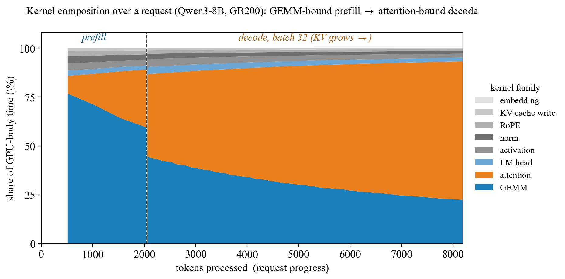
As shown in Table 2, our predictor’s advantage concentrates in the memory-bound and attention kernels. In real traces, however, GEMM accounts for a large share of kernel runtime, so the realized end-to-end improvement may be smaller than the per-kernel mean suggests.

As a request progresses, the kernel composition shifts substantially. Figure 8 shows an example. This is why simple calculation based on a fixed kernel decomposition is inaccurate.

7.2. Accurate In-Distribution Kernel Latency Prediction

Table 4. In-distribution per-kernel accuracy on NVIDIA GB200 (MAPE, lower is better). KernelSight-LM uses Tier B (§5.5): per-shape efficiency interpolated over the measured grid. AIConfigurator either interpolates a measured operator-level table or, for the elementwise/memory kernels, falls back to a fixed analytical model (query_mem_op $=\text{bytes}/(0.8\,\text{BW})+3\,\mu s$).

Kernel family	AIConfig.	Ours	Improv.
Operators they measure (table interpolation)
GEMM	02.8	2.6	$1.1\times$
Attention (decode)	11.3	3.6	$3.1\times$
Attention (prefill)	21.3	9.4	$2.3\times$
LM head	16.2	4.7	$3.4\times$
Kernels they model analytically (query_mem_op)
RMSNorm	29.9	2.7	$11\times$
RoPE	31.7	3.8	$8.3\times$
SiLU$\times$Mul (act.)	29.0	3.5	$8.3\times$
KV-cache write	43.1	3.3	$13\times$
Embedding	64.1	0.9	$71\times$
Mean	27.7	3.8	$7.3\times$

Table 4 compares Tier B against AIConfigurator (Xu et al., 2026) on GB200. The advantage comes from two distinct mechanisms, corresponding to the two ways an operator-level system loses resolution.

Completeness: measured kernels vs. an analytical shortcut.

Because AIConfigurator optimizes deployment configurations, where GEMMs and attention dominate runtime, it does not measure the small elementwise and memory kernels at all. RMSNorm, RoPE, the activation, the KV-cache write, and the embedding are routed through a single closed form, $\text{bytes}/(0.8\,\text{BW})+3\,\mu s$. This bakes in one fixed achieved-bandwidth fraction ($0.8$) and one fixed launch floor ($3\,\mu s$) for every kernel and shape; the measured ground truth violates both (per-family bias $0.73$–$1.64\times$). By measuring these kernels and learning a per-shape efficiency, KernelSight-LM cuts their error from $29$–$64\%$ to under $4\%$, a $\sim$$10\times$ gain that exists purely because we collect data the operator-level system never does.

Granularity: the efficiency target.

For the operators AIConfigurator does measure, the remaining advantage comes from what is interpolated. As described in §5.5, we let the roofline carry the order-of-magnitude scale and interpolate only the bounded efficiency residual, which is far smoother than a raw-latency surface that ranges over the LM head’s token count or attention’s sequence and KV length. Both systems use the same measured data, yet attention and the LM head still improve $2$–$3.5\times$. GEMM is the lone tie: a single, well-conditioned kernel whose latency surface is already smooth, so raw-latency interpolation is as good as ours.

Accuracy as a symptom.

These gains are a symptom of the deeper design difference established in §5.5: kernel-level prediction records the kernel that actually ran and is strictly more expressive. It aggregates up to any operator, recomposes unmeasured configurations, and (§5.4) transfers across GPU generations, none of which an operator table supports.

Translation to end-to-end improvement.

Per-kernel accuracy does not translate one-to-one end-to-end: AIConfigurator’s on-device, multi-trace calibration closes much of the decode-body gap there (§7.3), where the two are comparable.

Figure 9. GB200 real-vs-sim accuracy across select serving runs (models $\times$ TP $\times$ request rate) and three metrics. Tier A is zero-shot (cross-gen efficiency model plus a portable launch overhead, no GB200 host data); Tier B adds target-device microbenchmarks and a clean per-model host calibration. Each row is one $(\text{model},\text{TP},\text{request-rate})$ run and each column one serving metric; cell color encodes the median absolute percent error for that run and metric, clipped at 30% (darker = larger error).

7.3. End-to-end Inference Performance Prediction

Table 3 reports the distribution of per-request prediction error on GB200 across various serving runs spanning different model families, sizes, and tensor parallelism, and Figure 9 shows the corresponding per-run accuracy heatmap. For each cut, we give the median request error (p50) and the tail (p90 and p99); this shows more clearly how the prediction mechanisms compare. We evaluate two tiers of KernelSight-LM against AIConfigurator; Vidur is omitted and discussed separately below. KernelSight-LM is the most accurate while using the least target data in almost all cases.

TPOT Decode latency is predicted tightly. Tier B’s typical request is within 6% and its worst within 33%; even the zero-shot Tier A holds a 12% median (36% at p99). AIConfigurator is slightly better than ours in the decode body (5% median), likely because AIConfigurator is calibrated on-device from multiple run traces, while our Tier B uses only a short microbenchmark.

Vidur collapses to a 436% median error: its profiles use a different mode than actual vLLM runs, so it predicts a flat decode step several times the real graphed latency in every case. We omit Vidur from the table, as its predictions are uniformly far from the measured values.

TTFT Time-to-first-token is harder. Our predictors track the typical request well (14–15% median) but have a long tail (81% at p99). The worst cases are all long-context prefills (19–23k tokens), where attention is the least-transferable kernel. The gap to the external estimators is sharpest here, and it is structural, not a tail effect: AIConfigurator’s 59% median and Vidur’s 56% median both stem from having no host-overhead model, which makes their TTFT predictions effectively unusable.

Short prompts are dominated by admission, framing, and launch overhead, while long, compute-bound prompts are dominated more by GPU compute. KernelSight-LM represents these overheads explicitly in its discrete-event composition, making its typical-case TTFT roughly $4\times$ more accurate than either baseline.

Throughput Output throughput is the metric KernelSight-LM predicts most accurately (p50 at 3.0% MAPE). More specifically, the error is below 1% under light load, where throughput is arrival-limited, and rises to only 8% at saturation, where the simulator must reproduce the server’s true sustained rate.

AIConfigurator can achieve similar accuracy (2.7% at p50) at light load or below saturation. Saturation is exactly where AIConfigurator’s design breaks down: as a GPU-bound capacity estimator, it lacks the mechanism to model host and scheduling in detail, so the error rate explodes.

8. Conclusions

We presented KernelSight-LM, a kernel-level latency prediction framework for LLM serving simulation that achieves cross-GPU generalization without requiring per-device profiling. By decomposing transformer execution into fundamental kernels, our approach predicts latencies on unseen GPUs using only their published specifications or, more accurately, with a small on-device microbenchmarking. Integrated with an execution simulator, KernelSight-LM enables rapid evaluation of serving configurations across diverse hardware by providing high-fidelity predictions on multiple metrics. Our experiments demonstrate that kernel-level prediction achieves better accuracy than profiling-based methods. Our simulator extensions further enable exploring a wider search space of optimal configurations and supporting hardware-software co-design.

Looking ahead, the main open problem is the limited cross-generation transfer of the attention efficiency factor, which motivates one-shot per-architecture attention calibration; further directions include extending the host model into the saturated regime and broadening interconnect coverage.

Appendix A Experimental Setup Details

A.1. Software Version

We use the NGC PyTorch container image (26.04-py3) with vLLM v0.19.0 and CUDA 13, which is portable across platforms.

A.2. Evaluation Metric

Mean Absolute Percentage Error: MAPE

(5) $$\mathrm{MAPE}=\frac{100\%}{n}\sum_{i=1}^{n}\left|\frac{\hat{y}_{i}-y_{i}}{y_{i}}\right|$$

Per-Request Absolute Percent Error

(6) $$e_{i}=100\%\cdot\frac{\lvert\hat{y}_{i}-y_{i}\rvert}{y_{i}}$$

Error Percentiles: p50, p90, p99

(7) $$\mathrm{P}_{p}=e_{(k)},\qquad k=\left\lceil\tfrac{p}{100}\,n\right\rceil,\qquad e_{(1)}\leq e_{(2)}\leq\dots\leq e_{(n)}$$

A.3. GPUs and EC2 Instances

Table 5. GPUs used in our analysis and evaluation. They are deployed on AWS and the Boston University Shared Computing Clusters (BU SCC). BF16 throughput is dense. Memory bandwidth is per GPU. Peaks vary by SKU/clocks.

GPU	Instance	GPUs	Arch	Year	Mem / GPU	BW / GPU	BF16 TC	Mem type & interconnect
A100-40GB	p4d.24xlarge	8	Ampere	2020	40 GB	$\sim$1.56 TB/s	$\sim$312 TFLOPS	HBM2e; NVLink
A100-80GB-SXM4	p4de.24xlarge	8	Ampere	2020	80 GB	$\sim$2.04 TB/s	$\sim$312 TFLOPS	HBM2e; NVLink
A10G	g5.48xlarge	8	Ampere	2021	24 GB	$\sim$0.60 TB/s	$\sim$70 TFLOPS	GDDR6; PCIe
H100-80GB	p5.48xlarge	8	Hopper	2022	80 GB	$\sim$3.35 TB/s	$\sim$989 TFLOPS	HBM3; NVLink
H200-141GB	p5e.48xlarge	8	Hopper	2024	141 GB	$\sim$4.8 TB/s	$\sim$989 TFLOPS	HBM3e; NVLink
L4	g6.48xlarge	8	Ada Lovelace	2023	24 GB	$\sim$0.30 TB/s	$\sim$121 TFLOPS	GDDR6; PCIe
GB200	p6e-gb200.36xlarge	4	Blackwell	2024	192 GB	$\sim$8.0 TB/s	$\sim$2250 TFLOPS	HBM3e; NVLink-5
A40	BU SCC	4	Ampere	2020	48 GB	$\sim$0.70 TB/s	$\sim$150 TFLOPS	GDDR6; PCIe
A100-80GB-PCIe	BU SCC	4	Ampere	2021	80 GB	$\sim$1.94 TB/s	$\sim$312 TFLOPS	HBM2e; PCIe
L40S	BU SCC	4	Ada Lovelace	2023	48 GB	$\sim$0.86 TB/s	$\sim$362 TFLOPS	GDDR6; PCIe
H200-NVL	BU SCC	4	Hopper	2024	141 GB	$\sim$4.8 TB/s	$\sim$836 TFLOPS	HBM3e; NVLink
GB10 (RTX Spark)	Local Deployment	1	Blackwell	2025	128 GB	$\sim$0.27 TB/s	$\sim$125 TFLOPS	LPDDR5X; NVLink-C2C
RTX 5090	Local Deployment	1	Blackwell	2025	32 GB	$\sim$1.79 TB/s	$\sim$419 TFLOPS	GDDR7; PCIe

A.4. Models and Variants

Table 6. Model families and variants used across profiling, analysis, and evaluation.

Family	Developer	Variants (parameters)	TP
Llama (Grattafiori et al., 2024)	Meta	3.2-1B, 3.2-3B, 3.1-8B, 3.3-70B	1,2,4
Qwen (Qwen et al., 2025; Yang et al., 2025)	Alibaba	2.5-0.5B, 3-4B, 3-8B, 3-14B, 3-32B	1,2,4
DeepSeek (Bi et al., 2024; Guo et al., 2024)	DeepSeek-AI	LLM-7B, Coder-33B, LLM-67B	1,2,4
Phi (Gunasekar et al., 2023; Microsoft et al., 2025; Abdin et al., 2024)	Microsoft	Phi-2 (2.7B), Phi-4-mini (3.8B), Phi-4 (14B)	1
Gemma (Team et al., 2024)	Google	Gemma-2-9B	1
Mistral (Jiang et al., 2023)	Mistral AI	7B-Instruct-v0.3	1

Appendix B Limitations

B.1. Cross-Generation Kernel Prediction Challenge

Our predictor factors each kernel’s latency using the efficiency factor, $\eta$. This is a learned, dimensionless efficiency residual. Cross-generation prediction (Tier A) therefore rests on a single assumption: that $\eta$, fit on a set of training GPUs, transfers to an unseen target as claimed in (Lee et al., 2025). In practice, this assumption holds more weakly than prior work suggests.

Figure 10. The cross-generation test. Per-kernel $\eta=\text{measured}/\text{roofline}$ versus each family’s dominant shape parameter, across six GPUs. The five analysis devices are gray; GB200 (blue) is the held-out target. Where GB200’s curve lies within the analysis envelope (GEMM), $\eta$ interpolates; where it lies apart (attention, KV-cache, RoPE), $\eta$ is device-specific and cannot be recovered from the other devices. Dashed: GB200’s second dispatched attention kernel.

Figure 10 performs the experiment directly: we hold out GB200 and ask whether the analysis devices bracket its efficiency curve. For compute-bound GEMM, the target lies inside the analysis envelope, so interpolating $\eta$ recovers it. For the memory-bound families and especially attention, the GB200 curve sits well above the cluster: its $\eta$ is set by an achieved-bandwidth ceiling that does not scale with peak bandwidth, and for attention by the specific kernel the engine dispatches (the dashed line is a second GB200 attention kernel with a markedly different curve). Neither is observable from the analysis devices.

Figure 11 reduces each family to two numbers: the magnitude of $\eta$ (how far the multiplier departs from $1$, i.e. how much of the latency the roofline fails to explain) and its cross-device spread (its portability). The families separate cleanly. GEMM occupies the safe corner ($\eta\!\approx\!1.3$, spread $1.3\times$): the roofline does the work and the residual ports. Both attention variants occupy the opposite corner ($\eta\!\approx\!3$–$3.5$, spread up to $3.8\times$): the multiplier carries the physics and is device-specific. The diagonal between them is the core limitation, the families for which the learned efficiency factor matters most are precisely those for which it is least transferable.

Figure 11. When $\eta$ extrapolates. Each family placed by $\eta$ magnitude (geomean over devices; $1=$ roofline exact) and cross-device spread (max/min; $1=$ portable). The safe region (blue) holds families where the roofline is accurate and $\eta$ ports; the danger region (orange) holds those where $\eta$ both carries the prediction and varies across devices.

Two failure modes follow. When $\eta$ is far from $1$, the roofline acts as a normalizer rather than a model, and accuracy depends entirely on the residual; when $\eta$ varies several-fold across devices, no dimensionless feature combination recovers it for an unseen generation (the best linear combination of all shape features still leaves a large device-specific offset on these families). This is tolerable for GEMM and the lighter memory-bound kernels, but not for attention, where closing the gap requires at least one serving-matched measurement on each new architecture rather than pure extrapolation.

Appendix C Behavior at saturation

Another limitation is that the TTFT accuracy degrades as the offered rate approaches sustained capacity. Normalizing load as $\rho=\lambda/\mu$ (offered throughput over measured capacity), our TTFT error rises from $15\%$ to $22\%$ for $\rho\!\lesssim\!0.9$ but reaches $74\%$ at $\rho\!\approx\!1.2$, while TPOT and throughput errors stay $\leq\!13\%$ and $\leq\!7\%$.

This is because at high utilization, the request queue builds up. This inflates $13\%$ per-step errors into a $74\%$ TTFT error that no service-rate-based method can resolve. In practice this regime rarely matters: latency-SLO-oriented deployments typically operate at $\rho\!\approx\!0.6$–$0.8$. Because our simulator is accurate below saturation, it remains useful as a practical reference.

Figure 12. Prediction error vs. offered load (One run of Qwen3, TP1, GB200).