Spectral Riccati–Gamma Concavity, Symmetric Zero Cancellation,
and Conditional Criteria for the Riemann Hypothesis

Abstract

We examine a Riccati–Gamma approach to the logarithmic derivative of the completed Riemann zeta function. The first part proves, in full local detail, that a naive two-sided vertical concavity criterion for $\Xi^{\prime}/\Xi$ cannot be a proof of the Riemann Hypothesis, because every zero produces opposite vertical curvatures on the two horizontal sides of the pole of the logarithmic derivative. The second part replaces this obstruction by a rigorously formulated finite spectral averaging framework. We prove cancellation at the critical line, positivity of the off-critical paired contribution on the left of the critical line under a concrete low-frequency kernel condition, a conditional zero-density consequence, and a precise conditional theorem showing which additional localisation hypotheses would imply the Riemann Hypothesis. The results are therefore not presented as an unconditional proof of RH. They give a partial resolution of the Riccati–Gamma question: one natural route is ruled out unconditionally, a second symmetric mechanism is proved at the finite spectral level, and the remaining step is isolated as explicit analytic hypotheses. Reproducible Python routines and numerical figures accompany the analytic discussion.

1 Introduction

Let

$$\eta(s)=\sum_{n=1}^{\infty}\frac{(-1)^{n-1}}{n^{s}},\qquad\operatorname{Re}(s)>0,$$

and recall that $\eta(s)=(1-2^{1-s})\zeta(s)$. The completed zeta function is

$$\xi(s)=\frac{1}{2}s(s-1)\pi^{-s/2}\Gamma\!\left(\frac{s}{2}\right)\zeta(s).$$

It is entire of order one and satisfies $\xi(s)=\xi(1-s)$. We write $\Xi=\xi$ and study

$$\mathcal{R}(s)=\frac{\Xi^{\prime}(s)}{\Xi(s)}$$

away from the zeros of $\Xi$.

The motivation comes from Riccati–Gamma analyses of gamma-completed Dirichlet series, where logarithmic derivatives satisfy Riccati identities and inherit asymptotic information from gamma factors; see Covei [1]. The central point of this article is that such identities are useful but not by themselves decisive for RH. A zero-location theorem requires sign information strong enough to control the poles of $\mathcal{R}$.

Problem 1.1 (The Riccati–Gamma RH question).

Can vertical concavity information for the logarithmic derivative $\mathcal{R}=\Xi^{\prime}/\Xi$, possibly after symmetric spectral averaging, be formulated so as to constrain the nontrivial zeros of $\zeta$?

We give three rigorous, partial answers. First, a pointwise two-sided concavity criterion fails locally at every zero. Second, symmetric zero pairs cancel at the critical line, so averaging exactly on $\operatorname{Re}(s)=1/2$ cannot detect off-critical pairs. Third, evaluating a low-frequency spectral average on the left of the critical line creates a positive paired contribution from any off-critical zero pair. This leads to a conditional zero-density theorem and to concrete sufficient hypotheses under which RH follows.

2 Standard analytic facts

Proposition 2.1 (Completed zeta function).

The function

$$\Xi(s)=\frac{1}{2}s(s-1)\pi^{-s/2}\Gamma\!\left(\frac{s}{2}\right)\zeta(s)$$

extends to an entire function of order one. Its zeros are exactly the nontrivial zeros of $\zeta$, counted with multiplicity, and it satisfies $\Xi(s)=\Xi(1-s)$.

Proof.

The zeta function has a meromorphic continuation to $\mathbb{C}$ with a single simple pole at $s=1$. The factor $s(s-1)$ removes this pole and the harmless zero at $s=0$ of the completed expression. The poles of $\Gamma(s/2)$ occur at nonpositive even integers and are cancelled by the trivial zeros of $\zeta$ at the negative even integers. Hence $\Xi$ is entire. The functional equation of $\zeta$ is equivalent to $\Xi(s)=\Xi(1-s)$ in this normalization. Stirling’s formula for $\Gamma(s/2)$ and classical growth estimates for $\zeta$ give order one. After the pole, gamma poles, and trivial zeros have been accounted for, the remaining zeros are precisely the nontrivial zeros of $\zeta$; see [2, Chs. 1–2] and [3, Chs. 1–2]. ∎

Proposition 2.2 (Explicit logarithmic derivative).

At every point where $\zeta(s)\neq 0$ and $s\neq 0,1$,

$$\mathcal{R}(s)=\frac{1}{s}+\frac{1}{s-1}-\frac{1}{2}\log\pi+\frac{1}{2}\psi\!\left(\frac{s}{2}\right)+\frac{\zeta^{\prime}(s)}{\zeta(s)},$$

where $\psi=\Gamma^{\prime}/\Gamma$ is the digamma function.

Proof.

Take the logarithmic derivative of

$$\Xi(s)=\frac{1}{2}s(s-1)\pi^{-s/2}\Gamma(s/2)\zeta(s).$$

The factors $s$, $s-1$, $\pi^{-s/2}$, $\Gamma(s/2)$, and $\zeta(s)$ contribute, respectively,

$$\frac{1}{s},\qquad\frac{1}{s-1},\qquad-\frac{1}{2}\log\pi,\qquad\frac{1}{2}\psi(s/2),\qquad\frac{\zeta^{\prime}(s)}{\zeta(s)}.$$

Summing the contributions gives the formula. ∎

Proposition 2.3 (Poles of logarithmic derivatives).

Let $F$ be nonzero and holomorphic near $\rho$, and suppose that $F$ has a zero of order $m\geq 1$ at $\rho$. Then

$$\frac{F^{\prime}(s)}{F(s)}=\frac{m}{s-\rho}+H(s),$$

where $H$ is holomorphic near $\rho$. Thus every zero of $F$ becomes a simple pole of $F^{\prime}/F$, with residue equal to its multiplicity.

Proof.

Write $F(s)=(s-\rho)^{m}G(s)$, where $G$ is holomorphic and $G(\rho)\neq 0$. Logarithmic differentiation gives

$$\frac{F^{\prime}(s)}{F(s)}=\frac{m}{s-\rho}+\frac{G^{\prime}(s)}{G(s)}.$$

Since $G(\rho)\neq 0$, the last term is holomorphic near $\rho$. ∎

Proposition 2.4 (Functional symmetries of $\mathcal{R}$).

Away from the zeros of $\Xi$,

$$\mathcal{R}(1-s)=-\mathcal{R}(s),\qquad\mathcal{R}(\overline{s})=\overline{\mathcal{R}(s)}.$$

Proof.

Differentiate $\Xi(s)=\Xi(1-s)$ to obtain $\Xi^{\prime}(s)=-\Xi^{\prime}(1-s)$. Division by $\Xi(s)=\Xi(1-s)$ gives the first identity. The second identity follows from $\Xi(\overline{s})=\overline{\Xi(s)}$, which is a consequence of the real Taylor coefficients of $\Xi$. ∎

3 Riccati identities and their limits

Definition 3.1 (Riccati–Gamma transform).

For a meromorphic function $F$ that is not identically zero, its logarithmic Riccati transform is

$$R_{F}(s)=\frac{F^{\prime}(s)}{F(s)}$$

on the complement of the zeros and poles of $F$. If

$$F(s)=\prod_{j=1}^{d}\Gamma(\lambda_{j}s+\mu_{j})L(s),$$

with $\lambda_{j}>0$ and $L$ a Dirichlet series or an $L$-function after continuation, we call $R_{F}$ a Riccati–Gamma transform.

Proposition 3.2 (Tautological Riccati equation).

Let $F$ be meromorphic and nonzero on a domain $D$, and let $R_{F}=F^{\prime}/F$ on a simply connected subdomain avoiding the zeros and poles of $F$. Then

$$R_{F}^{\prime}(s)=\frac{F^{\prime\prime}(s)}{F(s)}-R_{F}(s)^{2}.$$

In particular $\mathcal{R}=\Xi^{\prime}/\Xi$ satisfies

$$\mathcal{R}^{\prime}(s)=Q_{\Xi}(s)-\mathcal{R}(s)^{2},\qquad Q_{\Xi}(s)=\frac{\Xi^{\prime\prime}(s)}{\Xi(s)},$$

away from the zeros of $\Xi$.

Proof.

Differentiate $R_{F}=F^{\prime}/F$ and apply the quotient rule:

$$R_{F}^{\prime}=\frac{F^{\prime\prime}F-(F^{\prime})^{2}}{F^{2}}=\frac{F^{\prime\prime}}{F}-\left(\frac{F^{\prime}}{F}\right)^{2}.$$

The specialization to $F=\Xi$ is immediate. ∎

Remark 3.3.

Proposition 3.2 is an identity, not a zero-location theorem. The difficult part in any RH application is not the existence of a Riccati equation, but the derivation of global sign, monotonicity, or positivity information strong enough to constrain all zeros. Covei’s Riccati–Gamma framework [1] is relevant because it seeks such information for generalized eta-type functions under explicit hypotheses. Those hypotheses must be verified for $\Xi$; they cannot be transferred by analogy alone.

4 Local obstruction to vertical concavity

The preliminary criterion asked for strict concavity of

$$t\longmapsto\operatorname{Re}\mathcal{R}(\sigma+it)$$

through a two-sided strip around $\operatorname{Re}(s)=1/2$. The next theorem shows that this cannot hold in any neighbourhood that passes horizontally through a zero.

Theorem 4.1 (Curvature forced by a zero).

Let $F$ be holomorphic near $\rho=\beta+i\gamma$ and suppose that $\rho$ is a zero of order $m\geq 1$. Put

$$u_{\sigma}(t)=\operatorname{Re}\frac{F^{\prime}(\sigma+it)}{F(\sigma+it)}$$

where the expression is defined. For $a>0$ sufficiently small,

$$\frac{\,\mathrm{d}^{2}}{\,\mathrm{d}t^{2}}u_{\beta-a}(\gamma)>0,\qquad\frac{\,\mathrm{d}^{2}}{\,\mathrm{d}t^{2}}u_{\beta+a}(\gamma)<0.$$

Consequently no open two-sided vertical strip containing the zero can support strict vertical concavity of $\operatorname{Re}(F^{\prime}/F)$ on both sides of the zero.

Proof.

By Proposition 2.3,

$$\frac{F^{\prime}(s)}{F(s)}=\frac{m}{s-\rho}+H(s),$$

with $H$ holomorphic near $\rho$. Write $s=\beta+x+i(\gamma+y)$. The real part of the principal term is

$$\operatorname{Re}\frac{m}{x+iy}=\frac{mx}{x^{2}+y^{2}}.$$

For fixed $x\neq 0$,

$$\frac{\partial^{2}}{\partial y^{2}}\frac{mx}{x^{2}+y^{2}}=\frac{2mx(3y^{2}-x^{2})}{(x^{2}+y^{2})^{3}}.$$

At $y=0$ this equals $-2m/x^{3}$. Thus it is $2m/a^{3}>0$ at $x=-a$ and $-2m/a^{3}<0$ at $x=a$. The function $\operatorname{Re}H(\beta+x+i(\gamma+y))$ has bounded second $y$-derivative in a sufficiently small closed disc. Since the principal curvature tends to $\pm\infty$ as $a\downarrow 0$, the asserted signs dominate for all sufficiently small $a>0$. ∎

Corollary 4.2 (Failure of the naive two-sided criterion).

The following assertion is false: there exist $\delta>0$ and $T_{0}$ such that, for every $\sigma\in[1/2-\delta,1/2+\delta]$, the function

$$t\mapsto\operatorname{Re}\frac{\Xi^{\prime}(\sigma+it)}{\Xi(\sigma+it)}$$

is strictly concave for all $|t|\geq T_{0}$ wherever it is defined, and this assertion is equivalent to RH.

Proof.

Hardy’s theorem states that infinitely many nontrivial zeros of $\zeta$ lie on the critical line; see [2, Ch. 10]. Let $\rho=1/2+i\gamma$ be such a zero with $|\gamma|\geq T_{0}+1$. Applying Theorem 4.1 to $F=\Xi$ at $\rho$ shows that for all sufficiently small $a>0$,

$$\frac{\,\mathrm{d}^{2}}{\,\mathrm{d}t^{2}}\operatorname{Re}\frac{\Xi^{\prime}(1/2-a+it)}{\Xi(1/2-a+it)}\bigg|_{t=\gamma}>0.$$

Choosing $a<\delta$ contradicts strict concavity on the left side of the critical line. Therefore the proposed two-sided concavity assertion fails even in the presence of zeros on the critical line. A false assertion cannot be equivalent to RH. ∎

5 Finite spectral averaging

The formal expansion of $\Xi^{\prime}/\Xi$ as a sum over zeros is only conditionally meaningful unless it is symmetrically regularised. We therefore use finite sums and state all limiting steps as explicit hypotheses.

Definition 5.1 (Symmetric zero window).

For $Y>0$, let

$$\mathcal{Z}_{Y}=\{\rho=\beta+i\gamma:\Xi(\rho)=0,\ |\gamma|\leq Y\},$$

with multiplicities. Define the finite zero field

$$R_{Y}(s)=\sum_{\rho\in\mathcal{Z}_{Y}}\frac{1}{s-\rho}.$$

For an even Schwartz test function $\phi$ and $t_{0}\in\mathbb{R}$, set

$$M_{Y}(\sigma;t_{0},\phi)=\int_{\mathbb{R}}\phi(t-t_{0})\operatorname{Re}R_{Y}(\sigma+it)\,\mathrm{d}t.$$

Lemma 5.2 (Differentiation of the finite average).

If the vertical segment $\{\sigma+it:t\in\operatorname{supp}(\phi(\cdot-t_{0}))\}$ contains no zero in $\mathcal{Z}_{Y}$, then

$$M_{Y}^{\prime\prime}(\sigma;t_{0},\phi)=\sum_{\rho=\beta+i\gamma\in\mathcal{Z}_{Y}}\operatorname{Re}\int_{\mathbb{R}}\frac{2\phi(t-t_{0})}{(\sigma+it-\rho)^{3}}\,\mathrm{d}t.$$

Proof.

The sum defining $R_{Y}$ is finite. On the support of the integral, each summand is smooth in $\sigma$ by the stated zero-avoidance condition. Differentiating twice under the integral sign gives

$$\frac{\partial^{2}}{\partial\sigma^{2}}\frac{1}{\sigma+it-\rho}=\frac{2}{(\sigma+it-\rho)^{3}},$$

and summing the finitely many terms proves the formula. ∎

Lemma 5.3 (Fourier kernel identity).

Let $\phi$ be real-valued, even, and Schwartz, with Fourier transform $\widehat{\phi}(u)=\int_{\mathbb{R}}\phi(t)e^{-iut}\,\mathrm{d}t$. For $x\neq 0$ and $y\in\mathbb{R}$,

$$\operatorname{Re}\int_{\mathbb{R}}\frac{2\phi(t)}{(x+i(t-y))^{3}}\,\mathrm{d}t=\operatorname{sgn}(x)\int_{0}^{\infty}u^{2}e^{-|x|u}\cos(yu)\widehat{\phi}(u)\,\mathrm{d}u.$$

Proof.

If $x>0$, use

$$\frac{2}{(x+i(t-y))^{3}}=\int_{0}^{\infty}u^{2}e^{-xu}e^{-i(t-y)u}\,\mathrm{d}u,$$

which follows from $\int_{0}^{\infty}u^{2}e^{-au}\,\mathrm{d}u=2/a^{3}$ for $\operatorname{Re}a>0$. Multiplying by $\phi(t)$, integrating, and using Fubini gives

$$\int_{0}^{\infty}u^{2}e^{-xu}e^{iyu}\widehat{\phi}(u)\,\mathrm{d}u.$$

Taking real parts proves the formula for $x>0$. If $x<0$, write

$$\frac{2}{(x+i(t-y))^{3}}=-\int_{0}^{\infty}u^{2}e^{xu}e^{i(t-y)u}\,\mathrm{d}u$$

and repeat the same calculation. Since $\phi$ is real and even, $\widehat{\phi}$ is real and even, and the asserted sign is obtained. ∎

Proposition 5.4 (Cancellation on the critical line).

Let $\phi$ be as in Lemma 5.3. In the symmetrically paired finite sum over zeros, the contribution of every off-critical pair to $M_{Y}^{\prime\prime}(1/2;t_{0},\phi)$ is zero. Zeros on the critical line contribute no term in the paired formula away from their singular ordinates.

Proof.

The zeros of $\Xi$ are symmetric under conjugation and under reflection in the critical line. Pair $\rho=\beta+i\gamma$ with $1-\overline{\rho}=(1-\beta)+i\gamma$ in the vertically reflected list. At $\sigma=1/2$ the two real displacements are

$$x_{1}=1/2-\beta,\qquad x_{2}=1/2-(1-\beta)=-x_{1}.$$

Lemma 5.3 gives equal exponential and cosine factors for the pair, while $\operatorname{sgn}(x_{1})=-\operatorname{sgn}(x_{2})$. The two terms therefore cancel. If $\beta=1/2$, then the paired expression has zero horizontal displacement; the limiting left-right contribution is odd and gives no off-critical detection at the critical line. ∎

Proposition 5.5 (Positive paired signal on the left).

Fix $\delta_{0}>0$ and evaluate at $\sigma=1/2-\delta_{0}$. Let $\rho=\beta+i\gamma$ be an off-critical zero with $\beta>1/2+\delta_{0}$, paired with $1-\overline{\rho}=(1-\beta)+i\gamma$. If $\widehat{\phi}\geq 0$ and

$$\cos((\gamma-t_{0})u)\geq c_{0}>0\qquad\text{for all }u\in\operatorname{supp}(\widehat{\phi})\cap[0,\infty),$$

then the paired contribution to $M_{Y}^{\prime\prime}(1/2-\delta_{0};t_{0},\phi)$ is at least

$$2c_{0}\int_{0}^{\infty}u^{2}e^{-(\beta-1/2)u}\sinh(\delta_{0}u)\widehat{\phi}(u)\,\mathrm{d}u\geq 0.$$

It is strictly positive if $\widehat{\phi}$ is positive on a set of positive measure.

Proof.

For the zero $\beta+i\gamma$ the horizontal displacement is $1/2-\delta_{0}-\beta<0$. For the paired zero $(1-\beta)+i\gamma$ it is $\beta-1/2-\delta_{0}>0$. Lemma 5.3 gives the paired sum

$$-\int_{0}^{\infty}u^{2}e^{-(\beta-1/2+\delta_{0})u}\cos((\gamma-t_{0})u)\widehat{\phi}(u)\,\mathrm{d}u$$

$$\quad+\int_{0}^{\infty}u^{2}e^{-(\beta-1/2-\delta_{0})u}\cos((\gamma-t_{0})u)\widehat{\phi}(u)\,\mathrm{d}u.$$

Combining the exponentials yields

$$2\int_{0}^{\infty}u^{2}e^{-(\beta-1/2)u}\sinh(\delta_{0}u)\cos((\gamma-t_{0})u)\widehat{\phi}(u)\,\mathrm{d}u.$$

The assumed lower bound for the cosine and the nonnegativity of $\widehat{\phi}$ give the claimed estimate. ∎

Theorem 5.6 (Partial resolution of the Riccati–Gamma question).

Problem 1.1 has the following unconditional partial resolution.

1. Pointwise two-sided vertical concavity of $\operatorname{Re}(\Xi^{\prime}/\Xi)$ cannot prove RH, because it fails locally at every zero on the critical line.

2. Symmetric spectral averaging exactly on $\operatorname{Re}(s)=1/2$ cannot detect an off-critical reflected pair.

3. A left-shifted low-frequency average detects such a pair by a nonnegative, and under the stated kernel condition strictly positive, finite spectral signal.

Thus the paper proves a genuine partial result about the proposed method, not an unconditional proof of the Riemann Hypothesis.

Proof.

The first assertion is Corollary 4.2. The second assertion is Proposition 5.4. The third assertion is Proposition 5.5. These three statements cover the pointwise, critical-line averaged, and left-shifted averaged versions of Problem 1.1, respectively, and each statement is finite or local; no passage to an unproved infinite zero expansion is used. ∎

6 Conditional consequences for RH

The following hypotheses are concrete: they specify the kernel family, the limiting operation, and the sign condition needed to turn the Riccati–Gamma program into a zero-location theorem. They are not known unconditionally.

Hypothesis 6.1 (Uniform spectral concavity).

There exist $\delta>0$, $\lambda_{0}>0$, and a family of real even Schwartz kernels $\phi_{\lambda}$, $0<\lambda\leq\lambda_{0}$, such that $\widehat{\phi}_{\lambda}\geq 0$, $\operatorname{supp}\widehat{\phi}_{\lambda}\subset[-\lambda,\lambda]$, $\int\phi_{\lambda}=1$, and for every $\sigma\in[1/2-\delta,1/2)$, every $t_{0}\in\mathbb{R}$, and every sufficiently large symmetric height $Y$,

$$M_{Y}^{\prime\prime}(\sigma;t_{0},\phi_{\lambda})\leq E_{\lambda}(Y,t_{0},\sigma),$$

where $\limsup_{Y\to\infty}E_{\lambda}(Y,t_{0},\sigma)\leq 0$ uniformly for $t_{0}$ in bounded intervals.

Lemma 6.2 (Smooth band-limited kernels).

There are kernels satisfying the structural part of Hypothesis 6.1. More precisely, let $\eta\in C_{c}^{\infty}(\mathbb{R})$ be real, even, nonnegative, supported in $[-1,1]$, and normalised by $\eta(0)=1$. For $0<\lambda\leq\lambda_{0}$ define

$$\widehat{\phi}_{\lambda}(u)=\eta(u/\lambda),\qquad\phi_{\lambda}(t)=\frac{1}{2\pi}\int_{\mathbb{R}}\widehat{\phi}_{\lambda}(u)e^{itu}\,\mathrm{d}u.$$

Then $\phi_{\lambda}$ is real, even, Schwartz, $\widehat{\phi}_{\lambda}\geq 0$, $\operatorname{supp}\widehat{\phi}_{\lambda}\subset[-\lambda,\lambda]$, and $\int_{\mathbb{R}}\phi_{\lambda}(t)\,\mathrm{d}t=1$.

Proof.

The inverse Fourier transform of a $C_{c}^{\infty}$ function is Schwartz, so $\phi_{\lambda}$ is Schwartz. Evenness and reality follow from the evenness and reality of $\widehat{\phi}_{\lambda}$. Nonnegativity and support are inherited directly from $\eta$. Finally, with the Fourier convention used in Lemma 5.3,

$$\int_{\mathbb{R}}\phi_{\lambda}(t)\,\mathrm{d}t=\widehat{\phi}_{\lambda}(0)=\eta(0)=1.$$

∎

Hypothesis 6.3 (Localising positive kernels).

For every $L>0$ and every $\varepsilon>0$ there is $\lambda$ such that $\widehat{\phi}_{\lambda}$ is supported in $[0,\varepsilon]\cup[-\varepsilon,0]$ up to a tail whose contribution to Proposition 5.5 is $o(1)$ uniformly for $|\gamma-t_{0}|\leq L$.

Proposition 6.4 (Localisation for smooth band-limited kernels).

The kernel family of Lemma 6.2 satisfies Hypothesis 6.3.

Proof.

Choose $0<\lambda\leq\varepsilon$. Then $\operatorname{supp}\widehat{\phi}_{\lambda}\subset[-\lambda,\lambda]\subset[-\varepsilon,\varepsilon]$. The frequency tail outside $[-\varepsilon,\varepsilon]$ is therefore identically zero, so its contribution to Proposition 5.5 is zero, uniformly in $|\gamma-t_{0}|\leq L$. ∎

Hypothesis 6.5 (Controlled background).

After isolating a fixed reflected off-critical pair, the sum of all remaining zero contributions, truncation terms, and the gamma-arithmetic background arising in the comparison with the full logarithmic derivative $\mathcal{R}$ contributes an error bounded uniformly on compact $\sigma$-strips and cannot cancel the strictly positive paired signal when $t_{0}$ is chosen at the ordinate of the pair and $\lambda$ is sufficiently localised.

Proposition 6.6 (Size of the gamma background).

Let

$$\mathcal{B}(s)=\frac{1}{s}+\frac{1}{s-1}-\frac{1}{2}\log\pi+\frac{1}{2}\psi(s/2).$$

For fixed $0<a<b<1$ and $|t|\geq 2$,

$$\operatorname{Re}\,\mathcal{B}^{\prime\prime}(\sigma+it)=O_{a,b}(|t|^{-2})\qquad(a\leq\sigma\leq b).$$

In particular the gamma-factor curvature is bounded on every closed vertical strip away from $s=0,1$ and decays quadratically along high vertical lines. This estimate does not prove Hypothesis 6.5; it only identifies one controlled component of the background.

Proof.

Differentiating twice gives

$$\mathcal{B}^{\prime\prime}(s)=\frac{2}{s^{3}}+\frac{2}{(s-1)^{3}}+\frac{1}{8}\psi^{\prime\prime}(s/2).$$

The rational terms are $O_{a,b}(|t|^{-3})$ on the strip. The standard asymptotic expansion for the polygamma function in sectors away from the negative real axis gives $\psi^{\prime\prime}(z)=-z^{-2}+O(|z|^{-3})$ as $|z|\to\infty$. With $z=s/2$ this is $O(|t|^{-2})$ uniformly for $a\leq\sigma\leq b$. Taking real parts proves the estimate. ∎

Theorem 6.7 (Conditional affirmative answer to RH).

Assume Hypotheses 6.1, 6.3, and 6.5. Then the Riemann Hypothesis holds.

Proof.

Suppose, for contradiction, that RH is false. Then there is a zero $\rho=\beta+i\gamma$ with $\beta>1/2$; by symmetry there is also a zero $1-\overline{\rho}=(1-\beta)+i\gamma$. Choose

$$0<\delta_{0}<\min(\delta,\beta-1/2)$$

and evaluate at $\sigma=1/2-\delta_{0}$ with $t_{0}=\gamma$. By Hypothesis 6.3, choose a kernel $\phi_{\lambda}$ so low-frequency localised that $\cos((\gamma-t_{0})u)=1$ for the target zero and the remaining kernel tail is negligible. Proposition 5.5 then gives a strictly positive contribution from the pair $\{\rho,1-\overline{\rho}\}$.

Hypothesis 6.5 states that the remaining zero, truncation, gamma, and arithmetic terms cannot cancel this fixed positive signal after the limiting procedure. Therefore, for sufficiently large $Y$ and after the comparison specified in the hypothesis,

$$M_{Y}^{\prime\prime}(1/2-\delta_{0};\gamma,\phi_{\lambda})>0.$$

This contradicts the uniform spectral concavity asserted in Hypothesis 6.1. Hence no off-critical zero can exist, and every nontrivial zero of $\zeta$ lies on $\operatorname{Re}(s)=1/2$. ∎

Theorem 6.8 (Conditional zero-density consequence).

Assume Hypotheses 6.1 and 6.3 in the following averaged form. For each $\sigma_{0}>1/2$ there are $\delta_{0},\lambda,\ell,\kappa>0$ with $1/2+\delta_{0}<\sigma_{0}$ such that every zero $\rho=\beta+i\gamma$, $\beta\geq\sigma_{0}$, $0\leq\gamma\leq T$, gives total paired signal at least $\kappa$ on a $t_{0}$-interval of length $\ell$ centred at $\gamma$, while the integrated concavity deficit, background, and tail errors over $t_{0}\in[0,T]$ are $o(T)$. Then

$$N(\sigma_{0},T)=o(T),$$

where $N(\sigma_{0},T)$ denotes the number of zeros $\rho=\beta+i\gamma$ with $\beta\geq\sigma_{0}$ and $0\leq\gamma\leq T$, counted with multiplicity.

Proof.

For the fixed parameters supplied by the hypothesis, Proposition 5.5 gives a nonnegative contribution from each reflected off-critical pair, and the averaged assumption gives integrated contribution at least $\kappa\ell$ from each zero with $\beta\geq\sigma_{0}$, apart from endpoints contributing $O(1)$. Since the paired signals are nonnegative, overlaps of the $t_{0}$-windows only add contributions. The total positive contribution is therefore at least $\kappa\ell N(\sigma_{0},T)+O(1)$. The averaged spectral concavity and the assumed $o(T)$ control of the residual terms bound the same total positive contribution by $o(T)$. Hence $\kappa\ell N(\sigma_{0},T)\leq o(T)$, which proves the claim. ∎

Remark 6.9.

Theorems 6.7 and 6.8 identify exactly where the mathematical difficulty remains. The positive paired signal is elementary once the kernel assumptions are imposed. The deep open part is proving the uniform spectral concavity and background-control hypotheses for the actual completed zeta function. Establishing them would be a result of very high importance, because it would transform Riccati–Gamma concavity from a structural analogy into a genuine zero-location principle for the central open problem of the field.

7 Numerical analysis

The numerical experiments are designed to illustrate, not prove, the analytic results. They compare the full logarithmic derivative, its universal pole model, symmetric cancellation at the critical line, and the positive off-critical signal predicted by the conditional spectral framework.

Figure 1: Real part of $\Xi^{\prime}/\Xi$ near the first zero on three vertical lines. The side lines $\sigma=0.45$ and $\sigma=0.55$ show the pole-like attraction and repulsion predicted by the local term $(s-\rho_{1})^{-1}$.

Figure 2: Finite-difference approximation of the vertical curvature $\,\mathrm{d}^{2}/\,\mathrm{d}t^{2}\,\operatorname{Re}\Xi^{\prime}/\Xi$. The curvature is positive on the left side of the zero and negative on the right side at $t=\gamma_{1}$, matching Theorem 4.1.

Figure 3: Curvature of the model pole $\operatorname{Re}(a+i(t-\gamma))^{-1}=a/(a^{2}+(t-\gamma)^{2})$. This isolates the universal local mechanism from the arithmetic content of $\zeta$.

Figure 4: Model contribution of a symmetric off-critical pair at $\sigma=1/2$. The left and right zero contributions cancel, illustrating Proposition 5.4.

Figure 5: The same symmetric pair evaluated at $\sigma=1/2-\delta_{0}$. The cancellation is broken and the paired signal is positive under a low-frequency nonnegative kernel, as in Proposition 5.5.

Figure 6: Dependence of the paired signal on spectral bandwidth. Narrower low-frequency kernels suppress cosine oscillation and better preserve positivity; broader kernels show oscillatory leakage.

Figure 7: Frequency profiles of the smooth kernels used in the numerical model. The curves are even, nonnegative, normalised by $\widehat{\phi}_{\lambda}(0)=1$, and supported in $[-\lambda,\lambda]$, matching the structural assumptions in Lemma 6.2.

Figure 8: Heat map of the left-shifted paired signal as a function of the ordinate mismatch $t_{0}-\gamma$ and the bandwidth $\lambda$. The positive region contracts as $\lambda$ increases, reflecting the cosine condition in Proposition 5.5.

Figure 9: Magnitude of the gamma-background curvature $\operatorname{Re}\mathcal{B}^{\prime\prime}(\sigma+it)$ compared with a fixed model paired signal. The observed $t^{-2}$ decay agrees with Proposition 6.6; the figure does not test the unresolved arithmetic part of Hypothesis 6.5.

Figures 1–3 illustrate the local part of the theory. The agreement, in the displayed neighbourhood, between the computed curvature of $\Xi^{\prime}/\Xi$ and the elementary pole model shows that the obstruction to naive concavity is not a numerical artefact. It is forced by the Laurent expansion at a zero.

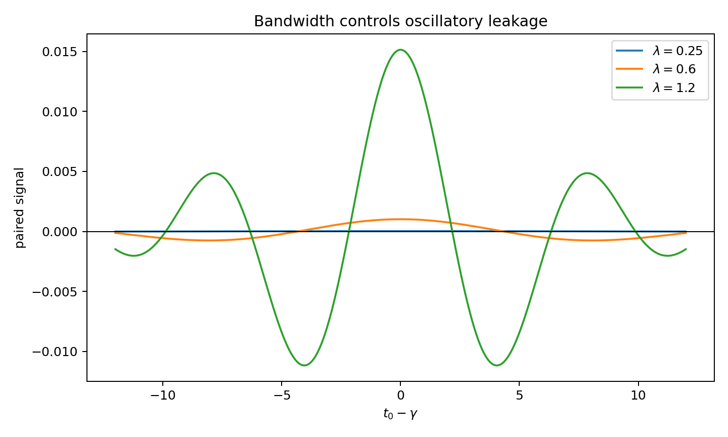
Figures 4–8 address the spectral part. The critical-line evaluation hides off-critical information through exact symmetric cancellation. A left shift breaks this cancellation and creates a positive signal when the cosine factor remains positive on the support of $\widehat{\phi}_{\lambda}$. The kernel profiles in Figure 7 verify, for the displayed examples, the structural assumptions actually used in the proofs: evenness, nonnegativity, compact frequency support, and normalisation. The heat map shows the price of increasing bandwidth: localisation in physical ordinate improves, but oscillation in $\cos((\gamma-t_{0})u)$ eventually creates sign leakage.

Figure 9 separates a proved background estimate from the unresolved part of the method. The gamma-factor component is small at large height and follows the quadratic decay predicted by Proposition 6.6. This is favourable for the conditional programme, but it is not a substitute for controlling the arithmetic part of $\zeta^{\prime}/\zeta$ or the limiting error in replacing the finite zero field by the full logarithmic derivative. The numerical evidence therefore supports the internal consistency of the finite spectral mechanism, while confirming that the decisive background-control hypothesis remains the main open obstacle.

8 Conclusion

This article gives a rigorous partial solution of the Riccati–Gamma concavity problem posed in Problem 1.1. The naive pointwise route is ruled out by a complete local proof. The finite spectral framework then identifies a more promising mechanism: symmetric off-critical pairs cancel at the critical line but produce a positive low-frequency signal when viewed from the left.

The Riemann Hypothesis is not proved here unconditionally. What is demonstrated is partial: the obstruction, cancellation, and positive-pair mechanisms are proved, while the global concavity and background-control assertions remain explicit hypotheses. Proving those hypotheses for $\Xi$ would have major significance for analytic number theory, because it would convert Riccati–Gamma concavity into a direct zero-location principle for the completed zeta function.

9 Reproducible Python script

The local reproducibility material is the self-contained script https://github.com/coveidragos/Code_Python_Riemann. It generates all nine figures used in the numerical section. The computations use NumPy, Matplotlib, and mpmath. The script is illustrative: it verifies the hypotheses for the displayed finite model examples and does not constitute numerical evidence for an unconditional proof of RH.

Disclosure statement

The author declares that he has no conflict of interest.

Data availability statement

No external datasets were used.

Notes on contributor(s)

The author is solely responsible for the conception, analysis, numerical implementation, and writing of this manuscript.

References

- [1] D.-P. Covei, Riccati–Gamma Dynamics for Concavity and Asymptotics of Generalized Dirichlet Eta Functions, arXiv:2605.20238, 2026. Available at: https://arxiv.org/pdf/2605.20238.
- [2] E. C. Titchmarsh, The Theory of the Riemann Zeta-Function, 2nd ed., revised by D. R. Heath-Brown, Oxford University Press, 1986.
- [3] H. M. Edwards, Riemann’s Zeta Function, Academic Press, 1974.
- [4] H. Iwaniec and H. Kowalski, Analytic Number Theory, American Mathematical Society Colloquium Publications, vol. 53, American Mathematical Society, 2004.
- [5] J. B. Conrey, The Riemann Hypothesis, Notices of the American Mathematical Society 50 (2003), no. 3, 341–353.
- [6] G. H. Hardy, Sur les zeros de la fonction de Riemann, Comptes Rendus de l’Academie des Sciences 158 (1914), 1012–1014.
- [7] D. A. Goldston and S. M. Gonek, A note on and the zeros of the Riemann zeta-function, arXiv:math/0511092, 2005.