A General Framework for Decision Trees via Bregman Divergences

Abstract

Decision trees are one of the fundamental tools in statistical learning due to their interpretability, flexibility, and their ability to adapt to nonlinear structures. Among them, the Classification and Regression Trees, introduced by Breiman, Friedman, Olshen, and Stone in 1984, became one of the most influential algorithms and remains one of the most widely used methods for classification and regression problems. On the other hand, Bregman divergences, introduced by Lev Bregman in 1967 in the context of convex optimization, provide a broad family of loss functions that naturally generalize the squared Euclidean distance. This family includes, among others, the Kullback–Leibler divergence, the Poisson divergence, and the Itakura–Saito divergence, as well as several losses associated with distributions belonging to the exponential family. Moreover, Bregman divergences possess a rich geometric structure and deep connections with convex analysis and information geometry. In this work, we propose a generalization of the CART paradigm based on Bregman divergences, thereby obtaining a broader family of decision trees adapted to different statistical models and underlying geometries. Although algorithms such as CART or classical implementations such as rpart incorporate different impurity criteria, these are usually introduced in an ad hoc manner for each specific model. In contrast, the Bregman divergence approach provides a unified framework that allows these criteria to be derived and interpreted from common convex and geometric principles. Beyond the algorithmic construction, we also investigate theoretical properties of these trees. In particular, we study how properties of the generating convex function — such as strong convexity or smoothness — influence impurity gains between parent and child nodes, as well as stability and consistency properties of the estimator.

Keywords: Decision trees, Bregman divergences, Tree-based methods, Exponential families, Convex optimization, Information geometry, Statistical learning, Nonparametric models

1 Introduction

Decision trees are among the most widely used tools in statistical learning due to their interpretability and flexibility. The classical CART (Classification and Regression Trees) algorithm, introduced by Breiman, Friedman, Olshen, and Stone in 1984 (Breiman et al. (1984)), became one of the most influential and widely used methods for classification and regression problems. When the goal is to predict a continuous response, regression trees are typically based on squared-error loss, whereas classification trees rely on criteria such as the misclassification error, entropy, or the Gini index.

In this work, we develop a general Bregman-divergence framework for CART in both regression and classification settings. These discrepancy measures were introduced by Lev Bregman in 1967 in Bregman (1967) in the context of convex programming and have since become fundamental tools in optimization, information geometry, and statistical learning. For two points $x$ and $y$ in a convex set $C$, and a strictly convex, differentiable function $\psi:C\to\mathbb{R}$ the Bregman divergence generated by $\psi$ between $x$ and $y$ is defined as:

$$D_{\psi}(x,y)=\psi(x)-\psi(y)-\langle\nabla\psi(y),x-y\rangle.$$

While the use of Bregman divergences has had a significant impact in clustering and related problems (Banerjee et al. (2005)), their role in decision tree methods has remained comparatively implicit. Classical decision trees, such as CART, rely on impurity measures including squared error, entropy, or the Gini index, each of which corresponds to a specific divergence. However, these criteria are typically introduced in a case-by-case manner, without explicitly leveraging the general structure provided by Bregman divergences. These approaches implicitly rely on the connection between exponential families and Bregman divergences, but do not emphasize the underlying geometric framework or its consequences for the analysis of splitting procedures. Moreover, in contrast to clustering, which seeks a global partition minimizing a given objective, decision trees construct partitions recursively using greedy splitting criteria. This sequential structure introduces new analytical challenges and requires a dedicated study of the split gain as a central object.

Several extensions of recursive partitioning methods have been proposed for responses arising from exponential-family models. In particular, model-based recursive partitioning and generalized linear model trees fit parametric models within each terminal node and recursively split the data according to parameter instability tests Zeileis et al. (2008); Hothorn and Zeileis (2015); Seibold et al. (2016). More recently, distributional trees have extended this framework by allowing all parameters of a distributional model to vary across the partition Schlosser et al. (2019). These approaches focus on local likelihood modeling and parameter heterogeneity across subpopulations. In contrast, the present work retains the classical CART paradigm of piecewise-constant prediction within terminal nodes and instead generalizes the impurity criterion itself. Our contribution is to show that a broad class of tree construction procedures can be formulated through Bregman divergences, yielding a unified geometric framework encompassing many classical splitting criteria as particular cases.

The present work makes this structure explicit within the CART framework. By formulating node impurity and split selection in terms of general Bregman divergences, we obtain a unified treatment encompassing a broad class of exponential-family models. The main contributions of the paper are threefold. First, we formulate CART impurity measures and split gains within a general Bregman framework. Second, we derive geometric characterizations of impurity reduction and establish connections with classical deviance-based criteria. Third, we investigate the resulting Bregman Trees through theoretical analysis and empirical studies. The remainder of the paper is organized as follows. Section 2 reviews the necessary background on exponential families and Bregman divergences. Section 3 provides a brief review of the CART methodology, including impurity measures, splitting criteria, and pruning procedures. Section 4 introduces the proposed Bregman Tree methodology and Section 5 discusses its theoretical properties. Section 6 reports simulation studies and a real-data application comparing Bregman Trees and CART. Finally, we conclude with a discussion and directions for future research.

2 Background on Bregman Divergences and Exponential Families

The construction of the proposed Bregman Trees relies on a close relationship between exponential-family distributions, convex analysis, and Bregman divergences. The aim of this section is to review these connections and establish the notation used throughout the paper. We start with the definition of Bregman divergences and some associated properties, then we present the exponential-family framework, and the associated convex conjugate functions. These concepts will serve as the basis for the impurity measures considered later in the tree-building procedure.

2.1 Bregman Divergences and some basic properties

Bregman divergences constitute a broad class of discrepancy measures generated by convex functions. They encompass many well-known loss functions used in statistics, machine learning, and information theory, including the squared loss, the Kullback–Leibler divergence, the logistic loss, the Itakura–Saito divergence, and the Mahalanobis distance. They were introduced by Lev Bregman in 1967 in the context of convex programming (Bregman (1967)). Since then, they have found numerous applications in areas such as information geometry, statistical learning, and convex optimization. Their importance stems from the fact that many statistical models and loss functions can be naturally expressed in terms of a suitable Bregman divergence. We begin by recalling the formal definition of a Bregman divergence and some of its fundamental properties.

Definition 1.

Let $\psi:C\to\mathbb{R}$ be a differentiable strictly convex function on $C\subset\mathbb{R}^{n}$ a convex set. The associated Bregman divergence $D_{\psi}:C\times C\to[0,+\infty)$ is defined as

$$D_{\psi}(x,y)=\psi(x)-\psi(y)-\langle\nabla\psi(y),x-y\rangle.$$

Example 1.

1. If $\psi(x)=x^{2}$ then $D_{\psi}(x,y)=(x-y)^{2}$ corresponds to the euclidean distance.

2. If ${\bf p}=(p_{1},\dots,p_{n})\geq{\bf 0},\sum p_{i}=1$ is a vector of probability and $\psi({\bf p})=\sum\limits_{i}p_{i}\log(p_{i})$ then $D_{\psi}({\bf p},{\bf q})=\sum\limits_{i}p_{i}\log\frac{p_{i}}{q_{i}}=D_{KL}({\bf p}||{\bf q})$ is the Kullback-Leibler divergence between vectors ${\bf p}$ and ${\bf q}$).

The Bregman divergence is exactly the error of the approximation between $\psi(x)$ and the linear approximation at $\psi(y)$ given by its tangent plane:

$$D_{\psi}(x,y)=\psi(x)-\big[\psi(y)+\langle\nabla\psi(y),x-y\rangle\big].$$

Another interpretation can be given by the approximation: assuming $\psi$ have derivatives of second order

$$D_{\psi}(x,y)\approx\frac{1}{2}(x-y)^{t}\nabla^{2}\psi(\zeta)(x-y)$$

where $\zeta$ is a point between $x$ and $y$ so the Bregman divergence corresponds with the local curvature of $\psi$.

Figure 1: Examples of Bregman divergences. Left: squared Euclidean distance generated by $\phi(x)=x^{2}$. Right: Poisson divergence generated by $\phi(x)=x\log x-x$. In both cases, the divergence is represented by the difference between the convex function and its tangent line at the reference point.

Unlike distances, Bregman divergences are generally not symmetric and do not satisfy the triangle inequality. They are strictly convex in 1st argument but in general not in 2nd argument. However, they possess several important properties that make them particularly suitable for statistical learning, and have been established, for example in Pfau (2025):

Proposition 1.

Let $\psi:C\to\mathbb{R}$ be a differentiable strictly convex function on $C\subset\mathbb{R}^{n}$ a convex set and $D_{\psi}:C\times C\to[0,+\infty)$ its associated Bregman divergence. If $X$ is a random variable, then:

1. For all $x,y\in C$: $D_{\psi}(x,y)\geq 0$ and equals 0 iff $x=y$.

2. $\mathbb{E}(X)=\underset{z}{\text{Argmin}}\,\mathbb{E}\bigl(D_{\psi}(X,z)\bigr)$

3. Bias-variance decomposition: $\underbrace{\mathbb{E}\bigl(D_{\psi}(X,s)\bigr)}_{\text{MSE}}=\underbrace{D_{\psi}\bigl(\mathbb{E}(X),s\bigr)}_{\text{Bias}^{2}}+\underbrace{\mathbb{E}\bigl(D_{\psi}(X,\mathbb{E}(X))\bigr)}_{\text{Var}}$

4. The three points property: $D_{\psi}(x,z)=D_{\psi}(x,y)+D_{\psi}(y,z)+\langle\nabla\psi(z)-\nabla\psi(y),x-y\rangle$.

   This is a generalization of law of cosinus: because with $\psi(x)=\frac{1}{2}||x||^{2}$, the euclidean case gives

   $$||x-z||_{2}^{2}=||x-y||_{2}^{2}+||y-z||_{2}^{2}-2\underbrace{\langle z-y,x-y\rangle}_{||z-y||_{2}^{2}||x-y||_{2}^{2}\cos\angle xyz}$$

Bregman divergences have steadily moved from a theoretical curiosity to a practical building block across a wide range of modern machine learning and optimisation problems. In the optimisation literature, they underpin Mirror Descent (Nemirovsky et al., 1983; Raskutti and Mukherjee, 2015), a generalisation of gradient descent that replaces the Euclidean projection step with a geometry-aware update tailored to the structure of the parameter space. More recently, Bregman divergences have been incorporated into Optimal Transport (Kainth et al., 2023), where the standard squared-Euclidean cost is replaced by a divergence-based transport cost, enabling richer comparisons between probability measures, transforming the usual Wasserstein distance $W_{c}(\mu,\nu)=\inf_{\gamma\in\Pi(\mu,\nu)}\int c(x,y)\,d\gamma(x,y)$ in $W_{D_{\psi}}(\mu,\nu)=\inf_{\gamma\in\Pi(\mu,\nu)}\int D_{\psi}(x,y)\,d\gamma(x,y)$. In the context of unsupervised learning, Banerjee et al. (2005) showed that the $K$-means algorithm generalises naturally to any Bregman divergence: replacing the squared Euclidean distance with $D_{\psi}(x,\mu_{k})$ yields a family of clustering algorithms adapted to the geometry of the data. In that setting, cluster centroids are characterized as minimizers of Bregman risk, remplacing the minimization of $\sum\limits_{k=1}^{K}\sum\limits_{x\in C_{k}}||x-\mu_{k}||^{2}$ by $\underset{C_{1},\dots,C_{K}}{\text{Argmin}}\sum\limits_{k=1}^{K}\sum\limits_{x\in C_{k}}D_{\psi}(x,\mu_{k})$, and a decomposition of the total divergence analogous to the classical bias–variance identity is established. These results provide a unified view of clustering algorithms such as $k$-means and reveal deep connections between geometry and statistical modeling. Finally, at the intersection of ensemble methods and loss function theory, Wood et al. (2023) established a unified bias–variance–diversity decomposition for arbitrary Bregman divergences, extending the classical squared-error ambiguity decomposition to the full exponential family. Taken together, these developments suggest that Bregman divergences provide a unifying language for a surprisingly broad set of problems, and that results derived in one setting—such as the tree-based methods studied here—may carry implications well beyond their original domain.

2.2 Bregman divergence and exponential family

Bregman divergences have been extensively used in statistics, information theory, and machine learning as a unifying framework for a broad class of loss functions associated with convex potentials. The main reason lies in their connection with exponential family distributions where it has been well established: the maximum likelihood estimation can be equivalently formulated as the minimization of a Bregman divergence (Banerjee et al. (2005)). Exponential families play a central role in modern statistical modeling and constitute the probabilistic foundation of generalized linear models (GLMs). In the GLM framework, the response distribution is assumed to belong to an exponential family, allowing a unified treatment of a wide range of data types, including Gaussian, Poisson, binomial, and Gamma responses (McCullagh and Nelder (1989)).

A random variable $X$ has a distribution coming from the one parameter exponential family if its density function can be written as:

$$p_{\theta}(x)=\exp\bigl(\theta x-\psi(\theta)\bigr)p_{0}(x)$$

where $\theta$ is called the natural parameter and $\psi(\theta)$ is called the log normalizer or cumulant function. Many distributions come from the exponential family: Bernoulli, Binomial, Poisson (discrete), Exponential, Beta, Gaussian (continuous), etc.

Example 2.

1. Poisson density. $\mathbb{P}(X=x)=\frac{e^{-\lambda}{\lambda}^{x}}{x!}=e^{x\log\lambda-\lambda-\log(x!)},\,\,\theta=\log(\lambda),\psi(\theta)=e^{\theta}$

2. Bernoulli density. $\mathbb{P}(X=x)=p^{x}(1-p)^{1-x}=e^{\log(p^{x}(1-p)^{1-x})}=e^{\left(x\theta-\log(1+e^{\theta})\right)},$ $\theta=\log\left(\frac{p}{1-p}\right),\,\psi(\theta)=\log(1+e^{\theta})$

3. Normal density. $f_{\mu}(x)=\frac{1}{\sqrt{2\pi}}e^{\frac{1}{2}(x-\mu)^{2}}=e^{\mu x-\frac{\mu^{2}}{2}}\frac{1}{\sqrt{2\pi}}e^{-x^{2}/2}$, $\theta=\mu,\,\psi(\theta)=\frac{\theta^{2}}{2}$

The following review is necessarily brief and focuses only on the aspects of exponential families that are relevant to the development of the proposed methodology. Readers interested in a more comprehensive treatment are referred to Efron’s monograph Exponential Families in Theory and Practice (Efron (2022)), which provides an extensive account of the theoretical foundations and statistical applications of exponential-family models.

For any convex function $f$ with domain $S$ the gradient of $f$ at some point $x$ is a vector $v$ that satisfies $f(y)\geq f(x)+\langle v,y-x\rangle\,\,\forall\,y\in S$ which is equivalent to: $\underset{y\in S}{\max}\bigl\{\langle v,y\rangle-f(y)\bigr\}=\langle v,x\rangle-f(x)$. This motivates the following definition of convex conjugate Legendre function:

Definition 2.

Let $\psi:C\subset\mathbb{R}^{n}\to\overline{\mathbb{R}}$ a convex function. Its convex conjugate is the function $\psi^{*}(v):\mathbb{R}^{n}\to\overline{\mathbb{R}}$ given by

$$\psi^{*}(v)=\underset{x\in C}{\sup}\,\left[\langle v,x\rangle-\psi(x)\right]$$

The number $\psi^{*}(v)$ indicates how far it is needed to lower a line with slope $v$ so that it touches but does not cross $\psi$.

Figure 2: Convex Legendre conjugate of a convex function $\psi$

Example 3.

1. If $\psi(x)=\langle a,x\rangle-b$, then $\psi^{*}(v)=\left\{\begin{array}[]{cc}b,&v=a\\ +\infty,&v\neq a\end{array}\right.$

2. If $\psi(x)=\frac{1}{2}||x||^{2}$, then $\psi^{*}(v)=\frac{1}{2}||x||^{2}$

Let $\psi$ denote the cumulant function of a regular exponential family. The Legendre–Fenchel conjugate of $\psi$ is defined as

$$\psi^{*}(v)=\sup_{\theta}\left\{\langle v,\theta\rangle-\psi(\theta)\right\}.$$

Since $\psi$ is differentiable and strictly convex, the supremum is attained at the unique point satisfying $v=\nabla\psi(\theta)$. Consequently, $\psi^{*}(v)=\langle v,\theta\rangle-\psi(\theta)$, where $\theta$ is implicitly determined by the relation $v=\nabla\psi(\theta)$. In the context of exponential families, the gradient of the cumulant function coincides with the mean parameter Efron (2022), $\mu=\nabla\psi(\theta)$, so that the conjugate function can be expressed in terms of $\mu$ as

$$\psi^{*}(\mu)=\bigl\langle\mu,\theta(\mu)\bigr\rangle-\psi\bigl(\theta(\mu)\bigr).$$

Throughout the remainder of the paper, we shall denote the convex conjugate of $\psi$ by $\phi=\psi^{*}$. The function $\phi$ plays a central role in the theory of Bregman divergences, since the divergences associated with exponential-family models arise naturally from this convex dual representation. Under standard regularity conditions, the cumulant function $\psi$ is strictly convex and differentiable. Consequently, the gradient mappings $\nabla\psi$ and $\nabla\phi$, are inverses of each other. This establishes a one-to-one correspondence between the natural parameter space and the mean parameter space, $\mu=\nabla\psi(\theta),\,\theta=\nabla\phi(\mu)$, a property that plays a central role in the connection between exponential families and Bregman divergences. The function $\phi$ is itself convex, and the Legendre transform is involutive, namely $\phi^{*}=\psi$. A fundamental property of convex conjugates is Fenchel’s inequality, $\langle x,y\rangle\leq\psi(x)+\phi(y)$, with equality if and only if $y=\nabla\psi(x)$. In particular,

$$\psi(x)+\phi(\nabla\psi(x))=\langle x,\nabla\psi(x)\rangle.$$

A fundamental connection between exponential families and Bregman divergences was established by Banerjee et al (Banerjee et al. (2005)). Their result shows that every regular exponential-family distribution admits a representation in terms of a Bregman divergence generated by the Legendre conjugate of its cumulant function.

Theorem 1 (Banerjee et al. (2005)).

Let $p_{\psi,\theta}$ be a member of a regular exponential family with cumulant function $\psi$, and let $\phi=\psi^{*}$ denote its Legendre conjugate. Then the density can be expressed as

$$p_{\psi,\theta}(x)=\exp\!\left(-D_{\phi}(x,\mu(\theta))\right)\,b_{\phi}(x),$$

where $\mu(\theta)=\nabla\psi(\theta)$ is the mean parameter, $D_{\phi}$ is the Bregman divergence generated by $\phi$, and $b_{\phi}$ is a function depending only on $x$.

An important consequence of this result is that, for observations $x_{1},\ldots,x_{n}$, maximizing the likelihood is equivalent to minimizing the average Bregman divergence $\frac{1}{n}\sum_{i=1}^{n}D_{\phi}(x_{i},\mu)$, whose minimizer is the sample mean. This result provides the theoretical link between likelihood-based estimation in exponential families and impurity measures based on Bregman divergences.

The correspondence established by Banerjee et al. is illustrated in Table 1, which summarizes several classical exponential-family distributions together with their natural parameters, cumulant functions, convex conjugates, and the associated Bregman divergences. Many commonly used loss functions arise as special cases of this general framework. Moreover, if $\psi(\theta)$ denotes the cumulant function of a regular exponential family and $\phi$ is its Legendre conjugate, then the corresponding unit deviance is exactly twice the Bregman divergence generated by the associated $\phi$. Hence, GLM deviance criteria are proportional to Bregman divergences generated by the convex conjugate of the cumulant function. Therefore, all standard GLM deviance criteria arise as particular instances of the same convex construction.

Distribution	$p_{\theta}(y)$	$\theta$	$\psi(\theta)$	$\mu$	$\phi(\mu)$	$D_{\phi}(y,\mu)$
Normal	$\frac{1}{\sqrt{2\pi}}e^{-\frac{1}{2}(y-\mu)^{2}}$	$\mu$	$\frac{\theta^{2}}{2}$	$\mu$	$\frac{\mu^{2}}{2}$	$\frac{1}{2}(y-\mu)^{2}$
Bernoulli	$p^{y}(1-p)^{1-y}$	$\log\!\left(\frac{p}{1-p}\right)$	$\log(1+e^{\theta})$	$p$	$\mu\log\mu+(1-\mu)\log(1-\mu)$	$y\log\!\left(\frac{y}{\mu}\right)+(1-y)\log\!\left(\frac{1-y}{1-\mu}\right)$
Poisson	$\frac{e^{-\lambda}\lambda^{y}}{y!}$	$\log\lambda$	$e^{\theta}$	$\lambda$	$\mu\log\mu-\mu$	$y\log\!\left(\frac{y}{\mu}\right)-(y-\mu)$
Exponential	$\lambda e^{-\lambda y}$	$-\lambda$	$-\log(-\theta)$	$1/\lambda$	$-\log\mu-1$	$\frac{y}{\mu}-\log\!\left(\frac{y}{\mu}\right)-1$

Table 1: Examples of exponential-family distributions and their associated Bregman divergences. For each model, the table reports the natural parameter $\theta$, the cumulant function $\psi$, its Legendre conjugate $\phi=\psi^{*}$, and the corresponding divergence.

Table 1 highlights that familiar losses such as the squared loss, the Kullback–Leibler divergence, the Poisson deviance, and the Itakura–Saito divergence all arise from a common convex-analytic construction. This observation provides the foundation for the unified treatment developed in the remainder of the paper.

3 Classification and Regression Trees

Decision trees are a fundamental class of nonparametric methods for supervised learning, with the CART framework introduced by Breiman et al. Breiman et al. (1984) being one of the most widely used algorithms in machine learning. The popularity of CART stems from several attractive features. First, decision trees are highly interpretable, since the resulting model can be represented as a sequence of simple decision rules. Second, they are nonparametric and therefore require few assumptions about the underlying relationship between predictors and the response. Third, CART naturally handles both numerical and categorical predictors and is able to capture complex nonlinear interactions between variables. Finally, tree-based methods are computationally efficient and provide the foundation for many successful ensemble techniques, particularly random forests and boosting methods.

In the regression setting, the objective is to approximate the regression function

$$f^{*}(x)=\arg\min_{z\in\mathbb{R}}\mathbb{E}[(Y-z)^{2}\mid X=x]=\mathbb{E}[Y\mid X=x]$$

by a piecewise constant predictor. A tree induces a partition $\{t_{1},\ldots,t_{M}\}$ of the feature space and defines $f_{T}(x)=\sum_{j=1}^{M}c_{j}\,\mathbf{1}_{\{x\in t_{j}\}}$, where each region corresponds to a terminal node of the tree. For a fixed region $t_{j}$, the optimal constant for a regression problem is $c_{j}=\arg\min_{c}\mathbb{E}[(Y-c)^{2}\mid X\in t_{j}]=\mathbb{E}[Y\mid X\in t_{j}]$ and in practice, this quantity is estimated by the sample mean $\hat{c}_{j}=\frac{1}{|t_{j}|}\sum_{i:X_{i}\in t_{j}}Y_{i}$.

The construction of the tree proceeds recursively. At each node $t$, a split is selected to maximize the impurity reduction,

$$\Delta(t)=I(t)-\frac{|t_{L}|}{|t|}I(t_{L})-\frac{|t_{R}|}{|t|}I(t_{R}),$$

where $t_{L}$ and $t_{R}$ denote the child nodes. Classical choices for $I(t)$ include the Gini index $I(t)=\sum_{k=1}^{K}p_{k}(1-p_{k})$ in classification, the entropy $I(t)=-\sum_{k=1}^{K}p_{k}\log p_{k}$, and the within-node variance $I(t)=\frac{1}{|t|}\sum_{i\in t}(y_{i}-\bar{y}_{t})^{2}$ in regression. Despite their empirical success, these criteria are typically introduced from heuristic or information-theoretic perspectives, and a unifying mathematical framework that captures their common structure explicit is less commonly emphasized in the literature. Many of them can be understood within a common geometric framework based on Bregman divergences. Table 2 summarizes some examples corresponding to the methods implemented in rpart.

Method	Distribution	Generator $\phi$	Divergence $D_{\phi}(y,\mu)$	Criterion
anova	Gaussian	$\frac{1}{2}x^{2}$	$\frac{1}{2}(y-\mu)^{2}$	Squared loss
class (entropy)	Bernoulli	$x\log x+(1-x)\log(1-x)$	$y\log\!\left(\frac{y}{\mu}\right)+(1-y)\log\!\left(\frac{1-y}{1-\mu}\right)$	Kullback–Leibler
class (Gini)	Bernoulli	$x^{2}$	$(y-\mu)^{2},\qquad y\in\{0,1\}$	Gini index
poisson	Poisson	$x\log x-x$	$y\log\!\left(\frac{y}{\mu}\right)-(y-\mu)$	Poisson deviance

Table 2: Classical impurity measures used in CART and their interpretation as Bregman divergences.

Table 2 reveals that many classical CART criteria can be interpreted through the lens of Bregman divergences. However, existing implementations are restricted to a relatively small collection of divergences and do not explicitly formulate tree construction as a general Bregman optimization problem. This observation motivates the development of the framework proposed in this paper. By replacing the quadratic loss with an arbitrary Bregman divergence, we obtain a unified methodology encompassing a broad class of exponential-family models while preserving the recursive partitioning structure of CART.

A fully grown tree typically achieves a very low training error but may suffer from overfitting. To control model complexity, CART employs a pruning procedure based on the cost-complexity criterion. Let $\tilde{T}$ denote the set of terminal nodes of a tree $T$. The empirical risk of the tree is defined as $R(T)=\sum_{t\in\tilde{T}}\frac{|t|}{n}\,I(t)$, where $I(t)$ denotes the impurity of node $t$. The cost-complexity functional is then given by $R_{\alpha}(T)=R(T)+\alpha|\tilde{T}|$, where $\alpha\geq 0$ is a complexity parameter controlling the trade-off between goodness of fit and model complexity. Breiman et al. Breiman et al. (1984) showed that, as $\alpha$ increases, there exists a finite nested sequence of subtrees $T_{0}\supset T_{1}\supset\cdots\supset T_{K}$, where $T_{0}$ is the maximal tree and each subtree is optimal for a range of increasing values of $\alpha$. In practice, the value of $\alpha$ is selected by cross-validation. Let $\widehat{R}_{CV}(\alpha)$ denote the cross-validated estimate of the prediction error associated with the subtree indexed by $\alpha$, and let $\widehat{\sigma}(\alpha)$ be its estimated standard error. If $\alpha_{\min}$ minimizes the cross-validated error, the one-standard-error (1-SE) rule selects the largest value of $\alpha$ satisfying

$$\widehat{R}_{CV}(\alpha)\leq\widehat{R}_{CV}(\alpha_{\min})+\widehat{\sigma}(\alpha_{\min}).$$

Equivalently, among all trees whose estimated prediction error lies within one standard error of the minimum, the 1-SE rule chooses the smallest tree. This heuristic often produces substantially simpler models while maintaining predictive performance comparable to that of the tree with minimum cross-validated error.

From a statistical perspective, regression trees may also be viewed as local averaging estimators. We recall that, in the regression setting, CART is constructed to minimize the quadratic risk $\mathcal{R}(f)=\mathbb{E}\big[(Y-f(X))^{2}\big]$, which is minimized by $f^{*}(x)=\mathbb{E}[Y\mid X=x]$. Note that if $A_{1},\dots,A_{n}$ is a partition of the space generated from the sample $D_{n}=\{(X_{i},Y_{i})\}_{i=1}^{n}$, the estimator $\hat{f}_{n}$ can be written as $\hat{f}_{n}(x)=\sum\limits_{i=1}^{n}W_{n,i}(x)Y_{i}$ where $A_{n}(x)$ denotes the cell containing $x$, $W_{n,i}(x)=\frac{\mathbf{1}\{X_{i}\in A_{n}(x)\}}{N_{n}(x)}$, $N_{n}(x)=\#\{i:X_{i}\in A_{n}(x)\}$. The weights $W_{n,i}$ are non-negative and sum to 1. This representation connects tree-based estimators with the theory of local averaging procedures developed by Stone (Stone (1977)) and later by Devroye, Györfi and Lugosi (Devroye et al. (1996)).

Unlike histogram rules based on predetermined partitions, the original CART algorithm does not admit a general consistency theorem. Nevertheless, consistency can be established under suitable assumptions on the sequence of partitions. A classical result due to Devroye, Györfi and Lugosi (Devroye et al. (1996)) guarantees in this context the consistency of CART based on Stone’s theorem (Stone (1977)). The principal restriction considered on the partition is that the weights $W_{n,i}$ depend only on $X_{1},\ldots,X_{n}$ (and not on $Y_{1},\ldots,Y_{n}$). Under squared-error loss, the theoretical risk and the risk with the estimator are defined as $R(f^{*})=\min_{f}\mathbb{E}((Y-f(X))^{2})$ and

$$R(\hat{f}_{n})=\mathbb{E}((Y-\hat{f}_{n}(X))^{2})=\mathbb{E}_{D_{n}}(\mathbb{E}_{(X,Y)}((Y-\hat{f}_{n}(X))^{2}|D_{n}))$$

and the excess risk is

$$R(\hat{f}_{n})-R(f^{*})=\mathbb{E}\big[\bigl(\hat{f}_{n}(X)-f^{*}(X)\bigr)^{2}\big]$$

Theorem 2 (Devroye–Györfi–Lugosi).

Let $(X,Y)\in\mathbb{R}^{d}\times\mathbb{R}$ and let $D_{n}=\{(X_{i},Y_{i})\}_{i=1}^{n}$ be an i.i.d. sample. Let $\mathcal{P}_{n}$ be a partition of $\mathbb{R}^{d}$ obtained from this sample. For $x\in\mathbb{R}^{d}$, let $A_{n}(x)$ be the cell of $\mathcal{P}_{n}$ containing $x$, and define

$$\hat{f}_{n}(x)=\frac{1}{N_{n}(x)}\sum_{i:X_{i}\in A_{n}(x)}Y_{i},\quad N_{n}(x)=\#\{i:X_{i}\in A_{n}(x)\}.$$

Assume that:

1. $\mathrm{diam}(A_{n}(x))\xrightarrow{P}0$ (Cell shrinkage),

2. $N_{n}(x)\xrightarrow{P}\infty$ (Neighborhood growth),

3. $\mathbb{E}[Y^{2}]<\infty$.

Then

$$\mathcal{R}(\hat{f}_{n})-\mathcal{R}(f^{*})=\mathbb{E}\big[\bigl(\hat{f}_{n}(X)-f^{*}(X)\bigr)^{2}\big]\to 0.$$

4 Bregman Trees

Motivated by the correspondence between exponential families and Bregman divergences, we extend the CART framework by replacing the classical CART impurity measurewith a general Bregman impurity measure. This leads to a unified recursive partitioning methodology encompassing Gaussian, Poisson, Bernoulli, Gamma, Exponential, and many other models within a single convex-analytic framework. The resulting procedure retains the essential structure of CART while allowing the impurity criterion to be adapted to the underlying distributional assumptions. Bregman Trees generalize the classical CART construction by replacing the impurity measure of CART with a Bregman divergence $D_{\phi}(y,z)=\phi(y)-\phi(z)-\langle\nabla\phi(z),\,y-z\rangle$ where $\phi$ is a strictly convex differentiable function. In the exponential family, two Bregman divergences arise naturally. The first, $D_{\psi}$, is generated by the log-partition function $\psi(\theta)$ and operates in the space of natural parameters; it measures the discrepancy between two distributions. The second, $D_{\phi}$, is generated by the Legendre-Fenchel conjugate $\phi=\psi^{*}$ and operates in the space of mean parameters $\mu=\nabla\psi(\theta)$. Since each leaf of the tree produces a prediction in the mean space, namely $\hat{\mu}=\bar{y}$, the appropriate loss for measuring prediction error is $D_{\phi}(y,\hat{\mu})$, which compares observed responses directly against predicted means. For regular exponential families, minimizing $\sum_{i}D_{\phi}(y_{i},\hat{\mu})$ is equivalent to maximizing the log-likelihood (Banerjee et al. (2005)), establishing $D_{\phi}$ as the canonical prediction loss for exponential family regression.

The associated population risk is

$$\mathcal{R}_{\phi}(f)=\mathbb{E}\big[D_{\phi}(Y,f(X))\big],$$

and the corresponding Bayes predictor $f_{\phi}^{*}(x)=\arg\min_{z}\mathbb{E}\big[D_{\phi}(Y,z)\mid X=x\big]$. As we saw in Section 2, a fundamental property of Bregman divergences implies that $f_{\phi}^{*}(x)=\mathbb{E}[Y\mid X=x]$.

Similarly to CART, a Bregman tree approximates the optimal predictor by a piecewise constant function $f_{T}(x)=\sum_{j=1}^{M}c_{j}\mathbf{1}_{\{x\in t_{j}\}}$.For each region $t_{j}$, the optimal constant predictor is $c_{j}=\arg\min_{c}\mathbb{E}[D_{\phi}(Y,c)\mid X\in t_{j}]=\mathbb{E}[Y\mid X\in t_{j}]$. Its empirical counterpart is the sample mean $\hat{c}_{j}=\frac{1}{|t_{j}|}\sum_{i:X_{i}\in t_{j}}Y_{i}$. Accordingly, the impurity associated with a node $t$ is defined as $I_{\phi}(t)=\frac{1}{|t|}\sum_{i:X_{i}\in t}D_{\phi}(Y_{i},\bar{Y}_{t})$, where $\bar{Y}_{t}=\frac{1}{|t|}\sum_{i:X_{i}\in t}Y_{i}$, which generalizes the classical within-node variance criterion used in CART. As in classical CART, the resulting estimator can be written as a local averaging procedure,

$$\hat{f}_{n}(x)=\sum_{i=1}^{n}W_{n,i}(x)Y_{i},$$

where the weights are induced by the partition generated by the tree and satisfy $\sum_{i}W_{n,i}(x)=1$.

The construction of a Bregman Tree therefore differs from classical CART only through the impurity measure. Splits are selected by maximizing the reduction in Bregman impurity, while prediction within each terminal node is given by the sample mean. The theoretical analysis developed in this section relies on suitable assumptions on the generating function $\phi$. In particular, assuming that $\phi$ is strongly convex, we derive a nontrivial lower bound for the split gain, expressed in terms of the distance between the mean parameters associated with the child nodes. We also establish a consistency theorem for the resulting Bregman Tree estimator.

5 Main Results

Having introduced the proposed Bregman Tree framework, we now establish its main theoretical properties. Recall that, for a node $t$, the CART algorithm selects the split that maximizes the decrease in impurity

$$\Delta(t)=I(t)-\Bigl(p_{t_{L}}I(t_{L})+p_{t_{R}}I(t_{R})\Bigr),$$

where $p_{t_{L}}=\frac{|t_{L}|}{|t|},\,p_{t_{R}}=\frac{|t_{R}|}{|t|}$, and $I(t)$ denotes the impurity associated with node $t$. Motivated by the correspondence between exponential families and Bregman divergences, we generalize this criterion by replacing the classical impurity measure with a Bregman divergence generated by a differentiable strictly convex function $\phi$.

5.1 Split Criterion

For a node $t$, define the Bregman impurity by

$$I_{\phi}(t)=\frac{1}{|t|}\sum_{i\in t}D_{\phi}(y_{i},\mu_{t}),$$

where $\mu_{t}=\arg\min_{\mu}\sum_{i\in t}D_{\phi}(y_{i},\mu)$ is the Bregman barycenter of the observations contained in the node. The impurity reduction associated with a split $t=t_{L}\cup t_{R}$ is then

$$\Delta_{\phi}(t)=I_{\phi}(t)-\Bigl(p_{t_{L}}I_{\phi}(t_{L})+p_{t_{R}}I_{\phi}(t_{R})\Bigr).$$

The following theorem provides the fundamental decomposition underlying the proposed methodology.

Theorem 3 (Bregman split decomposition).

Let $t=t_{L}\cup t_{R}$ be a split of a node $t$. Then

$$\Delta_{\phi}(t)=\frac{|t_{L}|}{|t|}D_{\phi}(\mu_{t_{L}},\mu_{t})+\frac{|t_{R}|}{|t|}D_{\phi}(\mu_{t_{R}},\mu_{t}),$$

Proof.

The result follows to the three-point identity for Bregman divergences:

$$D_{\phi}(y,\mu)=D_{\phi}(y,\mu_{A})+D_{\phi}(\mu_{A},\mu)+\langle y-\mu_{A},\nabla\phi(\mu_{A})-\nabla\phi(\mu)\rangle$$

Summing over the observations in $t_{L}$

$$\sum\limits_{i\in t_{L}}D_{\phi}(y_{i},\mu)=\sum\limits_{i\in t_{L}}D_{\phi}(y_{i},\mu_{t_{L}})+n_{t_{L}}D_{\phi}(\mu_{t_{L}},\mu)+\sum\limits_{i\in t_{L}}\langle y_{i}-\mu_{t_{L}},\nabla\phi(\mu_{t_{L}})-\nabla\phi(\mu)\rangle$$

as $\sum\limits_{i\in t_{L}}y_{i}-\mu_{t_{L}}=0$ we have that

$$\sum\limits_{i\in t_{L}}D_{\phi}(y_{i},\mu)=\sum\limits_{i\in t_{L}}D_{\phi}(y_{i},\mu_{t_{L}})+n_{t_{L}}D_{\phi}(\mu_{t_{L}},\mu)$$

An analogous identity holds for $t_{R}$:

$$\sum\limits_{i\in t_{R}}D_{\phi}(y_{i},\mu)=\sum\limits_{i\in t_{R}}D_{\phi}(y_{i},\mu_{t_{R}})+n_{t_{R}}D_{\phi}(\mu_{t_{R}},\mu)$$

Summing on all the points of node $t=t_{L}\cup t_{R}$, we have:

$$\sum_{i=1}^{n}D_{\phi}(y_{i},\mu)=\sum_{i\in t_{L}}D_{\phi}(y_{i},\mu)+\sum_{i\in t_{R}}D_{\phi}(y_{i},\mu)=\sum\limits_{i\in t_{L}}D_{\phi}(y_{i},\mu_{t_{L}})+n_{t_{L}}D_{\phi}(\mu_{t_{L}},\mu)+\sum\limits_{i\in t_{R}}D_{\phi}(y_{i},\mu_{t_{R}})+n_{t_{R}}D_{\phi}(\mu_{t_{R}},\mu)$$

$$\sum_{i=1}^{n}D_{\phi}(y_{i},\mu)=\sum\limits_{i\in t_{L}}D_{\phi}(y_{i},\mu_{t_{L}})+\sum\limits_{i\in{t_{R}}}D_{\phi}(y_{i},\mu_{t_{R}})+n_{t_{L}}D_{\phi}(\mu_{t_{L}},\mu)+n_{t_{R}}D_{\phi}(\mu_{t_{R}},\mu)$$

Dividing both sides by $n$ yields:

$$I(\text{father})=I(\text{childs})+\frac{n_{t_{L}}}{n}D_{\phi}(\mu_{t_{L}},\mu)+\frac{n_{t_{R}}}{n}D_{\phi}(\mu_{t_{R}},\mu)$$

∎

The theorem shows that the gain produced by a split is completely determined by the Bregman discrepancies between the child-node barycenters and the parent-node barycenter, weighted by the relative node sizes. It has a clear interpretation: the gain of a split is exactly the weighted Bregman divergence between the children means and the parent mean. A split is informative when the children means diverge substantially from the parent mean, measured in the geometry that is natural for the chosen distribution family. Then, the theoretically optimal split consists of finding the split that maximizes the separation between the barycenters in Bregman metric.

Consequently, every split produces a nonnegative impurity reduction, so that $\Delta_{\phi}(t)$ defines a valid splitting criterion.

Corollary 1.

$$\Delta_{\phi}(t)\geq 0.$$

Note that $\mu_{t}=\frac{|t_{L}|}{|t|}\mu_{t_{L}}+\frac{|t_{R}|}{|t|}\mu_{t_{R}}$. We use this fact in the following corollary. If $\phi$ is $\lambda$-strongly convex, that is $D_{\phi}(x,y)\geq\frac{\lambda}{2}\|x-y\|^{2}$, it yields a quantitative lower bound, implying that splits separating sufficiently distinct subpopulations necessarily generate a nontrivial gain and we have the following result:

Corollary 2.

$$\Delta_{\phi}(t)\geq\frac{\lambda}{2}\frac{|t_{L}||t_{R}|}{|t|^{2}}\,\|\mu_{t_{L}}-\mu_{t_{R}}\|^{2}.$$

Proof.

This lower bound is a direct application of $\lambda$-strong convexity of $\phi$: for all $x,y$

$$\phi(x)\geq\phi(y)+\langle\nabla\phi(y),x-y\rangle+\frac{\lambda}{2}\|x-y\|^{2}.$$

$$\frac{|t_{L}|}{|t|}D_{\phi}(\mu_{t_{L}},\mu_{t})+\frac{|t_{R}|}{|t|}D_{\phi}(\mu_{t_{R}},\mu_{t})\geq\frac{\lambda}{2}\left(\frac{|t_{L}|}{|t|}||\mu_{t_{L}}-\mu_{t}||^{2}+\frac{|t_{R}|}{|t|}||\mu_{t_{R}}-\mu||^{2}\right)$$

As $\mu=\frac{|t_{L}|}{|t|}\mu_{t_{L}}+\frac{|t_{R}|}{|t|}\mu_{t_{R}}$ and substituting into the expression above, we obtain:

$$\frac{|t_{L}|}{|t|}D_{\phi}(\mu_{t_{L}},\mu_{t})+\frac{|t_{R}|}{|t|}D_{\phi}(\mu_{t_{R}},\mu_{t})\geq\frac{\lambda}{2}\frac{|t_{L}|}{|t|}\frac{|t_{L}|}{|t|}\|\mu_{t_{L}}-\mu_{t_{R}}\|^{2}.$$

∎

5.2 A General Convex Framework for Tree Impurities

The construction of impurity measures based on convex functions is closely related to several classical ideas in statistics, information theory, and convex analysis. The population expression of the impurity measure is $I_{\phi}(t)=\mathbb{E}(D_{\phi}(Y,\mu_{t}))$ where $\mu_{t}=\mathbb{E}(Y|X\in t)$. A straightforward calculus gives that

$$I_{\phi}(t)=\mathbb{E}(\phi(Y)|X\in t)-\phi(\mathbb{E}(Y|X\in t))$$

Starting from the impurity reduction induced by a split of node $t$ into children $t_{L}$ and $t_{R}$,

$$\Delta_{\phi}(t)=I_{\phi}(t)-\Big(p_{t_{L}}I_{\phi}(t_{L})+p_{t_{R}}I_{\phi}(t_{R})\Big)$$

where $p_{t_{L}}=P(X\in t_{L}\mid X\in t)$ and $p_{t_{R}}=P(X\in t_{R}\mid X\in t)$ and substituting the definition of $I_{\phi}$ into $\Delta_{\phi}(t)$ yields:

$$\Delta_{\phi}(t)=\Big(\mathbb{E}[\phi(Y)\mid t]-\phi(\mathbb{E}[Y\mid t])\Big)-p_{t_{L}}\Big(\mathbb{E}[\phi(Y)\mid t_{L}]-\phi(\mathbb{E}[Y\mid t_{L}])\Big)-p_{t_{R}}\Big(\mathbb{E}[\phi(Y)\mid t_{R}]-\phi(\mathbb{E}[Y\mid t_{R}])\Big)$$

Rearranging terms,

$$\Delta_{\phi}(t)=\Big(\mathbb{E}[\phi(Y)\mid t]-p_{t_{L}}\mathbb{E}[\phi(Y)\mid t_{L}]-p_{t_{R}}\mathbb{E}[\phi(Y)\mid t_{R}]\Big)+p_{t_{L}}\phi(\mu_{L})+p_{t_{R}}\phi(\mu_{R})-\phi(\mu_{t}),$$

where $\mu_{t}=\mathbb{E}[Y\mid t],\mu_{L}=\mathbb{E}[Y\mid t_{L}],\mu_{R}=\mathbb{E}[Y\mid t_{R}]$

Then, by the law of total expectation $\mathbb{E}[\phi(Y)\mid t]=p_{t_{L}}\mathbb{E}[\phi(Y)\mid t_{L}]+p_{t_{R}}\mathbb{E}[\phi(Y)\mid t_{R}]$, the first term vanishes, giving

$$\Delta_{\phi}(t)=p_{t_{L}}\phi(\mu_{L})+p_{t_{R}}\phi(\mu_{R})-\phi(\mu_{t})$$

Since $\mu_{t}=p_{t_{L}}\mu_{L}+p_{t_{R}}\mu_{R}$, we obtain

$$\Delta_{\phi}(t)=p_{t_{L}}\phi(\mu_{L})+p_{t_{R}}\phi(\mu_{R})-\phi\!\left(p_{t_{L}}\mu_{L}+p_{t_{R}}\mu_{R}\right).$$

Since $M=\mathbb{E}[Y\mid T]$, the random variable $M$ takes the values $\mu_{L}=\mathbb{E}[Y\mid t_{L}]$ and $\mu_{R}=\mathbb{E}[Y\mid t_{R}]$ according to whether $T=t_{L}$ or $T=t_{R}$. Hence

$$\mathbb{E}[\phi(M)]=p_{t_{L}}\phi(\mu_{L})+p_{t_{R}}\phi(\mu_{R}),\,\,\,\text{and}\,\,\,\mathbb{E}[M]=p_{t_{L}}\mu_{L}+p_{t_{R}}\mu_{R}=\mu_{t}$$

and consequently, $\Delta_{\phi}(t)=\mathbb{E}[\phi(M)]-\phi\!\left(\mathbb{E}[M]\right)$, which is precisely the Jensen gap associated with the convex function $\phi$ (and therefore, the nonnegativity of the impurity reduction follows directly from the convexity of $\phi$). We have proved the following result:

Theorem 4.

Let $\phi:\mathbb{R}\to\mathbb{R}$ be a differentiable convex function, the Bregman divergence $D_{\phi}$ generated by $\phi$ and let

$$I_{\phi}(t)=\mathbb{E}(D_{\phi}(Y,\mu_{t}))=\mathbb{E}\!\left[\phi(Y)\mid X\in t\right]-\phi\!\left(\mathbb{E}[Y\mid X\in t]\right)$$

the impurity of node $t$. Consider a split $t=t_{L}\cup t_{R}$ and let $T\in\{t_{L},t_{R}\}$ be the child node containing the observation. Defining $M=\mathbb{E}(Y|T)$ and $\mu_{t}=\mathbb{E}(Y|X\in t)$, then the impurity reduction is

$$\Delta_{\phi}(t)=I_{\phi}(t)-\sum_{u\in\{t_{L},t_{R}\}}P(T=u)\,I_{\phi}(u)=\mathbb{E}\!\left[D_{\phi}(M,\mu_{t})\right]$$

Hence, the gain associated with a split is itself an expected Bregman divergence measuring the separation between the child-node means and the parent-node mean. Theorem 4 shows that impurity reduction is exactly the Jensen gap associated with the convex generator $\phi$. Consequently, split selection in Bregman Trees can be interpreted as searching for partitions that maximize the departure from Jensen equality. This provides a purely convex-analytic characterization of recursive partitioning and unifies variance reduction, entropy reduction, and exponential-family deviance criteria within a common framework.

For any convex differentiable generator $\phi$, the node impurity can be written as

$$I_{\phi}=\mathbb{E}[\phi(Y)]-\phi(\mu)=\mathbb{E}[D_{\phi}(Y,\mu)],\qquad\mu=\mathbb{E}[Y].$$

This framework unifies several classical tree criteria. In particular, $\phi(\mu)=\frac{\mu^{2}}{2}$ yields the usual variance reduction criterion, $\phi(\mu)=\mu\log\mu-\mu$ yields the Poisson deviance criterion, $\phi(\mu)=-\log\mu$ yields the Gamma deviance criterion, and $\phi(\mu)=\mu\log\mu+(1-\mu)\log(1-\mu)$ yields the KL deviance (cross-entropy) criterion. Table 3 shows several classical impurity measures arising from this construction.

Criterion	Generator $\phi$	$D_{\phi}(y,\mu)$	Associated loss	Node impurity $I_{\phi}$
ANOVA	$\mu^{2}$	$(y-\mu)^{2}$	Squared error	$\operatorname{Var}(Y)$
Gini	$\|p\|^{2}$	$\|p-q\|^{2}$		$1-\sum_{k=1}^{K}p_{k}^{2}$
Entropy	$\displaystyle\sum_{k=1}^{K}p_{k}\log p_{k}$	$D_{KL}(p,q)=\sum_{k=1}^{K}p_{k}\log\frac{p_{k}}{q_{k}}$	Cross-entropy / KL	$\displaystyle-\sum_{k=1}^{K}p_{k}\log p_{k}$
Poisson	$\mu\log\mu-\mu$	$\displaystyle y\log\frac{y}{\mu}-y+\mu$	Poisson deviance	$\displaystyle\mathbb{E}[Y\log Y]-\mu\log\mu$

Table 3: Classical tree impurity criteria as special cases of Bregman impurities. In all cases, $I_{\phi}=\mathbb{E}[\phi(Y)]-\phi(\mu)=\mathbb{E}[D_{\phi}(Y,\mu)]$.

From this perspective, regression tree impurities, GLM deviances, entropy-based criteria, and variance reduction can all be viewed as special cases of a single principle $I_{\phi}(t)=\mathbb{E}[\phi(Y)\mid t]-\phi\!\left(\mathbb{E}[Y\mid t]\right)$, where $\phi$ is an arbitrary convex function. To the best of our knowledge, the explicit formulation of regression tree construction through arbitrary convex generators $\phi$, together with its interpretation in terms of expected Bregman divergences and exponential-family deviances, has not been systematically developed in the tree-learning literature.

5.3 Consistency

As mentioned in the previous section, there is no general consistency theorem for general CART, but there exists a result in a particular setting due to Devroye, Gyorfi and Lugosi (Theorem 2). For Bregman trees, the corresponding Bregman risk is

$$\mathcal{R}(f)=\mathbb{E}\big[D_{\phi}(Y,f(X))\big]$$

and the Bayes predictor satisfies $f^{*}(x)=\arg\min_{z}\mathbb{E}\big[D_{\phi}(Y,z)\mid X=x\big]=\mathbb{E}[Y\mid X=x]$ We have that $\mathcal{R}(\hat{f}_{n})-\mathcal{R}(f)=\mathbb{E}\bigl(D_{\phi}(f^{*}(X),\hat{f_{n}}(X))\bigr)$.

Theorem 5 (Consistency of Bregman Trees).

Let $(X,Y)\in\mathbb{R}^{d}\times\mathbb{R}$, and let $\{(X_{i},Y_{i})\}_{i=1}^{n}$ be an i.i.d. sample. Let $\phi:\mathbb{R}\to\mathbb{R}$ be a differentiable strictly convex function, and $D_{\phi}$ the associated Bregman divergence. Assume moreover that $\phi$ is $L$-smooth, namely $D_{\phi}(x,y)\leq\frac{L}{2}||x-y||^{2}$. Let $\mathcal{P}_{n}$ be a partition of $\mathbb{R}^{d}$. For $x\in\mathbb{R}^{d}$, let $A_{n}(x)$ be the cell of $\mathcal{P}_{n}$ containing $x$, and define

$$\hat{f}_{n}(x)=\frac{1}{N_{n}(x)}\sum_{i:X_{i}\in A_{n}(x)}Y_{i},\quad N_{n}(x)=\#\{i:X_{i}\in A_{n}(x)\}.$$

Assume that:

1. $\mathrm{diam}(A_{n}(x))\xrightarrow{P}0$ (Cell shrinkage),

2. $N_{n}(x)\xrightarrow{P}\infty$ (Neighborhood growth),

3. $\mathbb{E}[Y^{2}]<\infty$.

Then the excess Bregman risk converges to zero:

$$\mathcal{R}_{\phi}(\hat{f}_{n})-\mathcal{R}_{\phi}(f^{*})\to 0,$$

Proof.

If $\phi$ is L-smooth (i.e., its gradient is L-Lipshitz or $||\phi^{\prime\prime}||_{\infty}\leq L)$ we have:

$$\mathbb{E}\bigl(D_{\phi}(f^{*}(X),\hat{f_{n}}(X))\bigr)\leq\frac{L}{2}\mathbb{E}\bigl((f^{*}(X)-\hat{f_{n}}(X))^{2}\bigr)$$

and the usual consistency theorem DGL holds in this case. By $L$-smoothness,

$$\mathcal{R}_{\phi}(\hat{f}_{n})-\mathcal{R}_{\phi}(f^{*})\leq\frac{L}{2}\,\mathbb{E}\Big[\big(\hat{f}_{n}(X)-f^{*}(X)\big)^{2}\Big],$$

Then, by Theorem 2 $E[(f^{*}(X)-\hat{f}_{n}(X))^{2}]\to 0$ and therefore

$$\mathcal{R}_{\phi}(\hat{f}_{n})-\mathcal{R}_{\phi}(f^{*})\leq\frac{L}{2}E[(f^{*}(X)-\hat{f}_{n}(X))^{2}]\to 0.$$

This complete the proof. ∎

Remark 1.

The smoothness assumption is automatically satisfied for the quadratic generator and, more generally, for any twice differentiable generator whose second derivative is bounded on the relevant range of mean parameters. In particular, the generators associated with Poisson, Gamma, Exponential, and Bernoulli models are locally smooth and locally strongly convex on compact subsets of their domains.

6 Numerical Experiments

We now illustrate the performance of the proposed Bregman trees through a series of Monte Carlo simulations. The goal of these experiments is to compare the classical CART tree, based on impurity measures available in rpart with Bregman Trees constructed using divergences naturally adapted to the underlying exponential-family responses. A Monte Carlo study was conducted across five data generating processes: Exponential, Gamma, Inverse Gaussian, Poisson, and Gaussian. In each scenario, 100 independent replications were run and out-of-sample metrics were averaged across replications. The experiments are designed to evaluate whether adapting the impurity criterion to the underlying probabilistic structure of the data can improve predictive performance.

For each simulated dataset, we construct both a standard CART tree and a Bregman tree with cost-complexity pruning. To ensure a fair comparison, both CART and Bregman Trees were pruned using cost-complexity pruning with ten-fold cross-validation. For the proposed method, the validation error was measured using the Bregman divergence corresponding to the underlying loss function. The final subtree was selected according to the one-standard-error (1-SE) rule of Breiman et al. (1984), namely, the smallest subtree whose estimated prediction error was within one standard error of the minimum cross-validated error. Their predictive performances are then compared using both the corresponding deviance and the classical mean squared error (MSE). Although the Mean Squared Error (MSE) is a valid measure of prediction error in general, it is not the appropriate metric for evaluating models under the Inverse Gaussian distribution. The MSE treats prediction errors uniformly regardless of the magnitude of the conditional mean, implicitly assuming constant variance. It is reported as a secondary metric to verify that the Bregman tree does not sacrifice performance under the alternative criterion. Minimizing the deviance is equivalent to maximizing the log-likelihood of the model, establishing it as the statistically principled criterion for any member of the exponential family. Additionally, the deviance is the quantity that the Bregman tree explicitly optimizes at every stage of the pipeline — splits, pruning, and model selection — so evaluating predictive performance under this criterion is the only way to compare the two methods on equal and meaningful terms. We use $n=1000$ observations with a classical 2/3 to train and 1/3 to test. Repeating the procedure over 100 Monte Carlo replications allows us to evaluate not only average performance but also the stability and robustness of the proposed method.

To ensure that observed differences in predictive performance are attributable solely to the choice of splitting criterion rather than to differences in tree complexity, both methods were fitted under identical stopping rules: minsplit $=40$ and minbucket $=20$, corresponding to $4\%$ and $2\%$ of the training sample respectively. These values ensure stable mean estimates at each terminal node, which is particularly important under heavy-tailed distributions where the sample mean converges more slowly than under Gaussian assumptions. The divergences considered in the experiments arise from Legendre generators associated with classical exponential-family models. For the Gaussian, Poisson, Gamma, Exponential and Inverse Gaussian families, the corresponding generators are twice continuously differentiable on the interior of their domains. Moreover, on every compact subset bounded away from the boundary, they are strongly convex and possess Lipschitz-continuous gradients. These local regularity conditions are sufficient for the asymptotic theory developed in Section 5.

1. First Simulation: Exponential model. We consider a response variable $Y\sim exp(\lambda),p_{Y}(y)=\lambda e^{-\lambda y}$. The associated convex Legendre conjugate is $\phi(\mu)=-\log\mu-1$ and the Bregman divergence is the Itakura-Saito divergence $D_{\phi}(y,\mu)=\frac{y}{\mu}-\log\left(\frac{y}{\mu}\right)-1$.

   The data are generated as follows $X_{1},X_{2}\sim\mathcal{U}(0,1)$, $\epsilon\sim\mathcal{N}(0,1)$ and the mean structure is $\mu(X)=\exp(1+X_{1}+2X_{2})$ and response $Y|X\sim\text{Exponential}(1/\mu)$.

   For the splitting criterion, we compare CART for regression with the quadratic loss of anova and for the Bregman tree Itakura–Saito divergence. The Bregman Tree uses the Itakura–Saito (IS) divergence as its splitting criterion, which is the natural Bregman divergence for the Gamma and Exponential families. CART-anova minimises the MSE instead.

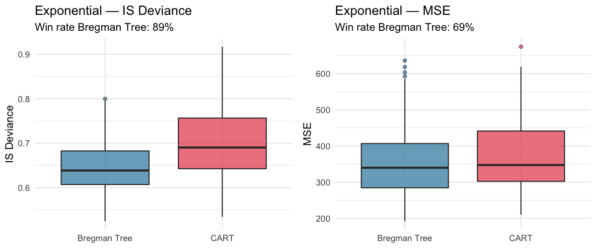
   Under an exponential data generating process, the Bregman Tree outperforms CART-anova on both metrics and in the vast majority of individual replications. The IS deviance advantage is substantial: the Bregman Tree reduces the mean IS deviance relative to CART-anova ($0.6487$ vs. $0.6994$). More strikingly, the Bregman Tree also achieves a lower mean MSE ($359.81$ vs. $374.54$) and wins on MSE in $69\%$ of replications, despite MSE being the criterion that CART-anova directly optimises during training. This suggests that a distributionally appropriate splitting criterion may improve generalisation even on metrics that are not explicitly optimised during training.

   Table 4: Monte Carlo results: Exponential model.

   Model	Mean IS Dev.	Mean MSE	Win rate (IS)	Win rate (MSE)
   Bregman Tree	0.6487	359.8187	89%	69%
   CART-anova	0.6994	374.5418	11%	31%

2. Second Simulation: Gamma model. The Exponential is a special case of the Gamma family, and the IS divergence remains the natural splitting criterion for both. Increasing the shape parameter $\alpha$ reduces the coefficient of variation of the response, making the data less dispersed than in Simulation 1. We generalize the previous simulation by considering a Gamma-distributed response $Y\sim\Gamma(k,\theta)$. The Bregman divergence is still the Itakura-Saito divergence $D_{\phi}(y,\mu)=\frac{y}{\mu}-\log\left(\frac{y}{\mu}\right)-1$

   The data are generated as follows $X_{1},X_{2}\sim\mathcal{U}(0,1)$, $\epsilon\sim\mathcal{N}(0,1)$ and the mean structure is $\mu(X)=\exp(1+X_{1}+2X_{2})$ and response is $Y|X\sim\Gamma(k,\theta),\theta=\mu/k$ with shape parameter $k=5$. For the splitting criterion, we compare CART for regression with the quadratic loss of anova and for the Bregman tree Itakura–Saito divergence.

   Table 5: Monte Carlo results: Gamma model with shape $\alpha=5$.

   Model	Mean IS Dev.	Mean MSE	Win rate (IS)	Win rate (MSE)
   Bregman Tree	0.1273	78.25	92%	58%
   CART-anova	0.1471	79.40	8%	42%

   The Bregman Tree is almost uniformly better under the IS deviance and remains slightly superior under MSE. The mean IS deviance of Bregman Trees is $0.1273$ and for CART $0.1471$, and the mean MSE results are $78.25$ and $79.40$ respectively. The win rate reaches 92% under IS deviance and 58% under MSE, indicating a clear advantage for the Bregman Tree under the distributionally appropriate loss, while the difference in MSE is more modest. The stronger dominance relative to Simulation 1 is consistent with the reduced dispersion of the Gamma ($\alpha=5$) response: with less noise in the data, the alignment between the splitting criterion and the true data generative process becomes more decisive, and the misspecification penalty paid by CART-anova is more clearly reflected in the results.

3. Third Simulation: Inverse Gaussian. The response was generated as $Y\mid\mathbf{X}\sim\mathrm{InvGauss}(\mu,\lambda)$, with $\mu=e^{1+X_{1}+2X_{2}}$ and dispersion parameter $\lambda=5$. The Bregman Tree uses the Inverse Gaussian divergence $D_{\phi}(y,\mu)=(y-\mu)^{2}/(2\mu^{2}y)$, associated with the generator $\phi(\mu)=1/\mu$.

   Table 6: Monte Carlo results: Inverse Gaussian model (100 replications).

   Model	Mean IG Dev.	Mean MSE	Win rate (IG Dev.)	Win rate (MSE)
   Bregman Tree	0.1133	1,689.46	63%	49%
   CART-anova	0.1173	1,698.75	37%	51%

   The Bregman Tree exhibits a modest advantage under the Inverse Gaussian deviance, while both methods perform nearly identically in terms of MSE. The mean IG deviance is reduced to $0.1133$ vs. $0.1173$, and also the mean MSE ($1{,}689.46$ vs. $1{,}698.75$). The Inverse Gaussian distribution has heavier tails and a more complex variance structure than the Gamma, which may reduce the effective advantage of using a correctly specified criterion. The Bregman Tree still exhibits a small but systematic advantage under the Inverse Gaussian deviance, while the two methods remain essentially tied under MSE.

   

   (a) First Simulation: exponential model

   

   (b) Second simulation: Gamma model

   

   (c) Third simulation: Inverse Gaussian model

   Figure 3: Bregman Tree fitted under distributional losses unavailable in rpart: Exponential (left), Gamma $(\alpha=5)$ (centre), and Inverse Gaussian $(\lambda=5)$ (right). Each model uses the Bregman divergence associated with its respective data generating process.

4. Fourth Simulation: Poisson model. We consider a Poisson response variable. The associated convex Legendre conjugate is $\phi(\mu)=\mu\log\mu-\mu$ and the Bregman divergence is $D_{\phi}(y,\mu)=y\log\left(\frac{y}{\mu}\right)-(y-\mu)$

   The data are generated as follows $X_{1},X_{2}\sim\mathcal{U}(0,1)$, $\epsilon\sim\mathcal{N}(0,1)$ and the mean structure is $\mu(X)=\left\{\begin{array}[]{cc}\exp(1+2X_{2})&X_{1}<0.5\\ \exp(2+X_{2})&X_{1}\geq 0.5\end{array}\right.$ with response $Y|X\sim\mathcal{P}(\mu)$.

   In this scenario, both competing methods optimise the same criterion: the Bregman Tree uses the KL divergence $D_{\phi}(y,\mu)=y\log(y/\mu)-y+\mu$, which is exactly the loss minimised natively by the Poisson method implemented in CART. Accordingly, we compare the proposed method with CART using method=’poisson’.

   Table 7: Monte Carlo results: Poisson model (100 replications).

   Model	Mean Dev.	Mean MSE	Win rate (Dev.)	Win rate (MSE)
   Bregman Tree	0.5999	12.6023	43%	38%
   CART-Poisson	0.5900	12.3788	57%	62%

   This simulation serves as a negative control for the study. Since both procedures optimise the same population criterion, no systematic difference should be expected. The empirical results are fully consistent with this prediction. The differences in mean deviance ($0.5999$ vs. $0.5900$) and mean MSE ($12.6023$ vs. $12.3788$) are negligible. The slight edge of CART-Poisson is consistent with random variation rather than a structural difference. This result serves as an important negative control: it confirms that the gains observed in Simulations 1–3 are genuinely attributable to criterion alignment, and not to some incidental implementation advantage of the Bregman Tree.

5. Fifth Simulation: Gaussian model. We finally look at a gaussian response variable. The associated convex Legendre conjugate is $\phi(\mu)=\frac{1}{2}u^{2}$ and the Bregman divergence is the quadratic divergence $D_{\phi}(y,\mu)=\frac{1}{2}(y-\mu)^{2}$. The data are generated as follows

   $X_{1},X_{2}\sim\mathcal{U}(0,1)$, $\epsilon\sim\mathcal{N}(0,1)$ and the mean structure is $\mu(X)=1+X_{1}+2X_{2}$ with response $Y|X\sim\mathcal{N}(\mu(X),1)$

   As in Simulation 4, Bregman Trees and CART-anova optimise the same objective.

   Table 8: Monte Carlo results: Gaussian model (100 replications).

   Model	Mean MSE
   Bregman Tree	1.1301
   CART-anova	1.1229

   Consistent with the Poisson simulation, no meaningful difference is observed between the two methods. The mean MSE values ($1.1301$ vs. $1.1229$) are virtually identical, and the small advantage of CART-anova falls well within the range of Monte Carlo variability. This result closes the logical argument of the simulation study: the Bregman Tree offers no advantage when its splitting criterion coincides with that of the benchmark, and conversely, it provides systematic and sometimes substantial gains when it is strictly better aligned with the true data generating process.

   

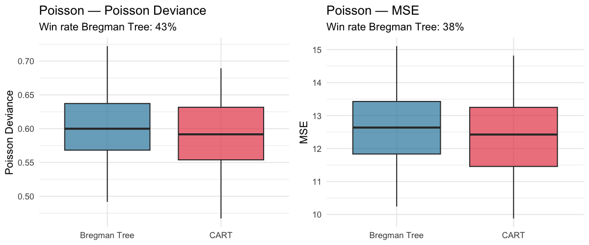
   (a) Poisson model.

   

   (b) Gaussian model.

   Figure 4: Bregman Tree vs. CART under Poisson (left) and Gaussian (right) data generating processes, where both methods optimise the same loss function. No significant differences in predictive performance are observed between the two approaches, confirming that the advantage of the Bregman Trees arises only when its splitting criterion is strictly better aligned with the true distribution than the competing method.

Across all simulations, the advantage of the Bregman Tree appears precisely in settings where the classical CART criterion is misspecified relative to the underlying data generating process. The largest gains are observed for the Exponential and Gamma models, where the Itakura–Saito divergence provides a substantially better match to the conditional distribution than the quadratic loss. For the Inverse Gaussian model the improvement remains present but is more moderate, reflecting the increased variability of the response. In contrast, when both methods optimize the same population criterion, as in the Poisson and Gaussian settings, their predictive performances become essentially indistinguishable. This behaviour is entirely consistent with the theoretical interpretation of split gains as Bregman separations between conditional means and provides empirical support for the proposed framework.

6.1 Real Data set

We conclude by evaluating the proposed method on a real data set. The analysis is based on the insurance dataset, which contains 1,338 records of medical insurance costs in the United States. The response variable charges represents the amount billed to the patient by the insurer, expressed in US dollars It is a continuous variable, strictly positive, and displays a pronounced right-skewed distribution, which is consistent with a Gamma family model, which is well suited for strictly positive, heteroscedastic responses where the variance tends to grow with the mean. The explanatory variables are age, body mass index (BMI), smoking status, number of children, sex, and geographic region.

We fitted three single-tree models and compared them on a 70/30 train-test split. Each model follows the same recursive partitioning logic but differs in the splitting criterion it optimises, which makes the comparison particularly informative about the role of the loss function in the tree-based modelling.

For the Bregman Tree, according to a possible Gamma distribution of $Y$, at each node, the split is chosen so as to minimise the Itakura–Saito (IS) divergence, which is the Bregman divergence naturally associated with the Gamma family through the convex generator $\phi(\mu)=-\log\mu$. Because this criterion is tailored to the distributional assumption of the response, one would expect it to yield better-calibrated predictions under a Gamma model. The final tree was selected by the 1-SE pruning rule. We compare this method with a the classical CART algorithm with anova, which greedily minimises the mean squared error (MSE) at each split. Although MSE is the standard choice for continuous responses, it implicitly assumes homoscedastic errors, an assumption that is unlikely to hold for insurance charges. The tree was pruned also by the 1-SE rule. Last we perform a variant of CART that replaces MSE with the Poisson deviance as the splitting criterion. The Poisson deviance penalises relative rather than absolute errors, making it more robust to the heavy tail of the response. As with the other models, pruning was carried out via the 1-SE rule.

The model performance on the test sample was assessed using three complementary and accord metrics. The IS deviance $\mathrm{IS}(y,\hat{y})=\frac{1}{n}\sum_{i=1}^{n}\left(\frac{y_{i}}{\hat{y}_{i}}-\log\frac{y_{i}}{\hat{y}_{i}}-1\right)$ measures how well predictions align with the Gamma assumption; the Poisson deviance $\mathrm{DevPoisson}(y,\hat{y})=\frac{1}{n}\sum_{i=1}^{n}\left(y_{i}\log\frac{y_{i}}{\hat{y}_{i}}-y_{i}+\hat{y}_{i}\right)$ captures relative prediction accuracy, and finally we compare with the $\mathrm{MSE}(y,\hat{y})=\frac{1}{n}\sum_{i=1}^{n}(y_{i}-\hat{y}_{i})^{2}$.

In Table 9 we summarises the performance of the three models where we can see that the choice of splitting criterion has a meaningful impact on predictive accuracy, particularly when the response distribution departs from normality.

Table 9: Out-of-sample performance of the three tree models on the test set.

Model	Leaves	IS Deviance	Poisson Dev.	MSE
Bregman Tree	22	0.1212	1,895	21,343,132
CART-anova	7	0.1443	2,097	22,314,072
CART-Poisson	27	0.1256	1,861	20,666,475

In terms of tree size, CART-anova produces the most parsimonious structure, with only 7 terminal nodes. While this compactness is appealing from an interpretability standpoint, it comes at a cost: CART-anova yields the worst performance across all three metrics, suggesting that the model is underfitting the data. At the other extreme, CART-Poisson grows the most complex tree with 27 leaves, yet it achieves the lowest MSE ($20{,}666{,}475$) and the best Poisson deviance ($1{,}861$), indicating that the additional splits are capturing genuine structure in the data rather than noise. The Bregman Tree sits between the two, with 22 leaves, and attains the lowest IS deviance ($0.1212$), which is the metric most directly aligned with its training objective and with the assumed Gamma distribution of the response.

Regarding the IS deviance—the metric most relevant under a Gamma model—the Bregman Tree outperforms both CART alternatives, as expected given that its splits are explicitly designed to minimise this criterion. The gap between the Bregman Tree ($0.1212$) and CART-anova ($0.1443$) is notable, representing roughly a $16\%$ relative reduction in IS deviance. CART-Poisson ($0.1256$) closes much of this gap, which is not surprising since the Poisson deviance also penalises relative errors and thus shares structural similarities with the IS divergence.

In terms of MSE, CART-Poisson performs best ($20{,}666{,}475$), followed closely by the Bregman Tree ($21{,}343{,}132$), while CART-anova lags behind ($22{,}314{,}072$). The differences in MSE are substantial in absolute terms—over one million dollars in squared error per observation on average—reflecting the heavy right tail of the charges variable, where a small number of very high-cost cases can drive large squared residuals. The fact that CART-anova, despite optimising MSE directly during training, does not achieve the best test MSE is a reminder that a misspecified training criterion can lead to suboptimal generalisation even on the metric it was designed to minimise.

Taken together, these findings suggest that explicitly accounting for the distributional properties of the response—either through a Gamma-based criterion as in the Bregman Tree, or through a relative-error criterion as in CART-Poisson—leads to better out-of-sample performance than the standard CART based on squared-error loss. The Bregman Tree offers the best balance between IS deviance and model interpretability, while CART-Poisson achieves the lowest absolute and relative prediction errors at the cost of a more complex tree structure.

7 Conclusion

In this work, we introduced a generalization of CART decision trees based on Bregman divergences. This framework extends the classical impurity criterion by replacing the impurity function with a general Bregman divergence adapted to the statistical geometry of the problem.

Our results show that many impurity criteria commonly used in machine learning — including squared loss, logistic deviance, Poisson deviance, and Kullback–Leibler divergence — can be understood within a single unified framework. In particular, the impurity gain associated with a split admits a natural geometric interpretation in terms of Bregman divergences between parent and child node barycenters.

Beyond the algorithmic perspective, the proposed approach establishes a rich connection between decision trees, convex analysis, and information geometry. Properties of the generating convex function, such as strong convexity and smoothness, directly influence the behavior of impurity gains and provide quantitative control on the geometry of the partitioning process.

The numerical experiments support the theoretical findings. When the impurity criterion is aligned with the underlying data-generating process, Bregman trees consistently outperform standard CART procedures. Conversely, when both methods optimise the same population criterion, their performances become essentially indistinguishable. These results suggest several possible directions for future work, including consistency analysis, statistical rates, extensions to classification settings, and the development of ensemble methods based on non-Euclidean impurity criteria. More broadly, Bregman trees provide a flexible framework for adapting decision tree methods to the intrinsic geometry of the underlying statistical model.