Few-Shot Prediction for Pulsar Noise with Long Short-Term Memory Network
Abstract
This work proposes a novel solution to predict pulsar timing residuals with limited data, addressing the critical challenge of data scarcity across spin-frequency subgroups of millisecond pulsars in PTA datasets. The proposed solution applies a Long Short-Term Memory (LSTM) network optimized using the model-agnostic meta-learning algorithm, enabling rapid adaptation to new frequency domain by fine-tuning the LSTM network with only a few-shot of ground truth timing residuals. Particle swarm optimization algorithm is also used for automatic hyperparameter optimization, leading to improved prediction accuracy. Our solution, evaluated on the second data release of the International Pulsar Timing Array (IPTA), demonstrates robust generalization with accurate predictions in three metrics across high-frequency test frequency domains, while requiring only 10% of the timing residuals from these domains for model fine-tuning. Furthermore, our lightweight structure only costs 16.86 MB CPU memory and 18 milliseconds for single-step residual prediction. All these characteristics make our solution highly suitable for real-world applications, where effective and real-time predictions of pulsar timing residuals are essential—particularly in resource-constrained environments with limited computational power, memory, or energy availability.
show]yuqi.ouyang@scu.edu.cn
I Introduction
Pulsar timing is a critical technique for detecting gravitational waves in the nanohertz–microhertz frequency regime by characterizing timing residuals derived from time-of-arrival measurements (TOAs) (Foster et al., 1990; Sazhin, 1978; Detweiler and Szedenits Jr, 1979). It relies on accurate TOAs of pulses from millisecond pulsars, which are recorded with uncertainties arising from instrumental effects and radio frequency interference (RFI) Agazie et al. (2023). Timing residuals, defined as the differences between observed and predicted TOAs, arise due to deviations of the timing model parameters from their true values as well as various noise processes that must be characterized to ensure robust and statistically consistent inference of timing model parameters. These residuals reflect the combined influence of imperfect timing model parameters and stochastic noise processes that perturb pulse arrival times and therefore form the basis for assessing the fidelity of the timing model. A key difficulty is that these contributions can mask or become covariant with astrophysical signals embedded in the TOAs. For instance, perturbations induced by nanohertz gravitational waves from the inspiral and merger of supermassive black holes can be covariant with rotational irregularities, interstellar medium variations, or residual instrumental noise van Haasteren and Levin (2012). Consequently, the accurate prediction of timing residuals establishes a dynamic empirical baseline for pulsar observations. This serves as a vital practical utility for the real-time identification of anomalies, such as unexcised radio frequency interference (RFI), instrumental systematics, or sudden interstellar medium (ISM) events Agazie et al. (2023), prior to the execution of computationally intensive offline analyses such as Gaussian Processes Coles et al. (2011); van Haasteren and Levin (2013). Also, these residuals exhibit structure on timescales determined by stochastic noise processes and long-term timing irregularities. Each pulsar emits pulses at a rate given by its rotation frequency, typically ranging 100 Hz to over 600 Hz for millisecond pulsars and varying across the pulsar timing array population. To enable few-shot domain adaptation within the MAML framework, we partition pulsars into frequency domains based on their spin frequency as a practical grouping strategy. This allows the model meta-trained on well-sampled lower-frequency domains to rapidly adapt to higher-frequency domains with limited observations, thereby improving timing model fidelity and supporting the detection of astrophysical signals such as gravitational waves.
The task of noise modeling has been a challenge in the pulsar timing community, with efforts evolving over decades to refine techniques and address persistent flaws. Initially, Blandford et al. (1984) pioneered basic statistical approaches to characterize timing residuals, laying a foundation for noise subtraction; however, their method had difficulty capturing the the power-law spectrum of red noise, which exhibits stronger power at low Fourier frequencies. Building on this, Manchester et al. (2013) introduced more robust data preparation pipelines, establishing pulsar timescales through high-precision observations, while was still challenged by the complexity of low-frequency noise components. Verbiest et al. (2008) identified pervasive low-frequency timing irregularities, exposing the limitations of prior frameworks and prompting a shift toward more advanced methodologies. Recently, Susobhanan et al. (2024) developed a frequency analysis framework within dedicated software, enabling simultaneous fitting of noise and timing parameters to improve accuracy. In addition to these contributions, Gaussian processes have emerged as a cornerstone of pulsar noise analysis, offering a flexible, non-parametric approach to model both white and red noise components, significantly improving the precision of noise parameter estimation Shannon and Cordes (2010c); Coles et al. (2011); Lentati et al. (2013); van Haasteren and Levin (2013). Furthermore, Kalman filters have recently been adopted as a method for real-time, adaptive noise modeling, particularly effective for handling non-stationary noise processes O’Neill et al. (2024).
While representing a significant advancement, previous approaches remain limited, due to the high computational complexity of standard Gaussian Processes and the rigid parametric assumptions often required to make noise modeling computationally tractable for large datasets (Coles et al., 2011), this underscores the need for innovative approaches. In the new era, deep learning methods have shown excellent capability in data modeling and analysis Hochreiter and Schmidhuber (1997); Ismail Fawaz et al. (2020); Goodfellow et al. (2014); Ho et al. (2020). In particular, the Long Short-Term Memory networks (LSTMs), introduced by Hochreiter and Schmidhuber (1997), excel in predictive modeling tasks by capturing long-term dependencies within sequential data Lorenzo et al. (2017). This makes LSTMs ideal for pulsar timing, where temporal correlations arising from all stochastic contributions to the timing residuals, including achromatic red noise from spin irregularities, chromatic ISM effects, and instrumental noise, allow for sequential prediction, aligning closely with our task of modeling the total residuals. However, despite the suitability of LSTM networks for the prediction task, two challenges still remain: data scarcity and hyperparameter optimization of the deep learning models. While radio telescopes provide pulsar observations, data scarcity exists for newly discovered or high-frequency MSPs due to limited telescope time and instrumental constraints Wang (2023); Lynch et al. (2018); Perera et al. (2019). Deep learning models, which are based on large labeled datasets, typically suffer from data scarcity Liu et al. (2024). To address this, a few-shot learning strategy is proposed. In this strategy, pulsars are first grouped into domains based on spinning frequencies. A prediction model is then trained on well-represented domains and adapted to data-scarce ones. This can be achieved using model-agnostic meta-learning (MAML), an optimization algorithm compatible with any gradient-based deep learning model, enabling rapid adaptation with minimal data Finn et al. (2017). As for the challenge of hyperparameter optimization, traditional grid search in deep learning models is often costly, time-consuming, and requires human supervision. To improve efficiency, the Particle Swarm Optimization (PSO) algorithm Jain et al. (2022) is incorporated to automate hyperparameter tuning, enhancing prediction accuracy and model robustness.
Prior to this work, the standard noise modeling method using Gaussian processes van Haasteren and Vallisneri (2014), here we summarize the qualitative comparison between the two approaches: The Gaussian-process (GP) framework commonly used in pulsar-timing noise analysis models timing residuals as sums of stochastic processes whose covariance functions encode physically motivated priors (e.g., power-law red noise, frequency-dependent DM, and inter-pulsar Hellings–Downs correlations). This yields principled marginalization, component separation and predictive uncertainty quantification that are particularly useful for detection or attribution tasks. However, its original form incurs scaling in the number of TOAs, practical PTA analyses therefore rely on low-rank or Fourier expansions and specialized samplers to make full-noise Bayesian inference tractable. GP methods are for the situation when principled uncertainties and physical component separation are required (for example, in gravitational-wave searches searches). By contrast, our approach is fully data-driven and predicatively few-shot: we meta-train a bidirectional LSTM on uniformly resampled (1-day grid) residual sequences across well-sampled frequency domains, and fine-tune with only a small fraction (10%) of data from a target domain. Additionally, PSO is incorporated for automatic hyperparameter selection. These enable our model to capture potentially nonlinear and nonstationary structures without prescribing a covariance family, while producing fast, lightweight single-step predictions once meta-trained (16.9 MB and 18 ms per step in our tests). Compared with GP framework, our solution excels when fast and accurate few-shot predictive performance and low computational footprint are the priority. To sum up:
This work proposes a novel solution to address the data scarcity challenge in pulsar noise analysis. First, MAML is applied for few-shot learning, where the model is first trained with multiple pulsars across low-frequency domains categorized by spinning frequencies, and then fine-tuned with a limited amount of data from a targeted high-frequency domain, achieving domain adaptation with accurate prediction results. Furthermore, the PSO algorithm is utilized to provide an automated solution for hyperparameter optimization, further enhancing the prediction performance. The main contributions of this work are summarized as follows:

sequence; is the next-step output of timing residual with denoting network parameters; is cell input; , , denote the output of the forget gate, input gate, output gate, respectively; , are the cell states; , are the hidden states.
-
1)
Our work addresses the data scarcity issue in pulsar noise analysis, achieving accurate predictions across multiple frequency domains in the second data release of the International Pulsar Timing Array (IPTA) Antoniadis et al. (2022), while requiring only a few data from the targeted frequency domains.
-
2)
A fully automated solution is provided with automatic hyperparameter optimization, leading to further enhanced prediction accuracy and model robustness.
-
3)
Real-time efficiency is achieved with a lightweight model, requiring only 16.9 MB of CPU memory for an inference speed of 18 milliseconds. Our prediction accuracy, efficiency, and generalizability make our solution well suited for real-world applications. Comprehensive experimental analysis is presented to validate our core functionalities.
The remainder of this paper is organized as follows. In Section II, we present our proposed solution, detailing the bidirectional LSTM architecture, the application of the MAML framework for few‐shot domain adaptation, and the integration of the PSO algorithm for automatic hyperparameter tuning. Section III describes the experimental setup, including the IPTA DR2 dataset, implementation details, evaluation metrics, and comprehensive performance results across multiple test domains.
II Methods
In this work, unless otherwise specified, references to frequency domains denote groups of pulsars categorized by their rotational frequencies as a practical partitioning strategy for MAML domain adaptation on the IPTA DR2 MSP ensemble. This is distinct from radio observing frequencies (MHz-GHz) and Fourier frequencies (nHz).
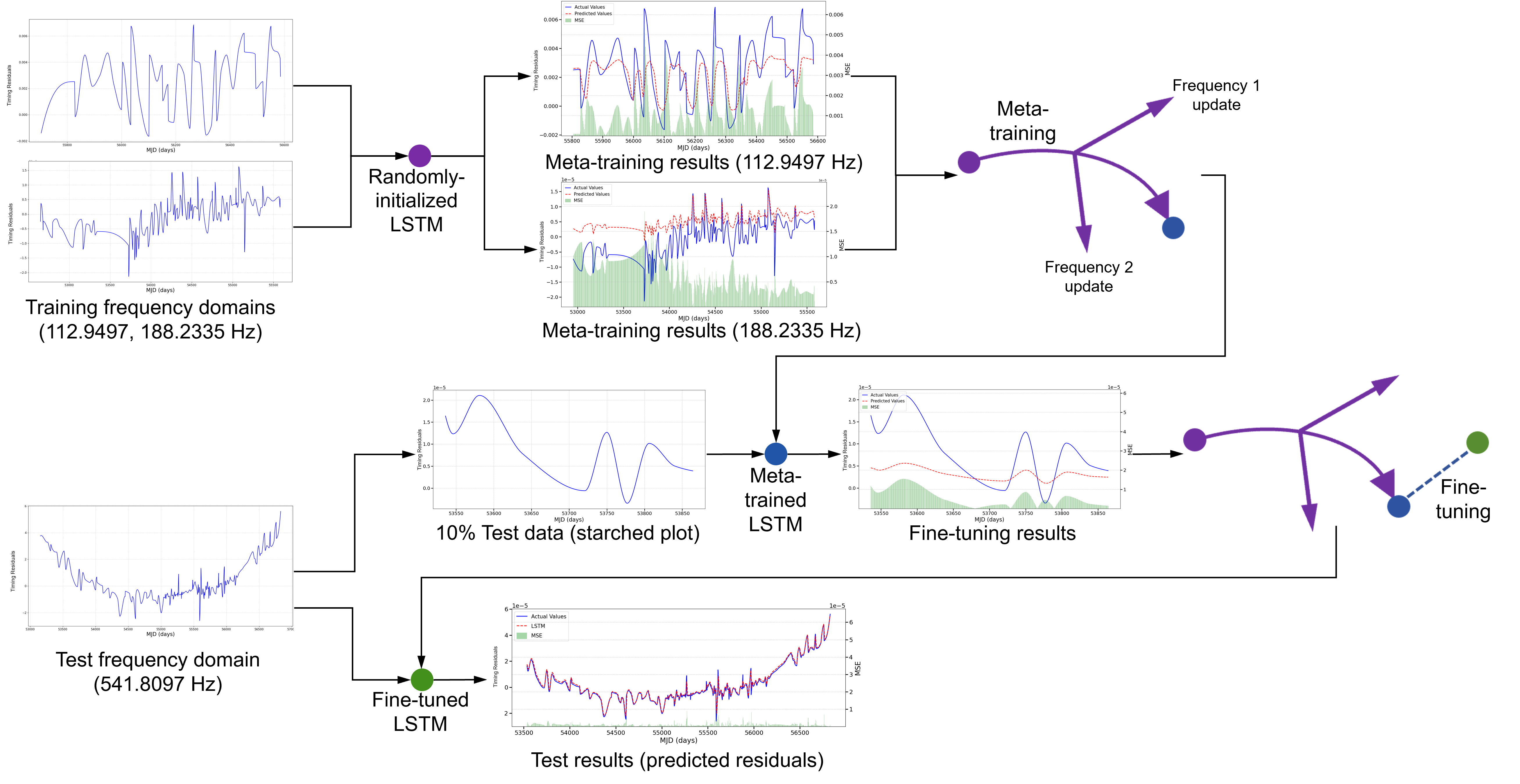
Depicted in Figure 1, our solution includes three processes: meta-training, fine-tuning, and testing. In meta-training, timing residuals from low-frequency domains (112.9497 Hz and 188.2335 Hz) are used to form cross-frequency prediction tasks, leading to a coarse LSTM initialization named meta-trained LSTM, which is further updated in the fine-tuning stage with only a few timing residuals from an unseen high frequency domain (10%, 541.8097 Hz in our example), performing fast and accurate domain adaptation in a few-shot setting.
LSTM selectively retains or discards information through a gate system in its cell structure, effectively addressing the gradient vanishing and exploding issues often encountered when processing long sequences Graves and Graves (2012). Bidirectional LSTMs capture temporal dependencies in both forward and backward directions, allowing for improved integration of contextual information and more accurate modeling of temporal patterns in sequential data Zhou et al. (2016); Zhang et al. (2015). Based on this, our prediction task, as depicted in Figure 2, starts from a bidirectional LSTM processing the historical timing residual sequence which represents resampled timing residuals. Since original pulsar observations are recorded at irregular intervals, we apply linear interpolation to map the observed residuals onto a uniform grid with a constant 1-day interval in Modified Julian Date (MJD). This sequence, processed with a window size of steps, is followed by concatenating the bidirectional hidden states, and mapping the concatenation through fully-connected layers to predict the next-step timing residual , with denoting the forward computing process using trainable parameter set . The timestep interval is one day of MJD.
II.1 The LSTM Cell
In Figure 2, the LSTM layer contains multiple cells with common neural structure depicted for pattern analysis, highlighting the gate system that controls the flow of information. Such a gate system consists of three main components: the forget gate, the input gate and the output gate, explained next.
The forget gate decides information discarding from the cell state, presented as:
| (1) |
where is the weight matrix, is the bias, is the input vector at time step , is the previous hidden state, and denotes the Sigmoid function. Thus, is a gating vector with real numbers bounded in , determining the proportion of information to forget at each unit.
The input gate determines information addition to the cell state, as follows:
| (2) |
| (3) |
where and are the weight matrices; and are the bias terms; denotes the hyperbolic tangent function. Therefore, is the input gate vector with real numbers bounded in , and is the candidate cell state vector with values bounded in .
The cell state is computed as a weighted addition between the previous cell state and the candidate cell state:
| (4) |
where is the previous cell state. integrates both the retained and updated information.
In the end, the output gate computes the hidden state based on the cell state , as follows:
| (5) |
| (6) |
where is the weight matrix, is the bias, the hidden state is with real numbers bounded in . The design of gate system enables LSTM to extract and maintain long-term dependencies from time-series data.
II.2 Model-Agnostic Meta-Learning
Figure 3 depicts a demonstration of our MAML learning strategy. Based on parameter optimizations on multiple frequency domains, the meta-training process searches for a model initialization as a prior knowledge. Hence, instead of training from the ground for new frequencies, fast adaptation is enabled to each new frequency domain in fine-tuning process, such few-shot strategy addresses data scarcity issue through domain adaptation. All optimizations in the MAML strategy are based on gradient descent guided by mean squared error (MSE) loss computed from the residual prediction tasks, denoted as follows:
| (7) |
where denotes that the the input and the ground truth timing residuals are sampled from the dataset of the frequency domain; computes the norm; denotes to the sample size.
The meta-training stage consists of residual prediction tasks from multiple frequency domains, adopting a nested optimization to learn an LSTM initialization, mathematically formulated as follows:
| (8) |
| (9) |
where and are learning rates for the inner optimization and outer optimization, respectively; the subscript denotes the step number of inner gradient descent, where indicates the LSTM initialization. Equation 9 shows that optimizing the LSTM initialization in the outer loop depends on the resulted from the inner loop. Hence, gradient descent of the outer optimization requires computing the Hessian at the inner optimization, triggering the improved gradient and therefore facilitates fast model adaptation on new data domains. Note that to implement the nested optimization, data samples from each training frequency domain are partitioned into two sets for the inner and outer parts, respectively.

After meta-training, the fine-tuning process rapidly adapts the learned initialization to new frequency domains, as depicted by the blue dashed lines in Figure 3. Such adaptation runs with a small number of gradient steps, calculated from the prediction tasks associated with limited data from each test frequency domain.
II.3 Particle Swarm Optimization
In our solution, the PSO algorithm finds optimal hyperparameters that leads to the minimal loss value. To achieve this, the algorithm regards these hyperparameters as particle locations, then initiates and iteratively updates multiple particles’ velocity and location, respectively as follows:
| (10) |
| (11) |
where denotes particle velocity; means particle location; subscript is for the PSO iteration number; subscript defines current optimal locations with minimal loss, while and respectively denote particle’s optimal location and the whole swarm’s global optimal location, dynamically renewed with the ones associated with lower loss values; is the inertia weight; and are the learning factors; , are random numbers that ensures searching diversity.
In Equation 10, the velocity, i.e., the moving direction of each particle is computed based on the personal optima and the shared information of the global optima , reflecting the natural swarm behavior of information sharing while exploring for resources. By covering a wide search space, such swam optimization strategy helps escape local minima, leading to more robust result Wang et al. (2018). Following the iterative process, the PSO algorithm provides an automatic solution for hyperparameter setting. In this work, the PSO algorithm is applied to search for three key hyperparameters for the meta-training process: learning rate and gradient descent iteration number in the inner-optimization, and the learning rate in the outer-optimization.
II.4 Comparison with Standard Noise Modeling Methods
The Gaussian-process (GP) framework van Haasteren & Vallisneri (2014) commonly used in pulsar-timing noise analysis models timing residuals as sums of stochastic processes whose covariance functions encode physically motivated priors (e.g., power-law red noise, frequency-dependent DM, and inter-pulsar Hellings–Downs correlations). This yields principled marginalization, component separation and predictive uncertainty quantification that are particularly useful for detection or attribution tasks. However, its original form incurs scaling in the number of TOAs, practical PTA analyses therefore rely on low-rank or Fourier expansions and specialized samplers to make full-noise Bayesian inference tractable. GP methods are for the situation when principled uncertainties and physical component separation are required (for example, in gravitational-wave searches searches).
By contrast, our approach is fully data-driven and predicatively few-shot: we meta-train a bidirectional LSTM on uniformly resampled (1-day grid) residual sequences across well-sampled frequency domains, and fine-tune with only a small fraction (10%) of data from a target domain. Additionally, particle swarm optimization (PSO) is incorporated for automatic hyperparameter selection. These enable our model to capture potentially nonlinear and nonstationary structures without prescribing a covariance family, while producing fast, lightweight single-step predictions once meta-trained (16.9 MB and 18 ms per step in our tests). Compared with GP framework, our solution excels when fast and accurate few-shot predictive performance and low computational footprint are the priority.
III Experiment
III.1 Dataset
In this work, version B of IPTA DR2 dataset Verbiest et al. (2016) is used. In the dataset, long-term, high-precision pulsar timing observations from three constituent PTAs are integrated to enhance temporal diversity and global spatial coverage for improved sensitivity to nanohertz gravitational wave signals. The three PTAs are: the European Pulsar Timing Array (EPTA) Antoniadis et al. (2023), the North American Nanohertz Observatory for Gravitational Waves (NANOGrav) Arzoumanian et al. (2015), and the Parkes Pulsar Timing Array (PPTA) Zhu (2024). More specifically, the IPTA DR2 dataset includes timing observations from 49 millisecond pulsars (MSPs), which exhibit red noise characteristics. The data span a temporal baseline of up to 24 years, with MJD values ranging from 46436 (1986 January 06) to 56598 (2013 November 02), based on the earliest observations recorded in Kaspi et al. (1994) and the latest in Zhu et al. (2015). The selected MSPs, characterized by rapid rotation, have spin frequencies ranging from 62.3 Hz to 641.8 Hz Verbiest et al. (2016). Low-frequency noise is dominated by long-term trends and interstellar medium effects, resulting in higher amplitude but smoother variations Lentati et al. (2016). Comparatively, high-frequency noise is more challenging to model due to the variance caused by instrumental and short-term astrophysical effects Shannon and Cordes (2010b); Shannon et al. (2014), forming the primary focus of domain adaptation for modeling timing residuals in our work.
III.2 Implementation Details
The timing residuals, as the difference between the actual TOA and the predicted TOA based on the timing model Píriz et al. (2019); Zhang et al. (2024), are linearly rescaled to the range in this work. The bidirectional LSTM in our solution are designed with two stacked layers and a hidden size 200. To mitigate overfitting, dropout with rate 0.2 is applied on LSTM and LSTM output. In the end, fully connected layers are used to produce the output, the layer-wise neurons numbers are 100 and 1, with the first layer activated with ReLU function.
Pulsar timing residual sequences in the PTA sample exhibit variations across the observed range of spin frequencies, which we use to define domains for cross-pulsar adaptation Parthasarathy et al. (2019); Shannon and Cordes (2010a). To demonstrate our adaptation ability, we design the training on two low-frequency domains of 112.950 Hz and 188.234 Hz, while the fine-tuning and evaluations are set on three high-frequency domains of 607.670 Hz, 541.810 Hz, and 420.189 Hz. During meta-training, the LSTM network is optimized for 100 epochs, with timing residuals from each frequency domain divided into for inner optimization with learning rate , and for outer optimization with learning rate . The PSO algorithm is applied to set learning rate and gradient descent iteration number in the inner-optimization, and the learning rate in the outer-optimization as , and , ranging between and , and , as well as and , respectively. 5 particles are initialized with a maximum iteration 10. The inertia weight of the PSO optimizer is set to 0.9. The two learning factors for social and individual components are configured as 0.5 and 0.3 respectively. For each test frequency domain, the first timing residuals is used for fine-tuning, while the remaining is for performance evaluation. Adam Sun (2020) optimizers with the default setting are applied for all learning tasks.

III.3 Evaluation Metrics
Various metrics are applied to evaluate and compare model performance, they are: mean absolute error (MAE), mean squared error (MSE), mean absolute percentage error (MAPE), and coefficient of determination (), calculations are respectively defined as follows:
| (12) |
| (13) |
| (14) |
| (15) |
where denotes that the residual sequence and the ground truth is sampled from the frequency domain. More accurate predictions are those with lower MAE, lower MAPE, or higher values.
III.4 Overall Performance
The prediction results on three test frequencies are tabulated in Table 1, overall depicting high values. Especially the 0.9933 value at test frequency 541.810 Hz. Note that our solution is only fine-tuned with of the data from these large frequency domains. These findings indicate that the our solution can address the data scarcity issue with accurate prediction results. However, the functionalities of model components require further studies to validate, presented in the following sections.
| Frequency (Hz) | metrics | ||
|---|---|---|---|
| MAE(%) | MAPE | ||
| 420.189 | 0.2736 | 0.9828 | |
| 541.810 | 0.0001 | 0.2021 | 0.9933 |
| 607.678 | 0.0002 | 0.4210 | 0.9520 |
III.5 Comparative Study of MAML
To study the effect of our few-shot strategy, we compare MAML with mixed training and transfer learning strategies. In mixed training, the model is trained by combining the low-frequency training data with the 10% high-frequency test data, while in transfer learning, the model is first trained with the training set and subsequently fine-tuned using the same 10% test data. The prediction results are summarized in Table 2, demonstrating that MAML achieves more accurate prediction results across all three test frequency domains, exhibiting lower MAE, lower MAPE, and higher values. Notably, at 420.189 Hz, MAML reduces the MAP from 0.0006% from transfer learning to 0.0001%, while significantly improving from -0.4155 to 0.9019. At 541.810 Hz, MAML maintains the lowest MAPE of 0.8069, substaintially reducing those achieved by mixed Training and Transfer Learning. At 607.678 Hz, MAML achieves an value of 0.8753, outperforming the 0.6708 attained by mixed training and 0.3545 achieved via transfer learning. These results conclusively show that conventional training strategies suffer from data scarcity, while the proposed few-shot MAML strategy addresses this issue with improved model generalization.


| Setting | Frequency (Hz) | ||
|---|---|---|---|
| 420.189 | 541.810 | 607.678 | |
| Mixed Training | 0.0004|1.0175|0.4241 | 0.0008|1.5254|0.3374 | 0.0006|0.5976|0.6708 |
| Transfer Learning | 0.0006|3.4075|-0.4155 | 0.0008|2.4771|0.5551 | 0.0008|1.5336|0.3545 |
| MAML | 0.0001|1.1780|0.9019 | 0.0002|0.8069|0.9789 | 0.0004|0.9602|0.8753 |
| Setting | Frequency (Hz) | ||
|---|---|---|---|
| 420.189 | 541.810 | 607.678 | |
| MAML | 0.0001|1.1780|0.9019 | 0.0002|0.8069|0.9789 | 0.0004|0.9602|0.8753 |
| PSO-MAML | |0.2792|0.9820 | 0.0001|0.2021|0.9933 | 0.0002|0.4210|0.9520 |
The prediction results at test frequency 541.810 Hz, computed from these three settings, are further depicted in Figure 4, where curves are used to demonstrate the residual predictions and the ground truth, bar chart are for MSE values illustrating the divergence. From Figure 4, timing residuals predicted by MAML (black curve) effectively captures the dynamics of the ground truth data (blue curve), while the predictions produced by mixed training (green curve) or transfer learning (orange curve) largely deviates from the real values, visualized from the bar chart. These findings demonstrate the strong adaptability of the MAML learning strategy over the learning incompetence with limited data.
III.6 Evaluating The PSO
Our solution integrates the PSO algorithm for automatic hyperparameter optimization. To further study the effect of the PSO algorithm, performance on the three test frequency domains are tabulated in Table 3, showing consistent prediction improvements across all frequency domains with the integration of PSO. For example, the application of PSO achieves 0.2021 MAPE at test frequency 541.810, comparatively lower than the 0.8069 produced without the PSO. Also applying the PSO algorithm leads to increased values across all three test frequencies, such improved capture of systematic data variations validates the PSO’s effectiveness.
For further investigation, the prediction results on test frequency 541.810 Hz are illustrated in Figure 5, where the prediction results with the PSO algorithm (red curve) align more closely with the actual residuals (blue curve), fitting both overall trends and local fluctuations more accurately than those produced without the PSO, i.e., MAML solely (black curve).


III.7 K-Shot Analysis
In few-shot learning, the shot number is an important setting that defines the proportion of data used in the MAML’s fine-tuning process. In this study, three shot percentiles 5%, 10%, and 20% are selected to fine-tune our meta-trained LSTM, while the last 80% data is used for evaluation to ensure fair comparisons across the three shot settings. Table 4 tabulates the performance with the three shot numbers at test frequency 420.189 Hz, demonstrating that increasing the fine-tuning data from 5% to 20% generally improves prediction results across all three metrics. For instance, the MAE decreases from 0.000007% to 0.000005%, while the MAPE declines from 0.3107 to 0.2736. As for the , such value rises to when fine-tuning with 20% data.
| Shot-number (%) | metrics | ||
|---|---|---|---|
| MAE(%) | MAPE | ||
| 5 | 0.000007 | 0.3107 | 0.9781 |
| 10 | 0.000005 | 0.2792 | 0.9820 |
| 20 | 0.000005 | 0.2736 | 0.9828 |
In Figure 6, prediction curves at test frequency 420.189 Hz, computed by varying the three shot settings, are depicted to provide additional insights. With 5% fine-tuning data, the predicted residuals (red curve) deviates from the actual values (blue curve) between MJD 56200 and 56300, suggesting potential underfitting in fine-tuning. As for the 10% and 20% settings, the predictions align well with real values and the errors are relatively lower, providing more robust predictions. Despite the best predictions are attained at the 20% case, we select 10% for fine-tuning due to the marginal performance difference between these two settings, while the lower proportion of 10% aligns more closely with our objective of addressing the data scarcity issue. These findings validate our accurate predictions with limited data, also providing valuable insights regarding the proportion of data for fine-tuning the model.
III.8 Computational Efficiency
Our solution only contains 13.3M trainable parameters. All the experiments are performed using PyTorch 2.2.1 on a laptop with a 12th Gen Intel Core i9-12900H CPU. Training consumes around 7895.8 MB CPU memory, while single-step residual prediction only costs 16.9 MB CPU memory in 18.0 milliseconds (around 55.5 sample-per-second). The low memory consumption and rapid inference largely improve the practicability, enabling real-time pulsar residual prediction on real-world pulsar observation systems constrained with limited computational resources.
IV Conclusion
This work introduces a novel solution for few-shot prediction of pulsar timing residuals, addressing the challenges of data scarcity and model adaptability across domains. Our solution uses an LSTM network optimized with the MAML learning strategy to learn a generalized parameter initialization from low-frequecy domains, enabling rapid and accurate fine-tuning based on limited data from each high-frequency domain. The integration of the PSO algorithm automatically optimizes hyperparameters and therefore makes our solution fully automated with improved prediction results. Key findings from evaluations and experimental analysis on the IPTA dataset are summarized as follows:
-
1)
Robust generalization. Our solution demonstrates strong adaptability by enabling neural networks with recurrent layers to operate in data-scarcity scenarios across diverse frequency domains, outperforming traditional transfer learning strategy with reduced errors up to 67.42% MAPE (e.g., from 2.4771 to 0.8069 on 541.810 Hz).
-
2)
Accurate predictions. Our solution demonstrates accurate prediction results across all tested high-frequency domains, by requiring only 10% of ground truth data for fine-tuning the model. For example, at the frequency of 541.810 Hz, the solution achieves an MAE of just 0.0001% and an value of 0.9933, demonstrating high precision.
-
3)
Automated solution. The integration of the PSO algorithm enables fully automated optimization of model hyperparameters, allowing the LSTM network to adapt more efficiently to new frequency domains, ensuring rapid and accurate fine-tuning with minimal manual intervention.
-
4)
Exceptional efficiency. Our lightweight structure only consists of 13.3M trainable parameters, requiring only 16.86 MB and 18.0 milliseconds for single-step prediction, making it suitable for real-world applications requiring effective and real-time predictions of pulsar timing residuals in resource-constrained environments.
In conclusion, our work offers an accurate, efficient, and highly adaptable solution for the predictions of pulsar timing residuals in cross-frequency domains, particularly practical in real-world settings. Future research will focus on developing advanced learning strategies to improve predictions in challenging scenarios such as timing noise with weak regularity, therefore further improving our robustness and reliability.
References
- The nanograv 15 yr data set: observations and timing of 68 millisecond pulsars. The Astrophysical Journal Letters 951 (1), pp. L9. Cited by: §I.
- The second data release from the european pulsar timing array: the dataset and timing analysis. Astronomy & Astrophysics 678, pp. A48. Cited by: §III.1.
- The international pulsar timing array second data release: search for an isotropic gravitational wave background. Monthly Notices of the Royal Astronomical Society 510 (4), pp. 4873–4887. Cited by: item 1).
- The nanograv nine-year data set: observations, arrival time measurements, and analysis of 37 millisecond pulsars. The Astrophysical Journal 813 (1), pp. 65. Cited by: §III.1.
- Arrival-time analysis for a millisecond pulsar. Journal of Astrophysics and Astronomy 5, pp. 369–388. Cited by: §I.
- Pulsar timing analysis in the presence of correlated noise. Monthly Notices of the Royal Astronomical Society 418 (1), pp. 561–570. Cited by: §I, §I, §I.
- Black holes and gravitational waves. ii-trajectories plunging into a nonrotating hole. Astrophysical Journal, Part 1, vol. 231, July 1, 1979, p. 211-218. 231, pp. 211–218. Cited by: §I.
- Model-agnostic meta-learning for fast adaptation of deep networks. In International conference on machine learning, pp. 1126–1135. Cited by: §I.
- Timing properties of psr 1951+ 32 in the ctb 80 supernova remnant. Astrophysical Journal, Part 1 (ISSN 0004-637X), vol. 356, June 10, 1990, p. 243-249. 356, pp. 243–249. Cited by: §I.
- Generative adversarial nets. Advances in neural information processing systems 27. Cited by: §I.
- Long short-term memory. Supervised sequence labelling with recurrent neural networks, pp. 37–45. Cited by: §II.
- Denoising diffusion probabilistic models. Advances in neural information processing systems 33, pp. 6840–6851. Cited by: §I.
- Long short-term memory. Neural Computation 9 (8), pp. 1735–1780. Cited by: §I.
- Inceptiontime: finding alexnet for time series classification. Data Mining and Knowledge Discovery 34 (6), pp. 1936–1962. Cited by: §I.
- An overview of variants and advancements of pso algorithm. Applied Sciences 12 (17). External Links: Link, ISSN 2076-3417 Cited by: §I.
- High-Precision Timing of Millisecond Pulsars. III. Long-Term Monitoring of PSRs B1855+09 and B1937+21. ApJ 428, pp. 713. External Links: Document Cited by: §III.1.
- Hyper-efficient model-independent bayesian method for the analysis of pulsar timing data. Physical Review D—Particles, Fields, Gravitation, and Cosmology 87 (10), pp. 104021. Cited by: §I.
- From spin noise to systematics: stochastic processes in the first international pulsar timing array data release. Monthly Notices of the Royal Astronomical Society 458 (2), pp. 2161–2187. Cited by: §III.1.
- Enhancing pulsar candidate identification with self-tuning pseudolabeling semisupervised learning. The Astrophysical Journal 967 (2), pp. 155. Cited by: §I.
- Particle swarm optimization for hyper-parameter selection in deep neural networks. In Proceedings of the genetic and evolutionary computation conference, pp. 481–488. Cited by: §I.
- The green bank north celestial cap pulsar survey. iii. 45 new pulsar timing solutions. The Astrophysical Journal 859 (2), pp. 93. External Links: Document, Link Cited by: §I.
- The parkes pulsar timing array project. Publications of the Astronomical Society of Australia 30, pp. e017. Cited by: §I.
- Analysing radio pulsar timing noise with a kalman filter: a demonstration involving psr j1359- 6038. Monthly Notices of the Royal Astronomical Society 530 (4), pp. 4648–4664. Cited by: §I.
- Timing of young radio pulsars–i. timing noise, periodic modulation, and proper motion. Monthly Notices of the Royal Astronomical Society 489 (3), pp. 3810–3826. Cited by: §III.2.
- The international pulsar timing array: second data release. Monthly Notices of the Royal Astronomical Society 490 (4), pp. 4666–4687. External Links: ISSN 0035-8711, Document, Link Cited by: §I.
- PulChron: a pulsar time scale demonstration for pnt systems. In Proceedings of the 50th annual precise time and time interval systems and applications meeting, pp. 191–205. Cited by: §III.2.
- Opportunities for detecting ultralong gravitational waves. Sov. Astron 22, pp. 36–38. Cited by: §I.
- Assessing the role of spin noise in the precision timing of millisecond pulsars. The Astrophysical Journal 725 (2), pp. 1607. Cited by: §III.2.
- Assessing the role of spin noise in the precision timing of millisecond pulsars. The Astrophysical Journal 725 (2), pp. 1607. Cited by: §III.1.
- Assessing the role of spin noise in the precision timing of millisecond pulsars. The Astrophysical Journal 725 (2), pp. 1607. Cited by: §I.
- Limitations in timing precision due to single-pulse shape variability in millisecond pulsars. Monthly Notices of the Royal Astronomical Society 443 (2), pp. 1463–1481. Cited by: §III.1.
- Optimization for deep learning: an overview. Journal of the Operations Research Society of China 8, pp. 249–294. External Links: Document Cited by: §III.2.
- PINT: maximum-likelihood estimation of pulsar timing noise parameters. The Astrophysical Journal 971 (2), pp. 150. Cited by: §I.
- Understanding and analysing time-correlated stochastic signals in pulsar timing. Monthly Notices of the Royal Astronomical Society 428 (2), pp. 1147–1159. External Links: ISSN 0035-8711, Link, Document Cited by: §I.
- Understanding and analysing time-correlated stochastic signals in pulsar timing. Monthly Notices of the Royal Astronomical Society 428 (2), pp. 1147–1159. Cited by: §I, §I.
- New advances in the gaussian-process approach to pulsar-timing data analysis. Physical Review D 90 (10), pp. 104012. Cited by: §I.
- Precision timing of psr j0437–4715: an accurate pulsar distance, a high pulsar mass, and a limit on the variation of newton’s gravitational constant. The Astrophysical Journal 679 (1), pp. 675. Cited by: §I.
- The international pulsar timing array: first data release. Monthly Notices of the Royal Astronomical Society 458 (2), pp. 1267–1288. Cited by: §III.1.
- Particle swarm optimization algorithm: an overview. Soft computing 22 (2), pp. 387–408. Cited by: §II.3.
- Research progress on x-ray pulsar navigation detectors. Applied Physics 13, pp. 407. External Links: Document Cited by: §I.
- Bidirectional long short-term memory networks for relation classification. In Proceedings of the 29th Pacific Asia conference on language, information and computation, pp. 73–78. Cited by: §II.
- An improved wiener filtration method for constructing the ensemble pulsar timescale. The Astrophysical Journal 962 (1), pp. 2. Cited by: §III.2.
- Attention-based bidirectional long short-term memory networks for relation classification. In Proceedings of the 54th annual meeting of the association for computational linguistics (volume 2: Short papers), pp. 207–212. Cited by: §II.
- Testing theories of gravitation using 21-year timing of pulsar binary j1713+ 0747. The Astrophysical Journal 809 (1), pp. 41. Cited by: §III.1.
- The parkes pulsar timing array. Physics (China) 53 (8), pp. 525–531 (Chinese). Cited by: §III.1.