We study the renormalization group flow of non-local form factors in four-dimensional quantum gravity within the proper-time formalism at quadratic order in the curvature expansion. We show that the flow equations can be integrated down to $k=0$, allowing the reconstruction of the full momentum dependence of the form factors. Within this framework, we construct asymptotically safe solutions at this order. We find that asymptotic safety of the flow does not automatically ensure a finite cutoff-independent $\Lambda\to\infty$ limit for the integrated solutions, which in general develop a logarithmic divergence $\ln(q^{2}/\Lambda^{2})$, so that a renormalization condition is still required. A finite $\Lambda\to\infty$ limit compatible with asymptotic safety is obtained only when the ultraviolet boundary condition selects the non-Gaussian fixed point. This yields finite dimensionful form factors, removes UV logarithmic contributions, and ensures independence from the renormalization scale $\mu$. The resulting renormalized asymptotically safe form factors display a power-law decay $\sim 1/q^{2}$ in the ultraviolet and reproduce the expected logarithmic structure in the infrared, with the Planck scale replacing the renormalization scale.

Asymptotically Safe Gravitational Form Factors from the Proper-Time Flow Equation

I  Introduction

Perturbative quantum gravity based on the Einstein–Hilbert action is not renormalizable beyond one loop. Several approaches have been developed to address this problem. Among them, the asymptotic safety scenario [55, 24, 92, 106, 54, 103, 104, 110, 107] has received considerable attention. Originally proposed by Weinberg, it is based on the existence of a non-trivial ultraviolet fixed point of the renormalization group flow, which can be explicitly identified in $d=2+\epsilon$ dimensions. This observation has motivated extensive studies in four dimensions, primarily within the functional renormalization group framework based on the Wetterich equation [91, 115, 56]. Within this approach, a non-trivial UV-attractive fixed point has been found in a wide range of truncations, starting from the Einstein–Hilbert action and its extensions including higher-order polynomial expansions up to $R^{34}$ [88, 41, 58, 61, 59, 40, 3, 97, 96, 62, 94, 71, 93, 63, 69, 57, 112, 10, 32, 94, 95]. More general truncations involving invariants such as $f(R_{\mu\nu}R^{\mu\nu})$ and $f(R_{\alpha\beta\mu\nu}R^{\alpha\beta\mu\nu})$ have been also considered and provide further evidence for the existence of such a fixed point [60]. Evidence for a UV-attractive fixed point has also been obtained in complementary approaches, including the inclusion of the Goroff–Sagnotti two-loop counterterm [72] and lattice formulations of quantum gravity [6, 86, 5, 45, 85, 7, 87, 4, 17].

The asymptotic safety scenario aims at providing a UV-complete description of gravity by connecting a non-trivial fixed point in the ultraviolet with the infrared regime at $k=0$. However, truncations of the effective action based on a finite number of local curvature invariants inevitably miss part of the physical content of the theory, since quantum corrections generically induce non-local interactions [51, 50, 75, 2, 38]. This feature already appears at quadratic order in the curvature, where one-loop effects generate logarithmic contributions to the effective action of the form $\sim R+R\ln(-\Box/\mu^{2})R+R_{\mu\nu}\ln(-\Box/\mu^{2})R^{\mu\nu}$ [1, 50]. In a UV-complete theory, these infrared logarithmic structures are not expected to remain valid at arbitrarily high energies. Rather, they should emerge as the low-energy limit of form factors encoding the non-perturbative dynamics of the UV regime. Such form factors are expected to remain regular in the ultraviolet and to avoid uncontrolled divergences at trans-Planckian scales. In this description, the explicit dependence on the renormalization scale by $\Box/\mu^{2}$ is replaced by a regular dependence on the dimensionless operator $\Box/m_{p}^{2}$, providing a smooth interpolation between infrared and ultraviolet scales. From this perspective, the UV-complete theory should be understood as a consistent deformation of the infrared non-local structure, rather than its direct extrapolation to trans-Planckian momenta.

In [13, 16, 14, 11, 9] it was shown that loop effects in quantum field theories on curved spacetime generate non-local structures that can be resummed into an expansion in curvature invariants. In this framework, these contributions organize into non-local form factors appearing in the effective action. To address asymptotic safety at this level, one must determine their RG flow, whose $k\to 0$ limit is required to reconstruct the full physical effective action.

The asymptotic safety program for non-local form factors has been actively developed in recent years [79, 34, 81, 83]. In the purely gravitational case, a first important result at quadratic order in the curvature expansion was obtained in [43], where the Wetterich equation was shown to reproduce the Polyakov action in $d=2$ at $k=0$. Subsequently, it was demonstrated in [109] that, in the same limit, the framework correctly reproduces in $d=4$ the well-known one-loop effective action of ’t Hooft and Veltman [1]. Progress toward including the running of the Newton coupling has been achieved only more recently and mostly within simplified settings, often neglecting the cosmological constant. In [34], a running Newton coupling was incorporated in a conformally reduced model, allowing the computation of the fixed-point form factor associated with the Weyl-squared term. Further developments were obtained in [83], where the fluctuation approach [103, 37, 36, 35, 49, 23] was used to relate the graviton propagator to the corresponding form factors. Nevertheless, obtaining the complete RG flow connecting the UV fixed point to the infrared limit at $k=0$ remains challenging due to the complexity of the resulting integro-differential equations.

These considerations motivate the use of a framework that allows for a controlled and practically tractable reconstruction of the renormalization group flow of non-local gravitational form factors down to $k=0$, while preserving the correct infrared and ultraviolet limits of known results. In this work, we employ the proper-time (PT) flow equation for this purpose.

Recently, the proper-time flow equation has emerged as a useful alternative to the Wetterich formalism. Although it does not define an exact functional renormalization group equation in the effective average action (EAA) framework, it provides a one-loop improved flow that preserves the main structural features of the RG and accurately captures threshold effects. Evidence supporting its reliability comes from several results. In particular, the Reuter fixed point has been recovered within the PT framework [21], and it has been shown that the PT flow at $k=0$ reproduces the Polyakov action [70]. Moreover, it yields accurate critical exponents in scalar theories [33, 89], and recent applications to gravity–matter systems with momentum-dependent matter operators indicate that the PT flow can also describe the fixed-point structure and the associated critical manifold of non-local form factors [28]. It has also been successfully applied in a variety of contexts, including the Standard Model [68, 67], pure gravity [30, 32, 66, 22, 31, 26], and gravity–matter systems [25, 29, 113, 67]. These results indicate that, despite its approximate nature, the PT flow reliably captures the universal features of the renormalization group flow and yields results comparable to those obtained with other functional renormalization group equations. This expectation can be understood from the fact that the one-loop approximation becomes exact when integrating over infinitesimal momentum shells [114]. As a consequence, the PT flow provides a controlled approximation of the full functional renormalization group dynamics, expected to correctly capture the universal momentum dependence of non-local form factors and their infrared behavior [28, 70].

Motivated by these observations, we use the PT flow equation to compute non-local contributions to the gravitational effective action at quadratic order in the curvature in four dimensions, including the running of Newton’s coupling. We then integrate the flow down to $k=0$ to reconstruct the corresponding infrared effective action, providing a first step toward connecting the ultraviolet regime governed by the non-trivial fixed point with the low-energy effective theory.

The proper-time flow equation is given by

$$X\partial_{X}S_{X}[\phi]=\frac{1}{2}\int_{0}^{\infty}\frac{ds}{s}\rho\left(s,X^{2}Z_{X}\right)\mathrm{STr}\left[e^{-sS_{X}^{(2)}}\right],$$ (I.1)

where $X$ denotes the cutoff scale, $S_{X}^{(2)}$ is the Hessian of the action, $Z_{X}$ the wavefunction renormalization, and $\rho(s,X^{2}Z_{X})$ a cutoff function. Depending on whether the cutoff is interpreted as an infrared scale ($X=k$) or an ultraviolet scale ($X=\Lambda$), the equation defines respectively a flow for the effective average action or an exact Wilsonian RG flow [27, 46]. In this work, we adopt the EAA interpretation and compute a controlled one-loop resummation that captures the full momentum dependence of the effective action at quadratic order in the curvature.

At present, the general properties of asymptotically safe form factors are not yet fully understood. Although they can be computed within different frameworks [81, 76, 52, 53, 77, 101, 102, 99, 78, 80, 82, 49, 84], a comprehensive characterization of the features that distinguish asymptotically safe form factors is still emerging. In this work, we aim to contribute to this discussion, focusing in particular on the limit $k\to 0$. We adopt an operational definition of asymptotically safe form factors as non-local structures whose dimensionless flow approaches a non-trivial ultraviolet fixed point and which, after integration down to $k=0$, lead to a well-defined ultraviolet behavior in dimensionful variables. This definition is motivated by the fact that, within the present framework, these two requirements are not automatically equivalent. We show that the existence of a non-trivial fixed point for the dimensionless form factors does not by itself guarantee a finite ultraviolet limit of the dimensionful effective action. When expressed in dimensionful variables at $k=0$, residual divergences may reappear in the limit $\Lambda\to\infty$, even when the dimensionless flow is asymptotically safe. This indicates that an additional renormalization conditionis required to ensure finiteness. We discuss how such a condition can be implemented within the present framework and explore its implications for the construction of asymptotically safe non-local form factors.

The analytic continuation to Minkowski spacetime, together with the analysis of the graviton propagator, unitarity properties, and corrections to the Newtonian potential, will be presented in a companion work.

In this work, we study the running of the form factors associated with the curvature-squared terms in the gravitational effective action within the proper-time formalism, including a running Newton coupling. In Sec. II we present the formalism and the corresponding flow equations. In Sec. III we perform an analytic integration of the flow equations in the infrared and ultraviolet regimes, extending the results down to $k=0$. In Sec. IV we describe the properties of the adimensional flow and construct the asymptotically safe theory. In Sec. V we present a numerical analysis to obtain the form factors at $k=0$ for generic external momenta $q^{2}$. Finally, in Sec. VI we present our conclusions. Two appendices contain technical details of the computations: App. A derives the flow equations for the form factors, while App. B discusses the derivation of the asymptotic expansions without solving the full flow equations.

II  The formalism

We consider the Euclidean effective average action

$$\Gamma_{k}[g]=\int d^{d}x\sqrt{g}\left[\frac{1}{16\pi G_{k}}\left(-R+2\bar{\lambda}_{k}\right)+Rf_{k}^{(\mathrm{R})}(-\Box)R+R_{\mu\nu}f_{k}^{(\mathrm{Ricc})}(-\Box)R^{\mu\nu}\right]$$ (II.1)

Here $\Box$ denotes the Laplace–Beltrami operator. $f_{k}^{(\mathrm{R})}(-\Box)$ and $f_{k}^{(\mathrm{Ricc})}(-\Box)$ are non-local form factors encoding the momentum dependence of the quadratic curvature sector. The truncation of the EAA is restricted to diffeomorphism-invariant operators up to second order in the curvature.

Following [27], we choose a spectrally adjusted cutoff function for the PT flow equation:

$$\rho_{m}(s,k^{2}Z_{k})=\left(2+\epsilon\frac{k\partial_{k}Z_{k}}{Z_{k}}\right)\frac{(s\,m\,k^{2}Z_{k})^{m}}{\Gamma(m)}e^{-s\,m\,k^{2}Z_{k}}\,,$$ (II.2)

where $m>0$ controls the behavior of $\rho(s,k^{2}Z_{k})$ in the interpolating region. The parameter $\epsilon$ distinguishes between two types of scheme: type B scheme ($\epsilon=1$) and type C scheme ($\epsilon=0$).

II.1The flow equations for the form factors

The proper-time flow equations for the theory in Eq. (II.1) are derived using the background field method combined with the non-local heat-kernel expansion developed in [13, 16, 14, 11, 9]. Within this framework, the resulting expansion corresponds to the leading order of the vertex expansion of the effective action in the fluctuation field $h_{\mu\nu}$, with vertices evaluated on a fixed background metric [42]. The derivation relies on the approximations discussed in Sec. II.2 and Appendix A, which ultimately lead to the flow equations presented below.

Introducing the dimensionless variables $g_{k}=k^{d-2}G_{k}$ and $\lambda_{k}=k^{-2}\bar{\lambda}_{k}$, the flow equations in $d=4$ with $m=3$ for the two couplings read (the general expressions are given in Appendix A)

$$\begin{split}&k\partial_{k}\lambda_{k}=g_{k}\left(-\frac{18}{\pi}+\frac{135\left(2-\epsilon\eta_{k}\right)}{4\pi\left(3-2\lambda_{k}\right)}\right)-\lambda_{k}\left(2-\eta_{k}\right)\\ &k\partial_{k}g_{k}=g_{k}\left(2+\eta_{k}\right)\end{split}$$ (II.3)

where the gravitational anomalous dimension is given by

$$\eta_{k}=\frac{2g_{k}\ \left(207+40\left(\lambda_{k}-3\right)\lambda_{k}\right)}{117\epsilon g_{k}-4\pi\left(3-2\lambda_{k}\right)^{2}}.$$ (II.4)

The flow equations for the two form factors share the same structure and take the form

$$\begin{split}&k\partial_{k}f_{k}^{\left(i\right)}\left(z\right)=A^{(i)}\left(k,z\right)+B^{(i)}\left(k,z\right)\tanh^{-1}\left(\sqrt{\frac{z}{12k^{2}+z}}\right)+\\ &+\left(2-\epsilon\eta_{k}\right)\left(C^{(i)}\left(k,z,\bar{\lambda}_{k}\right)+D^{(i)}\left(k,z,\bar{\lambda}_{k}\right)\tanh^{-1}\left(\sqrt{\frac{z}{12k^{2}-8\bar{\lambda}_{k}+z}}\right)\right)\end{split}$$ (II.5)

where $i=\mathrm{R}$, $\mathrm{Ricc}$ and $z=-\Box$. Different values of the cutoff parameter $m$ modify the form of the coefficients but leave the structure of the flow equations unchanged. The coefficients read

$$A^{(\mathrm{R})}\left(k,z\right)=-\frac{k^{2}\left(1296k^{6}-72k^{4}z+78k^{2}z^{2}+z^{3}\right)}{32\pi^{2}z^{2}\left(12k^{2}+z\right)^{2}},\quad\quad A^{(\mathrm{Ricc})}\left(k,z\right)=\frac{k^{2}\left(5184k^{6}+1008k^{4}z+6k^{2}z^{2}+z^{3}\right)}{16\pi^{2}z^{2}\left(12k^{2}+z\right)^{2}}$$ (II.6)

and

$$B^{(\mathrm{R})}\left(k,z\right)=\frac{27k^{6}\left(72k^{4}-5z^{2}\right)}{4\pi^{2}\left(z\left(12k^{2}+z\right)\right)^{\frac{5}{2}}},\quad\quad B^{(\mathrm{Ricc})}\left(k,z\right)-\frac{27k^{6}\left(288k^{4}+72k^{2}z+7z^{2}\right)}{2\pi^{2}\left(z\left(12k^{2}+z\right)\right)^{\frac{5}{2}}}$$ (II.7)

and

$$\begin{split}&C^{(\mathrm{R})}\left(k,z,{\bar{\lambda}}_{k}\right)=\frac{9k^{6}}{128\pi^{2}z^{2}\left(3k^{2}-2\bar{\lambda_{k}}\right)^{2}\left(12k^{2}-8{\bar{\lambda}}_{k}+z\right)^{2}}\Bigg(3240k^{6}+36k^{4}\left(67z-180{\bar{\lambda}}_{k}\right)-\\ &-960{\bar{\lambda}}_{k}^{3}+6k^{2}\left(720{\bar{\lambda}}_{k}^{2}+73z^{2}-536{\bar{\lambda}}_{k}z\right)+25z^{3}-292{\bar{\lambda}}_{k}z^{2}+1072{\bar{\lambda}}_{k}^{2}z\Bigg)\\ &C^{(\mathrm{Ricc})}\left(k,z,{\bar{\lambda}}_{k}\right)=-\frac{9k^{6}}{64\pi^{2}z^{2}\left(3k^{2}-2{\bar{\lambda}}_{k}\right)^{2}\left(12k^{2}-8{\bar{\lambda}}_{k}+z\right)^{2}}\Bigg(12960k^{6}+576k^{4}\left(7z-45{\bar{\lambda}}_{k}\right)-\\ &-3840{\bar{\lambda}}_{k}^{3}+6k^{2}\left(2880{\bar{\lambda}}_{k}^{2}+13z^{2}-896{\bar{\lambda}}_{k}z\right)+13z^{3}-52{\bar{\lambda}}_{k}z^{2}+1792{\bar{\lambda}}_{k}^{2}z\Bigg)\end{split}$$ (II.8)

and

$$\begin{split}&D^{(\mathrm{R})}\left(k,z,\bar{\lambda}_{k}\right)=-\frac{27k^{6}\left(180k^{4}+48k^{2}\left(3z-5{\bar{\lambda}}_{k}\right)+80{\bar{\lambda}}_{k}^{2}+13z^{2}-96\lambda z\right)}{16\pi^{2}\left(z\left(12k^{2}-8\lambda+z\right)\right)^{\frac{5}{2}}}\\ &D^{(\mathrm{Ricc})}\left(k,z,\bar{\lambda}_{k}\right)=\frac{27k^{6}\left(720k^{4}+24k^{2}\left(11z-40{\bar{\lambda}}_{k}\right)+320{\bar{\lambda}}_{k}^{2}+35z^{2}-176{\bar{\lambda}}_{k}z\right)}{8\pi^{2}\left(z\left(12k^{2}-8{\bar{\lambda}}_{k}+z\right)\right)^{\frac{5}{2}}}\end{split}$$ (II.9)

These expressions fully determine the flow and provide the starting point for the discussion.

II.2Approximations and domain of validity

The derivation of the flow equations for the form factors relies on a set of approximations, which we summarize here together with their domain of validity.

A first limitation concerns the structure of the flow equation, which is determined by the heat-kernel trace in Eq. (I.1). For the action in Eq. (II.1), the exact Hessian has a non-trivial tensorial structure and does not fall into the class of Laplace-type operators $\Gamma^{(2)}\sim f(-\Box)+\mathbf{U}$ (see Appendix A). This prevents the direct use of standard Laplace-type heat-kernel formulas, and more general techniques, such as off-diagonal [12, 18, 47, 74, 73, 48, 8] or non-minimal heat-kernel methods [15, 111], would in principle be required. To retain computational control, we restrict the analysis to the Einstein–Hilbert Hessian in $d=4$, which allows the use of the non-local heat-kernel expansion of Barvinsky and Vilkovisky [13, 16, 14, 11, 9]. In this setup, the form factors are not included in the operator entering the trace but are instead reconstructed from the flow via a projection onto curvature invariants quadratic in the curvature, where the full momentum dependence is encoded.

As a consequence, the resulting system does not define a closed renormalization group flow for the full effective action. The computation therefore corresponds to a one-loop approximation, in which the resulting flow equations resum the Einstein–Hilbert contributions, providing a controlled approximation that captures quantum corrections at quadratic order in the curvature while retaining the full non-local momentum dependence. This approximation has been shown to be reliable, correctly reproducing the known non-local structure and universal momentum dependence of the form factors in both $d=2$ and $d=4$. [43, 109, 39, 108, 44, 70, 98].

A second limitation arises from the presence of a positive cosmological constant, which introduces an infrared scale affecting the spectrum of the Laplacian. This modifies the contribution of low-lying modes and can restrict the validity of the non-local expansion [38]. In the FRG flow, this manifests as a singularity at a finite value of $\lambda_{k}$ [105], which in the proper-time flow with the cutoff eq.(II.2) is $\lambda_{k}=m/2$. To avoid these infrared issues, we restrict the analysis to negative cosmological constant. This is a technical simplification ensuring the validity of the expansion but at the same time does not affect the ultraviolet structure of the form factors.

Extending the analysis to fluctuation form factors would require going beyond the background-field approximation, leading to coupled non-linear integro-differential equations [79, 28, 34], schematically represented in Eq. (A.19) for perturbations around flat space. At present, no general non-perturbative method exists to solve these equations down to $k=0$, except in simplified settings where only fixed-point or perturbative solutions are available. For this reason, such an extension lies beyond the scope of this work. In this sense, the one-loop approximation corresponds to retaining only the first iteration of the full integro-differential system.

III  The flow of the form factors

The form factors are obtained by solving Eq. (LABEL:eqFFm3). The general solution reads

$$f_{k}^{(i)}\left(q^{2},\bar{\lambda}\right)=f_{\Lambda}^{(i)}\left(q^{2},\bar{\lambda}\right)+\int_{\Lambda}^{k}\frac{dk^{\prime}}{k^{\prime}}\,\beta^{(i)}_{k^{\prime}}\left(q^{2},\bar{\lambda},\eta_{k^{\prime}}\right),$$ (III.1)

where $i=\mathrm{R},\mathrm{Ricc}$ and $f_{\Lambda}^{(i)}$ encodes the boundary conditions at the UV scale $k=\Lambda$. In the standard approach, the boundary conditions implement perturbative renormalization prescriptions, but non-perturbative renormalization conditions can also be adopted, as discussed in Sec. IV.

When both the Newton coupling and the cosmological constant are allowed to run, the flow equations can in general be solved only numerically. However, to isolate the main features of the flow, an analytical treatment is desirable. To this end, we consider the simplified case of a non-running negative cosmological constant. The effects of the cosmological constant on the form factors have been previously analyzed in [38] within the effective field theory (EFT) framework. The emergence of these results from a genuinely non-perturbative RG flow, however, is not yet fully understood. For this reason, we first revisit the EFT case in the presence of a cosmological constant, and then analyze how the running of Newton’s coupling modifies the picture.

It is important to note that, in general,

$$\lim_{q^{2}\to 0}\int_{k}^{\Lambda}\frac{\beta(q^{2},k^{\prime})}{k^{\prime}}\,dk^{\prime}\;\neq\;\int_{k}^{\Lambda}\lim_{q^{2}\to 0}\frac{\beta(q^{2},k^{\prime})}{k^{\prime}}\,dk^{\prime}\,.$$ (III.2)

This arises from non-analytic contributions in $q^{2}$ and implies that a naive $q^{2}\to 0$ projection does not reproduce the running of the local couplings in $\Gamma_{k}\sim R+c_{k}^{(R)}R^{2}+c_{k}^{(Ricc)}R_{\mu\nu}R^{\mu\nu}+O(R^{3})$.

III.1The EFT case in the presence of a non-running $\bar{\lambda}$

In the EFT case the flow can be computed exactly. At $k=0$ the EFT result is given by

$$\begin{split}&f_{k=0}^{\left(\mathrm{R,EFT}\right)}\left(q^{2},u;\mu^{2}\right)=c_{\mathrm{R}}(m)+\frac{\ln{\left(\frac{q^{2}}{\mu^{2}}\right)}}{1920\pi^{2}}-\frac{7\ln{\left(\frac{u}{2}\right)}}{384\pi^{2}}+\frac{24-107u}{288\pi^{2}u^{2}}+\frac{\sqrt{u+8}\left(7u^{2}+72u-16\right)\ln{\left(\frac{1+\sqrt{\frac{u}{8+u}}}{1-\sqrt{\frac{u}{8+u}}}\right)}}{384\pi^{2}u^{\frac{5}{2}}}\\ &f_{k=0}^{\left(\mathrm{Ric,EFT}\right)}\left(q^{2},u;\mu^{2}\right)=c_{\mathrm{Ric}}(m)+\frac{7\ln{\left(\frac{q^{2}}{\mu^{2}}\right)}}{320\pi^{2}}-\frac{7\ln{\left(\frac{u}{2}\right)}}{192\pi^{2}}+\frac{-24+29u}{36\pi^{2}u^{2}}+\frac{\sqrt{u+8}\left(7u^{2}-80u+64\right)\ln{\left(\frac{1+\sqrt{\frac{u}{8+u}}}{1-\sqrt{\frac{u}{8+u}}}\right)}}{192\pi^{2}u^{\frac{5}{2}}}\end{split}$$ (III.3)

where the $c_{i}(m)$ are two scheme dependent constants that can be removed by the boundary conditions and where we introduced the dimensionless variable $u=\frac{q^{2}}{-\bar{\lambda}}$. These expressions exhibit the well-known logarithmic divergences with the correct universal coefficients [1], here $\mu^{2}$ denotes the renormalization scale introduced to absorb such divergences. The presence of a non-vanishing cosmological constant generates additional non-local contributions.

The asymptotic behavior in $u$ identifies two regimes: $u\ll 1$, corresponding to the decoupling limit, and $u\gg 1$, describing the massless regime [38]. In the former case, one obtains

$$\begin{split}&f_{k=0}^{\left(\mathrm{R,EFT}\right)}\left(u\rightarrow 0\right)=\frac{\ln{\left(\frac{q^{2}}{\mu^{2}}\right)}}{1920\pi^{2}}-\frac{7\ln{\left(\frac{u}{2}\right)}}{384\pi^{2}}+\frac{301}{5760\pi^{2}}+\frac{13u}{17920\pi^{2}}+\frac{37u^{2}}{1935360\pi^{2}}+O\left(u^{3}\right)\\ &f_{k=0}^{\left(\mathrm{Ric,EFT}\right)}\left(u\rightarrow 0\right)=\frac{7\ln{\left(\frac{q^{2}}{\mu^{2}}\right)}}{320\pi^{2}}-\frac{7\ln{\left(\frac{u}{2}\right)}}{192\pi^{2}}-\frac{53}{1440\pi^{2}}+\frac{131u}{26880\pi^{2}}-\frac{55u^{2}}{193536\pi^{2}}+O\left(u^{3}\right)\end{split}$$ (III.4)

which shows an analytic dependence on momenta supplemented by logarithmic contributions.

In the massless limit we find

$$\begin{split}&f_{k=0}^{\left(\mathrm{R,EFT}\right)}\left(u\rightarrow\infty\right)=\frac{\ln{\left(\frac{q^{2}}{\mu^{2}}\right)}}{1920\pi^{2}}+\frac{\frac{25\ln{\left(\frac{u}{2}\right)}}{96\pi^{2}}-\frac{43}{144\pi^{2}}}{u}+\frac{\frac{9\ln{\left(\frac{u}{2}\right)}}{16\pi^{2}}+\frac{29}{32\pi^{2}}}{u^{2}}+O\left(\frac{1}{u^{3}}\right)\\ &f_{k=0}^{\left(\mathrm{Ric,EFT}\right)}\left(u\rightarrow\infty\right)=\ \frac{7\ln{\left(\frac{q^{2}}{\mu^{2}}\right)}}{320\pi^{2}}+\frac{\frac{137}{144\pi^{2}}-\frac{13\ln{\left(\frac{u}{2}\right)}}{48\pi^{2}}}{u}+\frac{-\frac{13\ln{\left(\frac{u}{2}\right)}}{8\pi^{2}}-\frac{35}{16\pi^{2}}}{u^{2}}+O\left(\frac{1}{u^{3}}\right)\end{split}$$ (III.5)

This corresponds to a non-local expansion where the effects of the cosmological constant appear as a power series in $1/u=-\bar{\lambda}/q^{2}$, reflecting its role as an IR scale in the propagator. The form factors therefore remain regular in the limit $\bar{\lambda}\to 0$.

Eqs. (LABEL:EFTIR) and (LABEL:EFTUV) reproduce the results of [38], now obtained from the asymptotic expansion of a non-perturbative flow evaluated at $k=0$. This provides a non-trivial consistency check of the truncation, showing that the approximation used in the trace of the flow equation correctly reproduces the one-loop contributions to the effective action, despite the absence of explicit form-factor terms in the Hessian.

III.2The scheme dependence

If $\eta\neq 0$, the flow acquires a genuinely Wilsonian character. From the structure of the proper-time flow equation, one might expect a fixed choice of $\epsilon$ should be used throughout the computation, in particular $\epsilon=1$ (scheme B). This requirement can, however, be relaxed. As shown in eq. (LABEL:eqglambdam3) and eq. (LABEL:eqFFm3) and also more in general in Appendix A, the flows of the Newton coupling and cosmological constant decouple from those of the form factors, so that $g_{k}$ and $\lambda_{k}$ enter only as external parameters in the latter. This allows to adopt a mixed scheme in which the running couplings are computed with $\epsilon=0$ (scheme C), while the form factors are evaluated with $\epsilon=1$. In this interpretation, using different values of $\epsilon$ in different sectors corresponds to fixing the scheme after projection rather than introducing distinct regulators. For comparison, we also consider the uniform choice $\epsilon=1$ in both sectors.

It is still important to clarify the role of scheme dependence, which differs between sectors. For running couplings, changing $\epsilon$ only reparametrizes the flow without affecting the space of solutions. For form factors, instead, $\epsilon$ is physically relevant: $\epsilon=0$ corresponds to an EFT flow, while $\epsilon=1$ captures the full momentum dependence, including trans-Planckian regimes.

As a result, using the flow of the Newton coupling computed in scheme C as input for the form factors in scheme B does not alter the physical content of the results. Differences are limited to scheme-dependent numerical values, while the momentum dependence, in particular the universal logarithmic terms, remains unaffected. The validity of these statements can be established analytically in the asymptotic regimes using the techniques of Appendix B, and are further supported by the numerical analysis of Sec. V.

III.3The running Newtonian constant in the C scheme

The flow equation for the Newton constant can be solved exactly in the $\epsilon=0$ scheme when the running of the dimensionful cosmological constant $\bar{\lambda}$ is neglected. Imposing the boundary condition $G(k=0)=1/m_{p}^{2}$, where $m_{p}$ is the Planck mass, fixes the solution for $g_{k}$ to

$$g\left(y,t;m\right)=\frac{6\pi\left(1-\frac{1}{m}\right)y^{1-m}\left(y+\frac{2t}{m}\right)^{m-1}}{13\left(1+\left(y+\frac{2t}{m}\right)^{m-1}\left(\frac{2}{13y^{m}}\left(5y+3\pi\left(1-\frac{1}{m}\right)\right)-\left(\frac{2t}{m}\right)^{1-m}\left(1-\frac{1}{m}\right){}_{2}F_{1}{\left(m,m;m+1;-\frac{my}{2t}\right)}\right)\right)}$$ (III.6)

where we introduced the ratios

$$y=\frac{k^{2}}{m_{p}^{2}},\quad\quad t=\frac{-\bar{\lambda}}{m_{p}^{2}}$$ (III.7)

We focus on the regime $t\ll 1$, where the running is dominated by the pure gravitational sector and the cosmological constant can be neglected to leading order. In this limit, the flow can be consistently evaluated at $t=0$. In $d=4$, for general $m$, the solution reduces to

$$g(k;m)=\frac{6k^{2}\left(m-1\right)\pi}{23k^{2}m+6\left(m-1\right)m_{p}^{2}\pi}+O\left(t\right)$$ (III.8)

the solution can equivalently be expressed in terms of $\lambda_{k}=\bar{\lambda}/k^{2}$. In this form, consistency of the approximation with $t\ll 1$ requires $\bar{\lambda}\ll k^{2}$, so that the cosmological constant remains subleading also with respect to the coarse-graining scale.

The non-trivial fixed point regime corresponds to the limit $m_{p}^{2}\ll k^{2}$ at fixed $t$:

$$g(y\gg 1,t\ll 1;m)=\frac{6\left(m-1\right)\pi}{23m}+\frac{1}{y}\left[-\frac{36\left(m-1\right)^{2}\pi^{2}}{529m^{2}}+O\left(t\right)\right]+O\left(\frac{1}{y^{2}}\right)$$ (III.9)

The non-trivial fixed-point value remains positive and shows no dependence on $t$. The leading perturbation scales as $1/y$, corresponding to a critical exponent $\theta=2$.

The corresponding anomalous dimension is given by

$$\eta_{k}=-\frac{46k^{2}m}{23k^{2}m+6\left(m-1\right)m_{p}^{2}\pi}+O\left(\frac{-\bar{\lambda}}{m_{p}^{2}}\right)$$ (III.10)

and reduces at the non-trivial fixed point to $\eta_{\ast}=-2$, independently of the cosmological constant.

These analytical results capture the main features of $g_{k}$ within the present approximation, and the choice of $\epsilon$ does not affect the conclusions. Accordingly, the form-factor running obtained in the mixed scheme is expected to share the same physical features as in the full $\epsilon=1$ case.

III.4Infrared regime of the fully dynamical form factor

We now turn to the flow of the form factors. Although $\eta_{k}$ has a relatively simple structure, the corresponding flow equations can only be treated analytically in asymptotic regimes; nevertheless, this is sufficient to extract their main qualitative features. In contrast to the running of Newton’s coupling, we do not set $\bar{\lambda}=0$ in this sector. While $\bar{\lambda}$ yields only subleading contributions to the flow of $g_{k}$, it enters the form-factor flow through the ratios $\bar{\lambda}/k^{2}$, $\bar{\lambda}/q^{2}$, and $\bar{\lambda}/m_{p}^{2}$, and therefore cannot be neglected in a consistent way. We work in the regime $\bar{\lambda}\ll m_{p}^{2}$, consistently with the approximation adopted for $g_{k}$, while allowing for arbitrary ratios between $\bar{\lambda}$ and $q^{2}$, since the flow probes the full momentum range.

In the presence of a running Newton constant, the relevant IR and UV regimes are controlled by the hierarchy between dynamical invariants and the Planck scale $m_{p}^{2}$. To parametrize these regimes, besides eq.(III.7), it is convenient to introduce the dimensionless variables

$$w=\frac{q^{2}}{m_{p}^{2}},\qquad t=\frac{-\bar{\lambda}}{m_{p}^{2}},\qquad u=\frac{q^{2}}{-\bar{\lambda}}.$$ (III.11)

The IR regime corresponds to $w\ll 1$ and $t\ll 1$ at fixed $u$, while the UV regime is obtained for $(w,u)\to\infty$ at fixed $t$. The UV region also contains the fixed-point regime, which will be discussed in Section IV.

Since the flow equations cannot be solved exactly, the power series in $w\ll 1$ or $w\gg 1$ have to be computed before performing the integration over the RG scale $k$. This introduces a subtlety, as it cuts the regions $k^{2}\ll m_{p}^{2}$ and $k^{2}\ll q^{2}$ of the flow in the IR and UV limits respectively. As a result, the naive expansion does not reproduce the full integrated flow, and a reconstruction procedure is required. This is discussed in detail in Appendix B.

The general solution in the IR regime at $k=0$ takes the form

$$f_{k=0}\left(u,t=\mathrm{const},w\rightarrow 0\right)=f_{k=0}^{\left(\mathrm{EFT}\right)}\left(q^{2},u;\mu^{2}\right)+b\ln{\left(\frac{4\pi}{23}\frac{m_{p}^{2}}{\mu^{2}}\right)}+\sum_{n=1}^{+\infty}{h_{n}\left(u\right)w^{n}}$$ (III.12)

where $h_{n}(u)$ denote the series coefficients. The running of the Newton constant does not introduce additional divergences, but generates an extra logarithmic contribution involving $m_{p}^{2}$, whose origin is discussed in Appendix B. The coefficients $b$ are given by

$$b^{\left(\mathrm{R}\right)}=\frac{7}{384\pi^{2}},\quad\quad b^{\left(\mathrm{Ricc}\right)}=\frac{7}{192\pi^{2}}$$ (III.13)

they modify the EFT logarithmic structure, which can be rewritten in the equivalent forms

$$\begin{split}&a_{\mathrm{EFT}}\ln{\left(\frac{q^{2}}{\mu^{2}}\right)}+b\ln{\left(\frac{4\pi}{23}\frac{m_{p}^{2}}{\mu^{2}}\right)}=a\ln{\left(\frac{q^{2}}{\mu^{2}}\right)}-b\ln{\left(\frac{23}{12\pi}w\right)}\\ &a_{\mathrm{EFT}}\ln{\left(\frac{q^{2}}{\mu^{2}}\right)}+b\ln{\left(\frac{4\pi}{23}\frac{m_{p}^{2}}{\mu^{2}}\right)}=a_{\mathrm{EFT}}\ln{\left(\frac{23}{12\pi}w\right)}+a\ln{\left(\frac{4\pi}{23}\frac{m_{p}^{2}}{\mu^{2}}\right)}\end{split}$$ (III.14)

where $a_{\mathrm{EFT}}$ can be read from eq.(LABEL:EFTUV) and

$$a^{\left(\mathrm{R}\right)}=\frac{3}{160\pi^{2}},\quad\quad a^{\left(\mathrm{Ricc}\right)}=\frac{7}{120\pi^{2}}$$ (III.15)

The first expression shows that the EFT logarithmic coefficient is effectively shifted to the value $a$. The second form, instead, makes explicit that the logarithmic dependence can be entirely reabsorbed into the Planck-mass scale, with a coefficient still controlled by $a$.

The general structure of the solution is a local expansion in $w$, while the series coefficients are non-local functions of $u$. The explicit expressions for the first terms of the series are

$$\begin{split}&h_{1}^{\left(\mathrm{R}\right)}\left(u\right)=\frac{23\left(12231u^{3}+245420u^{2}+1675520u-268800\right)}{22579200\pi^{3}u^{3}}+\\ &+\frac{23\left(39u+980\right)\ln{\left(\frac{6\pi u}{23w}\right)}}{107520\pi^{3}u}-\frac{23\left(39u^{2}+512u-80\right)\left(u+8\right)^{\frac{3}{2}}\ln{\left(\frac{1+\sqrt{\frac{u}{u+8}}}{1-\sqrt{\frac{u}{u+8}}}\right)}}{107520\pi^{3}u^{\frac{7}{2}}}\\ &h_{2}^{\left(\mathrm{R}\right)}\left(u\right)=\frac{529\left(-12902400+103326720u+23927400u^{2}+2386116u^{3}+75823u^{4}\right)}{7315660800\pi^{4}u^{4}}\\ &-\frac{529\left(8+u\right)^{\frac{5}{2}}\left(-80+664u+37u^{2}\right)\ln{\left(\frac{1+\sqrt{\frac{u}{u+8}}}{1-\sqrt{\frac{u}{u+8}}}\right)}}{5806080\pi^{4}u^{\frac{9}{2}}}+\frac{529\left(17640+1404u+37u^{2}\right)\ln{\left(\frac{6\pi u}{23w}\right)}}{5806080\pi^{4}u^{2}}\end{split}$$ (III.16)

and

$$\begin{split}&h_{1}^{\left(\mathrm{Ricc}\right)}\left(u\right)=\frac{23\left(12231u^{3}+245420u^{2}+1675520u-268800\right)}{22579200\pi^{3}u^{3}}-\\ &-\frac{23\left(39u^{2}+512u-80\right)\left(u+8\right)^{\frac{3}{2}}\ln{\left(\frac{1+\sqrt{\frac{u}{u+8}}}{1-\sqrt{\frac{u}{u+8}}}\right)}}{107520\pi^{3}u^{\frac{7}{2}}}+\frac{23\left(39u+980\right)\ln{\left(\frac{6\pi u}{23w}\right)}}{107520\pi^{3}u}\\ &h_{2}^{\left(\mathrm{Ricc}\right)}\left(u\right)=\frac{529\left(51609600-111390720u-4256280u^{2}+3483684u^{3}+305045u^{4}\right)}{3657830400\pi^{4}u^{4}}-\\ &-\frac{529\left(8+u\right)^{\frac{5}{2}}\left(320-784u+275u^{2}\right)\ln{\left(\frac{1+\sqrt{\frac{u}{u+8}}}{1-\sqrt{\frac{u}{u+8}}}\right)}}{2903040\pi^{4}u^{\frac{9}{2}}}+\frac{529\left(17640+4716u+275u^{2}\right)\ln{\left(\frac{6\pi u}{23w}\right)}}{2903040\pi^{4}u^{2}}\end{split}$$ (III.17)

The form factors exhibit the same non-local structure, which extends to higher-order coefficients $h_{i}(u)$. The IR regime shares the same functional structure as in the EFT result.

In the decoupling regime $u\rightarrow 0$ we get

$$\begin{split}&f_{k=0}^{\left(\mathrm{R}\right)}\left(u\rightarrow 0,t=\mathrm{const},w\rightarrow 0\right)=\frac{3\ln{\left(\frac{q^{2}}{\mu^{2}}\right)}}{160\pi^{2}}+\frac{301}{5760\pi^{2}}-\frac{7\ln{\left(\frac{23uw}{24\pi}\right)}}{384\pi^{2}}+\frac{13u}{17920\pi^{2}}+O\left(u^{2}\right)+\\ &+w\left(\frac{-\frac{805}{4608\pi^{3}}-\frac{161\ln{\left(\frac{23t}{6\pi}\right)}}{768\pi^{3}}}{u}-\frac{3289}{215040\pi^{3}}-\frac{299\ln{\left(\frac{23t}{6\pi}\right)}}{35840\pi^{3}}-\frac{851u}{3870720\pi^{3}}+O\left(u^{2}\right)\right)+O(w^{2})\\ &f_{k=0}^{\left(\mathrm{Ricc}\right)}\left(u\rightarrow 0,t=\mathrm{const},w\rightarrow 0\right)=\frac{7\ln{\left(\frac{q^{2}}{\mu^{2}}\right)}}{120\pi^{2}}+\frac{53}{1440\pi^{2}}-\frac{7\ln{\left(\frac{23uw}{24\pi}\right)}}{192\pi^{2}}+\frac{131u}{26880\pi^{2}}+O\left(u^{2}\right)+\\ &+w\left(\frac{-\frac{805}{2304\pi^{3}}-\frac{161\left(\frac{23t}{6\pi}\right)}{384\pi^{3}}}{u}-\frac{33143}{322560\pi^{3}}-\frac{3013\ln{\left(\frac{23t}{6\pi}\right)}}{53760\pi^{3}}-\frac{1265u}{387072\pi^{3}}+O\left(u^{2}\right)\right)+O(w^{2})\end{split}$$ (III.18)

the IR corrections yield an analytic dependence on momenta. The leading order contribution (the EFT term) still contains $\ln(q^{2}/\mu^{2})$, so that the results diverge in the strict $q^{2}\to 0$ limit.

In the massless limit $u\rightarrow+\infty$ of the IR regime we get

$$\begin{split}&f_{k=0}^{\left(\mathrm{R}\right)}\left(u\rightarrow\infty,t=\mathrm{const},w\rightarrow 0\right)=\\ &=\frac{3\ln{\left(\frac{q^{2}}{\mu^{2}}\right)}}{160\pi^{2}}-\frac{7\ln{\left(\frac{23w}{24\pi}\right)}}{384\pi^{2}}+\frac{\frac{25\ln{\left(\frac{u}{2}\right)}}{96\pi^{2}}-\frac{43}{144\pi^{2}}}{u}+O\left(\frac{1}{u^{2}}\right)+\\ &+w\left(\frac{31257}{2508800\pi^{3}}-\frac{299\ln{\left(\frac{23w}{12\pi}\right)}}{35840\pi^{3}}+\frac{\frac{4991}{23040\pi^{3}}-\frac{161\ln{\left(\frac{23w}{12\pi}\right)}}{768\pi^{3}}}{u}+O\left(\frac{1}{u^{2}}\right)\right)+O\left(w^{2}\right)\\ &f_{k=0}^{\left(\mathrm{Ricc}\right)}\left(u\rightarrow\infty,t=\mathrm{const},w\rightarrow 0\right)=\\ &=\frac{7\ln{\left(\frac{q^{2}}{\mu^{2}}\right)}}{120\pi^{2}}-\frac{7\ln{\left(\frac{23w}{24\pi}\right)}}{192\pi^{2}}+\frac{-\frac{13\ln{\left(\frac{u}{2}\right)}}{48\pi^{2}}+\frac{137}{144\pi^{2}}}{u}+O\left(\frac{1}{u^{2}}\right)+\\ &+w\left(\frac{381547}{11289600\pi^{3}}-\frac{3013\ln{\left(\frac{23w}{12\pi}\right)}}{53760\pi^{3}}-\frac{\frac{161\ln{\left(\frac{23w}{12\pi}\right)}}{384\pi^{3}}+\frac{3979}{11520\pi^{3}}}{u}+O\left(\frac{1}{u^{2}}\right)\right)+O\left(w^{2}\right)\end{split}$$ (III.19)

which is a non-local theory of gravitation. As in the EFT case, in this limit there is no isolated $\ln(\bar{\lambda})$ term and the contribution of $\bar{\lambda}$ to the form factors appears only as a power series in $\bar{\lambda}/q^{2}$.

III.5Ultraviolet regime of the fully dynamical form factor

In the UV regime ($w\gg 1$), the general solution at $k=0$ takes the form:

$$f_{k=0}\left(u,t,w\rightarrow\infty\right)=f_{k=0}^{\left(\mathrm{EFT}\right)}\left(q^{2},u;\mu^{2}\right)+b\ln{\left(\frac{q^{2}}{\mu^{2}}\right)}+\sum_{n=1}^{+\infty}\frac{H_{n}\left(t\right)}{w^{n}}$$ (III.20)

This corresponds to a non-local expansion in $w$, with coefficients depending only on $t$. The coefficients $b$ are given in eq. (III.13). As in the IR regime, the running of the Newton coupling introduces no additional divergences. In particular, the logarithmic contributions combine as $a_{\mathrm{EFT}}\ln{\left(\frac{q^{2}}{\mu^{2}}\right)}+b\ln{\left(\frac{q^{2}}{\mu^{2}}\right)}=a\ln{\left(\frac{q^{2}}{\mu^{2}}\right)}$, where $a$ is given in Eq. (III.15), showing that the coefficient of the divergent logarithmic term remains universal across scales.

In this regime, only the region $t\ll 1$ is physically relevant, where the solution reduces to

$$\begin{split}&f_{k=0}^{\left(\mathrm{R}\right)}\left(u\rightarrow\infty,t\rightarrow 0,w\rightarrow\infty\right)=\frac{3\ln{\left(\frac{q^{2}}{\mu^{2}}\right)}}{160\pi^{2}}+\frac{-\frac{43}{144\pi^{2}}+\frac{25\ln{\left(\frac{u}{2}\right)}}{96\pi^{2}}}{u}+\frac{\frac{29}{32\pi^{2}}+\frac{9\ln{\left(\frac{u}{2}\right)}}{16\pi^{2}}}{u^{2}}+O\left(\frac{1}{u^{3}}\right)+\\ &+\frac{-\frac{43}{1104\pi}+\frac{25}{736\pi}\ln{\left(\frac{23w}{12\pi}\right)}+t\left(-\frac{97}{576\pi^{2}}+\frac{25}{96\pi^{2}}\ln{\left(\frac{23w}{12\pi}\right)}\right)+O\left(t^{2}\right)}{w}+O\left(\frac{1}{w^{2}}\right)\end{split}$$ (III.21)

and

$$\begin{split}&f_{k=0}^{\left(\mathrm{Ricc}\right)}\left(u\rightarrow\infty,t\rightarrow 0,w\rightarrow\infty\right)=\frac{7\ln{\left(\frac{q^{2}}{\mu^{2}}\right)}}{120\pi^{2}}+\frac{\frac{137}{144\pi^{2}}-\frac{13\ln{\left(\frac{u}{2}\right)}}{48\pi^{2}}}{u}+\frac{-\frac{35}{16\pi^{2}}-\frac{13\ln{\left(\frac{u}{2}\right)}}{8\pi^{2}}}{u^{2}}+O\left(\frac{1}{u^{3}}\right)+\\ &+\frac{\frac{137}{1104\pi}-\frac{13}{368\pi}\ln{\left(\frac{23w}{12\pi}\right)}+t\left(\frac{235}{288\pi^{2}}-\frac{13}{48\pi^{2}}\ln{\left(\frac{23w}{12\pi}\right)}\right)+O\left(t^{2}\right)}{w}+O\left(\frac{1}{w^{2}}\right)\end{split}$$ (III.22)

with the series coefficients local-functions of $t$ but non-local in $w$. This kind of structure holds for all terms of the expansion and the general form is given by:

$$f_{k=0}\left(u\to\infty,t\to 0,w\rightarrow\infty\right)=a\ln{\left(\frac{q^{2}}{\mu^{2}}\right)}+\sum_{n=1}^{+\infty}\frac{a_{n}+b_{n}\ln\left(\frac{u}{2}\right)}{u^{n}}+\sum_{n=1}^{+\infty}\frac{\sum_{m=0}^{+\infty}\left(c_{nm}+d_{nm}\ln\left(\frac{23w}{12\pi}\right)\right)t^{m}}{w^{n}}$$ (III.23)

The strict $\bar{\lambda}\to 0$ limit is still regular and apart from the logarithmic term, the solution is a power series in $\bar{\lambda}/q^{2}$ and $m_{p}^{2}/q^{2}$.

IV  The asymptotically safe form factors

The previous computation requires renormalization to remove the divergence arising in the limit $\Lambda\to\infty$, introducing a dependence on the renormalization scale $\mu$. In the presence of a running Newton coupling, however, an alternative scenario emerges: if the form factor approaches an asymptotically safe fixed point, the theory becomes UV complete and the cutoff dependence can be removed dynamically. In this section, we construct the asymptotically safe form factors.

IV.1The dimensionless flow equation

The first step toward an asymptotically safe description is to introduce dimensionless variables. We define the dimensionless form factor $F_{k}$ and the dimensionless momentum variable $x=q^{2}/k^{2}$. In $d=4$, the form factors are dimensionless, and we write

$$F_{k}\left(x,\lambda_{k}\right)=f_{k}\left(q^{2}=k^{2}x,\bar{\lambda}=\lambda_{k}k^{2}\right)$$ (IV.1)

the flow equation then reads

$$kF_{k}^{\left(0,0,1\right)}\left(x,\lambda_{k}\right)=k\partial_{k}F_{k}\left(x,\lambda_{k}\right)=2xF_{k}^{\left(1,0,0\right)}\left(x,\lambda_{k}\right)+2\lambda_{k}F_{k}^{\left(0,1,0\right)}\left(x,\lambda_{k}\right)+H\left(\eta_{k},x,\lambda_{k}\right)$$ (IV.2)

This is a linear partial differential equation. Here $\lambda_{k}=\bar{\lambda}/k^{2}$ is not an independent running coupling, but follows from the canonical scaling of $\bar{\lambda}$, yielding the term $2\lambda_{k}F_{k}^{(0,1,0)}$. The last term is given by

$$H\left(\eta_{k},x,\lambda_{k}\right)=k\partial_{k}f_{k}\left(q^{2}=xk^{2},\bar{\lambda}=\lambda_{k}k^{2}\right)$$ (IV.3)

This term encodes the beta function of the form factors in dimensionless variables, cf. Eq. (LABEL:eqFFm3).

IV.2The fixed point solution

To determine the asymptotically safe form factor, one first needs the corresponding fixed-point solution. This amounts to imposing $kF_{k}^{\left(0,0,1\right)}\left(x,\lambda_{k}\right)=0$ where the Newtonian coupling, and consequently the anomalous dimension, is evaluated at the fixed point:

$$2xF_{\ast}^{\left(1,0\right)}\left(x,\lambda_{k}\right)+2\lambda_{k}F_{\ast}^{\left(0,1\right)}\left(x,\lambda_{k}\right)+H\left(\eta_{\ast},x,\lambda_{k}\right)=0$$ (IV.4)

This first-order PDE can be solved by the method of characteristics. Its structure is independent of $\epsilon$, as it depends only on the universal value $\eta_{\ast}$.

Imposing the boundary condition $F_{\ast}(x_{0},\lambda_{k})=h(x_{0},\lambda_{k})$, with $x_{0}$ an arbitrary reference scale and $h$ and arbitrary function, the general solution of eq.(IV.4) reads

$$F_{\ast}\left(x,\lambda_{k};x_{0}\right)=h\left(x_{0},x_{0}\frac{\lambda_{k}}{x}\right)-\int_{x_{0}}^{x}{\frac{H\left(\eta_{\ast},v,\frac{\lambda_{k}}{x}v\right)}{2v}dv}\equiv h\left(x_{0},x_{0}\frac{\lambda_{k}}{x}\right)+[F_{*}^{(\mathrm{part})}(x,\lambda_{k})-F_{*}^{(\mathrm{part})}(x_{0},\lambda_{k})]$$ (IV.5)

the explicit results with $m=3$ for the particular solution are given by

$$\begin{split}&F_{*}^{(\mathrm{part},i)}(x,\lambda_{k})=\alpha_{0}^{(i)}(\eta_{*})\ln(x)+\beta_{0}^{(i)}(\eta_{*})\ln{\left(3-2\lambda_{k}\right)}+\\ &+A^{(i)}\left(x,\lambda_{k}\right)+B^{(i)}\left(x,\lambda_{k}\right)\mathrm{arctanh}{\left(\sqrt{\frac{x}{x+12}}\right)}+C^{(i)}\left(x,\lambda_{k}\right)\mathrm{arctanh}{\left(\sqrt{\frac{x}{x-8\lambda_{k}+12}}\right)}\end{split}$$ (IV.6)

where $i=\mathrm{R}$, $\mathrm{Ricc}$ and

$$\begin{split}&\alpha_{0}^{(\mathrm{R})}(\eta_{*})=\frac{7\eta_{\ast}}{768\pi^{2}}-\frac{1}{1920\pi^{2}},\quad\quad\alpha_{0}^{(\mathrm{Ricc})}(\eta_{*})=\frac{7\eta_{\ast}}{384\pi^{2}}-\frac{7}{320\pi^{2}}\\ &\beta_{0}^{(\mathrm{R})}(\eta_{*})=\frac{7}{384\pi^{2}}-\frac{7\eta_{\ast}}{768\pi^{2}},\quad\quad\beta_{0}^{(\mathrm{Ricc})}(\eta_{*})=\frac{7}{192\pi^{2}}-\frac{7\eta_{\ast}}{384\pi^{2}}\end{split}$$ (IV.7)

and

$$\begin{split}&A^{(\mathrm{R})}\left(x,\lambda_{k}\right)=\frac{29x^{2}+60x-216}{320\pi^{2}x^{2}\left(x+12\right)}+\\ &+\frac{\left(\eta_{\ast}-2\right)\left(4\left(3-2\lambda_{k}\right)^{2}\left(8\lambda_{k}+9\right)+x^{2}\left(33-72\lambda_{k}\right)+2x\left(280\lambda_{k}^{2}-534\lambda_{k}+171\right)\right)}{256\pi^{2}x^{2}\left(2\lambda_{k}-3\right)\left(x-8\lambda_{k}+12\right)}\\ &A^{(\mathrm{Ricc})}\left(x,\lambda_{k}\right)=\frac{19x^{2}+120x+864}{160\pi^{2}x^{2}\left(x+12\right)}\\ &+\frac{\left(\eta_{\ast}-2\right)\left(-16\left(3-2\lambda_{k}\right)^{2}\left(8\lambda_{k}+9\right)+x^{2}\left(80\lambda_{k}-81\right)-144x\left(4\lambda_{k}^{2}-8\lambda_{k}+3\right)\right)}{128\pi^{2}x^{2}\left(2\lambda_{k}-3\right)\left(x+12-8\lambda_{k}\right)}\end{split}$$ (IV.8)

and

$$\begin{split}&B^{(\mathrm{R})}\left(x,\lambda_{k}\right)=\frac{3888-864x-918x^{2}-306x^{3}-17x^{4}}{480\pi^{2}x^{\frac{5}{2}}\left(x+12\right)^{\frac{3}{2}}}\\ &B^{(\mathrm{Ricc})}\left(x,\lambda_{k}\right)=-\frac{15552+3024x+378x^{2}+126x^{3}+7x^{4}}{240\pi^{2}x^{\frac{5}{2}}\left(x+12\right)^{\frac{3}{2}}}\end{split}$$ (IV.9)

and

$$\begin{split}&C^{(\mathrm{R})}\left(x,\lambda_{k}\right)=\frac{\eta_{\ast}-2}{384\pi^{2}x^{\frac{5}{2}}\left(x-8\lambda_{k}+12\right)^{\frac{3}{2}}}\Bigg[8\left(3-2\lambda_{k}\right)^{2}\left(32\lambda_{k}^{2}+24\lambda_{k}+27\right)+\\ +&16x\left(272\lambda_{k}^{3}-630\lambda_{k}^{2}+243\lambda_{k}+135\right)-18x^{2}\left(88\lambda_{k}^{2}-128\lambda_{k}+21\right)+2x^{3}\left(92\lambda_{k}-63\right)-7x^{4}\Bigg]\\ &C^{(\mathrm{Ricc})}\left(x,\lambda_{k}\right)=\frac{\eta_{\ast}-2}{192\pi^{2}x^{\frac{5}{2}}\left(x+12-8\lambda_{k}\right)^{\frac{3}{2}}}\Bigg[32\left(3-2\lambda_{k}\right)^{2}\left(32\lambda_{k}^{2}+24\lambda_{k}+27\right)+\\ &+16x\left(256\lambda_{k}^{3}-648\lambda_{k}^{2}+270\lambda_{k}+189\right)+x^{2}\left(-768\lambda_{k}^{2}+432\lambda_{k}+378\right)+x^{3}\left(126-32\lambda_{k}\right)+7x^{4}\Bigg]\end{split}$$ (IV.10)

The structure of the solution for different values of $m$ is unchanged, with only the numerical coefficients being modified. The most relevant feature is the logarithmic behavior, fully determined by the RG structure of the equation. In particular, using $\eta_{*}=0$ or $\eta_{*}=-2$ shows that the coefficient of the logarithmic term is identical to that obtained in the previous analytical results, confirming its universality.

The boundary function $h$ can be expressed in terms of solutions of the homogeneous fixed-point equation. Using the ansatz $F_{*}(x,\lambda_{k})=p(x)\,v(\lambda_{k})$, one obtains power-law solutions

$$F_{*}^{(\mathrm{hom})}(x,\lambda_{k})=c_{E}\left(\frac{x}{\lambda_{k}}\right)^{E/2}.$$ (IV.11)

The separation constant $E$ is fixed by the boundary conditions, which in general select a discrete spectrum $\{E_{i}\}$. The general homogeneous solution is then a superposition of these modes, with coefficients $c_{E}$ determined by matching to the boundary function $h$.

The fixed-point solutions in eq. (LABEL:solFPpart) can be studied in the limiting regimes $x\ll 1$ and $x\gg 1$. In the IR regime $x\ll 1$, the solutions take the form

$$\begin{split}&F_{*}^{(\mathrm{part,R})}(x\to 0,\lambda_{k})=\left(\frac{7\eta_{\ast}}{768\pi^{2}}-\frac{1}{1920\pi^{2}}\right)\ln{\left(x\right)}+\left(\frac{7}{384\pi^{2}}-\frac{7\eta_{\ast}}{768\pi^{2}}\right)\ln{\left(3-2\lambda_{k}\right)}+\\ &+\frac{\left(\eta_{\ast}-2\right)\lambda_{k}^{2}}{24\pi^{2}x^{2}}+\frac{107\left(\eta_{\ast}-2\right)\lambda_{k}}{576\pi^{2}x}+\frac{21856\lambda_{k}^{2}-52968\lambda_{k}+20826-35\eta_{\ast}\left(344\lambda_{k}^{2}-852\lambda_{k}+369\right)}{115200\pi^{2}\left(3-2\lambda_{k}\right)^{2}}+\\ &+\frac{-480\lambda_{k}^{3}+2056\lambda_{k}^{2}-2772\lambda_{k}+918+13\eta_{*}\left(4\lambda_{k}^{2}-18\lambda_{k}+27\right)}{17920\pi^{2}\left(2\lambda_{k}-3\right)^{3}}x+\\ &+\frac{5440\lambda_{k}^{4}-32640\lambda_{k}^{3}+72996\lambda_{k}^{2}-70776\lambda_{k}+21546+111\eta_{\ast}\left(2\lambda_{k}^{2}-12\lambda_{k}+27\right)}{1451520\pi^{2}\left(3-2\lambda_{k}\right)^{4}}x^{2}+O\left(x^{3}\right)\\ &F_{*}^{\mathrm{(part,Ricc)}}(x\to 0,\lambda_{k})=\left(\frac{7\eta_{\ast}}{384\pi^{2}}-\frac{7}{320\pi^{2}}\right)\ln{\left(x\right)}+\left(\frac{7}{192\pi^{2}}-\frac{7\eta_{\ast}}{384\pi^{2}}\right)\ln{\left(3-2\lambda_{k}\right)}-\\ &-\frac{\left(\eta_{\ast}-2\right)\lambda_{k}^{2}}{3\pi^{2}x^{2}}-\frac{29\left(\eta_{\ast}-2\right)\lambda_{k}}{72\pi^{2}x}+\frac{8976\lambda_{k}^{2}-14328\lambda_{k}-8154+\eta_{*}\left(-4240\lambda_{k}^{2}+6420\lambda_{k}+4635\right)}{57600\pi^{2}\left(3-2\lambda_{k}\right)^{2}}+\\ &+\frac{-736\lambda_{k}^{3}+2264\lambda_{k}^{2}-252\lambda_{k}-4590+131\eta_{\ast}\left(4\lambda_{k}^{2}-18\lambda_{k}+27\right)}{26880\pi^{2}\left(2\lambda_{k}-3\right)^{3}}x+\\ &+\frac{3008\lambda_{k}^{4}-18048\lambda_{k}^{3}+37308\lambda_{k}^{2}-20808\lambda_{k}-29322+825\eta_{\ast}\left(2\lambda_{k}^{2}-12\lambda_{k}+27\right)}{725760\pi^{2}\left(3-2\lambda_{k}\right)^{4}}x^{2}+O\left(x^{3}\right)\end{split}$$ (IV.12)

Apart from the logarithmic contribution, the solution contains only integer powers of $x$. For $x\gg 1$ the solutions are

$$\begin{split}&F_{*}^{(\mathrm{part,R)}}(x\to\infty,\lambda_{k})=\frac{17\ln{3}}{960\pi^{2}}+\frac{\frac{-112\lambda_{k}^{2}+744\lambda_{k}-414+\eta_{\ast}\left(56\lambda_{k}^{2}-384\lambda_{k}+225\right)}{768\pi^{2}\left(2\lambda_{k}-3\right)}+\frac{25\left(\eta_{\ast}-2\right)\lambda_{k}\ln{\left(\frac{x}{3-2\lambda_{k}}\right)}}{192\pi^{2}}}{x}+O\left(\frac{1}{x^{2}}\right)\\ &F_{*}^{(\mathrm{part,Ricc})}(x\to\infty,\lambda_{k})=\frac{7\ln{3}}{480\pi^{2}}+\frac{\frac{-2\left(56\lambda_{k}^{2}+60\lambda_{k}-99\right)+\eta_{\ast}\left(56\lambda_{k}^{2}+72\lambda_{k}-117\right)}{384\pi^{2}\left(2\lambda_{k}-3\right)}-\frac{13\left(\eta_{\ast}-2\right)\lambda_{k}\ln{\left(\frac{x}{3-2\lambda_{k}}\right)}}{96\pi^{2}}}{x}+O\left(\frac{1}{x^{2}}\right)\end{split}$$ (IV.13)

in this regime, the solutions decay as the inverse powers of $x$.

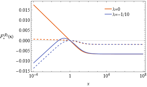
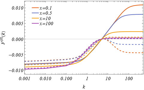
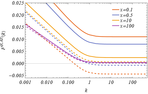
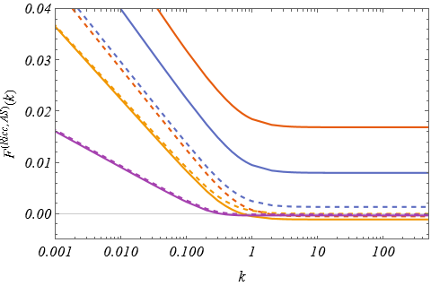
Fig. 1 shows the particular solution of the fixed-point equation for $\lambda_{k}\neq 0$ and $\lambda_{k}=0$, with $x_{0}=1$. The continuous and dashed lines correspond to $\eta_{\ast}=-2$ and $\eta_{\ast}=0$, respectively. In both cases, the fixed-point solutions vanish at $x=x_{0}$. For $\lambda_{k}=0$, the solutions become negative for $x>x_{0}$ and approach a constant asymptotic value at large $x$, in agreement with the background fixed-point form factors obtained in [83]. The inclusion of a cosmological constant mainly affects the small-$x$ regime, where a maximum develops for $x<x_{0}$. The boundary function $h$ allows one to shift the solutions, and can be used to render the large-$x$ behaviour positive if desired.

The relation between the particular solution of the fixed-point equation and the corresponding dimensional flow, $f_{k}(q^{2},\bar{\lambda})=-\int_{k}^{\Lambda}\frac{\beta_{k_{1}}\left(\eta(k_{1}),q^{2},\bar{\lambda}\right)}{k_{1}}\,dk_{1}$, can be made explicit by the change of variables $v=q^{2}/k_{1}^{2}$ (with $x_{0}=q^{2}/k_{0}^{2}$), which yields

$$\int_{x_{0}}^{x}{\frac{H\left(\eta\left(v\right),v,\frac{\lambda_{k}}{x}v\right)}{2v}dv}=-\int_{k_{0}}^{k}{\frac{H\left(\eta\left(\frac{q^{2}}{k_{1}^{2}}\right),\frac{q^{2}}{k_{1}^{2}},\frac{\bar{\lambda}}{k_{1}^{2}}\right)}{k_{1}}dk_{1}}=\int_{k}^{k_{0}}{\frac{\beta_{k}\left(q^{2},\bar{\lambda},\eta_{k_{1}}\right)}{k_{1}}dk_{1}}$$ (IV.14)

Setting $k_{0}=\Lambda$ and $\eta(k)=\eta_{*}$ shows that the fixed-point solution corresponds to the dimensional flow evaluated along a trajectory where the anomalous dimension is taken at its fixed-point value:

$$F_{\ast}^{(\mathrm{part})}\left(x=\frac{q^{2}}{k^{2}},\lambda_{k}=\frac{\bar{\lambda}}{k^{2}};x_{0}=\frac{q^{2}}{\Lambda^{2}}\right)\equiv f_{*}\left(q^{2},\bar{\lambda},\eta_{\ast};k,\Lambda\right)=-\int_{k}^{\Lambda}{\frac{\beta_{k^{\prime}}\left(q^{2},\bar{\lambda},\eta_{\ast}\right)}{k^{\prime}}dk^{\prime}}$$ (IV.15)

This establishes the equivalence between the fixed-point regime and the dimensional RG flow in the appropriate scaling limit, corresponding to the Gaussian ($m_{p}\to\infty$) or interacting (Reuter) fixed point ($m_{p}\to 0$).

The limit $x\to\infty$ and $x_{0}\to 0$ corresponds to the infrared regime $k\to 0$ with $\Lambda\to\infty$. In this limit, the two fixed-point solutions take the form

$$\begin{split}&f_{\ast,k=0}^{\left(\mathrm{R}\right)}\left(u\right)\equiv\lim_{\begin{subarray}{c}x\to+\infty\\ x_{0}\to 0\end{subarray}}{F_{\ast}^{\left(\mathrm{R}\right)}\left(u,x,x_{0}\right)}=\left(\frac{1}{1920\pi^{2}}-\frac{7\eta_{\ast}}{768\pi^{2}}\right)\ln{\left(\frac{q^{2}}{\mu^{2}}\right)}+\frac{7}{768\pi^{2}}\left(\eta_{\ast}-2\right)\ln{\left(\frac{u}{2}\right)}+\\ &+\frac{139}{28800\pi^{2}}+\frac{\left(\eta_{\ast}-2\right)\left(287u^{2}+4280u-960\right)}{23040\pi^{2}u^{2}}-\frac{\sqrt{u+8}\left(7u^{2}+72u-16\right)}{768\pi^{2}u^{\frac{5}{2}}}\left(\eta_{\ast}-2\right)\ln{\left(\frac{1+\sqrt{\frac{u}{8+u}}}{1-\sqrt{\frac{u}{8+u}}}\right)}\\ &f_{\ast,k=0}^{\left(\mathrm{\mathrm{Ricc}}\right)}\left(u\right)\equiv\lim_{\begin{subarray}{c}x\to+\infty\\ x_{0}\to 0\end{subarray}}{F_{\ast}^{\left(Ricc\right)}\left(u,x,x_{0}\right)}=\left(\frac{7}{320\pi^{2}}-\frac{7\eta_{\ast}}{384\pi^{2}}\right)\ln{\left(\frac{q^{2}}{\mu^{2}}\right)}+\frac{7}{384\pi^{2}}\left(\eta_{\ast}-2\right)\ln{\left(\frac{u}{2}\right)}-\\ &-\frac{31}{14400\pi^{2}}-\frac{\left(\eta_{\ast}-2\right)\left(103u^{2}+4640u-3840\right)}{11520\pi^{2}u^{2}}-\frac{\sqrt{u+8}\left(7u^{2}-80u+64\right)}{384\pi^{2}u^{\frac{5}{2}}}\left(\eta_{\ast}-2\right)\ln{\left(\frac{1+\sqrt{\frac{u}{8+u}}}{1-\sqrt{\frac{u}{8+u}}}\right)}\end{split}$$ (IV.16)

The fixed-point solutions at $k=0$ are non-local functions of $u$. Setting $\eta_{\ast}=0$ reproduces the EFT result in eq. (LABEL:EFTresult), so that the EFT flow can be interpreted as the fixed-point solution associated with the Gaussian fixed point of the Newton coupling. Conversely, $\eta_{\ast}=-2$ leads to a different EFT-like solution which yields the same coefficient of the logarithmic terms in both the IR and UV expansions in eqs. (III.12) and (III.20). This result will play an important role in the construction of the asymptotically safe solution.

In the massless limit $u\to\infty$ the previous expressions yield

$$\begin{split}&f_{\ast,k=0}^{\left(R\right)}\left(u\to\infty\right)=\left(\frac{1}{1920\pi^{2}}-\frac{7\eta_{\ast}}{768\pi^{2}}\right)\ln{\left(\frac{q^{2}}{\mu^{2}}\right)}+\frac{-2314+1435\eta_{\ast}}{115200\pi^{2}}+\\ &+\left(\eta_{\ast}-2\right)\left[\frac{\frac{43}{288\pi^{2}}-\frac{25\ln{\left(\frac{u}{2}\right)}}{192\pi^{2}}}{u}+\frac{-\frac{29}{64\pi^{2}}-\frac{9\ln{\left(\frac{u}{2}\right)}}{32\pi^{2}}}{u^{2}}+O\left(\frac{1}{u^{3}}\right)\right]\\ &f_{\ast,k=0}^{\left(\mathrm{Ricc}\right)}\left(u\to\infty\right)=\left(\frac{7}{320\pi^{2}}-\frac{7\eta_{\ast}}{384\pi^{2}}\right)\ln{\left(\frac{q^{2}}{\mu^{2}}\right)}+\frac{906-515\eta_{\ast}}{57600\pi^{2}}+\\ &+\left(\eta_{\ast}-2\right)\left[\frac{-\frac{137}{288\pi^{2}}+\frac{13\ln{\left(\frac{u}{2}\right)}}{96\pi^{2}}}{u}+\frac{\frac{35}{32\pi^{2}}+\frac{13\ln{\left(\frac{u}{2}\right)}}{16\pi^{2}}}{u^{2}}+O\left(\frac{1}{u^{3}}\right)\right]\end{split}$$ (IV.17)

apart from the logarithmic term, this is a power series in $\bar{\lambda}/q^{2}$ and the limit $\bar{\lambda}\rightarrow 0$ is still regular.

Figure 1: Fixed-point form factors for $\bar{\lambda}\neq 0$ (blue) and $\bar{\lambda}=0$ (beige), obtained with $m=3$ and boundary condition $F_{*}(x_{0})=0$ at $x_{0}=1$. Panels (a) and (b) show $F_{*}^{(R)}(x)$ and $F_{*}^{(\mathrm{Ricc})}(x)$, respectively. Solid and dashed lines correspond to the Reuter and Gaussian fixed points of the Newton coupling.

IV.3The perturbations around the fixed-point solution

Linearizing the flow equation around the fixed points allows one to study the critical properties of the theory. The perturbations of the Newton coupling around the non-trivial fixed point are obtained by expanding the solution for $g_{k}$ in the regime $m_{p}\ll k$, see eq. (III.9). This induces a corresponding expansion of the anomalous dimension and, consequently, of the dimensionless function $H$ in eq. (IV.3):

$$\begin{split}&H\left(\eta_{k},x,\lambda_{k}\right)=H\left(\eta_{\ast}=-2,x,\lambda_{k}\right)+\sum_{j=1}^{+\infty}{\left.\partial_{m_{p}^{2}}^{j}H\left(\eta_{k},x,\lambda_{k}\right)\right|_{m_{p}^{2}=0}\left(\frac{m_{p}}{k}\right)^{2j}}\end{split}$$ (IV.18)

Replacing this in the flow equation eq.(IV.2) shows that the solution can be written as

$$\begin{split}&F_{k}\left(x,\lambda_{k}\right)=F_{\mathrm{hom}}\left(x,\lambda_{k},k\right)+F_{\mathrm{part}}\left(x,\lambda_{k},k\right)\\ &F_{\mathrm{part}}\left(x,\lambda_{k},k\right)=F_{\ast}\left(x,\lambda_{k}\right)+\sum_{j=1}^{+\infty}{F_{j}\left(x,\lambda_{k}\right)\left(\frac{m_{p}}{k}\right)^{2j}}\end{split}$$ (IV.19)

where $F_{\mathrm{hom}}\left(x,\lambda_{k},k\right)$ is the general solution of the homogeneous equation

$$kF_{\hom}^{\left(0,0,1\right)}\left(x,\lambda_{k},k\right)=2xF_{\hom}^{\left(1,0,0\right)}\left(x,\lambda_{k},k\right)+2\lambda_{k}F_{\hom}^{\left(0,1,0\right)}\left(x,\lambda_{k},k\right)$$ (IV.20)

and $F_{j}\left(x,\lambda_{k}\right)$ are determined by

$$-2jF_{j}\left(x,\lambda_{k}\right)=2xF_{j}^{\left(1,0\right)}\left(x,\lambda_{k}\right)+2\lambda_{k}F_{j}^{\left(0,1\right)}\left(x,\lambda_{k}\right)+\left.\partial_{m_{p}^{2}}^{j}H\left(\eta_{k},x,\lambda_{k}\right)\right|_{m_{p}^{2}=0}$$ (IV.21)

Both equations are linear partial differential equations. The particular solution in Eq. (LABEL:solpert) describes a deformation of the fixed-point solution and does not affect the critical manifold. Consequently, the critical exponents are fully determined by the homogeneous solution.

The general homogeneous solution can be written as

$$F_{\mathrm{hom}}\left(x,\lambda_{k},k\right)=c\left(k\sqrt{x},\frac{\lambda_{k}}{x}\right)\,,$$ (IV.22)

where $c(a,b)$ is fixed by the boundary function. Regularity at $(x,\lambda_{k})=(0,0)$ constrains $c$ and determines the spectrum of critical exponents. The local expansion near the origin reads

$$F_{\mathrm{hom}}\left(x,\lambda_{k},k\right)=\sum_{l,m=0}^{+\infty}c_{l,m}\,k^{-\theta_{l,m}}x^{l}\lambda_{k}^{m}\,,$$ (IV.23)

with the spectrum of critical exponents determined by

$$\theta_{l,m}=-2(l+m)\,.$$ (IV.24)

This contains one marginal direction ($l+m=0$) and an infinite tower of irrelevant directions ($l+m\geq 1$). The large-$k$ asymptotics of the solutions, however, is not obtained term-by-term from $k^{-\theta_{l,m}}$, but follows from the global solution of the flow equation, which fixes the function $c\left(k\sqrt{x},\frac{\lambda_{k}}{x}\right)$. For a smooth solution in $(x,\lambda_{k})\in[0,+\infty)\times[0,+\infty)$, for $k\sqrt{x}\gg 1$, one can write

$$c\left(k\sqrt{x}\to\infty,\frac{\lambda_{k}}{x}\right)=\sum_{l,m=0}^{\infty}d_{l,m}\,k^{\theta_{l,m}}x^{-l}\lambda_{k}^{-m}\,,$$ (IV.25)

which shows that the UV scaling is controlled by the large-argument behavior of $c$. The critical exponents $\theta_{l,m}$ encode the local stability properties of the fixed point and the structure of the UV critical manifold, while the detailed ultraviolet scaling depends on the full RG flow.

The ultraviolet scaling of the particular solution is determined by eq.(LABEL:solpert), which shows that irrelevant directions are suppressed as powers of $1/k^{2}$, $1/k^{4}$, and higher, implying that the fixed point is ultraviolet attractive and infrared repulsive along these directions.

The particular solutions $F_{j}(x,\lambda_{k})$ in eq.(LABEL:solpert) are given by

$$F_{j}(x,\lambda_{k})=-x^{-j}\int_{x_{0}}^{x}\frac{\left.\partial_{m_{p}^{2}}^{j}H\!\left(\eta_{k},v,\frac{\lambda_{k}}{x}v\right)\right|_{m_{p}^{2}=0}}{2v^{1-j}}\,dv.$$ (IV.26)

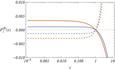
The derivatives of $H$ can be read from eq. (LABEL:expaH). The functions $F_{j}$ share the same structural form as the fixed-point solution in eq. (LABEL:solFPpart), up to the absence of leading logarithmic contributions. Fig. 3 shows $F_{j}(x,\lambda_{k})$ for $j=1$ (solid lines) and $j=2$ (dashed lines), with $x_{0}=1$. The sign of the perturbations alternates with $j$. For $\lambda_{k}=0$ (beige lines), $F_{j}$ diverges as $x^{-j}$ for $x\to 0$, while for $\lambda_{k}\neq 0$ (blue lines) it remains finite. In both cases, the large-$x$ decay is $\sim 1/x$.

In the limits $\left(x_{0},x\right)\rightarrow(0,+\infty)$, the solution eq.(LABEL:solpert) is given by

$$f_{k=0}^{(i)}\left(u,w\right)=f_{\ast,k=0}^{\left(i\right)}\left(u\right)+\sum_{n=1}^{+\infty}\frac{L_{n}\left(u\right)}{w^{n}}$$ (IV.27)

where $i=\mathrm{R}$, $\mathrm{Ricc}$. The series coefficients $L_{n}\left(u\right)$ are non-local functions of $u$ as in the fixed-point case. The first terms of the series are given by

$$\begin{split}&L_{1}^{\left(R\right)}\left(u\right)\frac{\left(25u^{2}+208u-80\right)\ln{\left(\frac{1+\sqrt{\frac{u}{u+8}}}{1-\sqrt{\frac{u}{u+8}}}\right)}}{736\pi\sqrt{u^{3}\left(u+8\right)}}+\frac{\frac{60}{u}-161}{2208\pi}\\ &L_{2}^{\left(R\right)}=\frac{9\left(9u^{2}+56u-80\right)\ln{\left(\frac{1+\sqrt{\frac{u}{u+8}}}{1-\sqrt{\frac{u}{u+8}}}\right)}}{2116\sqrt{u}\left(u+8\right)^{\frac{3}{2}}}-\frac{3\left(25u^{2}+188u-240\right)}{8464\left(u+8\right)}\end{split}$$ (IV.28)

and

$$\begin{split}&L_{1}^{\left(\mathrm{Ricc}\right)}\left(u\right)=\frac{\left(-13u^{2}-208u+320\right)\ln{\left(\frac{1+\sqrt{\frac{u}{u+8}}}{1-\sqrt{\frac{u}{u+8}}}\right)}}{368\pi\sqrt{u^{3}\left(u+8\right)}}+\frac{11-\frac{15}{u}}{69\pi}\\ &L_{2}^{\left(\mathrm{Ricc}\right)}=\frac{3\left(13u^{2}+128u-960\right)}{4232\left(u+8\right)}-\frac{9\left(13u^{2}+16u-320\right)\ln{\left(\frac{1+\sqrt{\frac{u}{u+8}}}{1-\sqrt{\frac{u}{u+8}}}\right)}}{1058\sqrt{u}\left(u+8\right)^{\frac{3}{2}}}\end{split}$$ (IV.29)

Higher-order coefficients follow the same pattern. The decoupling and massless limits reproduce the same behavior of the previous cases. In the strict $u\to\infty$ limit, all $L_{n}^{(i)}$ approach constants.

A similar analysis applies to the Gaussian fixed point $g_{\ast}=0$, obtained by expanding the Newton coupling in the limit $m_{p}\gg k$ ($m_{p}\to\infty$). The beta function then admits the expansion

$$\begin{split}&H\left(\eta_{k},x,\lambda_{k}\right)=H\left(\eta_{\ast}=0,x,\lambda_{k}\right)+\sum_{j=1}^{+\infty}{\left.\partial_{k^{2}}^{j}H\left(\eta_{k},x,\lambda_{k}\right)\right|_{k^{2}=0}\left(\frac{k}{m_{p}}\right)^{2j}}\end{split}$$ (IV.30)

The corresponding particular solution reads

$$F_{\mathrm{part}}^{(\eta_{*}=0)}\left(x,\lambda_{k},k\right)=F_{\ast}^{(\eta_{*}=0)}\left(x,\lambda_{k}\right)+\sum_{j=1}^{+\infty}{F_{j}^{(\eta_{*}=0)}\left(x,\lambda_{k}\right)\left(\frac{k}{m_{p}}\right)^{2j}}$$ (IV.31)

where $F_{j}^{(\eta_{*}=0)}\left(x,\lambda_{k}\right)$ satisfy

$$2jF_{j}\left(x,\lambda_{k}\right)=2xF_{j}^{\left(1,0\right)}\left(x,\lambda_{k}\right)+2\lambda_{k}F_{j}^{\left(0,1\right)}\left(x,\lambda_{k}\right)+\left.\partial_{k^{2}}^{j}H\left(\eta_{k},x,\lambda_{k}\right)\right|_{k^{2}=0}$$ (IV.32)

The perturbations are governed by the critical exponents $\theta=-2j$, $j=1,2,\ldots$, implying that the Gaussian fixed point is IR attractive and UV repulsive in the space of form-factor perturbations.

The solutions of eq. (IV.32) are given by

$$F_{j}(x,\lambda_{k};x_{0})=-x^{j}\int_{x_{0}}^{x}\frac{\left.\partial_{k^{2}}^{j}H\!\left(\eta_{k},v,\frac{\lambda_{k}}{x}v\right)\right|_{k^{2}=0}}{2v^{1+j}}\,dv.$$ (IV.33)

The functions $F_{j}$ exhibit the same functional form as the fixed-point solution in eq. (LABEL:solFPpart), with $\eta_{*}=0$. Fig. 3 shows $F_{j}(x,\lambda_{k})$ for $j=1$ (solid lines) and $j=2$ (dashed lines), with $x_{0}=1$. As in the case of perturbations around the UV form factor fixed-point, the sign of the solutions alternates with increasing $j$. For $x>x_{0}$, the scaling behavior is governed by $x^{j}$, whereas for $x<x_{0}$ the solutions approach a constant value. This behavior holds both for $\lambda_{k}=0$ and $\lambda_{k}\neq 0$.

In the limits $(x_{0},x)\to(0,\infty)$, eq.(IV.33) reproduce the IR behaviour of Eq. (III.12), provided standard renormalization conditions at $k=\Lambda$ are imposed. Further details on the relation between flow equations, fixed points, and renormalization are given in Appendix B.

Figure 2: Plots of the perturbations $F_{j}(x,\lambda_{k})$ with $j=1$ (continued lines) and $j=2$ (dashed lines) around the UV fixed-point $F_{*}^{(\eta_{*}=2)}(x,\lambda_{k})$. Panels (a) and (b) shows $F_{j}^{(\mathrm{R})}(x,\lambda_{k})$ and $F_{j}^{(\mathrm{Ricc})}(x,\lambda_{k})$ respectively. Beige and blue lines correspond to the $\lambda_{k}=0$ and $\lambda_{k}\neq 0$ respectively.

Figure 3: Plots of the perturbations $F_{j}(x,\lambda_{k})$ with $j=1$ (continued lines) and $j=2$ (dashed lines) around the IR fixed-point $F_{*}^{(\eta_{*}=0)}(x,\lambda_{k})$. Panels (a) and (b) shows $F_{j}^{(\mathrm{R})}(x,\lambda_{k})$ and $F_{j}^{(\mathrm{Ricc})}(x,\lambda_{k})$ respectively. Beige and blue lines correspond to the $\lambda_{k}=0$ and $\lambda_{k}\neq 0$ respectively.

Eq. (LABEL:solpert) shows that the flow of the form factor approaches the non-Gaussian fixed point in the ultraviolet:

$$\lim_{k\to\infty}F_{k}(x,\lambda_{k})=F_{\ast}^{(\eta_{*}=-2)}(x,\lambda_{k})\,,$$ (IV.34)

ensuring a well-defined continuum limit at the level of dimensionless variables. However, reverting to dimensional variables, $F_{k}(x)\to f_{k}(q^{2})$ via Eq. (IV.14), a logarithmic divergence reappears in the limit $k\to\infty$ of the dimensionful form factor (Eq. (LABEL:FPk0)). This indicates that asymptotic safety of the dimensionless flow does not automatically guarantee regular ultraviolet behavior of the dimensional form factor. The mismatch originates from the additional physical scale $q^{2}$, which prevents a direct identification of the limits $\lim_{k\to\infty}F_{k}(x)$ and $\lim_{k\to\infty}f_{k}(q^{2})$. In the following, we discuss the properties of the integrated flow and show how to construct a dimensionful asymptotically safe form factor free of ultraviolet divergences.

IV.4The properties of the adimensional flow

The general solution of eq.(IV.2) reads

$$F_{k}\left(a^{2},\lambda_{k}\right)=c\left(k\sqrt{x},\frac{\lambda_{k}}{x}\right)-\int_{x_{\mathrm{B}}}^{x}{\frac{H\left(\eta\left(k\sqrt{\frac{x}{v}}\right),v,\frac{\lambda_{k}}{x}v\right)}{2v}dv}$$ (IV.35)

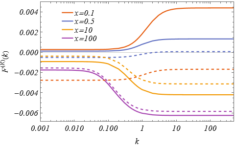
where $c\left(k\sqrt{x},\frac{\lambda_{k}}{x}\right)$ is fixed by eq.(IV.22) and $x_{\mathrm{B}}$ is an arbitrary normalization scale. The integral defines the bulk solution. Fig. 6 displays, for different values of $x$ and $\lambda_{k}$, the bulk asymptotically safe flow connecting the two fixed points $F_{*}^{(\eta_{*}=0)}(x,\lambda_{k})$ and $F_{*}^{(\eta_{*}=-2)}(x,\lambda_{k})$. Deviations from the EFT behaviour set in at $k\sim m_{p}$, above which the flow enters the asymptotically safe regime.

The choice of boundary condition fixes $c$ and selects a specific RG trajectory within the space of solutions. Imposing that at the scale $k=\Lambda$ the solution satisfies $F_{\Lambda}(x,\lambda_{\Lambda})=U_{\Lambda}(x,\lambda_{\Lambda})$, with $U_{\Lambda}$ an arbitrary function, the resulting trajectory takes the form:

$$\begin{split}&F_{k}\left(x,\lambda_{k};\Lambda\right)=U_{\Lambda}\left(\frac{k^{2}x}{\Lambda^{2}},\frac{k^{2}\lambda_{k}}{\Lambda^{2}}\right)-\left[\int_{x_{\mathrm{B}}}^{x}{\frac{H\left(\eta\left(k\sqrt{\frac{x}{v}}\right),v,\frac{\lambda_{k}}{x}v\right)}{2v}dv}+\int_{\frac{k^{2}x}{\Lambda^{2}}}^{x_{\mathrm{B}}}{\frac{H\left(\eta\left(k\sqrt{\frac{x}{v}}\right),v,\frac{\lambda_{k}}{x}v\right)}{2v}dv}\right]=\\ &=U_{\Lambda}\left(\frac{k^{2}x}{\Lambda^{2}},\frac{k^{2}\lambda_{k}}{\Lambda^{2}}\right)-\int_{\frac{k^{2}x}{\Lambda^{2}}}^{x}\frac{H\left(\eta\left(\frac{k\sqrt{x}}{\sqrt{v}}\right),v,\frac{\lambda_{k}}{x}v\right)}{2v}\,dv\,.\end{split}$$ (IV.36)

The combination $k^{2}x/\Lambda^{2}$ follows from the characteristic structure of the PDE. The boundary choice enters as an additional contribution to the bulk term. This does not represent an independent dynamical sector of the RG flow, but rather encodes how the UV data at $k=\Lambda$ are propagated along the flow to lower scales. From eq.(IV.14) the total integral coincides the dimensional flow expressed in dimensionless variables. Indeed, one can rewrite it as

$$\int_{\frac{k^{2}x}{\Lambda^{2}}}^{x}\frac{H\left(\eta\left(\frac{k\sqrt{x}}{\sqrt{v}}\right),v,\frac{\lambda_{k}}{x}v\right)}{2v}\,dv=\int_{k}^{\Lambda}\frac{\beta_{k_{1}}\left(\eta_{k_{1}},q^{2},\bar{\lambda}\right)}{k_{1}}\,dk_{1}\,,$$ (IV.37)

which makes explicit the equivalence with the integrated form of the flow derived in Sec. III.

Figure 6 illustrates, for $U_{\Lambda}=0$, the impact of the boundary contribution on the bulk flow. For $k\ll m_{p}$, the solution continues to evolve and no stationary regime is reached in the IR limit $k\to 0$, whereas for $k\gg m_{p}$ the flow approaches the UV fixed-point regime. In the Gaussian regime, the solution is equivalent to Eq. (IV.31) with $x_{0}\equiv k^{2}x/\Lambda^{2}$:

$$\begin{split}&F_{k}\left(x,\lambda_{k},\frac{k}{m_{p}}\ll 1;\Lambda\right)=F_{\ast}^{\left(\eta_{\ast}=0\right)}\left(x,\lambda_{k};\frac{k^{2}x}{\Lambda^{2}}\right)+\sum_{j=1}^{+\infty}{F_{j}^{\left(\eta_{\ast}=0\right)}\left(x,\lambda_{k};\frac{k^{2}x}{\Lambda^{2}}\right)\left(\frac{k^{2}}{m_{p}^{2}}\right)^{j}}=\\ &=\sum_{j=0}^{+\infty}{\left[F_{j}^{\left(\eta_{\ast}=0\right)}\left(x,\lambda_{k};x_{\mathrm{B}}\right)+F_{j}^{\left(\eta_{\ast}=0\right)}\left(x_{\mathrm{B}},\lambda_{k};\frac{k^{2}x}{\Lambda^{2}}\right)\right]\left(\frac{k^{2}}{m_{p}^{2}}\right)^{j}}\end{split}$$ (IV.38)

In the limit $k\to 0$, the boundary term $F_{j=0}^{(\eta_{\ast}=0)}\!\left(x_{\mathrm{B}},\lambda_{k};k^{2}x/\Lambda^{2}\right)$ generates a residual logarithmic piece $a_{\mathrm{EFT}}\ln(k^{2}x/\Lambda^{2})$, with $a_{\mathrm{EFT}}$ given in Eq. (LABEL:EFTIR). The small-$k$ behaviour then reads

$$F_{k}\left(x,\lambda_{k};\Lambda\right)=F_{\ast}^{\left(\eta_{\ast}=0\right)}\left(x,\lambda_{k}\right)+a_{\mathrm{EFT}}\ln\left(\frac{k^{2}x}{\Lambda^{2}}\right)+O\left(k^{2}\right)$$ (IV.39)

indicating that, although the flow is controlled by the Gaussian fixed point, the integrated RG trajectory does not become stationary in the infrared limit. This is not in contradiction with the previous analysis of the IR attractiveness of the fixed point. The residual logarithmic term does not arise from a perturbative expansion around the fixed point, but instead from the propagation of the UV data at $k=\Lambda$ to infrared scales. Moreover, it does not originate from the expansion of Eq. (LABEL:ASflow) around $x=0$, which remains analytic as reflected in the structure of Eq. (IV.22).

The residual logarithmic dependence is necessary to reproduce the correct infrared behaviour of the dimensionful form factor. Indeed, in the limits $x\to\infty$ and $k\to 0$, Eq. (LABEL:flowIRintegr) reproduces the full IR expansion of Eq. (III.12) after identifying $k^{2}x=q^{2}$ and removing the cutoff $\Lambda$ via a renormalization condition. Similarly, expanding Eq. (LABEL:ASflow) in the regime $m_{p}^{2}\ll k^{2}$ and taking $(x,\Lambda)\to\infty$ using $k^{2}x=q^{2}$ reproduces the UV expansion of Eq. (III.20). This establishes a direct relation between the asymptotic regimes of the integrated dimensionless flow and the corresponding IR and UV expansions at $k=0$ of the dimensional flow.

Figure 4: Bulk flow of the asymptotically safe solution in Eq. (IV.35) for different values of $x$. Panels (a) and (b) show $F_{k}^{(\mathrm{R})}(x,\lambda_{k})$ and $F_{k}^{(\mathrm{Ricc})}(x,\lambda_{k})$, respectively. The full and dashed line correspond to $\lambda_{k}=0$ and $\lambda_{k}\neq 0$ respectively. The plots are obtained fixing $m_{p}=1$, $x_{\mathrm{B}}=1$.

Figure 5: Flow of the integrated asymptotically safe solution in Eq. (LABEL:ASflow) for different values of $x$. Panels (a) and (b) show $F_{k}^{(\mathrm{R})}(x,\lambda_{k})$ and $F_{k}^{(\mathrm{Ricc})}(x,\lambda_{k})$, respectively. The full and dashed line correspond to $\lambda_{k}=0$ and $\lambda_{k}\neq 0$ respectively. The plots are obtained fixing $m_{p}=1$, $\Lambda=5m_{p}$, and $U_{\Lambda}=0$.

Figure 6: Flow of the asymptotically safe renormalized solution in Eq. (LABEL:ASsoladim) for different values of $x$. Panels (a) and (b) show $F_{k}^{(\mathrm{R})}(x)$ and $F_{k}^{(\mathrm{Ricc})}(x)$, respectively. The full and dashed line correspond to $\lambda_{k}=0$ and $\lambda_{k}\neq 0$ respectively. The plots are obtained fixing $m_{p}=1$ and $h=0$.

IV.5The asymptotically safe renormalized solution

Although the flow is controlled by the non-Gaussian fixed point in the UV, the integrated form factor still exhibits the logarithmic behavior in the limit $\Lambda\to\infty$. As already anticipated, asymptotic safety of the dimensionless flow is not sufficient to guarantee a finite integrated form factor. An additional renormalization condition is required. The result of Sec. III is recovered by choosing

$$U_{\Lambda}(x,\lambda_{\Lambda})=\alpha\ln\left(\frac{\mu^{2}}{\Lambda^{2}}\right)\,,$$ (IV.40)

where $\alpha$ is the universal coefficient in Eq. (III.12). In RG terms, this choice selects the perturbatively renormalizable trajectory, yielding a well-defined $\Lambda\to\infty$ limit in the EFT sense.

Within the asymptotic safety framework, however, physical consistency requires the absence of external renormalization scales in the ultraviolet scaling behavior. The perturbatively renormalizable trajectory is therefore not compatible with a consistent asymptotically safe flow. Consistency between ultraviolet fixed-point scaling and finiteness of the dimensional form factor instead selects the non-trivial fixed-point solution as boundary condition:

$$U_{\Lambda}(x,\lambda_{\Lambda})=F_{*}^{(\eta_{*}=-2)}(x,\lambda_{\Lambda};x_{0})\,.$$ (IV.41)

We refer to this choice as an asymptotically safe renormalization condition. With this prescription, the solution takes the form

$$\begin{split}&F_{k}\left(x,\lambda_{k};\Lambda,x_{0}\right)=\\ &=h\left(x_{0},\frac{x_{0}\lambda_{k}}{x}\right)+F_{\ast}^{(\eta_{*}=-2)}\left(x,\lambda_{k};x_{0}\right)-\int_{\frac{k^{2}x}{\Lambda^{2}}}^{x}\left[\frac{H\left(\eta\left(k\sqrt{\frac{x}{v}}\right),v,\frac{\lambda_{k}}{x}v\right)}{2v}-\frac{H\left(\eta_{\ast}=-2,v,\frac{\lambda_{k}}{x}v\right)}{2v}\right]dv\end{split}$$ (IV.42)

The key feature is the difference between the full and fixed-point beta-function contributions. This subtraction cancels the logarithmic terms in the limit $\Lambda\to\infty$ without introducing an external scale $\mu$, leading to a qualitatively different infrared behavior from the perturbative case. In contrast, if the Gaussian fixed point with $\eta_{*}=0$ is chosen, the subtraction reproduces the standard logarithmic behavior $\sim\ln(q^{2}/\mu^{2})$.

The solution (LABEL:ASsoladim) still preserves the asymptotically safe UV behavior. Indeed, as $k\to\infty$ one has $\eta\!\left(\frac{k\sqrt{x}}{\sqrt{v}}\right)\to\eta_{\ast}$, so that the integrand vanishes and Eq. (LABEL:ASsoladim) reduces to the non-Gaussian fixed-point solution, independently of the choice of the UV scale $\Lambda$ (see Fig. 6).

This prescription differs from the standard perturbative one, where divergences are absorbed into couplings via counterterms and the resulting trajectories remain close to the Gaussian fixed point, displaying logarithmic running $\sim\ln(\mu^{2}/k^{2})$. Instead, imposing eq. (IV.41) selects a trajectory on the critical surface of the non-Gaussian fixed point. The RG flow then remains finite as $\Lambda\to\infty$, with the logarithmic dependence dynamically suppressed rather than subtracted. Consequently, the dependence on the renormalization scale $\mu$ is absent in the asymptotically safe solution. The remaining parameter $x_{0}=q^{2}/k_{0}^{2}$ arises as an integration constant of the fixed-point equation and does not originate from the subtraction of ultraviolet divergences. Predictivity is controlled by the relevant directions of the fixed point. In the present one-loop approximation, no such directions arise, so that no additional free parameters appear.

This construction becomes particularly relevant when expressed in terms of dimensional variables, where the solution takes the form

$$\begin{split}&F_{k}\left(\frac{q^{2}}{k^{2}},\frac{\bar{\lambda}}{k^{2}};\Lambda,\frac{q^{2}}{k_{0}^{2}}\right)=h\left(\frac{q^{2}}{k_{0}^{2}},\frac{\bar{\lambda}}{k_{0}^{2}}\right)+\int_{k_{0}}^{\Lambda}{\frac{\beta_{k^{\prime}}\left(q^{2},\bar{\lambda},\eta_{\ast}=-2\right)}{k^{\prime}}dk^{\prime}}-\int_{k}^{\Lambda}{\frac{\beta_{k^{\prime}}\left(q^{2},\bar{\lambda},\eta_{k^{\prime}}\right)}{k^{\prime}}dk^{\prime}}\end{split}$$ (IV.43)

Eq. (LABEL:ASsol) shows that the asymptotically safe dimensional form factor is obtained by subtracting the fixed-point contribution from the full RG evolution, up to the boundary term encoded in $h$. The reference scale $k_{\mathrm{0}}$ can be chosen arbitrarily, including $k_{\mathrm{0}}=0$, reflecting its role as an integration constant rather than a renormalization scale.

Eq. (LABEL:ASsol) admits two complementary interpretations when related to the dimensional flow equation. The first arises by implementing the non-perturbative renormalization condition directly at the level of the dimensional flow,

$$k\partial_{k}f_{k}(q^{2},\bar{\lambda})=\beta_{k}(q^{2},\bar{\lambda}),\qquad f_{k=\Lambda}(q^{2},\bar{\lambda})=f_{*}\left(q^{2},\bar{\lambda},\eta_{\ast};k_{0},\Lambda\right)+h\left(\frac{q^{2}}{k_{0}^{2}},\frac{\bar{\lambda}}{k_{0}^{2}}\right),$$ (IV.44)

The AS form factor is obtained from the dimensional flow by fixing the boundary condition to the UV fixed-point solution $f_{*}\left(q^{2},\bar{\lambda},\eta_{\ast};k_{0},\Lambda\right)$, defined in Eq. (IV.15). This ensures consistency between the dimensionless and dimensionful formulations, $\lim_{k\to\infty}F_{k}(x)=\lim_{k\to\infty}f_{k}(q^{2})$.

The second interpretation follows directly from Eq. (LABEL:ASsol) and can be formulated entirely at the level of the beta functions:

$$k\partial_{k}f_{k}(q^{2},\bar{\lambda})=\beta_{k}(q^{2},\bar{\lambda};\eta_{k}\neq 0)-\beta_{k}(q^{2},\bar{\lambda};\eta_{*}=-2)(1-\theta(k-k_{0})),\qquad f_{k=\Lambda}(q^{2},\bar{\lambda})=h\left(\frac{q^{2}}{k_{0}^{2}},\frac{\bar{\lambda}}{k_{0}^{2}}\right)$$ (IV.45)

where $\theta(t)$ is the Heaviside function. In this form, the flow is driven by the difference between the full beta function and its fixed-point counterpart, while the boundary condition at $k=\Lambda$ is encoded in $h$. This representation is particularly convenient for numerical implementations, as it avoids the explicit computation of the fixed-point solution.

The asymptotically safe solution in Eq. (LABEL:ASsol) is defined up to an arbitrary function $h\!\left(x_{0},x_{0}\frac{\lambda_{k}}{x}\right)$, encoding the choice of boundary conditions for the fixed-point equation. This freedom allows one to select different asymptotic behaviours in the infrared and ultraviolet regimes. For $\bar{\lambda}=0$, $h$ reduces to a constant, $h(x_{0})\equiv c$. The minimal choice $h=0$ defines a reference solution in which the form factors vanish in the ultraviolet, $\lim_{q^{2}\to\infty}f_{k}(q^{2})=0$, thereby isolating the intrinsic RG running.

At $k=0$ with $k_{0}=0$, the AS renormalized form factors in the IR and UV regime are obtained using eq.(LABEL:ASsol). In the IR regime the general structure of the solution is given by

$$f_{k=0}^{(i,\mathrm{AS})}\left(u,t,w\rightarrow 0\right)=\tilde{A}_{0}^{(i)}(u,w)+\sum_{n=1}^{+\infty}{A_{n}^{(i)}\left(u\right)w^{n}}$$ (IV.46)

where $i=\mathrm{R},\mathrm{Ricc}$, $\tilde{A}_{0}^{(i)}(u,w)$ is given for the two form factors respectively by

$$\begin{split}&\tilde{A}_{0}^{\left(\mathrm{R}\right)}\left(u,w\right)=\frac{287u^{2}+4280u-960}{11520\pi^{2}u^{2}}-\frac{7\ln{\left(\frac{23}{6\pi}\frac{w}{u}\right)}}{384\pi^{2}}-\frac{\sqrt{u+8}\left(7u^{2}+72u-16\right)\ln{\left(\frac{1+\sqrt{\frac{u}{u+8}}}{1-\sqrt{\frac{u}{u+8}}}\right)}}{384\pi^{2}u^{\frac{5}{2}}}\\ &\tilde{A}_{0}^{\left(\mathrm{Ricc}\right)}\left(u,w\right)=\frac{-103u^{2}-4640u+3840}{5760\pi^{2}u^{2}}-\frac{7\ln{\left(\frac{23}{6\pi}\frac{w}{u}\right)}}{192\pi^{2}}-\frac{\sqrt{u+8}\left(7u^{2}-80u+64\right)\ln{\left(\frac{1+\sqrt{\frac{u}{u+8}}}{1-\sqrt{\frac{u}{u+8}}}\right)}}{192\pi^{2}u^{\frac{5}{2}}}\end{split}$$ (IV.47)

and $A_{n}$ with $n>1$ are the IR-series coefficients defined in Eq. (III.12). In this regime, the logarithmic contribution persists but depends only on the combination $w/u=t=\bar{\lambda}/m_{p}^{2}$, effectively replacing the unphysical scale $\Lambda$ with $m_{p}$. The massless limit ($u\to\infty$) of $\tilde{A}_{0}^{(i)}$ admits a regular expansion in $1/u$, implying a smooth $\bar{\lambda}\to 0$ limit. However, the limit $w\to 0$ is singular due to the residual logarithmic term $\ln(w)$. Conversely, in the decoupling regime $u\to 0$ ($\bar{\lambda}\to\infty$), the singularity at $w=0$ disappears, but the limit $\bar{\lambda}\to 0$ becomes non-smooth.

In the UV regime we get

$$\begin{split}&f_{k=0}^{\left(\mathrm{R,AS}\right)}\left(u\rightarrow\infty,t\rightarrow 0,w\rightarrow\infty\right)=\frac{86-75\ln{\left(\frac{u}{2}\right)}}{288\pi^{2}u}-\frac{29+18\ln{\left(\frac{u}{2}\right)}}{32\pi^{2}u^{2}}+O\left(\frac{1}{u^{3}}\right)\\ &+\frac{\frac{-86+75\ln{\left(\frac{23w}{12\pi}\right)}}{2208\pi}+\frac{t\left(-97+150\ln{\left(\frac{23w}{12\pi}\right)}\right)}{576\pi^{2}}+O\left(t^{2}\right)}{w}+O\left(\frac{1}{w^{2}}\right)\\ &f_{k=0}^{\left(\mathrm{Ricc,AS}\right)}\left(u\rightarrow\infty,t\rightarrow 0,w\rightarrow\infty\right)=\frac{-137+39\ln{\left(\frac{u}{2}\right)}}{144\pi^{2}u}+\frac{35+26\ln{\left(\frac{u}{2}\right)}}{16\pi^{2}u^{2}}+O\left(\frac{1}{u^{3}}\right)\\ &+\frac{\frac{137-39\ln{\left(\frac{23w}{12\pi}\right)}}{1104\pi}+\frac{t\left(235-78\ln{\left(\frac{23w}{12\pi}\right)}\right)}{288\pi^{2}}+O\left(t^{2}\right)}{w}+O\left(\frac{1}{w^{2}}\right)\end{split}$$ (IV.48)

the asymptotically safe solution contains no isolated logarithmic contribution and admits an expansion in inverse powers of $q^{2}$. The general structure can be written as

$$f_{k=0}\left(u\to\infty,t\to 0,w\rightarrow\infty\right)=\sum_{n=1}^{+\infty}\frac{\tilde{a}_{n}+\tilde{b}_{n}\ln\left(\frac{u}{2}\right)}{u^{n}}+\sum_{n=1}^{+\infty}\frac{\sum_{m=0}^{+\infty}\left(c_{nm}+d_{nm}\ln\left(\frac{23w}{12\pi}\right)\right)t^{m}}{w^{n}}$$ (IV.49)

where $\tilde{a}_{n}$ and $\tilde{b}_{n}$ are determined by the difference between the EFT and fixed-point coefficients in the large-$u$ expansion.

V  The numerical analysis

In this section, we present the numerical analysis for the flow of form factors to arrive at $k=0$ for generic momenta. We first consider the case of the mixed scheme. This provides both a consistency check of the analytical results derived in the previous sections and a benchmark for understanding the numerical behaviour of the full $\epsilon=1$ (scheme B) case.

V.1The numerical analysis of the mixed scheme case

To perform the numerical integration, we fix $m_{p}=1$, $\bar{\lambda}=-1/10$, $\Lambda=150m_{p}$, and $m=3$. For each value of $q^{2}$ below the numerical cutoff, the flow is integrated from $k=\Lambda$ down to $k=10^{-8}$ with boundary condition $f_{k=\Lambda}(q^{2})=0$, defining the reference form factors.

Fig. 9 compares the numerical solutions with the asymptotic expansions in eqs. (III.12) and (III.20) (blue and black dashed lines, respectively). The IR expansion reproduces the flow only for $q^{2}\ll 1$, whereas the UV expansion agrees well for $q^{2}\gtrsim 5$. Both form factors develop a minimum, located at approximately $q^{2}\sim 4.5$ and $q^{2}\sim 0.25$ for the Ricci-scalar and Ricci-tensor sectors, respectively.

For comparison with the B scheme, we also solve the flow for $\bar{\lambda}=0$ (blue curves in Fig. 9). In this case the minima disappear and the logarithmic growth sets in already at small momenta. At large $q^{2}$, where the logarithmic term dominates, the $\bar{\lambda}\neq 0$ and $\bar{\lambda}=0$ solutions progressively approach each other.

Since the coefficient of the logarithmic term is positive, the form factors eventually cross zero and become positive at sufficiently large $q^{2}$. The zero can be estimated from the UV asymptotic expansion by solving $f_{k=0}(q^{2})=0$ in Eq. (III.20), yielding for $\Lambda=150m_{p}$

$$q_{R}^{2}\approx 7.4\cdot 10^{6}m_{p}^{2},\quad\quad q^{2}_{Ricc}\approx 3.8\cdot 10^{5}m_{p}^{2}.$$ (V.1)

These values lie deep in the UV region ($q^{2}\gg m_{p}^{2}$), as shown in Fig. 12. However, they should not be interpreted as physical scales, since their position depends on the UV boundary condition and can be shifted arbitrarily.

Figure 7: Numerical form factors at $k=0$ and comparison with the asymptotic analytical results. Panels (a) and (b) show $f_{k=0}^{(R)}(q^{2})$ and $f_{k=0}^{(\mathrm{Ricci})}(q^{2})$, respectively. The form factors develop a minimum in the crossover region between the IR and UV regimes. At large $q^{2}$, the logarithmic behavior dominates and the dependence on $\bar{\lambda}$ becomes negligible.

Figure 8: Reference asymptotically safe form factors at $k=0$ and comparison with the asymptotic analytical results. Panels (a) and (b) show $f_{k=0}^{(\mathrm{R})}(q^{2})$ and $f_{k=0}^{(\mathrm{Ricc})}(q^{2})$, respectively. Both form factors decay as $1/q^{2}$ at large $q^{2}$. The inset in (b) zooms into the IR region of $f_{k=0}^{(Ricc)}(q^{2})$.

Figure 9: Absolute difference $\delta f(q^{2},m_{1}=3,m_{2})$ at $k=0$ for different values of $m_{2}$. The residual regulator dependence is suppressed at large $q^{2}$.

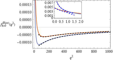
To obtain the numerical asymptotically safe (AS) form factors, we use Eq. (IV.45). The red and blue curves in Fig. 9 correspond to $\bar{\lambda}\neq 0$ and $\bar{\lambda}=0$, respectively, while the dashed lines show the analytical asymptotics in Eqs. (IV.46) and (LABEL:ASUV), derived from Eq. (LABEL:ASsol) and providing a non-trivial consistency check. The AS form factor $f_{k=0}^{(\mathrm{R,AS})}(q^{2})$ remains positive for all $q^{2}$, while $f_{k=0}^{(\mathrm{Ricc,AS})}(q^{2})$ crosses zero and approaches the UV limit $f_{k=0}^{(\mathrm{Ricc,AS})}(q^{2}\to\infty)\to 0$ from below. As discussed in Subsec. IV.5, this behaviour depends on the boundary conditions and can be shifted, e.g. by choosing $c_{\mathrm{Ricci}}$ such that $f_{\mathrm{AS}}^{(\mathrm{Ricc})}(q^{2})>0$. The $\bar{\lambda}=0$ case shows the same qualitative behaviour, unlike the non-AS solution.

In the EFT result of Eq. (LABEL:EFTresult), the dependence on the cutoff parameter $m$ at $k=0$ reduces to a constant term $c(m)$, which can be removed by an appropriate choice of boundary conditions. In the full computation, this can be tested numerically by comparing solutions at different $m$ through

$$\delta f(q^{2},m_{1},m_{2})=\left|f_{k=0}(q^{2},m_{1})-f_{k=0}(q^{2},m_{2})\right|.$$ (V.2)

Choosing $m_{1}=3$ as a reference, Fig. 9 shows $\delta f(q^{2},3,m_{2})$ for various $m_{2}$. Differently from the EFT case, the $m$-dependence propagates through the full RG flow and does not reduce to a simple additive contribution. The resulting variation therefore provides a quantitative measure of the residual regulator dependence associated with the truncation. $\delta f(q^{2},m_{1},m_{2})$ approaches a constant at large $q^{2}$, reflecting the fact that the non-universal corrections become subleading and the form factor approaches the universal logarithmic regime $\sim c(m)+\alpha\ln(q^{2}/\Lambda^{2})$.

V.2The numerical analysis in the B scheme case

In the $\epsilon=1$ scheme, the running Newton coupling is obtained numerically by solving the flow equation at $\bar{\lambda}=0$ with boundary condition $g(k_{0})=k_{0}^{2}/m_{p}^{2}$, choosing $k_{0}=10^{-8}$ and $m_{p}=1$. The flow is integrated up to $k=5000\,m_{p}$ for different cutoff values $m=3,6,8,10$, and the form-factor flow is computed as in the previous subsection. The deep ultraviolet regime is then extracted by fitting the numerical solution to the asymptotic expansion (III.20).

Fig. 12 shows the results for $m=3$, together with a comparison with the mixed-scheme (MS) case. The qualitative behavior is essentially identical in the two schemes across all momentum regimes. The difference $\delta f(q^{2})=|f_{\mathrm{B}}(q^{2})-f_{\mathrm{MS}}(q^{2})|$ (insets of Fig. 12) remains below $\mathcal{O}(10^{-2})$ and decreases with increasing $q^{2}$, indicating a weak dependence on the choice of $\epsilon$. In particular, the ultraviolet logarithmic terms exhibit universal coefficients, consistent with Eq. (III.12).

The cutoff dependence is illustrated in Fig. 12 through the difference $\delta f(q^{2},3,m_{2})$. As in the mixed scheme case, the $m$-dependence propagates through the full RG flow and does not reduce to a simple additive contribution. No qualitative differences with respect to the mixed scheme are observed.

Figure 10: Numerical form factors at $k=0$ with $\bar{\lambda}=0$ in the B scheme, compared with the mixed-scheme results of Fig. 9. Panels (a) and (b) show $f_{k=0}^{(\mathrm{R})}(q^{2})$ and $f_{k=0}^{(\mathrm{Ricc})}(q^{2})$, respectively, on a log–log scale. The insets display $\delta f(q^{2})=|f_{\mathrm{B}}(q^{2})-f_{\mathrm{MS}}(q^{2})|$. The two schemes yield nearly identical form factors, confirming the universality of the logarithmic behavior.

Figure 11: Asymptotically safe form factors at $k=0$ with $\bar{\lambda}=0$ in the B scheme, compared with the mixed-scheme results of Fig. 9. Panels (a) and (b) show $f_{k=0,\mathrm{AS}}^{(\mathrm{R})}(q^{2})$ and $f_{k=0,\mathrm{AS}}^{(\mathrm{Ricc})}(q^{2})$, respectively, on a log–log scale. The functional structure of the AS form factors is independent of $\epsilon$.

Figure 12: Absolute difference $\delta f(q^{2},m_{1}=3,m_{2})$ in the B scheme at $k=0$ for different values of $m_{2}$. The qualitative behavior is the same as in the mixed-scheme case of Fig. 9.

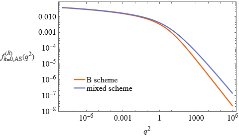
The asymptotically safe solutions are shown in Fig. 12, displaying the same qualitative features observed in Fig. 9. In particular, the log-log plot highlights the asymptotic behavior $f(q^{2}\to\infty)\sim\frac{a+b\ln(q^{2})}{q^{2}}$. The absence of a pure logarithmic term provides an additional consistency check of the universality of the logarithmic coefficients.

The numerical analysis of this section supports the arguments presented in Sec. III.2. In particular, the structure of the form factors at $k=0$ is robust with respect to the choice of $\epsilon$ used in the running of the Newton constant. The scheme dependence associated with $\epsilon$ is small, with deviations below $\mathcal{O}(10^{-2})$, while the coefficients of the logarithmic terms remain scheme independent.

VI  Conclusions

In this work, we have shown how the running of the gravitational form factors in Eq. (II.1) can be computed within the proper-time formalism at one-loop level, using the non-local heat-kernel expansion of Barvinsky and Vilkovisky. We considered the case of a negative, non-running cosmological constant. Within this approximation, the flow equation for Newton’s coupling decouples from the flow of the form factors and can be solved analytically in the scheme $\epsilon=0$. The flow equation for the form factors takes the general form

$$k\partial_{k}f_{k}(q^{2})=A_{k}(q^{2},\bar{\lambda})+(2-\epsilon\eta_{k})H_{k}(q^{2},\bar{\lambda})\,.$$

The only difference with respect to the effective field theory result is the presence of the anomalous dimension $\eta_{k}$. While the running of Newton’s constant is qualitatively insensitive to $\epsilon$, the full momentum dependence of the form factors is correctly captured only in the scheme $\epsilon=1$. The coefficients of the logarithmic terms are universal and independent of the RG scheme.

In the absence of a running Newton coupling ($\eta_{k}=0$), the flow equations for the form factors can be solved exactly, reproducing at $k=0$ the standard effective field theory results of [1] (for $\bar{\lambda}=0$) and [38] (for $\bar{\lambda}\neq 0$).

When Newton’s constant runs, the flow equations for the form factors are no longer solvable in closed form, except in asymptotic regimes using the mixed scheme. At $k=0$, in the IR regime ($q^{2}\ll m_{p}^{2}$), the form factors admit an expansion in powers of $q^{2}/m_{p}^{2}$, with coefficients given by non-local functions of $q^{2}/(-\bar{\lambda})$. In the UV regime ($q^{2}\gg m_{p}^{2}$), they can be expanded in powers of $m_{p}^{2}/q^{2}$, with coefficients depending on $m_{p}^{2}/(-\bar{\lambda})$. The resulting UV effective action retains an intrinsically non-local structure.

The running of Newton’s constant does not introduce additional ultraviolet divergences but modifies the coefficient of the logarithmic term, which remains scale- and scheme-independent.

We discussed the relation between the dimensional and dimensionless flow equations. In the approximations adopted in this work, the dimensional flow equation is a linear first-order differential equation in $k$, while the dimensionless formulation becomes a first-order partial differential equation in $k$, the dimensionless momentum $x=q^{2}/k^{2}$, and the dimensionless cosmological constant $\lambda_{k}=\bar{\lambda}/k^{2}$. The two formulations are related by the change of variables $v=q^{2}/k^{2}$. This correspondence shows that the fixed-point solutions for the form factors can be obtained from the dimensional flow in the limits $m_{p}\to 0$ and $m_{p}\to\infty$, which correspond respectively to the non-Gaussian and Gaussian fixed points of Newton’s constant, the latter reproducing the effective field theory case. Expanding around these limits describes perturbations of the corresponding fixed points. The Gaussian fixed point ($g_{*}=0$) is IR attractive and UV repulsive, while the non-Gaussian fixed point is IR repulsive and UV attractive.

The flow approaches the non-trivial fixed point for $k\to\infty$, ensuring a well-defined continuum limit for the dimensionless theory. The logarithmic dependence on the boundary scale $\Lambda$ can be removed by choosing the boundary condition to coincide with the UV fixed-point solution, providing an alternative to the standard perturbative renormalization condition. Using the correspondence between dimensional and dimensionless flows, the resulting AS solution is obtained by subtracting the fixed-point flow from the full flow, yielding a result independent of both $\Lambda$ and the renormalization scale $\mu$. At $k=0$, the IR solution retains the structure of Eq. (III.12) with $\Lambda$ replaced by $m_{p}$, while in the UV it reduces to a power series in $m_{p}^{2}/q^{2}$.

The asymptotically safe form factors remain dependent on the choice of boundary conditions used to solve the fixed-point equation. Different choices can modify the asymptotic behavior without affecting the universal features of the flow. Within the background approximation employed here, these boundary conditions are not fixed dynamically. However, one may expect that in a more complete framework including fluctuation form factors, consistency conditions between background and fluctuation sectors could determine them.

An important extension of the present analysis would be to include the running of the cosmological constant. In this case, the phase diagram in the $(\lambda_{k},g_{k})$ plane exhibits RG trajectories flowing towards the non-trivial Reuter fixed point for $g_{k}>0$ [105]. This suggests the existence of a unique non-trivial fixed point for the form factors, together with different classes of asymptotically safe solutions distinguished by their infrared behavior at $k=0$. Within this broader setting, the solutions obtained in this work may be related to trajectories analogous to the type IIIa class. It would also be interesting to study the form factors along the critical trajectory connecting the Gaussian and Reuter fixed points, as well as along type IIa trajectories, which may have potential cosmological applications.

The results presented in this work rely on a one-loop truncation of the flow equation and on the non-local heat-kernel expansion evaluated on the background metric, as discussed in Sec. II.2. Within this approximation, higher-derivative operators are not fed back into the Hessian and the analysis is restricted to the background effective action. Nevertheless, the framework reproduces the known effective results in the appropriate limits and captures the expected momentum dependence and asymptotic structure of the form factors.

A natural extension of the present work is the inclusion of fluctuation form factors, which requires going beyond the background-field approximation and solving a coupled system of integro-differential equations. Developing suitable techniques for this problem remains an important open challenge.

Since the proper-time flow equation does not define an exact renormalization group flow for the effective average action, an important extension of the present work would be to repeat the analysis within an exact FRG framework. This would provide a direct test of the robustness of the asymptotically safe form-factor flow identified here, in particular regarding the reconstruction of the dimensionful limit and the persistence of the ultraviolet regularization mechanism beyond the present approximations. It would also help disentangle genuinely scheme-independent features from truncation-dependent effects. A further cross check would be to compare the form factors obtained here with those reconstructed from the properties of the graviton propagator [23, 64, 100, 101, 76]. This would provide an independent benchmark for the present construction.

The physical implications of the form factors derived in this work, including the structure of the Minkowskian propagator and possible phenomenological consequences, will be presented in a forthcoming companion paper.

Appendix A Derivation of the flow equations

In this appendix we derive the proper-time flow equations for the action in Eq. (II.1). We first outline the approximation scheme employed and then present the derivation of the flow equation.

A.1The Hessian of the theory

The flow equations are derived within the background field formalism using the linear split

$$g_{\mu\nu}=\bar{g}_{\mu\nu}+h_{\mu\nu}\,,$$ (A.1)

where barred quantities denote background fields.

For later convenience, we introduce the parametrization

$$\frac{1}{16\pi G_{k}}=\frac{Z_{Nk}}{16\pi G_{0}}=2\kappa^{2}Z_{Nk}\,,$$ (A.2)

where $Z_{Nk}$ denotes the wave-function renormalization associated with Newton’s constant.

The gravitational action is supplemented by the standard gauge-fixing term:

$$S_{\mathrm{gf}}\left[h;\bar{g}\right]=\frac{1}{\alpha}\int{d^{d}x\sqrt{\bar{g}}{\bar{g}}^{\mu\nu}F_{\mu}\left(h;\bar{g}\right)F_{\nu}\left(h;\bar{g}\right)}$$ (A.3)

where

$$\begin{split}&F_{\mu}\left(h;\bar{g}\right)=\kappa\mathcal{F}_{\mu}^{\alpha\beta}\left[\bar{g}\right]h_{\alpha\beta},\\ &\mathcal{F}_{\mu}^{\alpha\beta}\left[\bar{g}\right]h_{\alpha\beta}=\left(\delta_{\mu}^{\beta}{\bar{g}}^{\alpha\gamma}{\bar{\nabla}}_{\gamma}-\bar{\omega}{\bar{g}}^{\alpha\beta}{\bar{\nabla}}_{\mu}\right)h_{\alpha\beta}={\bar{\nabla}}^{\alpha}h_{\alpha\mu}-\bar{\omega}{\bar{\nabla}}_{\mu}h\end{split}$$ (A.4)

here $\alpha$ and $\bar{\omega}$ are the gauge parameters.

The gauge fixing yields the standard ghost action term

$$S_{\mathrm{gh}}\left[h;\bar{g}\right]=-\frac{1}{\kappa}\int{d^{d}x\sqrt{\bar{g}}{\bar{C}}_{\mu}{\bar{g}}^{\mu\nu}\frac{\partial F_{\nu}}{\partial h_{\alpha\beta}}\mathcal{L}_{C}\left({\bar{g}}_{\alpha\beta}+h_{\alpha\beta}\right)}$$ (A.5)

the Lie derivative is given by $\mathcal{L}_{v}T_{\alpha\beta}=v^{\rho}\partial_{\rho}T_{\alpha\beta}+T_{\rho\beta}\partial_{\alpha}v^{\rho}+g_{\rho\alpha}\partial_{\beta}v^{\rho}$. In what follows we assume that the ghost action does not run.

In order to obtain the Hessian, we compute

$$\delta^{2}\mathcal{L}=\delta^{2}\left\{\sqrt{g}\left[\frac{1}{16\pi G_{k}}\left(-R+2\bar{\lambda}_{k}\right)+Rf_{k}^{(\mathrm{R})}(-\Box)R+R_{\mu\nu}f_{k}^{(\mathrm{Ricc})}(-\Box)R^{\mu\nu}\right]\right\}+\delta^{2}\mathcal{L}_{\mathrm{gf}}+\delta^{2}\mathcal{L}_{\mathrm{gh}}\,.$$ (A.6)

Denoting collectively the curvature by $\mathcal{R}=\{R,R_{\mu\nu}\}$, the second variation of the form-factor terms reads

$$\begin{split}&\delta^{2}\mathcal{L}_{f}=(\delta^{2}\sqrt{g})\,\mathcal{R}f(-\Box)\mathcal{R}+2(\delta\sqrt{g})\left[\mathcal{R}(\delta f(-\Box))\mathcal{R}+2(\delta\mathcal{R})f(-\Box)\mathcal{R}\right]+\\ &+\sqrt{g}\bigg\{4(\delta\mathcal{R})(\delta f(-\Box))\mathcal{R}+2\left[(\delta\mathcal{R})f(-\Box)(\delta\mathcal{R})+(\delta^{2}\mathcal{R})f(-\Box)\mathcal{R}\right]+\mathcal{R}(\delta^{2}f(-\Box))\mathcal{R}\bigg\}\,.\end{split}$$ (A.7)

Collecting all contributions, we obtain

$$\begin{split}&\delta^{2}\mathcal{L}=-\left(\delta^{2}\sqrt{g}\right)\left(\kappa^{2}Z_{Nk}\left(R-2{\bar{\lambda}}_{k}\right)-Rf_{k}^{\left(R\right)}\left(-\Box\right)R-R_{ab}f_{k}^{\left(Ricc\right)}\left(-\Box\right)R^{ab}\right)-\\ &-\left(2\left(\delta\sqrt{g}\right)\delta R+\delta^{2}R\right)\left(\kappa^{2}Z_{Nk}-2f_{k}^{\left(R\right)}\left(-\Box\right)R\right)+\\ &+\sqrt{g}\left[2\left(\delta R\right)f_{k}^{\left(R\right)}\left(-\Box\right)\left(\delta R\right)+2\left(\delta R_{ab}\right)f_{k}^{\left(Ricc\right)}\left(-\Box\right)\left(\delta R^{ab}\right)\right]+\\ &+\left(\delta\sqrt{g}\right)4\left(\delta R_{ab}\right)f_{k}^{\left(\mathrm{Ricc}\right)}\left(-\Box\right)R^{ab}+\sqrt{g}2\left(\delta^{2}R_{ab}\right)f_{k}^{\left(\mathrm{Ricc}\right)}\left(-\Box\right)R^{ab}+\\ &+2\left(\delta\sqrt{g}\right)\left[R\left(\delta f_{k}^{\left(R\right)}\left(-\Box\right)\right)R+R_{ab}\left(\delta f_{k}^{\left(\mathrm{Ricc}\right)}\left(-\Box\right)\right)R^{ab}\right]+\\ &+\sqrt{g}\left\{4\left[\left(\delta R\right)\left(\delta f_{k}^{\left(R\right)}\left(-\Box\right)\right)R+\left(\delta R_{ab}\right)\left(\delta f_{k}^{\left(\mathrm{Ricc}\right)}\left(-\Box\right)\right)R^{ab}\right]\right\}\\ &+\sqrt{g}\left[R\left(\delta^{2}f_{k}^{\left(R\right)}\left(-\Box\right)\right)R+R_{ab}\left(\delta^{2}f_{k}^{\left(\mathrm{Ricc}\right)}\left(-\Box\right)\right)R^{ab}\right]+\delta^{2}\mathcal{L}_{gf}+\delta^{2}\mathcal{L}_{gh}\end{split}$$ (A.8)

in the next lines, we discuss separately each piece.

The first and second lines contain the Einstein–Hilbert contribution and the corrections induced to it by the form-factors. Including the gauge-fixing term, one obtains:

$$\begin{split}&\Gamma_{k}^{(2),EH}\left[g\right]=\kappa^{2}Z_{Nk}\int{d^{d}x}\sqrt{\bar{g}}h_{\mu\nu}\Bigg\{-K_{\rho\sigma}^{\mu\nu}\left(\alpha;\omega\right)\Box+U_{\rho\sigma}^{\mu\nu}\left(-\Box\right)+\\ &+\left(1-\frac{2f_{k}^{\left(R\right)}\left(-\Box\right)R}{\kappa^{2}Z_{Nk}}-\frac{1}{\alpha}\right)\delta_{\rho}^{\nu}{\bar{\nabla}}^{\mu}{\bar{\nabla}}_{\sigma}-\left(1-\frac{2f_{k}^{\left(R\right)}\left(-\Box\right)R}{\kappa^{2}Z_{Nk}}-\frac{2\bar{\omega}}{\alpha}\right){\bar{g}}^{\mu\nu}\nabla_{\rho}{\bar{\nabla}}_{\sigma}\Bigg\}h^{\rho\sigma}\end{split}$$ (A.9)

where

$$\begin{split}&K_{\rho\sigma}^{\mu\nu}\left(\alpha,\bar{\omega}\right)=\frac{1}{4}\left(1-\frac{2f_{k}^{\left(\mathrm{R}\right)}\left(-\Box\right)R}{\kappa^{2}Z_{Nk}}\right)\left(\delta_{\rho}^{\mu}\delta_{\sigma}^{\nu}+\delta_{\sigma}^{\mu}\delta_{\rho}^{\nu}\right)-\left(\frac{1}{2}\left(1-\frac{2f_{k}^{\left(\mathrm{R}\right)}\left(-\Box\right)R}{\kappa^{2}Z_{Nk}}\right)-\frac{{\bar{\omega}}^{2}}{\alpha}\right){\bar{g}}^{\mu\nu}{\bar{g}}_{\rho\sigma}\\ &U_{\rho\sigma}^{\mu\nu}\left(-\Box\right)=\frac{1}{4}\left(\delta_{\rho}^{\mu}\delta_{\sigma}^{\nu}+\delta_{\sigma}^{\mu}\delta_{\rho}^{\nu}-g^{\mu\nu}g_{\rho\sigma}\right)\left(R-2{\bar{\lambda}}_{k}-\frac{Rf_{k}^{\left(\mathrm{R}\right)}\left(-\Box\right)R}{\kappa^{2}Z_{Nk}}-\frac{R_{ab}f_{k}^{\left(\mathrm{Ricc}\right)}\left(-\Box\right)R^{ab}}{\kappa^{2}Z_{Nk}}\right)+\\ &+\left[-\frac{1}{4}\left(R_{\sigma}^{\nu}\delta_{\rho}^{\mu}+R_{\sigma}^{\mu}\delta_{\rho}^{\nu}+R_{\rho}^{\nu}\delta_{\sigma}^{\mu}+R_{\rho}^{\mu}\delta_{\sigma}^{\nu}\right)+g^{\mu\nu}R_{\rho\sigma}-\frac{1}{2}\left(R_{\rho\sigma}^{\mu\nu}+R_{\sigma\rho}^{\mu\nu}\right)\right]\left(1-\frac{2f_{k}^{\left(R\right)}\left(-\Box\right)R}{\kappa^{2}Z_{Nk}}\right)\end{split}$$ (A.10)

the Hessian of ghost action is given by

$$S^{(2)}_{\mathrm{gh}}=-\int{d^{d}x\sqrt{\bar{g}}\left[{\bar{C}}_{\mu}\left(-\bar{\Box}+\frac{\bar{R}}{d}\right)C^{\mu}+{\bar{C}}_{\mu}\left(1-2\bar{\omega}\right){\bar{\nabla}}^{\mu}{\bar{\nabla}}_{\nu}C^{\nu}\right]}$$ (A.11)

in these pieces, only the form factor related to Ricci scalar gives a contribution to the Einstein-Hilbert piece.

The third and fourth line of eq.(LABEL:secvaract) can be written in the form

$$\int{d^{d}x\sqrt{g}\left\{h_{\mu\nu}\left[H_{\rho\sigma}^{\mu\nu}\left(-\Box\right)+\left(f_{k}^{\left(\mathrm{Ricc}\right)}\left(-\Box\right)R^{ab}\right)L_{\rho\sigma ab}^{\mu\nu}\left(-\Box\right)\right]h^{\rho\sigma}\right\}}$$ (A.12)

where

$$\begin{split}&H_{\rho\sigma}^{\mu\nu}\left(-\bar{\Box}\right)=2\left(\bar{R}^{\mu\nu}-\bar{\nabla}^{\mu}\bar{\nabla}^{\nu}+\bar{g}^{\mu\nu}\bar{\Box}\right)f_{k}^{\left(\mathrm{R}\right)}\left(-\bar{\Box}\right)\left(\bar{R}_{\rho\sigma}-\bar{\nabla}_{\rho}\bar{\nabla}_{\sigma}+\bar{g}_{\rho\sigma}\bar{\Box}\right)+\\ &+\frac{1}{2}\left(\bar{g}^{\mu\nu}\bar{\nabla}_{a}\bar{\nabla}_{b}-\bar{g}_{b}^{\mu}\bar{\nabla}_{a}\bar{\nabla}^{\nu}-\bar{g}^{\mu}_{\ a}\bar{\nabla}_{b}\bar{\nabla}^{\nu}+\bar{g}_{a}^{\nu}\bar{g}_{b}^{\mu}\bar{\Box}\right)f_{k}^{\left(\mathrm{Ricc}\right)}\left(-\bar{\Box}\right)\left(\bar{g}_{\rho\sigma}\bar{\nabla}^{a}\bar{\nabla}^{b}-\bar{g}_{\sigma}^{b}\bar{\nabla}^{a}\bar{\nabla}_{\rho}-\bar{g}_{\sigma}^{a}\bar{\nabla}^{b}\bar{\nabla}_{\rho}+\bar{g}_{\rho}^{a}\bar{g}_{\sigma}^{b}\bar{\Box}\right)\\ &L_{\rho\sigma ab}^{\mu\nu}\left(-\bar{\Box}\right)=\bar{g}^{\mu\nu}\left(-\bar{g}_{\rho\sigma}\bar{\nabla}_{a}\bar{\nabla}_{b}+\bar{g}_{\sigma b}\bar{\nabla}_{a}\bar{\nabla}_{\rho}+\bar{g}_{\sigma a}\bar{\nabla}_{b}\bar{\nabla}_{\rho}-\bar{g}_{\rho a}\bar{g}_{\sigma b}\bar{\Box}\right)+\bar{g}_{a\sigma}\left(\bar{g}^{\mu\nu}\bar{g}_{b\rho}+\bar{g}_{b}^{\nu}\bar{g}_{\rho}^{\mu}\right)\bar{\Box}\\ &+\bar{g}_{\rho}^{\mu}\bar{g}_{\sigma}^{\nu}\bar{\nabla}_{a}\bar{\nabla}_{b}-\bar{g}_{a}^{\nu}\bar{g}_{\rho\sigma}\bar{\nabla}_{b}\bar{\nabla}^{\mu}-\bar{g}_{b}^{\nu}\bar{g}_{\rho\sigma}\bar{\nabla}_{a}\bar{\nabla}^{\mu}\\ &-2\Big(\bar{g}_{b\rho}\bar{g}_{\sigma}^{\mu}\bar{\nabla}^{\nu}\bar{\nabla}_{a}+\bar{g}_{a}^{\mu}\big(\bar{g}_{b}^{\nu}\bar{\nabla}_{\sigma}\bar{\nabla}_{\rho}+\bar{g}_{\rho}^{\nu}\bar{\nabla}_{b}\bar{\nabla}_{\sigma}\big)+\bar{g}_{a\rho}\big(\bar{g}_{\sigma}^{\mu}\bar{\nabla}^{\nu}\bar{\nabla}_{b}-\bar{g}_{b\sigma}\bar{\nabla}^{\nu}\bar{\nabla}^{\mu}\big)+\bar{g}_{b}^{\nu}\big(\bar{g}_{\rho}^{\mu}\bar{\nabla}_{a}\bar{\nabla}_{\sigma}+\bar{g}_{a\rho}\bar{\nabla}_{\sigma}\bar{\nabla}^{\mu}\big)\Big)\,.\end{split}$$ (A.13)

These terms introduce two additional derivatives acting on $h_{\mu\nu}$, together with non-local interactions. In flat spacetime, $f_{k}^{(\mathrm{Ricc})}(-\Box)R^{ab}=0$, and the derivatives in $H_{\rho\sigma}^{\mu\nu}(-\Box)$ commute with the form factors. This reproduces the results of [90, 20, 65, 19].

The terms involving the variation of the form factors in Eq. (LABEL:secvaract) do not vanish in curved spacetimes. They can be computed using the technology developed in [79]. The two contributions are given, respectively, by

$$\begin{split}&\int d^{d}x\sqrt{g}\,\mathcal{R}_{1}\,\delta f\left(\Delta\right)\mathcal{R}_{2}=\int d^{d}x\sqrt{g}\,\frac{f\left(\Delta_{1}\right)-f\left(\Delta_{2}\right)}{\Delta_{1}-\Delta_{2}}\left(\delta\Delta_{2}\right)\mathcal{R}_{1}\mathcal{R}_{2},\\ &\int d^{d}x\sqrt{g}\,\mathcal{R}_{1}\,\delta^{2}f\left(\Delta\right)\mathcal{R}_{2}=\\ &=\int d^{d}x\sqrt{g}\,\bigg\{2\left[\frac{f\left(\Delta_{1}\right)-f\left(\Delta_{2}\right)}{\left(\Delta_{1}-\Delta_{2}\right)^{2}}-\frac{f^{\prime}\left(\Delta_{2}\right)}{\Delta_{1}-\Delta_{2}}\right]\left(\delta\Delta_{2}\right)^{2}+\frac{f\left(\Delta_{1}\right)-f\left(\Delta_{2}\right)}{\Delta_{1}-\Delta_{2}}\,\delta^{2}\Delta_{2}\bigg\}\mathcal{R}_{1}\mathcal{R}_{2}.\end{split}$$ (A.14)

Here a prime denotes a derivative with respect to $\Delta=-\Box$, and the subscripts $1$ and $2$ indicate on which curvature tensor the operator $\Box$ acts. The explicit expressions in terms of $h_{\mu\nu}$ are rather lengthy and will not be displayed here.

A.2The propertime flow

To bring the Hessian in the standard form, we choose to work with the Lorentz gauge $\alpha=1$ and $\bar{\omega}=1/2$. In this way the propertime flow equations are obtained from

$$\begin{split}k&\partial_{k}\Gamma_{k}\left[g\right]=-\frac{1}{2}\int_{0}^{+\infty}\frac{ds}{s}\rho_{m}\left(s,2\kappa^{2}Z_{Nk}k^{2}\right)\mathrm{Tr}\left[e^{-s2\kappa^{2}Z_{Nk}(-\Box\mathbf{1}_{T}-2\bar{\lambda}_{k}+\mathbf{U}^{EH})}\right]+\\ &+\int_{0}^{+\infty}\frac{ds}{s}\rho_{m}\left(s,k^{2}\right)\mathrm{Tr}\left[e^{-s(-\Box\mathbf{1}_{V}+\mathbf{U}^{gh})}\right]\end{split}$$ (A.15)

where $\mathbf{1}_{T}$ and $\mathbf{1}_{V}$ refer to the identity in the spin $2$-tensor and vectorial space.

It is convenient to perform the substitution $s^{\prime}=s2\kappa^{2}Z_{Nk}$ in the first integral so we get

$$\begin{split}&\partial_{t}\Gamma_{k}\left[g\right]=-\frac{1}{2}\int_{0}^{+\infty}\frac{ds}{s}\rho_{m}\left(s,k^{2}\right)e^{2s\bar{\lambda}_{k}}\mathrm{Tr}\left[e^{-s(-\bar{\Box}\mathbf{1}_{T}+\mathbf{U}^{EH})}\right]+\int_{0}^{+\infty}\frac{ds}{s}\rho_{m}\left(s,k^{2}\right)\mathrm{Tr}\left[e^{-s(-\bar{\Box}\mathbf{1}_{V}+\mathbf{U}^{gh})}\right]\end{split}$$ (A.16)

the right-hand side reduced to a standard term involving the heat kernel trace.

The left-hand side of the flow equation is given by

$$\begin{split}&k\partial_{k}\Gamma_{k}=\int{d^{d}x\sqrt{g}\left[-R(2\kappa^{2}k\partial_{k}Z_{Nk})+2k\partial_{k}\left(Z_{Nk}{\bar{\lambda}}_{k}\right)\right]}+\\ &+\int d^{d}x\sqrt{x}\left[R(k\partial_{k}f_{k}^{(\mathrm{R})}(-\Box))R+R_{\mu\nu}(k\partial_{k}f_{k}^{(\mathrm{Ricc})}(-\Box))R^{\mu\nu}\right]\end{split}$$ (A.17)

to get the flow equations, the right-hand side of eq.(A.15) has to be expanded in powers of curvatures or equivalently in powers of $h_{\mu\nu}$.

The expansion in curvatures can be obtained via a vertex expansion of the effective action. On the right-hand side this induces an expansion of the heat kernel trace:

$$\begin{split}&\mathrm{Tr}\left[e^{-s(-\Box\mathbf{1}+\mathbf{U})}\right]=\left.\mathrm{Tr}\left[e^{-s(-\Box\mathbf{1}+\mathbf{U})}\right]\right|_{h=0}+\int d^{d}x\sqrt{\bar{g}}\left.\frac{\delta\mathrm{Tr}\left[e^{-s(-\Box\mathbf{1}+\mathbf{U})}\right]}{\delta h_{\mu\nu}(x)}\right|_{h=0}\delta h_{\mu\nu}(x)+\\ &+\frac{1}{2}\int d^{d}xd^{d}y\sqrt{\bar{g}(x)\bar{g}(y)}\left.\frac{\delta^{2}\mathrm{Tr}\left[e^{-s(-\Box\mathbf{1}+\mathbf{U})}\right]}{\delta h_{\mu\nu}(x)\delta h_{\rho\sigma}(y)}\right|_{h=0}\delta h_{\mu\nu}(x)\delta h_{\rho\sigma}(y)+\cdots.\end{split}$$ (A.18)

The first line contains the background contribution together with the term linear in the fluctuation field, while the second line collects the quadratic contribution. The flow of the Newtonian and cosmological constants is obtained from the background contribution, whereas the flow of the form factors arises from the second-order term. The computation of these derivatives is rather involved and was developed in detail in [42]. Keeping the full Hessian structure, the second functional derivative of the trace can be decomposed diagrammatically. In momentum space this yields schematically:

$$\frac{\delta^{2}\mathrm{Tr}\left[e^{-s(-\Box\mathbf{1}+\mathbf{U})}\right]}{\delta h_{\mu\nu}(-q)\delta h_{\rho\sigma}(q)}\sim\int\frac{d^{d}p}{(2\pi)^{d}}\,e^{-s\Gamma_{k}^{(2)}(p^{2})}\,\Gamma_{k}^{(4)}(p,q)+\int\frac{d^{d}p}{(2\pi)^{d}}\,e^{-s\Gamma_{k}^{(2)}(p^{2})}\,\Gamma_{k}^{(3)}(p,q)\,e^{-s\Gamma_{k}^{(2)}((p+q)^{2})}\,\Gamma_{k}^{(3)}(p,q)\,.$$ (A.19)

Here $\Gamma_{k}^{(3)}$ and $\Gamma_{k}^{(4)}$ denote the three- and four-graviton vertices obtained from the scale-dependent effective action, and $\Gamma_{k}^{(2)}(p^{2})$ is the inverse propagator (including the effect of the form factors). The two terms correspond to the usual one-loop topologies: a tadpole diagram and a two-vertex (self-energy) diagram. The momentum $p$ represents the loop momentum. Inserting this structure into the vertex expansion of the proper-time flow equation yields a system of coupled integro-differential equations for the running form factors.

These integro-differential equations are highly non-linear due to the implicit dependence of $\Gamma_{k}^{(n)}$ on the running form factors. To obtain a tractable system, we neglect the dependence of the form factors in the Hessian entering the second variation of the trace and evaluate the corresponding vertices within the Einstein–Hilbert truncation. Diagrammatically, this amounts to retaining only the leading contribution in which the non-local form factors do not feed back into the inverse propagators of Eq. (A.19). Within this approximation, the vertex expansion in powers of the fluctuation field $h_{\mu\nu}$ can be reorganized into a curvature expansion [42], allowing the use of the standard non-local heat-kernel expansion of Barvinsky and Vilkovisky [13, 16, 14, 11, 9]. Inserting this expansion into the proper-time flow equation then yields a closed system for the running form factors.

The non-local heat-kernel expansion of Barvinsky and Vilkovisky then reads:

$$\begin{split}&\mathrm{Tr}\left[e^{-s(-\bar{\Box}\mathbf{1}+\bar{\mathbf{U}})}\right]=\\ &=\frac{1}{(4\pi s)^{\frac{d}{2}}}\int d^{d}x\sqrt{\bar{g}}\,\mathrm{tr}\bigg\{\mathbf{1}+s\,\frac{\bar{R}}{6}\mathbf{1}-s\,\bar{\mathbf{U}}+s^{2}\Big[\bar{R}\,f_{R}\!\left(-s\bar{\Box}\right)\bar{R}\,\mathbf{1}+\bar{R}_{\mu\nu}f_{Ric}\!\left(-s\bar{\Box}\right)\bar{R}^{\mu\nu}\mathbf{1}+\\ &\qquad+\bar{R}\,f_{RU}\!\left(-s\bar{\Box}\right)\bar{\mathbf{U}}+\bar{\mathbf{U}}\,f_{U}\!\left(-s\bar{\Box}\right)\bar{\mathbf{U}}+\bar{\Omega}_{\mu\nu}f_{\Omega}\!\left(-s\bar{\Box}\right)\bar{\Omega}^{\mu\nu}\Big]+\mathcal{O}(\bar{R}^{3})\bigg\}.\end{split}$$ (A.20)

This is an expansion in curvature terms evaluated on the background metric. Its validity is determined by the relation $\nabla\nabla\mathcal{R}\gg\mathcal{R}$, where $\mathcal{R}$ is any element of the set $\{\mathrm{U},R,R_{\mu\nu},\Omega_{\mu\nu}\}$ [13]. The tensor $\Omega_{\mu\nu}$ is defined as follows: $\left[\nabla_{\mu},\nabla_{\nu}\right]\psi=\Omega_{\mu\nu}\psi$. The heat kernel structure functions are found to be:

$$\begin{split}&f_{R}\left(x\right)=\frac{1}{32}f\left(x\right)+\frac{1}{8x}f\left(x\right)-\frac{7}{48x}-\frac{1}{8x^{2}}\left[f\left(x\right)-1\right]\\ &f_{Ric}\left(x\right)=\frac{1}{6x}+\frac{1}{x^{2}}\left[f\left(x\right)-1\right]\\ &f_{RU}\left(x\right)=-\frac{1}{4}f\left(x\right)-\frac{1}{2x}\left[f\left(x\right)-1\right],\quad\quad f_{U}\left(x\right)=\frac{1}{2x},\quad\quad f_{\Omega}\left(x\right)=-\frac{1}{2x}\left[f\left(x\right)-1\right]\end{split}$$ (A.21)

where the basic heat kernel structure function $f(x)$ is defined in terms of the parametric integral:

$$f\left(x\right)=\int_{0}^{1}{d\xi e^{-x\xi\left(1-\xi\right)}}$$ (A.22)

to compute the flow equations we need to apply this expansion to both pieces of eq.(LABEL:PTflowsimp).

In our case

$$\begin{split}&\left(\Omega_{\mu\nu}^{(EH)}\right)_{\ \ \ \ \alpha\beta}^{\gamma\sigma}=-2\bar{R}_{\ \ \ \ \alpha\mu\nu}^{(\gamma}\delta_{\beta)}^{\sigma)}=-\left(\delta_{\alpha}^{\gamma}\bar{R}_{\mu\nu\ \ \ \beta}^{\ \ \ \ \ \sigma}+\delta_{\alpha}^{\sigma}\bar{R}_{\mu\nu\ \ \ \beta}^{\ \ \ \ \ \gamma}+\delta_{\beta}^{\gamma}\bar{R}_{\mu\nu\ \ \ \alpha}^{\ \ \ \ \ \sigma}+\delta_{\beta}^{\sigma}\bar{R}_{\mu\nu\ \ \ \alpha}^{\ \ \ \ \ \gamma}\right),\ \\ &\left(\Omega_{\mu\nu}^{(gh)}\right)_{\ \ \ \beta}^{\alpha}=\bar{R}_{\ \ \ \beta\mu\nu}^{\alpha}\end{split}$$ (A.23)

respectively for the gravitational and ghost part.

To simplify the background trace, we decompose the fluctuation $h_{\mu\nu}$ into a traceless part $\tilde{h}_{\mu\nu}$ and its trace $\phi\equiv\bar{g}^{\mu\nu}h_{\mu\nu}$,

$$h_{\mu\nu}=\tilde{h}_{\mu\nu}+\frac{1}{d}\,\bar{g}_{\mu\nu}\,\phi,\qquad\bar{g}^{\mu\nu}\tilde{h}_{\mu\nu}=0\,.$$ (A.24)

To further simplify the computation, we work on a maximally symmetric background, for which

$$\bar{R}_{\mu\nu\rho\sigma}=\frac{\bar{R}}{d(d-1)}\left(\bar{g}_{\mu\rho}\bar{g}_{\nu\sigma}-\bar{g}_{\mu\sigma}\bar{g}_{\nu\rho}\right),\qquad\bar{R}_{\mu\nu}=\frac{\bar{R}}{d}\,\bar{g}_{\mu\nu}\,.$$ (A.25)

In this setting, the background trace then yields:

$$\begin{split}&k\partial_{k}\bar{\Gamma}_{k}\left[\bar{g}\right]=-\frac{1}{2}\int_{0}^{\infty}\frac{ds}{s}\rho_{m}(s,k^{2})\left.\mathrm{Tr}\left[e^{-s(-\Box\mathbf{1}+\mathbf{U})}\right]\right|_{h=0}=-\frac{1}{2}\int_{0}^{+\infty}\frac{ds}{s}\rho_{m}\left(s,k^{2}\right)\mathrm{Tr}_{T}\left[e^{-s(-\bar{\Box}-2\bar{\lambda}_{k}+C_{T}\bar{R})}\right]-\\ &-\frac{1}{2}\int_{0}^{+\infty}\frac{ds}{s}\rho_{m}\left(s,k^{2}\right)\mathrm{Tr}_{S}\left[e^{-s(-\bar{\Box}-2\bar{\lambda}_{k}+C_{S}\bar{R})}\right]+\int_{0}^{+\infty}\frac{ds}{s}\rho_{m}\left(s,k^{2}\right)\mathrm{Tr}_{V}\left[e^{-s(-\bar{\Box}+C_{V}\bar{R})}\right]\,.\end{split}$$ (A.26)

where

$$C_{T}=\frac{d(d-3)+4}{d(d-1)},\qquad C_{S}=\frac{d-4}{d},\qquad C_{V}=\frac{1}{d}\,.$$ (A.27)

The subscripts on the traces indicate the space of fields on which $-\bar{\Box}$ acts. The corresponding multiplicities are

$$\mathrm{Tr}_{T}[\mathbf{1}]=\frac{(d-1)(d+2)}{2},\qquad\mathrm{Tr}_{V}[\mathbf{1}]=d,\qquad\mathrm{Tr}_{S}[\mathbf{1}]=1\,.$$ (A.28)

Using Eq. (LABEL:NLHK) and expanding the result to first order in $\bar{R}$, comparison with Eq. (LABEL:LHSFLOW) yields the flow of Newton’s constant and the cosmological constant.

The use of a maximally symmetric background serves only to unambiguously project onto the invariants $\int d^{d}x\sqrt{\bar{g}}$ and $\int d^{d}x\sqrt{\bar{g}}\,\bar{R}$. The resulting flow equations are independent of this choice of background. For the non-local terms of the form $\mathcal{R}\,f(-\Box)\,\mathcal{R}$, such a restriction is not necessary, and in the following we return to a general background metric.

Computing the second-order terms in the curvature expansion of Eq. (LABEL:NLHK) we obtain [104]

$${\mathrm{tr}}_{T}\!\left[\bar{R}\,f_{R}\!\left(-s\bar{\Box}\right)\bar{R}\right] =\frac{d(1+d)}{2}\,\bar{R}\,f_{R}\!\left(-s\bar{\Box}\right)\bar{R},\quad {\mathrm{tr}}_{T}\!\left[\bar{R}_{\mu\nu}f_{Ric}\!\left(-s\bar{\Box}\right)\bar{R}^{\mu\nu}\right] =\frac{d(1+d)}{2}\,\bar{R}_{\mu\nu}f_{Ric}\!\left(-s\bar{\Box}\right)\bar{R}^{\mu\nu}$$ (A.29)

$${\mathrm{tr}}_{V}\!\left[\bar{R}\,f_{R}\!\left(-s\bar{\Box}\right)\bar{R}\right] =d\,\bar{R}\,f_{R}\!\left(-s\bar{\Box}\right)\bar{R},\quad {\mathrm{tr}}_{V}\!\left[\bar{R}_{\mu\nu}f_{Ric}\!\left(-s\bar{\Box}\right)\bar{R}^{\mu\nu}\right] =d\,\bar{R}_{\mu\nu}f_{Ric}\!\left(-s\bar{\Box}\right)\bar{R}^{\mu\nu}$$

and

$$\begin{split}&\mathrm{tr}\left[\bar{R}\,f_{RU}\!\left(-s\bar{\Box}\right)\bar{\mathbf{U}}^{(EH)}\right]=\frac{d(d-1)}{2}\,\bar{R}\,f_{RU}\!\left(-s\bar{\Box}\right)\bar{R},\\ &\mathrm{tr}\left[\bar{R}\,f_{RU}\!\left(-s\bar{\Box}\right)\bar{\mathbf{U}}^{(gh)}\right]=-\,\bar{R}\,f_{RU}\!\left(-s\bar{\Box}\right)\bar{R},\end{split}$$ (A.30)

and

$$\begin{split}&\mathrm{tr}\left[\bar{\mathbf{U}}^{(EH)}f_{U}\!\left(-s\bar{\Box}\right)\bar{\mathbf{U}}^{(EH)}\right]=\\ &\quad=\frac{d^{2}-8d+4}{d-2}\,\bar{R}_{cd}f_{U}\!\left(-s\bar{\Box}\right)\bar{R}^{cd}+\frac{4+8d-5d^{2}+d^{3}}{2(d-2)}\,\bar{R}\,f_{U}\!\left(-s\bar{\Box}\right)\bar{R}+3\,\bar{R}_{cdef}f_{U}\!\left(-s\bar{\Box}\right)\bar{R}^{cdef},\\ &\mathrm{tr}\left[\bar{\mathbf{U}}^{(gh)}f_{U}\!\left(-s\bar{\Box}\right)\bar{\mathbf{U}}^{(gh)}\right]=\bar{R}_{ab}f_{U}\!\left(-s\bar{\Box}\right)\bar{R}^{ab},\end{split}$$ (A.31)

and

$$\begin{split}&\mathrm{tr}\left[\Omega_{\mu\nu}^{(EH)}f_{\Omega}\!\left(-s\bar{\Box}\right)\Omega^{(EH)\,\mu\nu}\right]=-(d-2)\,\bar{R}_{abcd}f_{\Omega}\!\left(-s\bar{\Box}\right)\bar{R}^{abcd},\\ &\mathrm{tr}\left[\Omega_{\mu\nu}^{(gh)}f_{\Omega}\!\left(-s\bar{\Box}\right)\Omega^{(gh)\,\mu\nu}\right]=\bar{R}_{abcd}f_{\Omega}\!\left(-s\bar{\Box}\right)\bar{R}^{abcd}.\end{split}$$ (A.32)

To eliminate the Riemann tensor we use the identity [42]

$$\bar{R}_{abcd}f(-s\bar{\Box})\bar{R}^{abcd}=4\,\bar{R}_{ab}f(-s\bar{\Box})\bar{R}^{ab}-\bar{R}\,f(-s\bar{\Box})\bar{R}+\mathcal{O}(\bar{R}^{3}).$$ (A.33)

Collecting all contributions, we obtain

$$\begin{split}&\frac{\delta^{2}\mathrm{Tr}\left[e^{-s(-\bar{\Box}\mathbf{1}+\mathbf{U}^{\mathrm{(EH)}})}\right]}{\delta h_{\mu\nu}(-q)\delta h_{\rho\sigma}(q)}=\\ &=\frac{2s^{2}}{(4\pi s)^{d/2}}\int d^{d}x\sqrt{\bar{g}}\,\bigg[\bar{R}\left(\frac{d(1+d)}{4}f_{R}+\frac{d(d-1)}{4}f_{RU}+\frac{16+d(2+(d-5)d)}{4(d-2)}f_{U}+\frac{d+2}{2}f_{\Omega}\right)\bar{R}\\ &+\bar{R}_{\mu\nu}\left(\frac{d(1+d)}{4}f_{Ric}+\left(3-\frac{4}{d-2}+\frac{d}{2}\right)f_{U}-2(d+2)f_{\Omega}\right)\bar{R}^{\mu\nu}\bigg]\\ &\frac{\delta^{2}\mathrm{Tr}\left[e^{-s(-\bar{\Box}\mathbf{1}+\mathbf{U}^{(\mathrm{gh})})}\right]}{\delta h_{\mu\nu}(-q)\delta h_{\rho\sigma}(q)}=\frac{2s^{2}}{(4\pi s)^{d/2}}\int d^{d}x\sqrt{\bar{g}}\,\bigg[\bar{R}\left(-d\,f_{R}+f_{RU}-f_{\Omega}\right)\bar{R}+\bar{R}_{\mu\nu}\left(-d\,f_{Ric}-f_{U}+4f_{\Omega}\right)\bar{R}^{\mu\nu}\bigg].\end{split}$$ (A.34)

Inserting these expressions into the right-hand side of Eq. (A.15) and comparing with Eq. (LABEL:LHSFLOW), we obtain the flow equations for the form factors.

A.3The flow equations

Introducing the dimensionless variables $g_{k}=k^{d-2}G_{k}$ and $\lambda_{k}=k^{-2}\bar{\lambda}_{k}$, the flow equations for the Newtonian constant and cosmological constants are given by

$$\begin{split}&k\partial_{k}\lambda_{k}=-g_{k}\frac{m^{\frac{d}{2}}d\left(8-\left(d+1\right)\left(2-\epsilon\eta\right)\left(1-\frac{2\lambda_{k}}{m}\right)^{\frac{d}{2}-m}\right)}{2\left(4\pi\right)^{\frac{d}{2}-1}}\frac{\Gamma\left(m-\frac{d}{2}\right)}{\Gamma\left(m\right)}-\lambda_{k}\left(2-\eta_{k}\right)\\ &k\partial_{k}g_{k}=g_{k}\left(d-2+\eta_{k}\right)\end{split}$$ (A.35)

where the gravitational anomalous dimension is given by

$$\eta_{k}=-\frac{m^{\frac{d}{2}-1}g\left(4\left(d+6\right)+d\left(5d-7\right)\left(1-\frac{2\lambda_{k}}{m}\right)^{\frac{d}{2}-m-1}\right)}{3\left(4\pi\right)^{\frac{d}{2}-1}\left(1-\epsilon\frac{d\left(5d-7\right)m^{\frac{d}{2}-1}g\left(1-\frac{2\lambda_{k}}{m}\right)^{\frac{d}{2}-m-1}}{6\left(4\pi\right)^{\frac{d}{2}-1}}\frac{\Gamma\left(m-\frac{d}{2}+1\right)}{\Gamma\left(m\right)}\right)}\ \frac{\Gamma\left(m-\frac{d}{2}+1\right)}{\Gamma\left(m\right)}.$$ (A.36)

The flow equations for the two form factors are given by

$$\begin{split}&k\partial_{k}f_{k}^{\left(i\right)}\left(z\right)=\alpha^{(i)}(k;m)\left[A^{(i)}\left(k,z;m\right)+\int_{0}^{1}{d\xi B^{(i)}\left(k,z;m,\xi\right)}\right]\\ &+\left(2-\epsilon\eta\right)\beta^{(i)}(k;m)\left[C^{(i)}\left(k,z,\bar{\lambda};m\right)+\frac{1}{d-2}\int_{0}^{1}{d\xi D^{(i)}\left(k,z,\bar{\lambda};m,\xi\right)}\right]\\ \end{split}$$ (A.37)

where $i=\mathrm{R}$, $\mathrm{Ricc}$, $z=-\Box$ and

$$\begin{split}&\alpha^{(\mathrm{R})}(k;m)=\frac{k^{d-4}m^{\frac{d}{2}-2}}{8\left(4\pi\right)^{\frac{d}{2}}}\frac{\Gamma\left(m-\frac{d}{2}\right)}{\Gamma\left(m\right)},\quad\quad\alpha^{(\mathrm{Ricc})}(k;m)=\frac{\ k^{d-4}m^{\frac{d}{2}-2}}{2\left(4\pi\right)^{\frac{d}{2}}}\frac{\Gamma\left(m-\frac{d}{2}\right)}{\Gamma\left(m\right)}\\ &\beta^{(\mathrm{R})}(k;m)=\frac{k^{d-4}m^{\frac{d}{2}-2}}{2^{7}\left(4\pi\right)^{\frac{d}{2}}}\frac{\Gamma\left(m-\frac{d}{2}\right)}{\Gamma\left(m\right)},\quad\quad\beta^{(\mathrm{Ricc})}(k;m)=\frac{k^{d-4}m^{\frac{d}{2}-2}}{16\left(4\pi\right)^{\frac{d}{2}}}\frac{\Gamma\left(m-\frac{d}{2}\right)}{\Gamma\left(m\right)}\end{split}$$ (A.38)

and

$$\begin{split}&A^{(\mathrm{R})}\left(k,z;m\right)=\frac{d}{3}\left(7m\left(1-\frac{d}{2m}\right)\frac{k^{2}m}{z}\ -6\left(\frac{k^{2}m}{z}\right)^{2}\right)\\ &A^{(\mathrm{Ricc})}\left(k,z;m\right)=-\frac{2d}{3}\left(m\left(1-\frac{12}{d}\right)\left(1-\frac{d}{2m}\right)\frac{k^{2}m}{z}-6\left(\frac{k^{2}m}{z}\right)^{2}\right)\end{split}$$ (A.39)

and

$$\begin{split}&C^{(\mathrm{R})}\left(k,z,\bar{\lambda};m\right)=\frac{\left(\frac{k^{2}m}{z}\right)^{2}}{3\left(1-\frac{2\lambda}{k^{2}m}\right)^{m-\frac{d}{2}}}\left(12d\left(d+1\right)+\frac{2m\left(17d\left(d+1\right)+96\right)\left(1-\frac{d}{2m}\right)}{\left(1-\frac{2\bar{\lambda}}{k^{2}m}\right)\frac{k^{2}m}{z}}\right)\\ &C^{(\mathrm{Ricc})}\left(k,z,\bar{\lambda};m\right)=\frac{\left(\frac{k^{2}m}{z}\right)^{2}}{3\left(1-\frac{2\bar{\lambda}}{k^{2}m}\right)^{m-\frac{d}{2}}}\left(-12d\left(d+1\right)+2m\frac{\left(\left(d-23\right)d-48\right)\left(1-\frac{d}{2m}\right)}{\left(1-\frac{2\bar{\lambda}}{k^{2}m}\right)\frac{k^{2}m}{z}}\right)\end{split}$$ (A.40)

and

$$\begin{split}&B^{(\mathrm{R})}\left(k,z;m,\xi\right)=\\ &=\frac{\left(\frac{k^{2}m}{z}\right)^{2}}{\left(1-\left(\xi-1\right)\xi\frac{z}{k^{2}m}\ \right)^{m-\frac{d}{2}}}\left(2d-\frac{2md\left(1-\frac{d}{2m}\right)}{\left(1-\left(\xi-1\right)\xi\frac{z}{k^{2}m}\ \right)\frac{k^{2}m}{z}}-\frac{m\left(m+1\right)\left(1+\frac{d}{2}\right)\left(1-\frac{d}{2m}\right)\left(1-\frac{d}{2\left(m+1\right)}\right)}{\left(1-\left(\xi-1\right)\xi\frac{z}{k^{2}m}\ \right)^{2}\left(\frac{k^{2}m}{z}\right)^{2}}\right)\\ &B^{(\mathrm{Ricc})}\left(k,z;m,\xi\right)=\\ &=-\frac{2\left(\frac{k^{2}m}{z}\right)^{2}}{\left(1-\left(\xi-1\right)\xi\frac{z}{k^{2}m}\right)^{m-\frac{d}{2}}}\left(2d+\frac{4m\left(1-\frac{d}{2m}\right)}{\left(1-\left(\xi-1\right)\xi\frac{z}{k^{2}m}\right)\frac{k^{2}m}{z}}+\frac{m\left(m+1\right)\left(1-\frac{d}{2m}\right)\left(1-\frac{d}{2\left(m+1\right)}\right)}{4\left(1-\left(\xi-1\right)\xi\frac{z}{k^{2}m}\right)^{2}\left(\frac{k^{2}m}{z}\right)^{2}}\right)\end{split}$$ (A.41)

and

$$\begin{split}&D^{(\mathrm{R})}\left(k,z,\bar{\lambda};m,\xi\right)=-\frac{4\left(\frac{k^{2}m}{z}\right)^{2}}{\left(1-\frac{2\bar{\lambda}}{k^{2}m}-\left(\xi-1\right)\xi\frac{z}{k^{2}m}\right)^{m-\frac{d}{2}}}\Bigg(d\left(d+1\right)\left(d-2\right)+\\ &+\frac{m\left(3d\left(d+1\right)+16\right)\left(d-2\right)\left(1-\frac{d}{2m}\right)}{\left(1-\frac{2\bar{\lambda}}{k^{2}m}-\left(\xi-1\right)\xi\frac{z}{k^{2}m}\right)\frac{k^{2}m}{z}}+\frac{\left(d\left(9d^{2}-57d+14\right)+256\right)\left(1-\frac{d}{2m}\right)\left(1-\frac{d}{2\left(m+1\right)}\right)}{16\left(1-\frac{2\bar{\lambda}}{k^{2}m}-\left(\xi-1\right)\xi\frac{z}{k^{2}m}\right)^{2}\left(\frac{k^{2}m}{z}\right)^{2}}\Bigg)\\ &D^{(\mathrm{Ricc})}\left(k,z,\lambda;m,\xi\right)=\frac{\left(\frac{k^{2}m}{z}\right)^{2}}{\left(1-\frac{2\bar{\lambda}}{k^{2}m}-\left(\xi-1\right)\xi\frac{z}{k^{2}m}\right)^{m-\frac{d}{2}}}\Bigg(4d\left(d+1\right)\left(d-2\right)+\\ &+\frac{16m\left(d+2\right)\left(d-2\right)\left(1-\frac{d}{2m}\right)}{\left(1-\frac{2\bar{\lambda}}{k^{2}m}-\left(\xi-1\right)\xi\frac{z}{k^{2}m}\right)\frac{k^{2}m}{z}}+\frac{\left(d\left(d+4\right)-20\right)\left(1-\frac{d}{2m}\right)\left(1-\frac{d}{2\left(m+1\right)}\right)}{\left(1-\frac{2\bar{\lambda}}{k^{2}m}-\left(\xi-1\right)\xi\frac{z}{k^{2}m}\right)^{2}\left(\frac{k^{2}m}{z}\right)^{2}}\Bigg)\end{split}$$ (A.42)

Generally, as in $d=2$ case of [70], for generic $m$ the integrals over $\xi$ involve complicated combinations of hypergeometric functions. For integer $m$, these combinations reduce to eq.(LABEL:eqFFm3).

Appendix B Technique to derive the asymptotic series

In this Appendix, we derive the asymptotic expansions in eqs. (III.12) and (III.20) without explicitly evaluating the exact $k$ integral. The construction applies whenever the flow equation can be written as

$$k\partial_{k}f_{k}(q^{2},\{m_{i}^{2}(k)\})+A_{k}f_{k}(q^{2},\{m_{i}^{2}(k)\})=H_{k}(q^{2},\{m_{i}^{2}(k)\})\,,$$ (B.1)

where $\{m_{i}^{2}(k)\}$ denotes a set of $k$-dependent quantities. In the present case, $\{m_{i}^{2}(k)\}=\{m_{p}^{2},\bar{\lambda}(k)\}$. The solution of eq. (B.1) can be written as

$$\begin{split}&f_{k=\Lambda}\left(q^{2},\{m_{i}^{2}(k)\}\right)-f_{k=k_{0}}\left(q^{2},\{m_{i}^{2}(k)\}\right)=\int_{k_{0}}^{\Lambda}\frac{1}{k}T_{k}\left(q^{2},\{m_{i}^{2}(k)\}\right)dk\,,\\ &T_{k}\left(q^{2},\{m_{i}^{2}(k)\}\right)=e^{\int_{k_{0}}^{k}\frac{A_{x}}{x}dx}\,H_{k}\left(q^{2},\{m_{i}^{2}(k)\}\right)\,.\end{split}$$ (B.2)

Generally, $A_{k}\neq 0$ accounts for a non-vanishing anomalous dimension.

Asymptotic limits are obtained through Taylor expansions. Here, since the flow equations cannot be solved exactly, the asymptotic expansion must be performed before integrating over the RG scale $k$. This truncates part of the RG flow, because the limits $q^{2}\to\infty$ or $m_{p}\to 0$ alter the hierarchy between external and running scales, enforcing $k^{2}\ll q^{2}$ and $m_{p}^{2}\ll k^{2}$, respectively. After integration, this generates spurious contributions, such as terms $\sim\Lambda^{2}$, $\Lambda^{4}$ for $\Lambda\to\infty$ or $\sim 1/k^{2}$, $1/k^{4}$ for $k\to 0$. The correct asymptotic behavior is recovered by reconstructing the missing part of the flow through a matching between the truncated (“cut”) flow and the asymptotic series, effectively implementing a Wilsonian reconstruction of the fluctuation contribution.

The origin of the spurious behaviors is related to the non-commutativity between the limiting procedures and the RG integration:

$$\begin{split}&\int_{k}^{\Lambda}{\frac{1}{k_{1}}\lim_{m_{p}\rightarrow 0}{T_{k_{1}}\left(q^{2},m_{p}^{2}\right)dk_{1}}}\neq\lim_{m_{p}\rightarrow 0}\int_{k}^{\Lambda}{\frac{1}{k_{1}}T_{k_{1}}\left(q^{2},m_{p}^{2}\right)dk_{1}}\\ &\int_{k}^{\Lambda}{\frac{1}{k_{1}}\lim_{q\rightarrow\infty}{T_{k_{1}}\left(q^{2},m_{p}^{2}\right)dk_{1}}}\neq\lim_{q\rightarrow\infty}\int_{k}^{\Lambda}{\frac{1}{k_{1}}T_{k_{1}}\left(q^{2},m_{p}^{2}\right)dk_{1}}\end{split}$$ (B.3)

If the two operations commute, the truncated flows would vanish and the procedure would reduce to a single integral evaluation.

In the presence of a cosmological constant, the limit $q^{2}\to\infty$ is not equivalent to the limit $m_{p}\to 0$. In the following subsections we treat separately the regimes $q^{2}\to\infty$ and $m_{p}\to 0$.

For notational convenience, we denote asymptotic expansions around a variable $x$ simply as $f_{k}(x\to 0)$ or $f_{k}(x\to\infty)$. More generally, throughout the following, the presence of an arrow in a given quantity will always denote an asymptotic expansion around the corresponding limit.

From the previous setup, it follows that the qualitative asymptotic behavior is independent of $\epsilon$ and controlled only by the UV-attractive fixed point of the Newton coupling and the ratios $k^{2}/m_{p}^{2}$, $q^{2}/m_{p}^{2}$, and $q^{2}/k^{2}$. Accordingly, Eqs. (III.12) and (III.20) retain the same asymptotic structure for all $\epsilon$, although the coefficients of the series — except for the universal logarithmic term — may still depend on it.

Before proceeding, let us comment on an alternative evaluation of Eq. (LABEL:flowequationsFF). One may interchange the integrations over $\xi$ and $k$ and perform the $k$-integral first. Although this partially simplifies the expression, the resulting integrand cannot in general be integrated analytically over $\xi$, so that only asymptotic regimes remain accessible. As in the previous approach, performing Taylor expansions before the $\xi$-integration truncates part of the flow and may generate spurious divergences at $\xi=0$ and $\xi=1$. A matching procedure is therefore still required. We do not discuss this implementation further, but it provides an independent consistency check and reproduces the same asymptotic results obtained from the matching procedure in the $k$-representation.

B.1The asymptotic series around $m_{p}=0$

We start the discussion with the expansion around the limit $m_{p}\to 0$, as this case is technically simpler and clearly illustrates the matching procedure. Moreover, it provides useful physical insight into the structure of the flow.

Taking the limit $m_{p}\to 0$ in the beta function effectively selects the regime $m_{p}\ll k$. This removes the contribution of infrared fluctuations in the region $k\lesssim m_{p}$, and naturally splits the flow into two domains, $(0,k_{1})$ and $(k_{1},\Lambda)$, with $k_{1}\sim m_{p}$:

$$\begin{split}&f_{k=\Lambda}(q^{2},m_{p}^{2}\to 0)-f_{k=0}(q^{2},m_{p}^{2}\to 0)=\int_{0}^{k_{1}}\frac{T_{k}(q^{2},m_{p}^{2}\to 0)}{k}dk+\int_{k_{1}}^{\Lambda}\frac{T_{k}(q^{2},m_{p}^{2}\to 0)}{k}dk\equiv\\ &\equiv\int_{IR}{\frac{T_{k_{0}}\left(q^{2},m_{p}^{2}\to 0\right)}{k_{0}}dk_{0}}+\int_{UV}{\frac{T_{k_{UV}}\left(q^{2},m_{p}^{2}\to 0\right)}{k_{UV}}dk_{UV}}.\end{split}$$ (B.4)

This decomposition is always possible, independently of the expansion. To obtain at $k=0$ the ultraviolet regime $m_{p}^{2}\ll q^{2}$, one must consistently select the UV sector of the fluctuations in both contributions.

In the UV contribution, $m_{p}^{2}\ll q^{2}\ll k_{\mathrm{UV}}^{2}$, so that the flow can be expanded around $m_{p}\to 0$ (or $k\to\infty$), restricting the integration to $k_{1}\gtrsim m_{p}$. In other words,

$$\int_{UV}{\frac{T_{k_{UV}}\left(q^{2},m_{p}^{2}\to 0\right)}{k_{UV}}dk_{UV}}=F_{\ast}^{\left(\eta_{\ast}=-2\right)}\left(\frac{q^{2}}{k^{2}},\frac{\bar{\lambda}}{k^{2}};\frac{q^{2}}{\Lambda^{2}}\right)+\sum_{j=1}^{+\infty}{F_{j}^{\left(\eta_{\ast}=-2\right)}\left(\frac{q^{2}}{k^{2}},\frac{\bar{\lambda}}{k^{2}};\frac{q^{2}}{\Lambda^{2}}\right)\left(\frac{m_{p}}{k}\right)^{2j}}$$ (B.5)

the UV sector contains the flow of the UV fixed-point and its perturbations.

In the IR contribution, where $k_{\mathrm{IR}}^{2}\ll m_{p}^{2}\ll q^{2}$, one introduces the rescaling $k_{\mathrm{IR}}=m_{p}X$ and rewrites the upper integration limit as $X_{1}^{2}=k_{1}^{2}/m_{p}^{2}$. Expanding around $m_{p}\to 0$, one obtains

$$\int_{IR}{\frac{T_{k_{\mathrm{IR}}}\left(q^{2},m_{p}^{2}\to 0\right)}{k_{\mathrm{IR}}}dk_{\mathrm{IR}}}\equiv f^{(IR)}_{k=0}\left(q^{2},\frac{k_{1}^{2}}{m_{p}^{2}}\right)\,.$$ (B.6)

To make the procedure consistent, this expression must be re-expanded after performing the integration, i.e.

$$f^{(IR)}_{k=0}\left(q^{2},\frac{k_{1}^{2}}{m_{p}^{2}}\right)\;\longrightarrow\;f^{(IR)}_{k=0}\left(q^{2},\frac{k_{1}^{2}}{m_{p}^{2}\to 0}\right)\,.$$ (B.7)

Now let us consider the limit $k_{1}\to 0$ at fixed $m_{p}$. This suppresses the IR contribution, since the integration domain shrinks, and enhances the relative weight of the UV sector. In this limit, both contributions develop divergent terms. However, because the exact integral has been split into two parts and a change of variables has been performed in one of them, these divergences are identical but enter with opposite sign, leading to their cancellation and yielding a finite flow:

$$f_{k=\Lambda}\left(q^{2},m_{p}^{2}\to 0\right)-f_{k=0}\left(q^{2},m_{p}^{2}\to 0\right)=\lim_{k_{1}\to 0}\left[f^{(IR)}_{k=0}\left(q^{2},\frac{k_{1}^{2}}{m_{p}^{2}\to 0}\right)+\int_{k_{1}}^{\Lambda}{\frac{T_{k}\left(q^{2},m_{p}^{2}\to 0\right)}{k}dk}\right]$$ (B.8)

As a result, expanding the integrand around $m_{p}\to 0$ and taking the limit $k_{1}\to 0$, the IR region $k\in(0,k_{1})$ reproduces the singular structure of the UV region $(k_{1},\Lambda)$, leading to an exact cancellation of spurious divergences. In the absence of genuine divergences, this is equivalent to taking the limit $k\to 0$ without encountering singular behavior. The final result is therefore the expansion of the exact integral around $m_{p}=0$, which reproduces Eq. (IV.27) as a special case.

If the limit $m_{p}\to 0$ commutes with the integral, the IR contribution vanishes and the computation reduces to the standard single-integral result.

Beyond their role in canceling divergences, the IR contributions also encode non-analytic terms in the expansion. In the limits $\Lambda\to\infty$ and $k\to 0$, these terms reproduce the expected logarithmic behavior $\sim\ln(q^{2}/m_{p}^{2})$.

B.2The asymptotic series for large momentum

The limit $q^{2}\to\infty$ probes the UV regime of the flow. In this regime, in the beta functions $k^{2}\ll q^{2}$, so that the contribution to the flow for $k^{2}$ above $q^{2}$ is cut. As for the $m_{p}\to 0$ case, the flow effectively splits into IR and UV contributions separated at a scale $k_{1}$:

$$\begin{split}&\int_{IR}{\frac{1}{k_{0}}T_{k_{0}}\left(q^{2}\to\infty,m_{p}^{2}\right)dk_{0}}=\int_{0}^{k_{1}}{\frac{1}{k}T_{k}\left(q^{2}\to\infty,m_{p}^{2}\right)dk}\\ &\int_{UV}{\frac{T_{k_{UV}}\left(q^{2}\rightarrow\infty,m_{p}^{2}\right)}{k_{UV}}dk_{UV}}=\int_{k_{1}}^{\Lambda}{\frac{1}{k}T_{k}\left(q^{2}\to\infty,m_{p}^{2}\right)dk}\end{split}$$ (B.9)

In the UV region, the cuts implies that in the limit $\Lambda\to\infty$ spurious contributions emerge. The reconstruction of the correct flow proceeds treating the UV region via the rescaling $k=qX$, followed by an expansion in $q^{2}\to\infty$ before and after integration:

$$\int_{UV}{\frac{T_{k_{UV}}\left(q^{2}\rightarrow\infty,m_{p}^{2}\right)}{k_{UV}}dk_{UV}}=\int_{\frac{k_{1}}{q}}^{\frac{\Lambda}{q}}{\frac{T_{k=X(q\rightarrow\infty)}\left(q^{2}\rightarrow\infty,m_{p}^{2}\right)}{X}dX}\equiv f_{\frac{k_{1}}{q\to\infty}}^{\left(UV\right)}\left(q^{2}\rightarrow\infty,m_{p}^{2},\frac{\Lambda^{2}}{q^{2}\rightarrow\infty}\right)$$ (B.10)

The full flow is obtained by combining IR and UV contributions. In the limit $k_{1}\to\infty$, the reconstruction is effectively dominated by the IR sector. Nevertheless, due to the splitting of the exact integral and the change of variables in the UV part, both sectors contain identical divergent contributions with opposite sign, which cancel in the sum:

$$\begin{split}&f_{k=\Lambda}\left(q^{2}\to\infty,m_{p}^{2}\right)-f_{k=0}\left(q^{2}\to\infty,m_{p}^{2}\right)=\\ &\lim_{k_{1}\to\infty}\left[\int_{0}^{k_{1}}{\frac{1}{k}T_{k}\left(q^{2}\to\infty,m_{p}^{2}\right)dk}+f_{\frac{k_{1}}{q\to\infty}}^{\left(UV\right)}\left(q^{2}\rightarrow\infty,m_{p}^{2},\frac{\Lambda^{2}}{q^{2}\rightarrow\infty}\right)\right]\end{split}$$ (B.11)

this reproduces eq.(III.20).

Apart from the regularization terms, the UV region contains non-analytic but smooth contributions. In the limits $\Lambda\to\infty$ and $k\to 0$, these reduce to $\sim q^{-2n}\ln(q^{2}/m_{p}^{2})$ with $n=0,1,2,\ldots$.

B.3The asymptotic series for $m_{p}\to\infty$

The expansion for a large Planck mass, $m_{p}\to\infty$, describes the IR regime. This limit truncates the flow at large $k$ and generates spurious divergences in the limit $\Lambda\to\infty$, analogous to the $q^{2}\to\infty$ case. The same reconstruction procedure can therefore be applied, with $q^{2}$ replaced by $m_{p}^{2}$, leading to

$$\begin{split}&f_{k=\Lambda}\left(q^{2},m_{p}^{2}\to\infty\right)-f_{k=0}\left(q^{2},m_{p}^{2}\to\infty\right)=\\ &\lim_{k_{1}\to\infty}\left[\int_{0}^{k_{1}}{\frac{1}{k}T_{k}\left(q^{2},m_{p}^{2}\to\infty\right)dk}+f_{\frac{k_{1}}{m_{p}\to\infty}}^{\left(UV\right)}\left(q^{2},m_{p}^{2}\to\infty,\frac{\Lambda^{2}}{m_{p}^{2}\rightarrow\infty}\right)\right]\end{split}$$ (B.12)

this reproduces eq.(III.12).

The UV fluctuation region generates the non-analytic contributions to the flow, which in the limit $\Lambda\to\infty$ and $k\to 0$ reduce at leading order to $\sim\ln(\Lambda^{2}/m_{p}^{2})$, with subleading terms behaving as $\ln(m_{p}^{2}/\bar{\lambda})$.

In the IR region of the flow, both the momentum $q$ and the coarse-graining scale $k$ are much smaller than $m_{p}$. The regime can be described as an expansion at fixed $x=q^{2}/k^{2}$ in the limit $k\ll m_{p}$, corresponding to the IR fixed point and its perturbations:

$$\int_{k}^{\Lambda}{\frac{1}{k}T_{k}\left(q^{2},m_{p}^{2}\to\infty\right)dk}=F_{\ast}^{\left(\eta_{\ast}=0\right)}\left(\frac{q^{2}}{k^{2}},\frac{\bar{\lambda}}{k^{2}};\frac{q^{2}}{\Lambda^{2}}\right)+\sum_{j=1}^{+\infty}{F_{j}^{\left(\eta_{\ast}=0\right)}\left(\frac{q^{2}}{k^{2}},\frac{\bar{\lambda}}{k^{2}};\frac{q^{2}}{\Lambda^{2}}\right)\left(\frac{k}{m_{p}}\right)^{2j}}$$ (B.13)

According to Sec. IV, the IR fixed point reproduces the EFT flow, while the perturbations arise from the Gaussian running of the Newton constant. In this regime the flow generates divergences of the form $\Lambda^{2}$, $\Lambda^{4}$, etc. The finite flow in eq. (LABEL:regIR) shows how the full non-perturbative running cures these divergences. As the scale $k$ approaches the Planck mass, the UV-attractive non-Gaussian fixed point becomes relevant and tames the growth of the flow, replacing the divergent contributions with finite non-analytic terms.

References

- [1] (1974) One-loop divergencies in the theory of gravitation. Ann. Inst. H. Poincare Phys. Theor. A 20 (1), pp. 69–94. External Links: Document Cited by: §I, §I, §III.1, §VI.
- [2] (1997) Gravitational interaction to one loop in effective quantum gravity. Phys. Lett. B 395, pp. 16–23. External Links: gr-qc/9611018, Document Cited by: §I.
- [3] (2018) Asymptotically safe -gravity coupled to matter I: the polynomial case. Annals Phys. 396, pp. 173–201. External Links: 1802.00498, Document Cited by: §I.
- [4] (2021) CDT Quantum Toroidal Spacetimes: An Overview. Universe 7 (4), pp. 79. External Links: 2103.15610, Document Cited by: §I.
- [5] (2012) Nonperturbative Quantum Gravity. Phys. Rept. 519, pp. 127–210. External Links: 1203.3591, Document Cited by: §I.
- [6] (2005) Reconstructing the universe. Phys. Rev. D 72, pp. 064014. External Links: hep-th/0505154, Document Cited by: §I.
- [7] (2018) The phase structure of Causal Dynamical Triangulations with toroidal spatial topology. JHEP 06, pp. 111. External Links: 1802.10434, Document Cited by: §I.
- [8] (2007) Improved Schwinger-DeWitt techniques for higher-derivative corrections to operator determinants. JHEP 10, pp. 099. External Links: 0704.2840, Document Cited by: §II.2.
- [9] (2000) Heat kernel and quantum gravity. Vol. 64, Springer, New York. External Links: Document, ISBN 978-3-540-67155-8 Cited by: §A.2, §I, §II.1, §II.2.
- [10] (2020) Functional renormalization group approach and gauge dependence in gravity theories. Phys. Rev. D 101 (6), pp. 065001. External Links: 1910.06068, Document Cited by: §I.
- [11] (1993-02) Covariant perturbation theory. 4. Third order in the curvature. External Links: 0911.1168 Cited by: §A.2, §I, §II.1, §II.2.
- [12] (1985) The Generalized Schwinger-Dewitt Technique in Gauge Theories and Quantum Gravity. Phys. Rept. 119, pp. 1–74. External Links: Document Cited by: §II.2.
- [13] (1990) Covariant perturbation theory. 2: Second order in the curvature. General algorithms. Nucl. Phys. B 333, pp. 471–511. External Links: Document Cited by: §A.2, §A.2, §I, §II.1, §II.2.
- [14] (1990) Covariant perturbation theory. 3: Spectral representations of the third order form-factors. Nucl. Phys. B 333, pp. 512–524. External Links: Document Cited by: §A.2, §I, §II.1, §II.2.
- [15] (2025) Schwinger-DeWitt expansion for the heat kernel of nonminimal operators in causal theories. Phys. Rev. D 112 (7), pp. 076032. External Links: 2508.06439, Document Cited by: §II.2.
- [16] (1987) Beyond the schwinger-dewitt technique: converting loops into trees and in-in currents. Nuclear Physics 282, pp. 163–188. External Links: Link Cited by: §A.2, §I, §II.1, §II.2.
- [17] (2021) The de Sitter Instanton from Euclidean Dynamical Triangulations. Phys. Rev. D 103, pp. 114504. External Links: 2103.06973, Document Cited by: §I.
- [18] (2011) The Universal RG Machine. JHEP 06, pp. 079. External Links: 1012.3081, Document Cited by: §II.2.
- [19] (2014) Generalized ghost-free quadratic curvature gravity. Class. Quant. Grav. 31, pp. 015022. Note: [Erratum: Class.Quant.Grav. 31, 159501 (2014)] External Links: 1308.2319, Document Cited by: §A.1.
- [20] (2012) Towards singularity and ghost free theories of gravity. Phys. Rev. Lett. 108, pp. 031101. External Links: 1110.5249, Document Cited by: §A.1.
- [21] (2005) Proper time flow equation for gravity. JHEP 02, pp. 035. External Links: hep-th/0410191, Document Cited by: §I.
- [22] (2023) The conformal sector of Quantum Einstein Gravity beyond the local potential approximation. Phys. Lett. B 847, pp. 138311. External Links: 2309.15514, Document Cited by: §I.
- [23] (2022) Reconstructing the graviton. SciPost Phys. 12 (1), pp. 001. External Links: 2102.02217, Document Cited by: §I, §VI.
- [24] (2020) Critical reflections on asymptotically safe gravity. Front. in Phys. 8, pp. 269. External Links: 2004.06810, Document Cited by: §I.
- [25] (2025-08) Proper-time functional renormalization in scalar models coupled to gravity. External Links: 2508.00807 Cited by: §I.
- [26] (2012) Universality and Symmetry Breaking in Conformally Reduced Quantum Gravity. Phys. Rev. D 86, pp. 105027. External Links: 1206.6531, Document Cited by: §I.
- [27] (2020) On Exact Proper Time Wilsonian RG Flows. Eur. Phys. J. C 80 (3), pp. 249. External Links: 1912.08135, Document Cited by: §I, §II.
- [28] (2026-05) Scaling Solutions of Matter Form Factors in Asymptotically Safe Quantum Gravity. External Links: 2605.11805 Cited by: §I, §II.2.
- [29] (2026-01) Gravitationally Induced UV Completion of an Scalar Theory. External Links: 2601.20820 Cited by: §I.
- [30] (2025) Regular black holes from proper-time flow in quantum gravity and their quasinormal modes, shadow and Hawking radiation. JCAP 12, pp. 042. External Links: 2509.12469, Document Cited by: §I.
- [31] (2023) Ultraviolet behavior of conformally reduced quadratic gravity. Phys. Rev. D 108 (2), pp. 026008. External Links: 2304.12011, Document Cited by: §I.
- [32] (2025) Gauge and parametrization dependence of quantum Einstein gravity within the proper time flow. Phys. Rev. D 112 (2), pp. 026002. External Links: 2504.07877, Document Cited by: §I, §I.
- [33] (2001) Towards an accurate determination of the critical exponents with the renormalization group flow equations. Phys. Lett. B 504, pp. 181–187. External Links: hep-th/0010095, Document Cited by: §I.
- [34] (2019) Resolving Spacetime Singularities within Asymptotic Safety. Phys. Rev. Lett. 123 (10), pp. 101301. External Links: 1904.04845, Document Cited by: §I, §II.2.
- [35] (2015) Local Quantum Gravity. Phys. Rev. D 92 (12), pp. 121501. External Links: 1506.07016, Document Cited by: §I.
- [36] (2016) Global Flows in Quantum Gravity. Phys. Rev. D 93 (4), pp. 044036. External Links: 1403.1232, Document Cited by: §I.
- [37] (2014) Fixed points and infrared completion of quantum gravity. Phys. Lett. B 728, pp. 114–117. External Links: 1209.4038, Document Cited by: §I.
- [38] (2016) On the covariant formalism of the effective field theory of gravity and leading order corrections. Class. Quant. Grav. 33 (22), pp. 225006. External Links: 1507.06308, Document Cited by: §I, §II.2, §III.1, §III.1, §III, §VI.
- [39] (2016) Computing the Effective Action with the Functional Renormalization Group. Eur. Phys. J. C 76 (4), pp. 226. External Links: 1505.03119, Document Cited by: §II.2.
- [40] (2008) Ultraviolet properties of f(R)-gravity. Int. J. Mod. Phys. A 23, pp. 143–150. External Links: 0705.1769, Document Cited by: §I.
- [41] (2009) Investigating the Ultraviolet Properties of Gravity with a Wilsonian Renormalization Group Equation. Annals Phys. 324, pp. 414–469. External Links: 0805.2909, Document Cited by: §I.
- [42] (2013) On the non-local heat kernel expansion. J. Math. Phys. 54, pp. 013513. External Links: 1203.2034, Document Cited by: §A.2, §A.2, §A.2, §II.1.
- [43] (2010) Polyakov Effective Action from Functional Renormalization Group Equation. Annals Phys. 325, pp. 1727–1738. External Links: 1004.2171, Document Cited by: §I, §II.2.
- [44] (2012) Large N Quantum Gravity. New J. Phys. 14, pp. 015009. External Links: 1108.1908, Document Cited by: §II.2.
- [45] (2015) Exploring Euclidean Dynamical Triangulations with a Non-trivial Measure Term. JHEP 04, pp. 028. External Links: 1401.3299, Document Cited by: §I.
- [46] (2018) Exact RG Flow Equations and Quantum Gravity. JHEP 03, pp. 118. External Links: 1707.09298, Document Cited by: §I.
- [47] (2006) Off-diagonal coefficients of the Dewitt-Schwinger and Hadamard representations of the Feynman propagator. Phys. Rev. D 73, pp. 044027. External Links: gr-qc/0511115, Document Cited by: §II.2.
- [48] (2007) Irreducible forms for the metric variations of the action terms of sixth-order gravity and approximated stress-energy tensor. Class. Quant. Grav. 24, pp. 4777–4799. External Links: 0706.0691, Document Cited by: §II.2.
- [49] (2018) Towards apparent convergence in asymptotically safe quantum gravity. Eur. Phys. J. C 78 (4), pp. 336. External Links: 1612.07315, Document Cited by: §I, §I.
- [50] (1994) General relativity as an effective field theory: The leading quantum corrections. Phys. Rev. D 50, pp. 3874–3888. External Links: gr-qc/9405057, Document Cited by: §I.
- [51] (1994) Leading quantum correction to the Newtonian potential. Phys. Rev. Lett. 72, pp. 2996–2999. External Links: gr-qc/9310024, Document Cited by: §I.
- [52] (2020) Finite Quantum Gravity Amplitudes: No Strings Attached. Phys. Rev. Lett. 125 (18), pp. 181301. External Links: 2007.00733, Document Cited by: §I.
- [53] (2020) Graviton-Mediated Scattering Amplitudes from the Quantum Effective Action. JHEP 11, pp. 136. External Links: 2007.04396, Document Cited by: §I.
- [54] (2021) The nonperturbative functional renormalization group and its applications. Phys. Rept. 910, pp. 1–114. External Links: 2006.04853, Document Cited by: §I.
- [55] (2018) Status of the asymptotic safety paradigm for quantum gravity and matter. Found. Phys. 48 (10), pp. 1407–1429. External Links: 1709.03696, Document Cited by: §I.
- [56] (1994) FLow equations for N point functions and bound states. Z. Phys. C 62, pp. 503–510. External Links: hep-ph/9308260, Document Cited by: §I.
- [57] (1998) Gauge dependence of the effective average action in Einstein gravity. Int. J. Mod. Phys. A 13, pp. 607–623. External Links: hep-th/9612019, Document Cited by: §I.
- [58] (2013-01) A bootstrap towards asymptotic safety. External Links: 1301.4191 Cited by: §I.
- [59] (2019) Aspects of asymptotic safety for quantum gravity. Phys. Rev. D 99 (12), pp. 126015. External Links: 1810.08550, Document Cited by: §I.
- [60] (2018) Asymptotic safety of quantum gravity beyond Ricci scalars. Phys. Rev. D 97 (8), pp. 086006. External Links: 1801.00162, Document Cited by: §I.
- [61] (2016) Further evidence for asymptotic safety of quantum gravity. Phys. Rev. D 93 (10), pp. 104022. External Links: 1410.4815, Document Cited by: §I.
- [62] (2016) Renormalization Group Equation for gravity on hyperbolic spaces. Phys. Rev. D 94 (8), pp. 084005. External Links: 1607.08460, Document Cited by: §I.
- [63] (2015) Renormalization of Newton’s constant. Phys. Rev. D 92 (12), pp. 124057. External Links: 1501.05331, Document Cited by: §I.
- [64] (2023) Lorentzian Quantum Gravity and the Graviton Spectral Function. Phys. Rev. Lett. 130 (8), pp. 081501. External Links: 2111.13232, Document Cited by: §VI.
- [65] (2016) Head-on collision of ultrarelativistic particles in ghost-free theories of gravity. Phys. Rev. D 93 (6), pp. 064048. External Links: 1509.03336, Document Cited by: §A.1.
- [66] (2024-10) Spontaneous breaking of diffeomorphism invariance in conformally reduced quantum gravity. External Links: 2410.08916 Cited by: §I.
- [67] (2026-04) Quantum gravity contributions to the gauge and Yukawa couplings in proper time flow. External Links: 2604.03033 Cited by: §I.
- [68] (2025-10) On the universal content of the proper time flow in scalar and Yang-Mills theories. External Links: 2510.04896 Cited by: §I.
- [69] (2015) Generalized Parametrization Dependence in Quantum Gravity. Phys. Rev. D 92 (8), pp. 084020. External Links: 1507.08859, Document Cited by: §I.
- [70] (2024-10) Proper-time flow equation and non-local truncations in quantum gravity. In 17th Marcel Grossmann Meeting: On Recent Developments in Theoretical and Experimental General Relativity, Gravitation, and Relativistic Field Theories, External Links: 2410.23696 Cited by: §A.3, §I, §II.2.
- [71] (2018) Gauge and parametrization ambiguity in quantum gravity. Phys. Rev. D 97 (2), pp. 026015. External Links: 1712.03338, Document Cited by: §I.
- [72] (1986) The ultraviolet behavior of einstein gravity. Nuclear Physics B 266 (3), pp. 709–736. External Links: ISSN 0550-3213, Document, Link Cited by: §I.
- [73] (2011) Higher Derivative Gravity from the Universal Renormalization Group Machine. PoS EPS-HEP2011, pp. 124. External Links: 1111.1743, Document Cited by: §II.2.
- [74] (2011-12) Off-diagonal heat-kernel expansion and its application to fields with differential constraints. External Links: 1112.4856 Cited by: §II.2.
- [75] (2004) Classical physics and quantum loops. Phys. Rev. Lett. 93, pp. 201602. External Links: hep-th/0405239, Document Cited by: §I.
- [76] (2025-07) Matter Spectral Functions from Quantum Gravity. External Links: 2507.17862 Cited by: §I, §VI.
- [77] (2022-05) Cartographing gravity-mediated scattering amplitudes: scalars and photons. External Links: 2205.01738 Cited by: §I.
- [78] (2022) Sifting quantum black holes through the principle of least action. Phys. Rev. D 106 (2), pp. L021901. External Links: 2202.01216, Document Cited by: §I.
- [79] (2019) Form Factors in Asymptotic Safety: conceptual ideas and computational toolbox. Class. Quant. Grav. 36 (23), pp. 234001. External Links: 1907.02903, Document Cited by: §A.1, §I, §II.2.
- [80] (2022) Form Factors in Quantum Gravity: Contrasting non-local, ghost-free gravity and Asymptotic Safety. Nuovo Cim. C 45 (2), pp. 28. External Links: 2111.12365, Document Cited by: §I.
- [81] (2024) Form Factors in Asymptotically Safe Quantum Gravity. External Links: 2210.16072, Document Cited by: §I, §I.
- [82] (2018) Towards reconstructing the quantum effective action of gravity. Phys. Rev. Lett. 121 (16), pp. 161304. External Links: 1804.03846, Document Cited by: §I.
- [83] (2021) Non-Perturbative Propagators in Quantum Gravity. Universe 7 (7), pp. 216. External Links: 2105.04566, Document Cited by: §I, §IV.2.
- [84] (2026-02) Asymptotically (un)safe scattering amplitudes from scratch: a deep dive into the IR jungle. External Links: 2602.21285 Cited by: §I.
- [85] (2017) Lattice Quantum Gravity and Asymptotic Safety. Phys. Rev. D 96 (6), pp. 064015. External Links: 1604.02745, Document Cited by: §I.
- [86] (2011) Evidence for Asymptotic Safety from Lattice Quantum Gravity. Phys. Rev. Lett. 107, pp. 161301. External Links: 1104.5505, Document Cited by: §I.
- [87] (2020) Quantum Gravity from Causal Dynamical Triangulations: A Review. Class. Quant. Grav. 37 (1), pp. 013002. External Links: 1905.08669, Document Cited by: §I.
- [88] (2008) On the renormalization group flow of f(R)-gravity. Phys. Rev. D 77, pp. 124045. External Links: 0712.0445, Document Cited by: §I.
- [89] (2001) Proper time regulator and renormalization group flow. Phys. Rev. D 64, pp. 105013. External Links: hep-th/0106230, Document Cited by: §I.
- [90] (2012) Super-renormalizable Quantum Gravity. Phys. Rev. D 86, pp. 044005. External Links: 1107.2403, Document Cited by: §A.1.
- [91] (1994) The Exact renormalization group and approximate solutions. Int. J. Mod. Phys. A 9, pp. 2411–2450. External Links: hep-ph/9308265, Document Cited by: §I.
- [92] (2007) The Asymptotic safety scenario in quantum gravity: An Introduction. Class. Quant. Grav. 24, pp. R171–230. External Links: gr-qc/0610018, Document Cited by: §I.
- [93] (2015) Field Parametrization Dependence in Asymptotically Safe Quantum Gravity. Phys. Rev. D 91 (4), pp. 044030. External Links: 1410.7816, Document Cited by: §I.
- [94] (2016) Gauges and functional measures in quantum gravity I: Einstein theory. JHEP 06, pp. 115. External Links: 1605.00454, Document Cited by: §I.
- [95] (2017) Gauges and functional measures in quantum gravity II: Higher derivative gravity. Eur. Phys. J. C 77 (9), pp. 611. External Links: 1610.07991, Document Cited by: §I.
- [96] (2015) Flow equation for gravity and some of its exact solutions. Phys. Rev. D 92 (6), pp. 061501. External Links: 1507.00968, Document Cited by: §I.
- [97] (2016) Renormalization Group Equation and scaling solutions for f(R) gravity in exponential parametrization. Eur. Phys. J. C 76 (2), pp. 46. External Links: 1511.09393, Document Cited by: §I.
- [98] (2020) Effective action from the functional renormalization group. Eur. Phys. J. C 80 (9), pp. 877. External Links: 2002.10839, Document Cited by: §II.2.
- [99] (2025) e+e-→+- in the asymptotically safe standard model. Phys. Rev. D 111 (10), pp. 106005. External Links: 2412.13800, Document Cited by: §I.
- [100] (2025-07) Self-consistent graviton spectral function in Lorentzian quantum gravity. External Links: 2507.22169 Cited by: §VI.
- [101] (2024) Quantum Gravity from Dynamical Metric Fluctuations. External Links: 2309.10785, Document Cited by: §I, §VI.
- [102] (2024) Effective action and black hole solutions in asymptotically safe quantum gravity. Phys. Rev. D 110 (8), pp. 086011. External Links: 2309.17043, Document Cited by: §I.
- [103] (2021-02) Quantum gravity: a fluctuating point of view. Frontiers in Physics 8, pp. 551848. External Links: Document Cited by: §I, §I.
- [104] (2017-04) An introduction to covariant quantum gravity and asymptotic safety. World Scientific. External Links: ISBN 978-981-320-717-2, Document Cited by: §A.2, §I.
- [105] (2002) Renormalization group flow of quantum gravity in the Einstein-Hilbert truncation. Phys. Rev. D 65, pp. 065016. External Links: hep-th/0110054, Document Cited by: §II.2, §VI.
- [106] (2012) Quantum Einstein Gravity. New J. Phys. 14, pp. 055022. External Links: 1202.2274, Document Cited by: §I.
- [107] (2019) Quantum gravity and the functional renormalization group: the road towards asymptotic safety. Cambridge Monographs on Mathematical Physics, Cambridge University Press. Cited by: §I.
- [108] (2018) Gravitational form factors and decoupling in 2D. Phys. Lett. B 782, pp. 324–331. External Links: 1803.06948, Document Cited by: §II.2.
- [109] (2010) Low energy Quantum Gravity from the Effective Average Action. Phys. Rev. D 82, pp. 084011. External Links: 1006.3808, Document Cited by: §I, §II.2.
- [110] (2023) The Functional Renormalization Group in Quantum Gravity. External Links: 2302.14152, Document Cited by: §I.
- [111] (2025) Heat kernel of nonminimal second-order operators. Phys. Rev. D 112 (12), pp. 125012. External Links: 2508.09017, Document Cited by: §II.2.
- [112] (2000-06) Gauge and cutoff function dependence of the ultraviolet fixed point in quantum gravity. External Links: gr-qc/0006008 Cited by: §I.
- [113] (2025) Black Holes in Asymptotic Safety: A Review of Solutions and Phenomenology. Vol. 1. External Links: 2510.14552, Document Cited by: §I.
- [114] (1973) Renormalization group equation for critical phenomena. Phys. Rev. A 8, pp. 401–412. External Links: Document Cited by: §I.
- [115] (1993) Exact evolution equation for the effective potential. Physics Letters B 301 (1), pp. 90–94. External Links: ISSN 0370-2693, Document, Link Cited by: §I.