Heatomics

Abstract

Living cells are energy- and information-processing systems that sustain a nonequilibrium steady state (NESS) by continuously consuming energy and dissipating heat, as required by the second law of thermodynamics. The rate of heat dissipation, or the entropy production rate $\sigma$, is the universal primal life signal and a unique descriptor of the cellular state. Living matter dissipates ${\cal P}_{\rm life}\sim$1 Watt/kilogram (W/kg), a remarkably conserved value across scales, from molecular reactions to entire organisms. Surprisingly, this high power density is $10^{4}$ times larger than that of the sun and comparable to the universe’s average, ${\cal P}_{\mathcal{U}}=c^{2}H_{0}\sim 1$ W/kg where $c$ is light speed and $H_{0}$ Hubble’s constant, a striking coincidence that aligns with Dirac’s large number hypothesis. We hypothesize that this large ${\cal P}_{\rm life}$ sets the scale for generating negentropy, the negative contribution to the overal positive $\sigma$ that sustains biological organization distinguishing animate from inanimate matter. Here, I introduce heatomics, the science of studying $\sigma$ at the cellular and molecular scales, and the Variance Sum Rule, an experimental–theoretical framework that extracts $\sigma$ from fluctuations of a dynamical probe combined with the equation of state for a NESS. The emerging field of heatomics aims to elucidate the fundamental principles governing heat power generation, optimization of energy resources and negentropy in living systems.

Keywords: heatomics; nonequilibrium systems; living matter; variance sum rule; stochastic thermodynamics

1 Introduction

Living organisms constantly absorb and dissipate energy in non-equilibrium steady states (NESS) to stay away from equilibrium, which equates to death. In living organisms, the generation of mechanical and chemical work is necessary to accomplish specific tasks, which unavoidably result into energy dissipation as heat, the most degraded yet universal form of energy and an essential signature of life. All living beings produce heat to maintain their homeostatic state. As a higher form of energy, work is task-specific and regulated, in contrast to the lower form of energy represented by heat, which is produced everywhere and always. Therefore, heat production is an essential and unavoidable part of all processes in the cell [69, 104, 55, 21]

To remain alive, cells use external energy sources through a myriad of molecular reactions, to perform work and dissipate heat. From a thermodynamic viewpoint, the unique feature of living matter is its ability to self-organize ensuring its integrity and resilience by maintaining itself permanently away from equilibrium through the expenditure of energy and production of heat. Respiration is a key regulatory process in cells, where the energy of combustion of organic matter is used to synthesize ATP, the energy currency of metabolism. In the process heat is produced across all scales, from single-molecule reactions to cells and tissues.

The rate at which heat is dissipated to the environment, also called the entropy production rate $\sigma$, is life’s universal and most essential signature. Its measurement provides clues to understanding how life works, from the simplest to the most evolved organisms. The importance of heat for life cannot be overstated. Heat propagates by diffusion in water, a transport process dictated by the second law of thermodynamics, without need for any particularly evolved machinery nor specific signaling molecules, making it the most basic signaling agent. In addition, cells also transition between different NESS in response to environmental changes each characterized by a different value of $\sigma$, making it the natural descriptor of the cell’s specific NESS.

Despite its importance, measuring $\sigma$ at the molecular and cellular levels remains challenging. While work is the product of generalized forces and displacements and therefore experimentally accessible in the nanoscale, e.g. with force spectroscopy tools, heat cannot be directly measured from the same experiments. Heat is that part of the energy transferred to the hidden and largely inaccessible degrees of freedom. The overall positive $\sigma$ can be decomposed into the sum of positive and negative contributions corresponding to the different degrees of freedom. While most degrees of freedom contribute positively to $\sigma$, others can contribute negatively to reduce $\sigma$. This latter part often known as negentropy appears to us as the distinctive feature of life. Heatomics is the science of measuring $\sigma$ and understanding the role of negentropy for living matter. In this paper, I describe the fundamental role of heat for life while describing some of the approaches for measuring $\sigma$. In particular, I will present a novel approach to derive $\sigma$ based on the measurement of nonequilibrium fluctuations of a physical probe in contact and coupled to the NESS. This approach may be applicable from molecular and cell biophysics to condensed matter physics, and beyond.

The paper is organized as follows. In Sec.2, I discuss the role of degrees of freedom for life energetics, heat and negentropy. Sections 3 and 4 overview the basics of the energetics of chemical reactions, the relation between heat and entropy production and the conservation of the heat power density in living matter across scales. Section 5 discusses the Variance Sum Rule for the entropy production rate $\sigma$ showing recent applications to red blood cells. Section 7 explores heatomics, the science of measuring the heat power in living matter and debates its relation to nanothermometry. Section 8 examines the concept of negentropy in the context of polymerization reactions and heat transfer processes. Section 9 analyzes the role of heat power and negentropy for life, from molecules to the entire universe. Finally, sections 10 and 11 summarize the main results while discussing future perspectives of the heatomics science.

2 Why heat?

There are three reasons why heat is essential. First, heat $Q$ and its power $\sigma$ is the most degraded, yet universal form of energy. While one can talk about different types of work depending on the kind of forces, e.g. mechanical, electromagnetic, chemical, etc. heat is just of one kind, random motion. Second, heat is omnipresent, it flows tending to spread everywhere and always, as dictated by the second law, becoming the primal life signal. Third, heat production $\sigma$ permits the generation of negentropy and information, the proxies of life.

Irreversibility, a signature of living matter, is determined by heat flows rather than by the exerted or extracted work. Work is of ordered motion, part of which is ultimately converted into heat or disordered motion, and never the reverse. Heat corresponds to the energy of the internal degrees of freedom (hereafter abbreviated as Dof), that we cannot see, whereas work is the energy delivered or received by an external agent capable of exerting work. At the nanoscale, measuring heat is more challenging than measuring work for which there exist force spectroscopy tools.

One might wonder whether heat production is more relevant than other signatures related to metabolic processes, e.g. ATP consumption. Besides ATP, metabolic reactions in the cell involve other heat producing carriers such as ATP relatives (UTP, GTP,..), phosphate compounds, thioesters (Acetyl-coA), redox carriers (NADH,..) among others. If measuring heat at the nanoscale is already challenging, it is no less than measuring ATP consumption at the single molecule or sub-cellular level. Albeit related, heat production is the universal signature encompassing the consumption of all metabolic fuels.

Central to understanding the heat power $\sigma$ in living matter is the concept of degree of freedom (Dof) denoted by $\omega$. A complex structure, such as the living cell, contains many Dof $\omega$ and a $\sigma$-density $\sigma_{\omega}$ describing the contribution of each Dof to the total $\sigma$, $\sigma=\int d\omega\sigma_{\omega}$. The sum can be decomposed into two terms $\sigma_{+}$ and $\sigma_{-}$: $\sigma_{+}$ for the Dof ${\omega_{+}}$ that are exothermic, $\sigma_{\omega_{+}}>0$, and $\sigma_{-}$ arising from the Dof ${\omega_{-}}$ that are endothermic, $(-)\sigma_{\omega_{-}}<0$. The total $\sigma$ can be written as,

$$\sigma=\sigma_{+}-\sigma_{-}=\int_{\omega\in\omega_{+}}d\omega\sigma_{\omega}-\int_{\omega\in\omega_{-}}d\omega\sigma_{\omega}~\geq 0.$$ (1)

We call the second term $\sigma_{-}$ negentropy, the most essential signature of living matter. The heat power $\sigma$ is an extensive quantity growing proportionally to the size of the system, so the value of $\sigma$ per unit mass is the relevant quantity. We argue below in Sec.8 that a large $\sigma$ per unit mass is a necessary condition for living matter. A large global $\sigma$ raises the bar for negentropy $\sigma_{-}$, typically between 0.1-10% of $\sigma$ while $\sigma_{+}\simeq\sigma$. In fact, it is quite unexpected to learn that, despite the large amount of energy released by nuclear reactions, the sun has a heat power of $10^{-4}$ Watt/kilogram (W/kg), ten thousand times smaller than the 1 W/kg typical of living matter (Figure 1). For our sun this is the ratio of between the total output power of $10^{26}$ W and the total sun mass of $10^{30}$Kg. Note that an average negentropy of 1$\%$ of the total $\sigma$ would amount to 0.01 W/kg for living matter, still a hundred times larger than the average $\sigma$-mass density of the sun. The role of negentropy for life is not of quantity, but of quality. In living matter, most energy-producing Dof are interacting and connected, leading to homeostasis and a universal highly-conserved average heat power across scales [61, 6]. A major question is how to measure negentropy and whether it is conserved across scales too. It is quite remarkable that the average heat power of the universe, equals the average of $1$ W/kg, so characteristic of living matter, as we discuss in Section 9.

Figure 1: Comparison of heat power densities between living matter and the sun.

3 Free energy and all that

Metabolic reactions inside the cell are out of equilibrium meaning that the free energy difference between reactants (r) and products (p) is non-zero, $\Delta G=G_{\rm p}-G_{\rm r}\neq 0$. Reactions with $\Delta G<0$ (exergonic) occur spontaneously according to the second law of thermodynamics. The free energy difference $\Delta G$ results from the balance between enthalpy and entropy, $\Delta G=\Delta H-T\Delta S$. For a dilute mixture kept at temperature $T$ and pressure $p$ the law of mass action holds and $\Delta G$ can be written as $\Delta G=k_{B}T\log({\cal Q}(T,p)/K_{\rm eq}(T,p))$ with ${\cal Q}$ the so-called reaction quotient (not to be confused with the heat $Q$) and $K_{\rm eq}$ the equilibrium constant. Irreversible reactions inside the cell such as ATP hydrolysis are largely exothermic with ${\cal Q}/K_{\rm eq}\sim 10^{9}$ with an excess of reactants over products concentrations [2, 28, 52]. A large fraction of the available $\Delta G$ is irreversibly released in the form of heat, $Q=-\Delta H$ with $\Delta H=H_{p}-H_{r}$ the enthalpy change for the reaction step $r\to p$. Here the heat released to the environment is taken as positive $Q>0$ corresponding to $\Delta H<0$, equal to the enthalpy decrease between reactants and products. For highly exothermic oxidative reactions, the entropy change $\Delta S=S_{p}-S_{r}$ is typically smaller than $Q$. An example is combustion of glucose into carbon dioxide and water, $\mathrm{C_{6}H_{12}O_{6}+6\,O_{2}\rightarrow 6\,CO_{2}+6\,H_{2}O}$. In standard conditions, it generates a high amount of heat $Q=-\Delta H\simeq 700$ kcal/mol, roughly 97$\%$ of the available $\Delta G$ kcal/mol while $T\Delta S$ accounts only for the remaining 3$\%$. The combustion reaction in organic matter is performed at low rates through intermediate oxidation steps with energy being stored in ATP, the energy currency of the cell. The energy stored in ATP is readily available through hydrolysis, $\mathrm{ATP+H_{2}O\rightarrow ADP+P_{i}}$. In cellular conditions, ATP hydrolysis can reach up to $\Delta G\sim-15$ kcal/mol depending on the conditions. In this case, $\Delta H$ and $T\Delta S$ are comparable, however heat production $Q=-\Delta H$ still remains $60-70\%$ of the available $\Delta G$. This fact applies to most catalyzed highly-exothermic reactions in the cell. According to the International Union of Biochemistry and Molecular Biology, enzymes are classified into seven families: oxidoreductases, transferases, hydrolases, lyases, isomerases, ligases and translocases (Figure 2, left panel). Except for isomerases where energies are negligible and translocases that are uphill ($\Delta G>0$), most of these enzymes catalyze downhill exergonic reactions ($\Delta G<0$) with values in the range $-3\to-10$ kcal/mol often coupled to the ATP hydrolysis reaction.

Figure 2: Enzymes classification and heat power density in living matter. (Left) Heat power is produced through metabolism by different types of enzymes. (Right) Heat power density is pretty conserved across scales and organisms.

4 On the heat power $\sigma$

When discussing metabolic reactions, it is important to distinguish between released heat $Q$ and entropy production $S_{\rm prod}$, which are closely related but not identical quantities. According to the second law, work $W$ is bounded by the free energy change, $W\geq\Delta G$. The difference $S_{\rm prod}=(W-\Delta G)/T$ defines the entropy production, a positive quantity for irreversible processes. When $W=\Delta G$, $S_{\rm prod}=0$ and the process is called reversible. For metabolic reactions where no work is involved, $W=0$, and $S_{\rm prod}=-\Delta G/T\geq 0$, equals the available free energy divided by the temperature.

In contrast, the released heat $Q=-\Delta H=-\Delta G-T\Delta S=TS_{\rm prod}-T\Delta S\geq-T\Delta S$. For open systems, $\Delta S=\Delta S_{\rm sys}+\Delta S_{\rm i-o}$ is the sum of the entropy change in the system, $\Delta S_{\rm sys}$, and the inflow and outflow entropy balance $\Delta S_{\rm i-o}(=S_{\rm o}-S_{\rm in})$ due to matter exchange with the environment. In an open-NESS, $\Delta S_{\rm sys}=0$ while $\Delta S_{\rm i-o}$ is non-zero, $Q\geq-T\Delta S_{\rm i-o}$ permitting both exothermic ($Q>0$) and endothermic ($Q<0$) reactions for $\Delta S_{\rm i-o}\geq 0$, e.g. in reactions where large molecules break up into many smaller ones. For closed-NESS systems no matter exchange is allowed so $\Delta S_{\rm sys}=\Delta S_{\rm i-o}=\Delta S=0$ and $Q=-\Delta H=-\Delta G=TS_{\rm prod}$ equals the entropy production times the temperature. Therefore, in a closed-NESS, the entropy production rate $\sigma=\dot{S}_{\rm prod}$ equals the heat power divided by the temperature, $\dot{Q}/T$, whereas for an open-NESS, $\dot{Q}=T(\sigma-\Delta\dot{S}_{\rm i-o})$ and heat power and entropy production rates differ.

The main tenet of heatomics is that even for open-NESS metabolic reactions, the heat power $\dot{Q}$ remains the signature of $\sigma$, while $\Delta\dot{S}_{\rm i-o}$ typically remains a small fraction of the overall $\sigma$. Consequential to this is the high exergonic character of catabolism and oxidative reactions, which provide the main energy resources for life. Most relevant cellular processes consist of sequential and cyclic reactions of multiple steps. At each step, reactants flow in and products flow out (e.g. oxidation of NADH into NAD+, reduction of FAD into FADH₂, etc..), contributing positively and negatively to the overall $\Delta S_{\rm i-o}$, while some heat is released at all steps. An average human adult inhales and exhales air of different composition at a typical rate of about 6L/min in normal conditions, with $T\Delta\dot{S}_{\rm i-o}\sim 0.05$W/kg on average, i.e. less than 10$\%$ of the characteristic heat power 1W/kg, and $\sigma\simeq\dot{Q}/T$ within 90$\%$. In what follows we will use indistinctly $\sigma$ to denote the heat power $\dot{Q}$. All $\sigma$ values will be expressed in energy power units, such as Watts or $k_{B}T/s$, with $T$ the environmental temperature and $k_{B}$ the Boltzmann constant. Therefore, 1$k_{B}T/s\sim 4\times 10^{-21}$W at room temperature $T=25^{\circ}C\equiv 298K$.

4.1 Heatomics by numbers

Molecular machines in the cell carry out specific tasks which are encoded in their architecture and innerworkings. This is done either by rectifying thermal fluctuations through a Brownian ratchet mechanism or catalyzing motion and work by exerting power stroke. Feeding upon the energy and matter sources, molecular nanomachines, from translocases to polymerases and the ribosome, efficiently transduce the incoming energy and matter fluxes to generate useful work. Embedded in their molecular architecture, information engines operate incessantly while producing heat. Energy dissipation and thermoregulation, the process by which living systems keep homeostatic conditions, holds across scales [64] (Fig. 2, right panel). The average $\sigma$ for the human body$\sim$1 W/kg is reflected down to the cellular and molecular scales, with the active fibroblasts and adipocytes dissipating on the scale picowatts (1pW=$10^{-12}$W), red blood cells (RBCs) dissipating $\sim$1 femtowatt (1fW=$10^{-15}$W), and the ribosome, the cellular machine in charge of protein synthesis that consumes the equivalent of four ATP molecules per added amino acid roughly every 0.1 s, dissipates $\sim$1 attowatt (1aW=$10^{-18}$W). The $\sigma$ values scale with system’s size, giving $10^{20}\,k_{B}T\,/(\mathrm{kg}\cdot\mathrm{s})$ for the human and RBC cases, and $\sim 10^{22}k_{B}T/(\mathrm{kg}\cdot\mathrm{s})$ for the ribosome in consonance with its high metabolic activity. The above numbers are variable depending on the cell types and conditions. For instance, brown and beige adipocytes are natural heaters in mammals. They switch gears from a state of low to high $\sigma$ by activating the thermogenic pathway increasing heat production up to nW, which corresponds to hundreds of W/kg. At the level of tissues and organs there is also variability, e.g. in humans the heat power density of the brain is ten times larger, roughly $10$W/kg [5]. To be precise, the heat power density of living matter tends to vary but generally falling in the range $\sim$0.1-100 W/kg with the rule of thumb of 1 W/kg, a highly conserved average power density across all life domains, from prokaryotes (bacteria) to eukaryotic cells (mammals, plants, fungi and protists).

5 Theoretical approaches to measure $\sigma$

The experimental measurement of the entropy production rate $\sigma$ in NESS finds roots in the discipline of linear irreversible thermodynamics developed by Casimir, Onsager and the Dutch-Belgian school in the past century [22], where $\sigma$ can be written in terms of sums of products of currents and forces of conserved physical quantities (e.g. mass, energy, momentum, charge), $\sigma=\sum_{i}J_{i}F_{i}$. Despite the large amount of theoretical work [60, 32] the experimental measurement of currents and forces at the nanoscale, and therefore of $\sigma$, has remained out of reach. In the last decade, alternative approaches to measure $\sigma$ have emerged in the framework of stochastic thermodynamics [84, 92, 18, 73]. The thermodynamic uncertainty relation (TUR) [7, 44, 23] sets a lower bound for the value of $\sigma$ in a NESS, $\sigma\geq\frac{2k_{B}T\langle J\rangle^{2}}{t\,V_{J}(t)}$ which holds for all times, where $\langle J\rangle\equiv\langle J\rangle_{t}$ is the time-independent average current in the NESS and $V_{J}(t)$ stands for its variance measured over the time interval $t$, $V_{J}(t)=\langle J_{t}^{2}\rangle-\langle J\rangle^{2}$. Despite its generality, the TUR bound is unpredictably loose, making $\sigma$ estimates unreliable [85]. In particular, flickering signals in a NESS such that $\langle J\rangle=0$ invariably give $\sigma\geq 0$, making the lower bound trivial. NESS irreversibility can be quantified through currents [77, 9, 12, 97, 58, 62, 86, 27, 74] yet accurate methods to measure the value of $\sigma$ are urgently needed. Fluctuation theorems and information-theoretical $\sigma$ estimates based on the Kullback-Leibler (KL) divergence rely on collecting a large number of trajectories and measuring $\sigma=\lim_{t\to\infty}\frac{k_{B}T}{t}\,\langle\log\!\left(\frac{P(\Gamma_{t})}{P(\Gamma^{*}_{t})}\right)\rangle$, i.e. the path-average of the logarithm of the probability ratio of forward $\Gamma_{t}$ and reverse $\Gamma^{*}_{t}$ paths of time duration $t$ [72, 87, 94]. Besides the formidable task of experimentally monitoring systems with many degrees of freedom, the KL approach suffers from severe practical limitations. Observing time-reversed pairs of trajectories requires exceedingly long recurrence times, while the number of trajectories needed scales exponentially with $\sigma t$. These difficulties make the KL approach effectively unpractical. In fact, for typical heat powers in the range of femtowatts to picowatts, $\exp(\sigma t\textfractionsolidus k_{B}T)\approx 10^{100}$ trajectories are needed to estimate $\sigma\sim$fW for trajectories as short as 1 ms at room temperature ($1k_{B}T=4\times 10^{-21}$ J). TUR and KL related approaches often yield values for $\sigma$ several orders of magnitude smaller than expected, e.g. on the order of pico-nanowatts for living cells. In comparison, a manageable problem arises when measuring equilibrium free-energy differences using the Jarzynski equality, e.g., the folding free energy $\Delta G$ of a biomolecule in pulling experiments, a question investigated in my lab over the years [20, 50, 1, 14, 81, 82]. The number of trajectories $N$ needed to estimate $\Delta G$ with $\sim k_{B}T$ accuracy grows exponentially with the dissipated work $N\sim\exp\left(\frac{W_{d}}{k_{B}T}\right)$, limiting the applicability to $\Delta G$ values of a few tens of $k_{B}T$ [83, 39].

6 The Variance Sum Rule (VSR)

In the previous section, we discussed the challenge of using fluctuation relations to quantify irreversibility and to determine $\sigma$ on the timescales of activity, where the total heat produced is much larger than $k_{B}T$, precluding efficient sampling of rare events under experimental conditions. Heat powers can always be measured using calorimeters; however, here we are talking about the nanoscale and tiny heat powers lower than nanowatts, the current benchmark for advanced nanocalorimetry [57, 8, 47, 43]. We will come back to this later in Section 7.

It is widely accepted that active fluctuations are the hallmark of nonequilibrium behavior; it is natural to seek for alternative approaches that incorporate fluctuations while avoiding the problem of sampling rare events. The alternative approach to measuring $\sigma$ is known as the Variance Sum Rule (VSR)[26, 25, 88]. It is reminiscent of the approach of determining the heat exchanged in an irreversible transformation in classical thermodynamics. While heat is directly connected with entropy by the relation $dS=-\delta Q/T$ (here $\delta Q>0$ is the heat released by the system), for an irreversible isothermal process, the second law establishes that the change in entropy $\Delta S$ only results in a bound for the total heat $Q\geq T\Delta S$. Therefore, the knowledge of $\Delta S$ obtained from the tabulated entropies for the initial and final states only gives a lower bound for $Q$. Rather than using the Clausius bound, it is preferable to use the first law of thermodynamics of energy conservation, $\Delta U=W-Q$, plus an equation of state of the system (Fig.3). Unlike heat, work $W$ can always be expressed as the product of generalized forces and displacements and is experimentally measurable, also in the nanoscale. Besides, the equation of state permits us to determine $\Delta U$, from which $Q=\Delta U-W$ follows. While the approach is model-dependent, it gives a good estimate for $Q$ provided the equation of state is sufficiently accurate. The large success of the Van der Waals equation in thermodynamics lies on the fact that, besides predicting phase transitions, it describes reasonably well thermodynamic transformations of many liquid substances with just two parameters, the attractive intermolecular potential strength $a$ and the excluded volume $b$. Similarly, the VSR sets a constraint balance for energy fluctuations due to the active noise which, together with an appropriate active model for the equation of state of the NESS, permits us to predict the value of $\sigma$. As we will see below in Sec. 6.1, most active theoretical models employed to model the experiments are of the closed-NESS type, whereas metabolic reactions in living matter involve chemical flows and are open-NESS systems. However, as we discussed in Sec.4, a major contribution to $\sigma$ is the heat power released to the environment permitting us to neglect the entropy flow part due to matter exchange to a first approximation, thus making closed-NESS models suitable for the purpose.

Figure 3: Heat determination in irreversible processes Rather than using the Clausius inequality $Q\geq T\Delta S$, which only gives a bound for the heat exchanged with the bath, thermodynamics employs energy conservation and a equation of state to determine the final state and the heat exchanged $Q$.

A new approach for determining $\sigma$ is to monitor the active fluctuations of a physicochemical probe that physically interacts with the system’s Dof. The probe can be mechanical, electromagnetic, or of another type, provided that its fluctuations are sensitive to the heat power generated inside the cell. For example, one might use a micron-sized bead captured in an optical trap in contact with the membrane of a living cell while monitoring its motion. In this case, the requirement to sense the cellular activity is that the stiffness of the optically trapped bead is lower than that of the cell membrane. Typical bilipidic cell membranes have stiffness in the range of a few $pN/\mu m$. Optical traps are ideal for sensing activity, as their stiffness can be tuned and reduced by decreasing the trapping laser power. In contrast, atomic force microscopy (AFM) cantilevers might not be appropriate due to their high stiffness, typically larger than $10^{3}pN/\mu m$, i.e., a thousand times larger than the membrane cell stiffness. However, one could also use electromagnetic fields through photon emission detection to probe active fluctuations and measure $\sigma$ in living matter. A very informative experimental technique in cell biology is fluorescence lifetime imaging microscopy (FLIM), in which a fluorescently labeled molecule e.g. a protein is internalized into the cell [70, 99]. Upon illuminating the sample, the fluorophore is excited from its ground state to a higher energy state via light absorption to subsequently reemit a photon at a longer wavelength via spontaneous emission on the timescale of nanoseconds. The energy levels and the decay emission rates of the fluorescent protein are highly sensitive to the internal cellular conditions, such as local pH and viscosity, which are actively fluctuating due to the finite currents produced by the heat power $\sigma$ generated inside the cell. Such fluctuations directly affect the FLIM signal, at the levels of emission lifetime and intensity, which actively fluctuate on the timescale of the cellular activity [100]. This makes FLIM-flickering an ideal and essentially probe-free technique [59], as all fluorescent proteins respond to active electric fields via the pervasive atom-radiation dipolar interaction underlying all molecular forces, permitting us to determine $\sigma$.

6.1 The VSR in a nutshell

The variance sum rule (VSR)[26, 25] sets a constraint between the energy fluctuations and the dynamics of a flickering signal describing a few degrees of freedom in NESS (Fig. 4, left panel). The VSR considers the stochastic dynamics in a NESS of one or more degrees of freedom (Dof) in a noisy environment of passive and active forces. Probe dynamics senses the nonequilibrium system with which it is in contact, e.g., a bead tethered through polymeric linkers to a single enzyme catalyzing a chemical reaction or a bead in contact with the membrane of a single living cell. Bead dynamics are monitored and used to detect NESS activity to infer the heat power $\sigma$. In the simplest setting, the sensor is a small bead described by a single degree of freedom, whose motion is modeled by a Brownian particle of position $x_{t}$ and a time-dependent stochastic force $F_{t}$, measured at as function of time $t$. An overdamped Langevin equation describes dynamics,

$$\dot{x}(t)=\mu F_{t}+\sqrt{2D}\eta_{t}$$ (2)

where $\mu$ is the bead mobility, $D=k_{B}T\mu$ the diffusivity and $\eta_{t}$ a Gaussian white noise of zero average and correlation, $\langle\eta_{t}\eta_{0}\rangle=\delta(t)$ where $\langle...\rangle$ denotes the average over paths. Defined as $\sigma=\overline{{F}_{t}\circ v_{t}}$ with $v_{t}=\dot{x}_{t}$, the entropy production rate of a closed-NESS equals the NESS-averaged Stratonovich product of forces and velocities, $F_{t}$ and $v_{t}$, which are challenging quantities to measure at the nanoscale in the overdamped regime. In the framework of the VSR, fluctuations in the NESS are quantified by the variance of the particle’s displacement $(\Delta x)$: $V_{\Delta x}(t)=\langle\Delta x_{t}^{2}\rangle$, where $\Delta x_{t}=x_{t}-x_{0}$ ($\langle\Delta x_{t}\rangle=0$) and the variance of the accumulated impulse $(I)$: $V_{I}(t)=\langle I_{t}^{2}\rangle-\langle I_{t}\rangle^{2}$ with $I_{t}=\int_{0}^{t}F_{s}\,ds$ the accumulated impulse between 0 and $t$. Notice that both $\Delta x_{t}$ and $I_{t}$ are measured over a time time interval of duration $t$. The VSR reads,

$$V_{T}(t)\equiv V_{\Delta x}(t)+\mu^{2}V_{I}(t)=2Dt+S(t).$$ (3)

The sum of the variances in the lhs of (3) equals the thermal passive diffusion term $2Dt$ plus a term called excess variance $S(t)$ defined as,

$$\begin{array}[]{rcl}S(t)&=&2\mu\int_{0}^{t}duC_{xF}^{a}(u)\\ \\ C_{xF}^{a}(u)&=&\frac{1}{2}\bigl(C_{xF}(u)-C_{Fx}(u)\bigr)\end{array}$$ (7)

and the one-time correlation function in the NESS, $C_{AB}(u)=\langle A(u)B(0)\rangle$.

The excess variance $S$ gives a direct estimate of $\sigma$ through its second time-derivative at $t=0$,

$$\sigma=\frac{1}{4\mu}\frac{d^{2}S(t)}{dt^{2}}\Bigr|_{t=0}\,\,\,.$$ (8)

Figure 4: The Variance Sum Rule (VSR)(Left panel) A mechanical probe captured in an optical trap in contact with a NESS, e.g. a living cell, monitors the membrane flickering time-dependent position $x_{t}$, while $F_{t}$ stands for the net force acting on the bead. (Right) Illustration of the VSR showing the variances of the displacement ${\cal V}_{\Delta x}(t)$ and accumulated impulse ${\cal V}_{I}(t)$ during the time interval $t$. ${\cal V}_{T}$ denotes the sum of the two variances in (3) while ${\cal S}(t)$ denotes the excess variance over the pure diffusion term $2Dt$. A NESS with positive $\sigma$ is characterized by a non-zero $S(t)$, c.f. (8).

Figure 5: The stochastic switching trap (a) A bead captured in an optical trap jumping between two positions separated by $\Delta\lambda=\lambda_{+}-\lambda_{-}$. (b) Time-dependent net force $F_{t}$ for different values of $\Delta\lambda$ (different colors). The spikes represent the instantaneous jumps in trap position that increase the potential energy of the bead subsequently dissipated as heat. (c) Test of the VSR for three different values of $\Delta\lambda$ (200nm, black), (270nm, blue), (400nm, red). The gentle curvature denotes the excess variance $S(t)$ in (3). (d) Heat power $\sigma$ versus $\Delta\lambda^{2}$ showing a linear dependence and spanning four orders of magnitude. Results taken from Ref.[26]

In equilibrium time-translational invariance imposes $C_{AB}(u)=C_{BA}(u)$ and $S(t)=\sigma=0$.

The VSR (3) informed by accurate experimental measurements of positions and forces permits the determination of $S(t)$ and the measurement of $\sigma$ from (8). The VSR (3) is satisfied at all times $t$, typically from microseconds to seconds setting a dynamical constraint over six decades of time, which permits to reliably derive $\sigma$ (Fig.4, right panel). Figure 5 exemplifies the VSR in an experimental toy model, a colloidal particle captured in an optical trap, whose center stochastically switches between two positions driving the particle to a NESS. The power injected by switching the optical trap’s position is dissipated as heat to the environment.

The main domain of applicability of the VSR is where the net force in (2) can be directly measured and $\sigma=\overline{{F}_{t}\circ v_{t}}$ estimated using the VSR. However, in most interesting situations this is not possible and $\sigma$ remains inaccessible (Figure 6). In this case, (3) can be recast in a reduced-VSR form in terms of the position $x_{t}$ alone and the measurement of the net force is not needed anymore,

$$V_{\Delta x}(t)+\mu^{2}k^{2}\int_{0}^{t}du\int_{0}^{u}dwV_{\Delta x}(w)=2Dt+\tilde{S}(t)$$ (9)

where $k$ stands for the total stiffness of the probe and $\tilde{S}(t)$ is an effective excess variance, which however does not vanish in equilibrium and for which (8) does not hold anymore. The operation of eliminating Dofs that generate the active force in the NESS and result in (9) still require of a suitable active model that is solvable and which provides analytical expressions for $V_{\Delta x}(t)$, $\tilde{S}(t)$ and $\sigma$ in terms of the model parameters. The strategy to derive $\sigma$ consists in simultaneous fitting the model to (9) and to the spectral density of the signal $x_{t}$, $\hat{C}(\omega)=|\langle\hat{x}_{\omega}|^{2}\rangle$ where $\hat{x}_{\omega}$ is the Fourier transform of $x_{t}$, to derive the parameters of the model. The fitting parameters permit us to derive the value of $\sigma$ from its analytical expression. The active model fitting (9) represents the equation of state of the NESS while (9) sets a strong dynamical constraint over several decades of time that must contain the relevant active timescale to successfully derive $\sigma$. The feasibility of the reduced-VSR approach has been recently demonstrated for red blood cells (RBCs) [26], see Sec. 6.2 and Figures 6,7, 8.

Figure 6: The reduced-VSR. (a) The net force $F_{t}$ acting on the bead is the sum of two opposite contributions, the force exerted by the optical trap and pointing upwards, $f_{\rm trap}(x_{t})$ (red) and the active force exerted by the membrane of the living cell $f_{a}(t)$ (blue) pointing downwards. In mechanical equilibrium the average net force, $\langle F_{t}\rangle=0$ but the fluctuations expressed in the forms of the variance $\langle F_{t}^{2}\rangle$ and $V_{I}(t)$ (c.f. (3)) remain undetermined as only $f_{\rm trap}(x_{t})$ can be measured. The active force is modeled as a colored Gaussian noise (red and blue boxes). (b) Red blood cell mechanically stretched with optical tweezers [38] and flickering signal of bead’s position measured at a sampling rate of 100kHz [26].

The VSR can also be extended to physical systems with hidden degrees of freedom, yielding a non-Markovian version, the so-called hidden-VSR, which enables the characterization of NESS in active viscoelastic media with multiple timescales, such as a cell’s cytoplasm [33, 76, 38, 105]. The hidden-VSR measures the contributions by the hidden degrees of freedom to the total $\sigma$, a potentially suitable energy inference tool for complex systems, from machine learning to predictive AI. The current detection level of the VSR is 0.1 attowatts, or 100 zeptowatts (1 zW = $10^{-21}$ W; 1 $k_{B}T/s$), at room temperature (298K), which is appropriate for measuring $\sigma$ in molecular and cellular systems. The VSR framework allows for numerous extensions, in particular to discrete-state systems of relevance to model probes based on electromagnetic fields, such as photon absorption and emission by a fluorescent molecule, e.g., the above discussed technique of FLIM (fluorescence lifetime imaging microscopy). Such systems can be modeled using a phenomenological three-state model, with excitation and decay kinetic rates described by a Jablonski diagram.

6.2 Application to Red Blood Cells

The VSR sets a dynamical constraint over the fluctuations across timescales. It combines flickering measurements of a dynamical probe with theoretical active models to derive $\sigma$ for a system in a NESS such as a red blood cell (RBC) (Fig.6, right panel). Probe dynamics senses the nonequilibrium system and is used to measure the heat power $\sigma$ released to the environment. The $\sigma$ value is robust and model-independent as far as it captures the timescale of the flickering activity. Moreover, we have shown that VSR’s applicability requires the stiffness of the probe bead $k_{b}$ to be smaller than the RBC’s rigidity $k_{RBC}$, otherwise if $k_{b}\gg k_{RBC}$ the fluctuations of the probe are dominated by passive noise, $\langle\Delta x_{t}^{2}\rangle=k_{B}T/(k_{b}+k_{RBC})\simeq k_{B}T/k_{b}$ masking RBC’s activity, Fig. 7.

Figure 7: Rigidity dependent probe sensitivity. (Left and middle) Video image of a stretched RBC with the zoom showing the area of contact membrane-bead, $\sim 1\mu m^{2}$, and flickering traces with low trap stiffness (red and orange) and high trap stiffness (blue). (Right) Dependence of measured heat power $\sigma$ (left axis) and flickering bead position variance $V_{x}$ (right axis) with trap stiffness $k_{b}$. Only for $k_{b}\ll k_{RBC}$ with $k_{RBC}\sim 5pN/\mu m$ the RBC membrane rigidity [38] we can detect active fluctuations and reliably estimate $\sigma$. Results taken from Ref.[26].

With the VSR, it has been possible to measure the $\sigma$-map of single red blood cells (RBCs) using force spectroscopy and ultrafast imaging microscopy for the first time. The monitoring of the probe dynamics permitted to directly measure the $\sigma$-map of RBC [26] (Fig.8, left panel) finding an average heat flux $j\sim 10^{4}\,k_{B}T/\mu\mathrm{m}^{2}\,\mathrm{s}$ and a total $\sigma\sim 2\,\mathrm{fW}\sim 10^{6}\,k_{B}T/\mathrm{s}$ in the scale of femtowatts (fW) per single RBC in agreement with bulk studies [3]. We stress that the VSR reports on the heat power, $\sigma$, rather than on the intracellular temperature of nanothermometry studies. The thermal conductivity and heat capacity of water, highest among liquids of comparable molecular weight, result in temperature variations smaller than $10^{-6}$ K across the cell. A crude estimation of the temperature variation $\Delta T$ generated by an RBC across its size $L\sim 5\mu m$, gives $\Delta T\sim\sigma\,/\kappa L\sim j\,L/\kappa\approx 10^{-9}\,\mathrm{K},$ with $\kappa=0.6\,\mathrm{W\,m^{-1}\,K^{-1}}$ the thermal conductivity of water. The reported unphysical increase in intracellular temperatures, on the order of a few degrees in some cases, has drawn criticism from the standpoint of kinetic theory [4]. In fact, temperature is an equilibrium concept, whereas kinetic temperature measurements require monitoring the average kinetic energy and the velocities of intracellular molecules, which are currently inaccessible. Overall, intracellular temperatures are just effective temperatures that depend on the probe and bulk calibration, proxies for $\sigma$ at best. In contrast, $\sigma$ is a physically grounded, probe-independent quantity (mechanical, fluorescent, etc.) that can be derived from flickering data, the VSR, and a suitable active model. The relation between intracellular temperatures and $\sigma$ is further elaborated in the next section.

Figure 8: Heat power map of a single RBC. (Left) Heat power map over lateral regions of pixel size 50nmx50nm along the equatorial rim of a RBC. (Right) Comparison of heat power measured with bulk calorimetry (upper red bar) [3] single-RBC measurements optical tweezers (OT) by stretching and sensing, and optical microscopy (OM). Active (red) versus passivated (blue) RBCs. Light-red bar for OT-stretching measurements were obtained with high trap power stiffness values (Figure 7, right). Data from Ref.[26].

7 On Heatomics

Heatomics is the science of heat power in living matter. It introduces a new paradigm by integrating the science of thermodynamics in the form of heat, as a new layer of omics data into biophysics and cell biology, combining theoretical and experimental approaches for non-equilibrium systems. Omics layers in biology include biological components, such as genomics, metabolomics, and proteomics, and functional layers, such as interactomics, regulomics, and mechanobiomics (Fig.9). Still, the most fundamental and integrative science, thermodynamics, is left out of such studies. It is widely recognized that energy is the universal and most important source for life beyond the specific biological components. Energy is the unifying quantity without which life is not possible. Therefore, to the above omics list it is natural to add thermodynomics (the underlined ”o” is on purpose) or even better heatomics, which is shorter and emphasizes the specific role of heat power, the most degraded form of energy, in living matter. As Einstein once put it when talking about thermodynamics: It is the only physical theory of universal content, which I am convinced, that within the framework of applicability of its basic concepts will never be overthrown.

Figure 9: Heatomics. A few illustrative layers of the omics disciplines across biology. We posit that heatomics is a fundamental layer encompassing life processes.

Over the past decades, the field of nanothermometry has attracted many scientists [101, 30, 71, 54, 31, 95, 17]. Temperature measurements carried out at the sub-cellular level have seemingly reported intracellular temperatures higher than the culture medium by several degrees. Methods for registering intracellular temperatures include polymeric nanoparticles, quantum dots, fluorescent probes, nanodiamonds, etc. [98, 106]. In the case of mitochondria, it has been reported that its temperature can even reach $50\,^{\circ}\mathrm{C}$ for thermostated cultures at $37\,^{\circ}\mathrm{C}$ [16]. These deviations of the local temperature conflict with kinetic theory which precludes such a large temperature gradients over the micron-size microscopic scale [4]. As we already observed in Sec.6.2, the thermal conductivity of water $\kappa=0.6\,\mathrm{W\,m^{-1}\,K^{-1}}$ , could not sustain such temperature deviations. For the largest $\sigma$ values, e.g. the nW of brown adipocytes with the activated thermogenic pathway, $\Delta T\sim\sigma\,/\kappa L\approx 10^{-3}\,\mathrm{K}$ falls in the mK range. Only by close packing many cells in a sufficiently large volume $V$ a significant increase in temperature could be observed. In fact, the total heat power $P$ is extensive with the number of cells $n$, $P=\sigma n$ with $n=V/v$ and $v$ the cell volume. Moreover, the typical heat diffusion length scale $L\sim V^{1/3}$ gives $\Delta T\sim P/\kappa L=n\sigma/\kappa L\sim\sigma V^{2/3}/v\kappa$. A typical brown adipocyte has a size of $\sim 30\mu m$ and a volume $v\sim 10^{4}\mu m^{3}$. Assuming a heat power of $\sigma=1$nW per single adipocyte, we would get an increase of one degree $\Delta T=1K$ for a cubic millimeter volume $V=(v\kappa\Delta T/\sigma)^{3/2}\sim 1$ mm³ containing $n=V/v\sim 10^{5}$ fully packed adipocytes. The brown adipose tissue can have dimensions of $L\sim 1$cm giving $\Delta T=10K$, a strategy used by mammals to keep homeostatic conditions during hibernation. Therefore large $\Delta T$ values are found at the level of macroscopic thermogenic tissues but not at the single-cell level. In fact, the calorimetric measurements on RBCs, which we referred to in Sec.6.2 were made at the level of large volume samples ($\sim$ liter) in the heat-flow mode to keep the samples temperature constant. Still, for a temperature measurement under macroscopic conditions where $V=1$ liter, $L\sim 10$cm and $\sigma\sim 1-10$ fW a maximum temperature increase $\Delta T\approx 1-10$mK should be expected within the range of microcalorimetry measurements.

Summing up, a intracellular temperature increase of one degree cannot be obtained at the single cell level. What then makes the temperature appear so high in nanothermometry studies? In thermodynamics, temperature is an equilibrium concept based on the zeroth-law: all equilibrium systems in mutual contact with a bath share the common equilibrium bath temperature and without heat flows between them. The bath is an infinite reservoir of energy which properties do not change in time and that can be faithfully taken as equilibrated by construction. The equilibrium property is universally applicable to all systems whatever their size, from macroscopic systems to single atoms. In contrast nonequilibrium systems are characterized by net flows of conserved quantities such as energy. Still it is possible to define a local kinetic temperature in terms of the average kinetic energy of the molecules and the equipartition law, $k_{B}T=2E_{\rm kin}/g$ with $g$ the number of molecular Dof (3 for monoatomic, 5 for diatomic and so on). However, intracellular measurements based e.g. on fluorescence imaging do not measure the kinetic temperature but a proxy of the internal activity of the cell based on fluorescence emission intensity, lifetime or wavelength. Calibration of these fluorescent nanothermometers is carried out outside the cell in equilibrium conditions. Nothing guarantees that these sensors will measure the local kinetic temperature. First, because they do not locally report on the average kinetic energy of the surrounding water molecules that occupy about $80\%$ of the total cell volume; Second, because intracellular temperatures might be probe dependent, i.e. a quantum dot may report a different value than a fluorescent protein or a fluorescent-quencher pair. Therefore, the intracellular temperatures are effective temperatures at most. To the best of our knowledge, no test has been provided on equal values of intracellular temperatures obtained using different probes or light emission observables (wavelength, polarization anisotropy, intensity, lifetime,etc). Besides, a living cell is a highly heterogeneous system with different structures and organelles at the sub-cellular level, from the cytoplasm to the nucleus, and from the mitochondria to the endoplasmic reticulum, peroxisomes, Golgi apparatus, etc. Measuring a intracellular temperature-map of the cell and observing temperature variations across the cell would conflict with kinetic theory for the reasons given above.

In contrast, the heat power is a well defined quantity out-of-equilibrium. It is what micro- and nano-calorimeters measure giving full meaning to $\sigma$. The VSR approach takes a step further by combining measurements of the spectral density of the observable (denoted as $x_{t}$ in Sec.6.1) and the VSR-based modeling to derive $\sigma$ with a resolution of attowatts (aW), $10^{9}$ times beyond the nanocalorimetry bar. In contrast to nanothermometry, the $\sigma$ values should be independent of the probe and the same $\sigma$ should be obtained with a mechanical degree of freedom or a light-emission fluorescence signal. We note that the same fluorescence techniques already used for nanothermometry measurements might be applicable to $\sigma$ measurements with the VSR. For example, one could use fluorescence lifetime imaging microscopy (FLIM) in a confocal setup with organelle-targeted fluorescent proteins (e.g. to nucleus, mitochondria, endoplasmic reticulum, peroxisomes), extending the VSR framework to FLIM-based flickering in living cells. Typical emission lifetimes of fluorescent proteins are in the nanosecond scales. Moreover, measurements of the flickering lifetime over timescales of $\mu$s would provide a wealth of information about the lifetime fluctuations, from which the heat power generated in the cell could be derived. Measurements at different cell locations should provide the first $\sigma$-map of individual cells at the sub-cellular level (Fig.10). Sub-cellular $\sigma$ measurements should be independent on the type of fluorescent probe, color and illumination intensity, like for mechanical experiments where the measured $\sigma$ is independent of the probe used and setup, e.g. optical tweezers with stretching or sensing versus ultrafast microscopy (Fig.8, right panel). We emphasized in Sec.6 that a good active model that reproduces the flickering spectrum and the VSR is essential for deriving $\sigma$. However, the value of $\sigma$ should not depend much on the active model implemented provided it includes the relevant active timescales in the spectral density of the flickering signal, and its dynamics complies with the VSR equations over the NESS timescales. A further test of the VSR approach should demonstrate that both FLIM- and mechanical-based measurements give the same heat power $\sigma$ for single cells. The impact of these developments in biophysics and cell biology would be huge, as I discuss in Secs. 10 and 11.

Figure 10: $\sigma$-map of single cells. (Left) Illustration of flickering lifetimes expected for FLIM (fluorescence lifetime imaging microscopy) measurements. Video image of a flibroblast illustrates how such measurement could be done with fluorescent proteins internalized at specific sub-cellular locations. (b) Illustration of the $\sigma$-map of a single cell that could be obtained with fluorescent probes internalized at different cellular locations.

8 On negentropy

We have seen in Sec.2 that the total entropy production rate $\sigma$ in a NESS can be expressed as the sum of $\sigma(\omega)$ over the different degrees of freedom (Dof) $\omega$, (1). Most Dof contribute to the positive part denoted as $\sigma_{+}$, however some of them contribute to the negative part $\sigma_{-}$. The total $\sigma=\sigma_{+}-\sigma_{-}$ is positive according to the second law of thermodynamics, (1). We have called negentropy the negative contribution $\sigma_{-}$, and we have hypothesized that $\sigma_{-}$, albeit much smaller in magnitude than $\sigma_{+}$, is the distinct signature of living versus inanimate matter.

In the living cell, the energy supplied by the sources, inorganic and organic matter, sunlight, etc. is diverted into a main dissipative, exothermic and positive component $\sigma_{+}>0$ released as heat, plus an endothermic and negative component, $-\sigma_{-}<0$, which is used for remodeling and maintenance of cell functioning in a NESS. Endothermic negative contributions to $\sigma$ reflect the notion of negentropy introduced by Schrödinger in his 1944 monograph [91] ”What is Life?”: ”What an organism feeds upon is negative entropy. Or, to put it less paradoxically, the essential thing in metabolism is that the organism succeeds in freeing itself from all the entropy it cannot help producing while alive”. Is it possible to experimentally measure the contributions $\sigma_{+}$ and $\sigma_{-}$? If yes, how? Recently, we have shown it is possible to extend the VSR to include hidden-degrees of freedom following the treatment developed by Caldeira and Leggett for macroscopic quantum dissipation [13]. The approach follows the spirit of the reduced version of the Variance Sum Rule (reduced-VSR) discussed in Sec.6.1 where one introduces hidden degrees of freedom in the model that permit to reconstruct the net force acting on the flickering probe, Fig. 11. This leads to a non-Markovian form of the VSR that can be directly applied to the experimental data [24]. The total $\sigma$ can then be decomposed into the sum of the contributions of the observed Dof $\sigma_{o}$, e.g. the position of the bead in the optical trap, and a hidden part $\sigma_{h}$ for the unobserved Dof modeled by another variable subject to active noise or non-reciprocal forces, $\sigma=\sigma_{o}+\sigma_{h}$. We have recently applied the method to derive the contributions $\sigma_{o}$ and $\sigma_{h}$ for the case of an RNA molecule driven to a NESS by stochastically switching the pulling force exerted on the RNA following a random telegraphic noise by moving the optical trap between two positions [24]. The observed Dof is the RNA molecular extension along the pulling axis, while the unobserved Dof is the motion of the bead along the optical axial direction of the laser beam perpendincular to the pulling direction, relevant for both single- and dual-trap setups [80, 79]. The resolution of the VSR-based approach permits to determine $\sigma_{h}$ contributions that are $\sim$10$\%$ of the total $\sigma$, of up to 0.1 attowatts or 100 zeptowatts (1 zW = $10^{-21}$ W; 1 $k_{B}T/s$). In this experimental realization, both contributions, $\sigma_{o}$ and $\sigma_{h}$ are positive but nothing prevents a negative $\sigma_{h}$ in other situations. The VSR can reliably measure such tiny powers by combining high-time resolution flickering measurements with NESS modelling. We stress the novelty of the VSR in measuring negentropy contributions, a feat out of reach by nanocalorimeters that only measure the total positive $\sigma$.

Figure 11: The role of hidden Dofs. Illustration of a minimal theoretical framework incorporating one observed and one hidden Dof. The second law imposes $\sigma\geq 0$ while this does not preclude the existence of endothermic hidden Dofs with negentropy $\sigma_{-}$ that coexist with the large and positive exothermic contribution $\sigma_{+}$.

8.1 Nucleic acids polymerization

The applicability of the VSR to chemical reactions opens the possibility of investigating the energetics of metabolic processes with unprecedented accuracy. ATPases are suitable enzyme models to conduct such studies [75, 69, 37]. They coordinate the hydrolysis of ATP in the presence of a substrate, co-factors and ions. Examples are translocases and polymerases that typically move along DNA at speeds $10-10^{3}$ base pairs per second (bp/s). As they typically hydrolyze a few ATPs per bp, $\sigma$ is bound by the available free energy from ATP hydrolysis $\Delta G\sim 10-15$kcal/mol $\sim 15-25$ $k_{B}T$ , giving $\sigma=10^{2}-10^{4}$ $k_{B}T/s$ in physiological conditions. Therefore, heat powers for ATP-dependent enzymes drop down to attoWatts (1aW=$10^{-18}$Watts, $\sim 10^{3}$ $k_{B}T/s$) or even tens of zeptowatts (1zW=$10^{-21}$ W, $\sim 1k_{B}T/s$), a billion times ($10^{9}$) below the bar of nW in nanocalorimetry.

A model of a NESS with negentropy production is the polymerization reaction, for example during nucleic acid synthesis in DNA replication and transcription of DNA into RNA. According to Landauer, information is physical [56, 10]: measurement reduces entropy by 1$k_{B}\log 2$ per bit at most, the so-called Landauer limit. Therefore, the synthesis of new strands by DNA and RNA polymerases contributes to $\sigma_{-}$, while the total $\sigma$ during the polymerization reaction remains positive.

We can estimate the amount of negentropy rate in this case. The newborn nucleic acid strand is a unique sequence among all possible sequences that can be randomly generated one nucleotide at a time. The information content of the newborn strand grows of two bits per added nucleotide corresponding to the four possible letters A,G,C,T(U), resulting in a total of 2n bits for a polymer of n-nucleotides in length, assuming that concentrations and binding affinities of all nucleotides are equal. The synthesis of a new strand implies a decrease in entropy equal to $k_{B}\log 2$ per bit, and a negative $\sigma_{-}$ equal to $2nk_{B}T\log 2/t_{n}=2k_{B}T\log 2/t_{1}$ where $t_{1}=t_{n}/n$ is the average dwell time per nucleotide. Although reaction rates vary between DNA and RNA polymerases, they typically move at speeds $v\sim 100$ nucleotides per second (nt/s) and $t_{1}=1{\rm nt}/v\sim 0.01$s giving $\sigma_{-}=2k_{B}T\log 2/t_{1}\sim 100$ $k_{B}T/s\sim 0.4$ aW; therefore, negentropy rates for polymerases $\sigma_{-}$ are $\sim 10\%$ of the total $\sigma\sim 10^{3}$ $k_{B}T/s$ and within reach of the VSR.

A caveat is that polymerization can be a non-steady process, for example in single molecule replication assays where the generation of the new strand changes the relative amount of double- versus single-stranded DNA. Because these two polymer forms have different mechanical properties, the overall stiffness of the system changes with time and the replicative dynamics deviates from a NESS. However, that change is often mild in the experimental conditions over the relevant timescales and the polymerization can be regarded as a NESS to a good degree. Alternatively, one might extend the VSR approach to include a deterministic time-dependence in the model parameters to derive $\sigma$ in a quasi-NESS.

Figure 12: Polymerization produces negentropy. Illustration of an optical trapping assay where a DNA polymerase copies a parental ssDNA into a newborn strand, each nucleotide added contributes to negentropy with $k_{B}T\log 2$ per bit. At equal concentrations of the four nucleotides (A,G,C,T) this would amount to two bits per added nucleotide.

8.2 The linear heat flow example

It is instructive to consider a somewhat trivial example where negentropy naturally emerges as an endothermic process unrelated to information content generation. This is the case of the steady heat flow between two reservoirs or sources, where the source receiving heat represents a exothermic Dof (it increases the entropy) and the source delivering heat represents a endothermic Dof (it decreases the entropy). The sources are kept at different temperatures, hot and cold, $T_{H}$ and $T_{C}$. Since no work is performed, energy conservation implies that the heat released by the hot source $-Q_{H}$ equals the heat absorbed by the cold source $Q_{C}$ or $Q_{C}=-Q_{H}\equiv Q$ with $Q$ a positive quantity. Correspondingly, the entropy of the hot source decreases by the amount $\Delta S_{H}=Q_{H}/T_{H}=-Q/T_{H}$ while that of the cold source increases by the amount $\Delta S_{C}=Q_{C}/T_{C}=Q/T_{C}$. Heat flow implies that the total entropy increases by $\Delta S=\Delta S_{H}+\Delta S_{C}=Q(1/T_{C}-1/T_{H})=Q(T_{H}-T_{C})/(T_{H}T_{C})>0$. Therefore, the entropy production rate $\sigma=\Delta\dot{S}$ is directly proportional to $\dot{Q}$. In the linear regime where the Fourier law holds we have $\dot{Q}=\sigma_{0}(T_{H}-T_{C})$ with $\sigma_{0}$ a positive quantity directly proportional to the thermal conductivity between the reservoirs. Note that $\sigma_{0}$ has dimensions of entropy production rate ($k_{B}$ per unit time). From these results and defining $\sigma_{H}=\Delta\dot{S}_{H}$, $\sigma_{C}=\Delta\dot{S}_{C}$ we trivially obtain

$$\sigma=\Delta\dot{S}=\frac{\dot{Q}(T_{H}-T_{C})}{T_{H}T_{C}}=\sigma_{0}\frac{(T_{H}-T_{C})^{2}}{T_{H}T_{C}}\geq 0.$$ (10)

with

$$\left\{\begin{array}[]{rcl}\sigma_{C}=\Delta\dot{S}_{C}&=&\sigma_{0}\frac{(T_{H}-T_{C})}{T_{C}}>0\\ \sigma_{H}=\Delta\dot{S}_{H}&=&-\sigma_{0}\frac{(T_{H}-T_{C})}{T_{H}}<0\\ \sigma&=&\sigma_{C}+\sigma_{H}\end{array}\right.$$ (14)

Therefore, the hot source releases energy at a negentropy rate $\sigma_{-}=-\sigma_{H}$ that is lower than the rate at which positive entropy $\sigma_{+}=\sigma_{C}$ is produced at the cold source, $\sigma_{H}/\sigma_{C}=-T_{C}/T_{H}$ or $\sigma_{-}/\sigma_{+}=T_{C}/T_{H}$ according to (1).

From (14) we can express $\sigma_{+}\equiv\sigma_{C}$ and $\sigma_{-}\equiv-\sigma_{H}$ in terms of $\sigma$,

$$\left\{\begin{array}[]{rcl}\sigma_{+}\equiv\sigma_{C}&=&\sigma\frac{1+\sqrt{1+4\sigma_{0}/\sigma}}{2}\\ \sigma_{-}\equiv-\sigma_{H}&=&\sigma\frac{-1+\sqrt{1+4\sigma_{0}/\sigma}}{2}\end{array}\right.$$ (17)

We consider the limits $\sigma\ll\sigma_{0}$ and $\sigma\gg\sigma_{0}$. By solving (14) one trivially finds for $\sigma\ll\sigma_{0}$,

$$\left\{\begin{array}[]{rcl}\sigma_{+}&=&\sigma_{0}[\bigl(\frac{\sigma}{\sigma_{0}}\bigr)^{1/2}+\frac{\sigma}{2\sigma_{0}}+{\cal O}\bigl(\frac{\sigma}{\sigma_{0}}\bigr)^{3/2}]\\ \sigma_{-}&=&\sigma_{0}[\bigl(\frac{\sigma}{\sigma_{0}}\bigr)^{1/2}-\frac{\sigma}{2\sigma_{0}}+{\cal O}\bigl(\frac{\sigma}{\sigma_{0}}\bigr)^{3/2}]\end{array}\right.$$ (20)

and both hot and cold source have negligible $\sigma_{C}(\equiv\sigma_{+})\simeq-\sigma_{H}(\equiv\sigma_{-})$. In contrast, for $\sigma\gg\sigma_{0}$,

$$\left\{\begin{array}[]{rcl}\sigma_{+}&=&\sigma+\sigma_{0}[1+{\cal O}(\frac{\sigma_{0}}{\sigma})]\\ \sigma_{-}&=&\sigma_{0}[1+{\cal O}(\frac{\sigma_{0}}{\sigma})]\end{array}\right.$$ (23)

so negentropy $\sigma_{-}=-\sigma_{H}\sim\sigma_{0}$ remains finite and determined by $\sigma_{0}$, while $\sigma_{+}=\sigma_{C}$ grows almost proportionally to the total $\sigma$. A plot of (17) is shown in Figure 13. This result resonates with the fact that the large average heat power density $\sigma\gg\sigma_{0}$ is a necessary condition for a significant negentropy $\sigma_{-}$ ultimately determined by the thermal conductivity $\sigma_{0}$ and the concurrent heat flow, $\dot{Q}=\sigma_{0}(T_{H}-T_{C})$. Heat diffusion in the linear regime is too simple to capture any interesting behavior and the limit $\sigma\gg\sigma_{0}$ might take the system beyond the linear regime of Fourier’s law and linear irreversible thermodynamics. This example rationalizes the fact that negentropy can remain finite and much smaller than $\sigma$. Similar results are obtained with statistical models such as the Brownian gyrator model, a system of two mechanically coupled oscillators described by the Dof $x$ and $y$, in contact with two reservoirs at temperatures $T_{x}$ and $T_{y}$, where $\sigma$ was investigated using the VSR approach [25].

Figure 13: The linear heat flow example. Positive $\sigma_{+}/\sigma_{0}$ (blue) and negentropy $\sigma_{-}/\sigma_{0}$ (orange) contributions versus $\sigma/\sigma_{0}$, c.f. (17). While $\sigma_{+}/\sigma_{0}$ grows with $\sigma/\sigma_{0}$, the negentropy part $\sigma_{-}/\sigma_{0}$ converges to 1, c.f. (23). This indicates that a finite negentropy $\sigma_{-}\sim\sigma_{0}$ requires a large $\sigma$.

9 From molecules to the universe

The average life heat power ${\cal P}_{\rm life}\simeq$1 W/kg is conserved across scales, from mammals to bacteria at the organismic level, down to individual cells and biomolecular reactions. There are variations depending on the system and environmental conditions, yet the fork 0.1-10 W/kg encompasses most of the observed variability in stationary conditions. The large heat dissipated by life contrasts with the comparatively low heat power density of the sun, ${\cal P}_{\rm sun}\simeq 10^{-4}$ W/kg, and most stars in the universe, excluding non-stationary catastrophic events such as supernova explosions, gamma-ray bursts etc.. Among the highest emitting power density stars is $\eta\,\mathrm{Carinae}$, a binary system emitting about $10^{33}$W, which has a mass of $\sim 10^{32}$ kg, giving 10 W/kg, comparable to average life power but still lower than the heat power density of a fibroblast or adipocyte, $\gtrsim 10-100$ W/kg.

It is remarkable that ${\cal P}_{\rm life}\simeq$1W/kg is also the energy power density scale of the whole universe. This can be estimated as follows. A fundamental cosmological quantity with physical dimensions of power per unit mass is given by the product of the square of the speed of light $c$ divided by the universe age $t_{\mathcal{U}}\approx 13.8\times 10^{9}\,\mathrm{yr}$, approximately equal to the inverse of the Hubble constant $H_{0}\approx 70\,\mathrm{km\,s^{-1}\,Mpc^{-1}}$ giving the universe heat power density,

$${\cal P}_{\mathcal{U}}=\frac{c^{2}}{t_{\mathcal{U}}}=c^{2}H_{0}=0.2\,{\rm W/kg}$$ (24)

which is comparable to ${\cal P}_{\rm life}\simeq$ 1W/kg. Note that the total power of the universe can also be expressed as the ratio of the energy content of the universe, $E_{0}=M_{0}c^{2}$, divided by the universe age, $1/H_{0}$ giving a total power of $P_{0}=M_{0}c^{2}H_{0}\sim 10^{54}$W with $M_{0}\sim 10^{54}$kg the current estimate for the mass of the universe, including ordinary and dark matter. Therefore, the energy power density of the universe can also be obtained dividing $P_{0}$ by $M_{0}$, so $M_{0}$ cancels in the ratio giving (24). Note that $P_{0}/M_{0}$ is the ratio of two large numbers $10^{54}$ W and $10^{54}$ kg. Its closeness to the power density of living matter could not be coincidence (Fig.14).

Figure 14: Heat power density: from cells to the universe. Despite the 32 orders of magnitude, the universe heat power falls in the range 1W/kg of living matter (here we show the cosmic microwave background and an RBC for illustrative purposes).

Almost a century ago, Paul Dirac observed [29] that the large dimensionless ratio of the electric and gravitational forces of electrons and protons in the atom $\sim 10^{39}-10^{40}$ must be related to the almost equally large universe age expressed in atomic time units $t_{\mathcal{U}}\approx 10^{34}t_{0}$, with $t_{0}$ the typical time of electron motion in atoms, roughly attoseconds or $10^{-18}$s. In Dirac’s own words, The large dimensionless numbers appearing in physics are not accidental, but reflect a deep connection with the age of the universe. In this way, Dirac inferred that the gravitational constant $G$ must decrease like $1/t$ with $t$ the age of the universe. Dirac’s large number hypothesis has been disproved by experimental measurements of the rate of change of $G$, which are thousand times smaller than predicted by Dirac’s theory, $\frac{\dot{G}}{G}\sim\frac{1}{t_{\mathcal{U}}}=10^{-10}$/year. Despite this, one might also envision that life’s heat power decreases like $1/t_{\mathcal{U}}$ c.f. (24), and that the value of ${\cal P}_{\rm life}$ was larger when life began to take its first steps than it is now and will be in the future with a variation rate $\frac{\dot{{\cal P}}_{\rm life}}{{\cal P}_{\rm life}}\sim\frac{1}{t_{\mathcal{U}}}=10^{-10}$/year. Therefore life may be a cosmological fact, it may have accompanied the expanding universe since eons in almost every corner.

It is instructive to estimate the heat power density ${\cal P}_{\rm CMB}$ of the cosmic microwave background radiation at $T_{\rm CMB}=2.7\,\mathrm{K}$, a proxy of ${\cal P}_{\mathcal{U}}$ in (24). The heat flux density of blackbody radiation follows the Stefan-Boltzmann law, $j_{Q}=\sigma T^{4}$ where $\sigma=5.67\times 10^{-8}\ \mathrm{W\,m^{-2}\,K^{-4}}$ is the Stefan-Boltzmann constant. The total heat power of the cosmic microwave background equals $P_{\rm CMB}=j_{Q}S_{0}\sim 10^{49}$W where $S_{0}=4\pi R_{0}^{2}$ is the so-called surface of last scattering and $R_{0}\sim 10^{27}$m the observable universe radius. A lower heat power density, ${\cal P}_{\rm CMB}=P_{\rm CMB}/M_{0}\sim 10^{-5}$W/kg is obtained, as expected as the CMB radiation is only a fraction of ${\cal P}_{\mathcal{U}}$. It would be interesting to carry out such estimations with other widespread energy sources such as gravitational waves. Gravitational waves also exhibit flickering and the power density could be estimated from stochastic gravity models [45].

What is the role of negentropy in the global universe energy balance? We have seen in (1) that the total $\sigma$ can be decomposed as $\sigma=\sigma_{+}-\sigma_{-}$. Following (24) one can envision a scenario of a young universe with a too large $\sigma$ for any significant negentropy $\sigma_{-}$ to trigger life start. As cosmic acceleration drives the expanding universe, $\sigma$ decreases while $\sigma_{-}$ starts growing, $\dot{\sigma}_{-}>0$, until a threshold condition is reached where life starts spreading everywhere.

Figure 15: Double cone paradox. While the cone appears to move from right to left, rising along the edges of the wedge seemingly against gravity (analogous to negentropy), its center of mass is actually lowered (indicated by the dark line visible below the wedge), consistent with the action of gravity (analogous to $\sigma>0$).

An analogy of a large but time-decreasing $\sigma$ and a small but time-increasing $\sigma_{-}$ can be made with the double cone mechanical paradox shown in Figure 15.) A double cone made out of two cones joined at their bases is mounted on diverging rails and it appears to move uphill unexpectedly (corresponding to a finite $\sigma_{-}>0$) while the center of mass is moving down as expected (corresponding to $\sigma>0$).

The decomposition of an overall positive $\sigma$ into a positive contribution ($\sigma_{+}$) and negentropy ($\sigma_{-}$) conforms to evolutionary biology where an increasing $\sigma_{+}$ on evolutionary timescales is accompanied by a corresponding increase in $\sigma_{-}$, while $\sigma$ remains constant or even decreases with cosmological time (Fig.16, left panel). Such a scenario is discussed below in Sec.11. The balance $\sigma=\sigma_{+}-\sigma_{-}$ gives unbounded possibilities for natural selection for making negentropy grow in time. Any increase in $\sigma_{-}$ can be compensated by a corresponding increase in $\sigma_{+}$ without reflecting on the overall $\sigma$, with a balance almost flirting with the second law. Therefore, the distinguishing feature of the evolving tree of life might be stated as $\dot{\sigma}_{-}>0$ (Fig.16 top). One might speculate how negentropy in living matter shapes the life of organisms. After conception and during development an organism’s negentropy increases fast reaching a maximum at a given pre-adult stage to decline again after the adulthood during aging until stopping at death where $\sigma=\sigma_{+}=\sigma_{-}=0$ (Fig.16, right panel).

Figure 16: Evolutionary scenarios. Hypothetical negentropy in the universe driven by cosmic acceleration (left) and a living human across its life cycle (right). Biological evolution and growing complexity is characterized by an increasing negentropy over evolutionary timescales, $\dot{\sigma}_{-}>0$.

10 Epilogue on the Variance Sum Rule (VSR)

The VSR sets a dynamical constraint on the spectrum of fluctuations of the system typically over six decades of time. Together with the equation of state for the passive and active fluctuations of the underlying model, the VSR permits to derive $\sigma$ in a model-independent way. This has been already tested for red blood cells (RBCs), where different models can yield compatible values. The key is to incorporate the minimal number of degrees of freedom (Dof) necessary to capture the measured spectral density of the probe driven by the passive and active noise.

Is there always a VSR for a NESS? If the system exhibits active fluctuations, a proper model always sets a dynamical constraint and a VSR over several decades of time spanning the active timescales. Put differently, the VSR is the equivalent of the equation of state in thermodynamics but for the active fluctuations in a NESS. A crucial requirement to apply the VSR is that the heat power $\sigma$ directly couples to the active Dof, otherwise activity cannot be separated from passive noise. In mechanical measurements with a optically trapped bead as a probe, the stiffness must be lower than that of the system, a feasible goal in single molecule and cell measurements as already demonstrated for RBCs (Figs.7, 8 and Ref. [26]). Exothermic processes increase the fluctuations in the kinetic energy of molecules and ions inside the cell, inducing higher collision rates on the mechanical probe and active flickering. In this regard, the VSR approach might be applicable to investigate the enhanced diffusivity of chemically powered enzymatic nano- and micro-machines [67, 49, 103, 93, 96], a currently debated topic [41, 15, 34]. Analogously, FLIM measurements in cells are very sensitive to the electric fields caused by the ion’s and protons that trigger active fluctuations in the emission intensity, lifetime and wavelength of the fluorescent reporters. Indeed, some studies have already reported large lifetime emission fluctuations of up to 100$\%$ in fluorophores embedded in polymer thin films [100]. Such large fluctuations have been observed in passive equilibrium conditions, which demonstrates the large sensitivity of emission lifetimes to the environment [59]. In presence of activity one might expect fluctuations to be even larger.

One may wonder whether heating effects due to the optical trap or laser excitation in FLIM do appreciably contribute to $\sigma$. In general a trapping laser in the mW range can produce a basal temperature increase of 0.1 Celsius over a micron-sized region, which results in additional basal passive noise for bead’s dynamics. Such basal noise does not affect the value of $\sigma$ because the VSR incorporates the finite timescale of the active noise removing the effect of the passive noise from the analysis. Similarly, typical excitation powers in FLIM are on the order of $1\,\text{kW}/\text{cm}^{2}$. For the excitation wavelengths used for fluorophores in the visible $500-600$nm, the absorption fractions are small ($10^{-4}-10^{-6}$). As a result, the induced temperature increase is at most on the order of 0.1 degrees over a 1$\mu$m, and even smaller over a 100nm region. This effect is therefore negligible, especially considering that nanothermometry studies report effective temperatures several degrees above the environmental temperature.

Are there other approaches to measure $\sigma$? Yes, but they fail for several reasons. Fluctuation theorems cannot measure $\sigma$ due to the inaccessibility of most configurational degrees of freedom and the limited statistics of forward-reverse trajectory pairs, while nanothermometry of cells only measure effective temperatures, ill-defined at the nanoscale, and proxies of the heat power at most (see above in Sec.7). In contrast, the VSR requires monitoring nonequilibrium fluctuations of a few Dof at sufficiently high sampling rates to span the timescale of the cellular activity. The VSR approach has a thermodynamical flavor, it relies on the equation of state for the nonequilibrium fluctuations of the observed Dof. Finally, although nanocalorimetry is rapidly advancing toward sensitivities below the nanowatt scale [57, 8, 47, 43], extending heat-power measurements to the subcellular or single-molecule level still remains out of reach.

While measuring the full heat power $\sigma$ appears feasible, it is still an open question how to measure negentropy. The connection between heat and information is rooted in the Landauer principle: the erasure of one bit of information dissipates heat by at least $k_{B}T\log 2$ per bit, making heat the proxy of information. In polymerization reactions, negentropy might be measured by monitoring the fluctuations of the polymer extension at the single molecule level, and considering the contribution of each added monomer at the Landauer rate of $k_{B}T\log 2$ per bit. Which type of modeling is needed? While models for measuring $\sigma$ largely pertain to closed systems, for instance in RBCs and FLIM-based flickering measurements, negentropy $\sigma_{-}$ measurements might require models of open systems, e.g. polymerization models that exchange matter with a reservoir of nucleotides during DNA replication and RNA transcription.

What type of NESS models are necessary to derive $\sigma$? It has been shown that models with a single Dof exhibiting Gaussian fluctuations cannot be used to discriminate nonequilibrium behavior and $\sigma$ [11, 68]. In Ref.[26], the VSR was used to derive $\sigma$ in RBCs where fluctuations were Gaussian-like to a good degree, however the applicability of the VSR is not restricted to Gaussian fluctuations, as we have seen for the case of the stochastic switching trap in Fig.5 and in non-linear quartic potential models (Sec. S14 in the Supp. Info. of Ref.[26]). In this regard, molecular motor models described by kinetic rates for the polymerization reaction also exhibit non-Gaussian effects [85]. Strong non-Gaussian deviations are also expected in FLIM-flickering measurements, a challenge for models that use master equations with kinetic rates in an active environment [74].

Related to this, we have emphasized the possibility of using the VSR approach to model FLIM-based flickering measurements. One could envision a kinetic model for light absorption and emission with three levels: the ground state and the excited singlet states, and the “inactive” or slowly decaying phosphorescent triplet state and other non-productive inter-system crossings that reduce the quantum yield. The VSR-approach might treat the fluorescence emission signal between excited and ground states also including fluctuating energy levels for the inter-crossing transitions and fluctuating quantum yields. Similar approaches based on fluctuating kinetics rates are also present in fluid turbulence, neuronal media and other systems exhibiting intermittency effects. In these cases, transport coefficients and kinetic rates are treated as stochastic quantities. In this regard the VSR approach might be applicable from passive turbulence to active fluids and neuroscience.

In physics, an emerging field of study are active systems, and in particular active field theories [66, 40, 63] where the order parameter is the active $\sigma$-field across space and time, $\sigma(x,t)$, and the analogous of a density, magnetization or any order parameter field in statistical field theories. In Ref.[26] we experimentally measured the $\sigma$-density field across the equatorial rim of RBCs, finding spatial heterogeneity with correlation length $\sim 600$nm, the first measurement of the kind. Heatomics may provide further experimental validations of field theories for active matter [36, 35].

11 Conclusions

We can summarize the main facts about $\sigma$. First, energy is the most precious and limited resource for life and the entropy production rate $\sigma$ the unavoidable consequence of nature’s irreversibility. Therefore energy consumption and heat power are tightly regulated in life. Second, $\sigma>0$ as dictated by the second law, permits the generation of negentropy $\sigma_{-}$ across hidden degrees of freedom (Dofs). Consequently, a higher $\sigma$ permits a larger negentropy c.f. (1), as reflected in the large average heat power per unit mass ${\cal P}_{\rm life}\simeq$ 1W/kg across life domains. Third, heat is the only communication signal that is naturally transported by diffusion and the second law. At the origin of life, heat diffusion across space was the only way for life entities to communicate before any signaling molecule and signal processing machinery existed. Fourth, when an organism dies heat power stops and $\sigma$ drops to 0. One could envision reverting such transition and restoring life again. What is the energy cost for reverting such a transition? That would be the first step to produce animate from inanimate matter in the lab.

Life is out of equilibrium and entropy production its universal signature that makes the generation of negentropy possible, the part of the total heat power $\sigma$ that opposes degradation and death. The concept of negentropy was introduced by Schrödinger in 1944 in relation to information and maintenance of living matter. While it may look outdated, negentropy $\sigma_{-}$ is the essential part of life energetics that has never been measured, probably because it is a small fraction 0.1-10$\%$ of the total $\sigma$ in living matter, a tiny negative contribution distributed across many hidden Dofs and obscured by the large and positive contribution $\sigma_{+}$ such that, $\sigma\simeq\sigma_{+}\gg\sigma_{-}$. The Variance Sum Rule (VSR) is a theoretical framework that combined with flickering data of a dynamical probe permits to experimentally derive $\sigma$ with resolution of attowatts ($10^{-18}$W). It can be generalized to incorporate multiple hidden degrees of freedom, paving the way to finding conditions in which negentropy can be produced and a living-NESS maintained.

Heatomics is the science of heat generation at the molecular and cellular level in living matter and the constraints imposed to biology. Why is heat power so high $\sim$ 1W/kg, and how is the small but essential negentropy part $\sigma_{-}$ generated and stably maintained? The idea that a heat-powered life requires chemical reaction networks with optimized parameters such as kinetic rates and energy and matter flows, should be compatible with the existence of chemical cycles of finite negentropy [90]. Kinetic proofreading fidelity in genome maintenance and protein synthesis are examples that illustrate the importance of negentropy at the cost of large $\sigma$: each proofreading cycle dissipates heat, increasing $\sigma$. Thus, accuracy is paid for by dissipation, making $\sigma$ a direct measure of the thermodynamic cost of information processing and negentropy production.

The measure of nonequilibrium fluctuations to derive energetics at the nanoscale goes hand in hand with the development of stochastic thermodynamics in nonequilibrium physics. This discipline has already permitted to derive free energy differences from irreversible work measurements. Examples are the work fluctuation theorem by Crooks and its corollary, the Jarzynski equality. In fact, work can be written as the product of generalized forces and displacements, whereas heat cannot. Work can be directly measured from the force exerted by a single external control parameter, e.g. using force spectroscopy tools, the trap position in optical tweezers, the cantilever height in an AFM, the position of the magnets in magnetic tweezers and so on. In contrast, heat is configurational energy associated to a large number of internal Dofs that are innacessible and remain unobserved. The traditional way to measure heat power is isothermal calorimetry in devices such as microfluidic chips or micromechanical systems that are kept in contact with the NESS while measuring the heat added or removed to maintain temperature’s sample device constant. Current technology limits such measurements to nanowatts, a billion times higher than the attowatts typical of single molecular processes. In comparison, the resolution of the VSR down to attowatts opens many possibilities to quantify energy processes in biology.

In Sec.(9) we underlined that the heat power in living matter ${\cal P}_{\rm life}\simeq$ 1 W/kg is ten thousand times than for the Sun. How is this possible? Despite its small size, the living cell produces heat everywhere at the sub-cellular level by slow combustion, from the nucleus to the endoplasmic reticulum, mitochondria etc. In contrast, the sun produces a large amount of heat non-uniformly, mainly at its core, a fraction of its size, taking an enormous amount of time for photons to reach the surface, about a hundred thousand years, making heat power per unit mass lower, ${\cal P}_{\rm sun}\simeq 10^{-4}$ W/kg. Not less important is that ${\cal P}_{\rm life}\simeq$ 1 W/kg is close to the average heat power density content of the entire universe ${\cal P}_{\cal U}\simeq$ 0.2 W/kg, the ratio of two big numbers, $\sim 10^{54}$, power (W) and mass (Kg), see Eq.(24) in Sec.(9).

A correlation between the full heat power $\sigma$ and negentropy $\sigma_{-}$ might indicate optimized heat flows in living matter [90]. A too large $\sigma$ generates equally large heat flows, conditions unsuitable to stably sustain a significant negentropy rate $\sigma_{-}$. On the other hand, if $\sigma$ and heat flows are too small the system is practically in equilibrium and $\sigma_{-}$ residual again. An optimal NESS with a critical value $\sigma_{c}$ could induce internal correlations among the hidden Dof alongside with a significant negentropy stably maintained at the expense of $\sigma_{c}$. The value $\sigma_{c}$ could mark the onset of a dynamical transition separating two phases: $\sigma>\sigma_{c}$ where $\sigma_{-}$ is unstable and life cannot be sustained; and $\sigma<\sigma_{c}$ where $\sigma_{-}$ can be stably kept, triggering a sustained negentropy growth over evolutionary timescales, $\dot{\sigma}_{-}>0$. This is a hypothetical life scenario in a expanding universe that started with a large $\sigma={\cal P}_{\cal U}$ after the Big Bang to subsequently decay while then universe cooled down, c.f. (24) and Figure 16 (left panel). A critical $\sigma_{c}={\cal P}^{c}_{\cal U}$ after some critical universe age $t_{\cal U}^{c}$ determined the starting gun for the life race that began proliferating in some corners of the universe. After $t_{\cal U}^{c}$ life has not only been stably maintained in the stable phase $\sigma={\cal P}_{\cal U}<\sigma_{c}={\cal P}^{c}_{\cal U}$, it has been evolving since then, Figure 16.

The implications of heatomics go beyond biophysics and might find applications in other fields. Examples include complex systems such as active molecular condensates [48] and artificial motors [42, 19, 51, 53]. In the field of condensed matter physics one might envision applying the VSR to measure the heat power in macroscopic quantum dissipative regimes. Macroscopic degrees of freedom in systems such as Josephson junctions, nanomechanical resonators, Bose-Einstein condensates, nanomagnets, etc in a NESS exhibit flickering fluctuations that are informative of $\sigma$.

Figure 17: $\sigma$-landscapes in biology. Illustration of an evolutionary-developmental Waddington landscape where every cellular state is characterized by a different heat power $\sigma$.

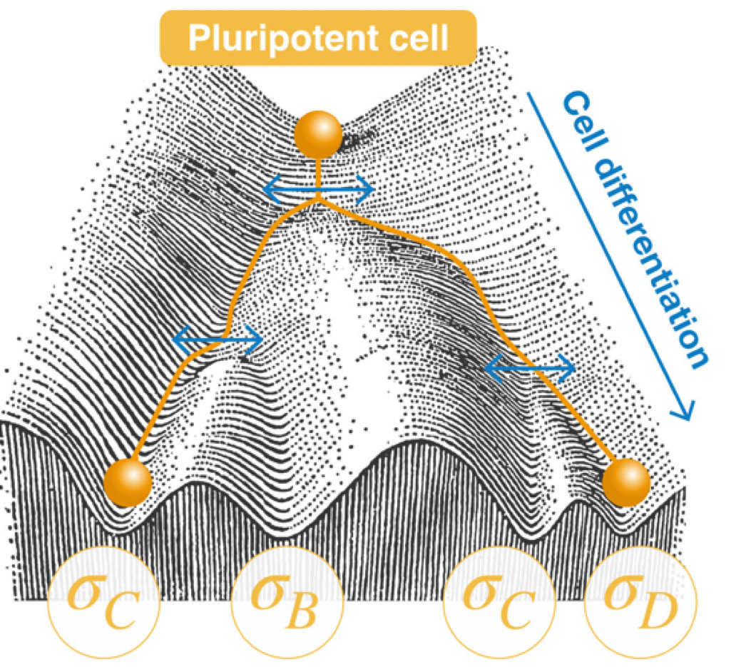
In cell-state theory in biology, cells transition between distinct stable states upon changing environmental cues [65, 89, 78]. When this occurs $\sigma$ values change accordingly, suggesting of a new class of cellular $\sigma$-landscapes where each NESS corresponds to a minimum associated to a different $\sigma$ value, Figure 17. The $\sigma$-landscapes are the NESS-equivalent of the free energy landscapes describing equilibrium conformations of molecular systems [102]. When a single cell changes state, also its energetic $\sigma$-map changes, maybe coherently across sub-cellular locations and scales, from the molecular to the cellular level. Besides $\sigma$-maps one might envision measuring negentropy $\sigma_{-}$-maps in living cells reflecting the energy and negentropy requirements at subcellular level. A paradigmatic analog of the $\sigma$-landscape is the Waddington landscape in developmental theory [46] where the different developmental stages of a cell correspond to different phenotypes with their inherent $\sigma$ values, Figure 17. Therefore $\sigma$ appears as a unique descriptor of the NESS cellular state and a step towards quantifying energetically Waddington developmental landscapes. $\sigma$-landscapes open a paradigm about biological matter, the possibility of monitoring how embryonic cells, cancer cells and other pathological cell states change by correlating phenotypical and $\sigma$ changes. Does $\sigma$ reflect the functional heterogeneity and plasticity of cell states [78] from normal to tumorigenic? Finally, let us add to such landscape the dead-equilibrium state characterized by $\sigma=0$, and let us envision perturbing a dead system inducing a transition to a non-zero finite $\sigma$ restoring back the living state. That would be thrilling.

Finally, heatomics powered by the VSR approach might find applications to modern societal energy-related challenges, from climate change to energetic needs by AI. One might envision measuring the local weather fluctuations, which together with VSR-based dynamical models of the atmosphere might permit to monitor climate’s energy power and its evolution. Experimental measurements of $\sigma$ at all scales are most needed to illuminate the relevance of heat power for life.

References

- [1] (2012) Experimental free-energy measurements of kinetic molecular states using fluctuation theorems. Nature Physics 8 (9), pp. 688–694. Cited by: §5.
- [2] (2023) Atkins’ physical chemistry. Oxford University Press. Cited by: §3.
- [3] (1992) A microcalorimetric study of human erythrocytes in stirred buffer suspensions. Thermochimica acta 205, pp. 87–97. Cited by: Figure 8, §6.2.
- [4] (2014) A critique of methods for temperature imaging in single cells. Nature methods 11 (9), pp. 899–901. Cited by: §6.2, §7.
- [5] (2021) Brain power. Proceedings of the National Academy of Sciences 118 (32), pp. e2107022118. Cited by: §4.1.
- [6] (2018) On the thermodynamic origin of metabolic scaling. Scientific Reports 8 (1), pp. 1448. External Links: Document Cited by: §2.
- [7] (2015) Thermodynamic uncertainty relation for biomolecular processes. Physical review letters 114 (15), pp. 158101. Cited by: §5.
- [8] (2018) A sensitive calorimetric technique to study energy (heat) exchange at the nano-scale. Nanoscale 10 (21), pp. 10079–10086. Cited by: §10, §6.
- [9] (2016) Broken detailed balance at mesoscopic scales in active biological systems. Science 352 (6285), pp. 604–607. Cited by: §5.
- [10] (1982) The thermodynamics of computation—a review. International Journal of Theoretical Physics 21 (12), pp. 905–940. Cited by: §8.1.
- [11] (2021) Excess and loss of entropy production for different levels of coarse graining. Physical Review E 104 (2), pp. 024140. Cited by: §10.
- [12] (2017) Hierarchical bounds on entropy production inferred from partial information. Journal of Statistical Mechanics: Theory and Experiment 2017 (9), pp. 093210. Cited by: §5.
- [13] (1983) Quantum tunnelling in a dissipative system. Annals of physics 149 (2), pp. 374–456. Cited by: §8.
- [14] (2017) Experimental measurement of binding energy, selectivity, and allostery using fluctuation theorems. Science 355 (6323), pp. 412–415. Cited by: §5.
- [15] (2020) Single-molecule diffusometry reveals no catalysis-induced diffusion enhancement of alkaline phosphatase as proposed by fcs experiments. Proceedings of the National Academy of Sciences 117 (35), pp. 21328–21335. Cited by: §10.
- [16] (2018) Mitochondria are physiologically maintained at close to 50 c. PLoS biology 16 (1), pp. e2003992. Cited by: §7.
- [17] (2024) Implication of thermal signaling in neuronal differentiation revealed by manipulation and measurement of intracellular temperature. Nature Communications 15 (1), pp. 3473. Cited by: §7.
- [18] (2017) Experiments in stochastic thermodynamics: short history and perspectives. Physical Review X 7 (2), pp. 021051. Cited by: §5.
- [19] (2014) Chemistry in motion: tiny synthetic motors. Accounts of chemical research 47 (12), pp. 3504–3511. Cited by: §11.
- [20] (2005) Verification of the crooks fluctuation theorem and recovery of rna folding free energies. Nature 437 (7056), pp. 231–234. Cited by: §5.
- [21] (2025) Thermodynamic dissipation constrains metabolic versatility of unicellular growth. Nature communications 16 (1), pp. 8543. Cited by: §1.
- [22] (2013) Non-equilibrium thermodynamics. Courier Corporation. Cited by: §5.
- [23] (2021) Improving thermodynamic bounds using correlations. Physical Review X 11 (4), pp. 041061. Cited by: §5.
- [24] (2026) Note: In preparation Cited by: §8.
- [25] (2024) Variance sum rule: proofs and solvable models. New Journal of Physics 26 (6), pp. 063013. Cited by: §6.1, §6, §8.2.
- [26] (2024) Variance sum rule for entropy production. Science 383 (6686), pp. 971–976. Cited by: §10, §10, §10, Figure 5, Figure 6, Figure 7, Figure 8, §6.1, §6.1, §6.2, §6.
- [27] (2022) Mathematical, thermodynamical, and experimental necessity for coarse graining empirical densities and currents in continuous space. Physical Review Letters 129 (14), pp. 140601. Cited by: §5.
- [28] (2010) Molecular driving forces: statistical thermodynamics in biology, chemistry, physics, and nanoscience. Garland Science. Cited by: §3.
- [29] (1937) The cosmological constants. Nature 139 (3512), pp. 323–323. Cited by: §9.
- [30] (2012) Mapping intracellular temperature using green fluorescent protein. Nano letters 12 (4), pp. 2107–2111. Cited by: §7.
- [31] (2014) Nucleic acid based fluorescent nanothermometers. Acs Nano 8 (10), pp. 10372–10382. Cited by: §7.
- [32] (2025) Macroscopic stochastic thermodynamics. Reviews of Modern Physics 97 (1), pp. 015002. Cited by: §5.
- [33] (2006) A master relation defines the nonlinear viscoelasticity of single fibroblasts. Biophysical journal 90 (10), pp. 3796–3805. Cited by: §6.1.
- [34] (2021) Following molecular mobility during chemical reactions: no evidence for active propulsion. Journal of the American Chemical Society 143 (49), pp. 20884–20890. Cited by: §10.
- [35] (2018) The statistical physics of active matter: from self-catalytic colloids to living cells. Physica A: Statistical Mechanics and its Applications 504, pp. 106–120. Cited by: §10.
- [36] (2016) How far from equilibrium is active matter?. Physical review letters 117 (3), pp. 038103. Cited by: §10.
- [37] (2021) Enzymes as active matter. Annual Review of Condensed Matter Physics 12 (1), pp. 177–200. Cited by: §8.1.
- [38] (2024) Viscoelastic phenotyping of red blood cells. Biophysical Journal 123 (7), pp. 770–781. Cited by: Figure 6, Figure 7, §6.1.
- [39] (2003) Bias and error in estimates of equilibrium free-energy differences from nonequilibrium measurements. Proceedings of the National Academy of Sciences 100 (22), pp. 12564–12569. Cited by: §5.
- [40] (2021) Entropy production fluctuations encode collective behavior in active matter. Physical Review E 103 (1), pp. 012613. Cited by: §10.
- [41] (2018) Diffusion measurements of swimming enzymes with fluorescence correlation spectroscopy. Accounts of chemical research 51 (9), pp. 1911–1920. Cited by: §10.
- [42] (2009) Artificial brownian motors: controlling transport on the nanoscale. Reviews of Modern Physics 81 (1), pp. 387–442. Cited by: §11.
- [43] (2020) Sub-nanowatt microfluidic single-cell calorimetry. Nature communications 11 (1), pp. 2982. Cited by: §10, §6.
- [44] (2020) Thermodynamic uncertainty relations constrain non-equilibrium fluctuations. Nature Physics 16 (1), pp. 15–20. Cited by: §5.
- [45] (2008) Stochastic gravity: theory and applications. Living Reviews in Relativity 11 (1), pp. 1–112. Cited by: §9.
- [46] (2012) The molecular and mathematical basis of waddington’s epigenetic landscape: a framework for post-darwinian biology?. BioEssays 34 (2), pp. 149–157. External Links: Document Cited by: §11.
- [47] (2020) Sub-nanowatt resolution direct calorimetry for probing real-time metabolic activity of individual c. elegans worms. Nature communications 11 (1), pp. 2983. Cited by: §10, §6.
- [48] (2020) Protein condensates as aging maxwell fluids. Science 370 (6522), pp. 1317–1323. Cited by: §11.
- [49] (2018) Catalytic enzymes are active matter. Proceedings of the National Academy of Sciences 115 (46), pp. E10812–E10821. Cited by: §10.
- [50] (2009) Recovery of free energy branches in single molecule experiments. Physical review letters 102 (7), pp. 070602. Cited by: §5.
- [51] (2017) Artificial molecular motors. Chemical Society Reviews 46 (9), pp. 2592–2621. Cited by: §11.
- [52] (2015) Modern thermodynamics: from heat engines to dissipative structures. John Wiley & Sons. Cited by: §3.
- [53] (2024) Motility of an autonomous protein-based artificial motor that operates via a burnt-bridge principle. Nature Communications 15 (1), pp. 1511. Cited by: §11.
- [54] (2013) Nanometre-scale thermometry in a living cell. Nature 500 (7460), pp. 54–58. Cited by: §7.
- [55] (2012) The energy–speed–accuracy trade-off in sensory adaptation. Nature physics 8 (5), pp. 422–428. Cited by: §1.
- [56] (1961) Irreversibility and heat generation in the computing process. IBM journal of research and development 5 (3), pp. 183–191. Cited by: §8.1.
- [57] (2008) Nano-calorimetry of small-sized biological samples. Thermochimica acta 477 (1-2), pp. 48–53. Cited by: §10, §6.
- [58] (2019) Quantifying dissipation using fluctuating currents. Nature communications 10 (1), pp. 1666. Cited by: §5.
- [59] (2024) Design and application of fluorescent probes to detect cellular physical microenvironments. Chemical reviews 124 (4), pp. 1738–1861. Cited by: §10, §6.
- [60] (2003) On the origin and the use of fluctuation relations for the entropy. Séminaire Poincaré 2, pp. 29–62. Cited by: §5.
- [61] (2008) Mean mass-specific metabolic rates are strikingly similar across life’s major domains: evidence for life’s metabolic optimum. Proceedings of the National Academy of Sciences 105 (44), pp. 16994–16999. External Links: Document Cited by: §2.
- [62] (2020) Inferring entropy production from short experiments. Physical review letters 124 (12), pp. 120603. Cited by: §5.
- [63] (2021) Thermodynamics of active field theories: energetic cost of coupling to reservoirs. Physical Review X 11 (2), pp. 021057. Cited by: §10.
- [64] (2015) Cell biology by the numbers. Garland Science. Cited by: §4.1.
- [65] (2021) Cell state transitions: definitions and challenges. Development 148 (20), pp. dev199950. Cited by: §11.
- [66] (2017) Entropy production in field theories without time-reversal symmetry: quantifying the non-equilibrium character of active matter. Physical Review X 7 (2), pp. 021007. Cited by: §10.
- [67] (1997) Mechanistic aspects of enzymatic catalysis: lessons from comparison of rna and protein enzymes. Annual review of biochemistry 66 (1), pp. 19–59. Cited by: §10.
- [68] (2025) Time-dependent trajectory of a one-dimensional gaussian non-markovian observable does not reveal its nonequilibrium character. Physical Review E 112 (1), pp. 014132. Cited by: §10.
- [69] (2013) Bioenergetics. Academic press. Cited by: §1, §8.1.
- [70] (2009) Fluorescence lifetimes: fundamentals and interpretations. Photosynthesis research 101 (2), pp. 181–194. Cited by: §6.
- [71] (2012) Intracellular temperature mapping with a fluorescent polymeric thermometer and fluorescence lifetime imaging microscopy. Nature communications 3 (1), pp. 705. Cited by: §7.
- [72] (2009) Entropy production and the arrow of time. New Journal of Physics 11 (7), pp. 073008. Cited by: §5.
- [73] (2021) Stochastic thermodynamics: an introduction. Princeton University Press. Cited by: §5.
- [74] (2024) Thermodynamic cost for precision of general counting observables. Physical Review E 109 (6), pp. 064128. Cited by: §10, §5.
- [75] (1956) The enthalpy change of adenosine triphosphate hydrolysis. Journal of Biological Chemistry 218 (2), pp. 945–959. Cited by: §8.1.
- [76] (2007) Viscoelasticity of the human red blood cell. American Journal of Physiology-Cell Physiology 293 (2), pp. C597–C605. Cited by: §6.1.
- [77] (2004) Fluorescence correlation spectroscopy with high-order and dual-color correlation to probe nonequilibrium steady states. Proceedings of the National Academy of Sciences 101 (9), pp. 2828–2833. Cited by: §5.
- [78] (2024) Establishing a conceptual framework for holistic cell states and state transitions. Cell 187 (11), pp. 2633–2651. Cited by: §11.
- [79] (2015) Universal axial fluctuations in optical tweezers. Optics Letters 40 (5), pp. 800–803. Cited by: §8.
- [80] (2012) Force spectroscopy with dual-trap optical tweezers: molecular stiffness measurements and coupled fluctuations analysis. Biophysical Journal 103 (9), pp. 1919–1928. Cited by: §8.
- [81] (2022) Molten globule–like transition state of protein barnase measured with calorimetric force spectroscopy. Proceedings of the National Academy of Sciences 119 (11), pp. e2112382119. Cited by: §5.
- [82] (2022) Stem–loop formation drives rna folding in mechanical unzipping experiments. Proceedings of the National Academy of Sciences 119 (3), pp. e2025575119. Cited by: §5.
- [83] (2002) A two-state kinetic model for the unfolding of single molecules by mechanical force. Proceedings of the National Academy of Sciences 99 (21), pp. 13544–13548. Cited by: §5.
- [84] (2008) Nonequilibrium fluctuations in small systems: from physics to biology. Advances in chemical physics 137, pp. 31. Cited by: §5.
- [85] (2025) Continuous-time random walk model for the diffusive motion of helicases. QRB discovery 6, pp. e26. Cited by: §10, §5.
- [86] (2021) Quantifying entropy production in active fluctuations of the hair-cell bundle from time irreversibility and uncertainty relations. New Journal of Physics 23 (8), pp. 083013. Cited by: §5.
- [87] (2012) Entropy production and kullback-leibler divergence between stationary trajectories of discrete systems. Physical Review E—Statistical, Nonlinear, and Soft Matter Physics 85 (3), pp. 031129. Cited by: §5.
- [88] (2024) Thermodynamic probes of life. Science 383 (6686), pp. 952–953. Cited by: §6.
- [89] (2022) Control of cell state transitions. Nature 609 (7929), pp. 975–985. Cited by: §11.
- [90] (2025) Why life is hot. arXiv preprint arXiv:2512.04725. Cited by: §11, §11.
- [91] (2025) What is life? the physical aspect of the living cell. Rare Treasure Editions. Cited by: §8.
- [92] (2012) Stochastic thermodynamics, fluctuation theorems and molecular machines. Reports on progress in physics 75 (12), pp. 126001. Cited by: §5.
- [93] (2024) Active colloids: from fundamentals to frontiers. Royal Society of Chemistry. Cited by: §10.
- [94] (2021) Improved bounds on entropy production in living systems. Proceedings of the National Academy of Sciences 118 (18), pp. e2024300118. Cited by: §5.
- [95] (2021) Harnessing dna for nanothermometry. Journal of biophotonics 14 (2), pp. e202000341. Cited by: §7.
- [96] (2025) Single molecule–driven nanomotors reveal the dynamic-disordered chemomechanical transduction of active enzymes. Science Advances 11 (5), pp. eads0446. Cited by: §10.
- [97] (2020) Exact coarse graining preserves entropy production out of equilibrium. Physical Review Letters 125 (11), pp. 110601. Cited by: §5.
- [98] (2018) Plug and play anisotropy-based nanothermometers. ACS Photonics 5 (7), pp. 2676–2681. Cited by: §7.
- [99] (2024) Fluorescence lifetime imaging microscopy. Nature Reviews Methods Primers 4 (1), pp. 80. Cited by: §6.
- [100] (2003) Molecular fluorescence lifetime fluctuations: on the possible role of conformational effects. Chemical physics letters 372 (1-2), pp. 282–287. Cited by: §10, §6.
- [101] (2010) Temperature sensing using fluorescent nanothermometers. ACS nano 4 (6), pp. 3254–3258. Cited by: §7.
- [102] (2008) Potential landscape and flux framework of nonequilibrium networks: robustness, dissipation, and coherence of biochemical oscillations. Proceedings of the National Academy of Sciences 105 (34), pp. 12271–12276. Cited by: §11.
- [103] (2019) Direct single molecule imaging of enhanced enzyme diffusion. Physical review letters 123 (12), pp. 128101. Cited by: §10.
- [104] (2021) Physical bioenergetics: energy fluxes, budgets, and constraints in cells. Proceedings of the National Academy of Sciences 118 (26), pp. e2026786118. Cited by: §1.
- [105] (2025) Viscoelastic mechanics of living cells. Physics of Life Reviews 53, pp. 91–116. Cited by: §6.1.
- [106] (2020) Advances and challenges for fluorescence nanothermometry. Nature methods 17 (10), pp. 967–980. Cited by: §7.