The Importance of Being Statistically Earnest:
A Critical Re-evaluation of GSM-Symbolic

Abstract

The GSM-Symbolic benchmark (Mirzadeh et al., 2025) reported consistent performance drops across 25 Large Language Models (LLMs) when tested on template-generated variants of GSM8K problems, concluding that the models lack genuine reasoning capabilities. We argue that this conclusion rests on shaky statistical ground. Re-evaluating 20 open-weight models using Generalised Linear Mixed Models with per-question random effects, we find that only half exhibit statistically significant performance changes under the original prompt format. Moreover, we identify a previously unacknowledged factor: the main GSM-Symbolic dataset contains a systematically shifted distribution of larger integers in problem texts relative to GSM-Base (K-S statistic = 0.12, p < 0.001), contradicting the original authors’ claims. Controlling for this large number effect accounts for significance in roughly half the remaining cases. Among models with statistically significant performance deltas, we identify distinct, model-specific failure profiles - including fragility of variable binding, arithmetic limitations, and dual-task interference - underscoring that blanket claims about LLM reasoning are both statistically premature and mechanistically misleading.

The Importance of Being Statistically Earnest:
A Critical Re-evaluation of GSM-Symbolic

Dominika Długosz^1,2, Arlindo Oliveira¹, Natalia Díaz-Rodríguez^{2 1}Instituto Superior Técnico & INESC-ID, Universidade de Lisboa, Portugal ²Dept. of Computer Science and AI & DaSCI Institute, Universidad de Granada, Spain Correspondence: dominika.dlugosz@tecnico.ulisboa.pt

1 Introduction

As Large Language Models (LLMs) are developed towards increased robustness in reasoning, reliable evaluation of their problem-solving capabilities is becoming instrumental. Several benchmarking datasets have been proposed to facilitate principled assessment of LLMs, including GSM-Base - a dataset of 8.5k mathematical problems at grade school level (Cobbe et al., 2021).

However, as new models are released, they might be exposed to the publicly available benchmarking datasets, causing data contamination and possibly inflating the reported performance. Evaluating data contamination effects was the motivation behind the GSM-Symbolic study (Mirzadeh et al., 2025). The researchers extracted 100 questions from the GSM8K benchmark and, using carefully constructed templates to vary names and numbers involved, prepared 50 new variants of each of these questions, creating a dataset of 5000 examples. Having tested 25 models of varying architectures and sizes on the dataset, the authors observed a consistent performance decline on the new variants compared to the original 100 questions and hypothesised that this result demonstrates limitations in logical reasoning capabilities of LLMs.

In this work, we revisit the GSM-Symbolic study to quantitatively assess the extent of the reported deterioration and provide more insights concerning possible failure mechanisms. Our re-evaluation reveals that the per-model accuracy deltas often fail to reach statistical significance ($p<0.05$) when subjected to rigorous hypothesis testing. Furthermore, focusing on the models which do exhibit significant performance changes, we propose alternative prompt formats to help isolate potential contributing factors: reliance on the exact strings of words from the GSM8K questions (as assumed by Mirzadeh et al.), difficulties in object attribute tracking, and limitations of arithmetic nature.

2 Related Work

Despite long-standing calls for rigorous hypothesis testing in Natural Language Processing (NLP) evaluation (Marie et al., 2021; Dror et al., 2018), the absence of statistical significance testing remains a persistent methodological concern. Arias et al. (2025) observed a declining trend in the use of statistical validation of evaluations of LLM-generated text over the 2022-2024 period. Vaugrante et al. (2024)’s reevaluation of several advanced prompting techniques revealed a general lack of statistically significant differences when compared to the respective baselines. The authors suggest that the field might be approaching a replication crisis, mirroring similar historical occurrences in psychology (Simmons et al., 2011; Collaboration, 2015) and medicine (Ioannidis, 2005; Begley and Ellis, 2012).

First described by Clark (1973), the language-as-fixed-effect fallacy is a type of statistical error known in psychological and linguistic research, referring to treating specific language materials as fixed rather than random effects. By ignoring the inherent, idiosyncratic variance between individual linguistic items (e.g. particular words or sentences), researchers risk making broad claims about language processing that are actually false positives driven by the specific sample used. To mitigate this fallacy, the field has shifted to mixed-effect modelling of the experimental results (Baayen et al., 2008), e.g. through Generalised Linear Mixed Models (GLMM) (Jaeger, 2008). GLMMs extend generalised linear models (e.g. logistic regression) by incorporating both fixed effects - population-level factors of theoretical interest - and random effects that capture variability across items or subjects, enabling statistically valid inference over heterogeneous, non-independent data. More recently, Van Der Lee et al. (2019) and Card et al. (2020) argued for adopting mixed models in the fields of Natural Language Processing and Generation.

Reliable evaluation of logical and mathematical reasoning capabilities of LLMs has been the motivation behind multiple benchmarks, such as MATH Hendrycks et al. (2021), BIG Bench HARD (Suzgun et al., 2023), FrontierMath (Glazer et al., 2024), or the subject of the current study, GSM8K (Cobbe et al., 2021) with several descendants,

including GSM-Symbolic (Mirzadeh et al., 2025), GSM-Plus (Li et al., 2024), GSM-Identity (Negi et al., 2026), and GSM-Ranges (Shrestha et al., 2025). However, systematic evaluation of LLMs poses a number of challenges, rendering the interpretation and generalisability of the results more nuanced. As demonstrated by Sclar et al. (2023), LLMs display high sensitivity to prompt formatting, with surface-level modifications linked to potentially vast changes in performance independently of difficulty of the problem to be solved. The effect seems to be independent of model family or scale (Sclar et al., 2023; Alhetelah and Ahmad, 2026), with changes as trivial as letter case or separator swap drastically changing models’ outputs Errica et al. (2025). Due to impracticality of manual analysis, benchmarks frequently expect strict formatting of the answers. However, literature suggests that formatting constraints may induce a cognitive load collapse (particularly in smaller models), leading to not just incorrect answers, but a complete failure to handle the problems (Cazares, 2026; Mittal, 2026). Furthermore, number processing in LLMs is sensitive to tokenisation mechanisms used (Spathis and Kawsar, 2024; Singh and Strouse, 2024). Models struggle to generalise their arithmetic capabilities to larger numbers, expressing which requires more digits (Yang et al., 2023; Zhou et al., 2024) - an issue resulting in recent argumentation for single-token number embeddings (Kreitner et al., 2025; Zhou et al., 2025). Approaches such as Program of Thought (Chen et al., 2023) and Program-Aided Language Models Gao et al. (2023b) attempt to circumvent the large-number limitations through instructing models to generate Python code from which the final numerical answer is calculated using an external interpreter. However, as demonstrated by Shrestha et al. in their high-number-range adaptation of the GSM8K benchmark, offloading the calculations to an external tool might not be sufficient as higher values frequently deteriorate the underlying reasoning processes of a model.

3 Methodology

This section details the experimental setup underlying our re-evaluation. We begin by defining the datasets, metrics, and models used (Sections 3.1–3.2), before describing the prompt formats designed to probe candidate failure modes (Section 3.3). We then introduce a large number effect metric to separate arithmetic difficulty from reasoning failures per se (Section 3.4), and describe the statistical framework — based on GLMMs with per-question random effects — used to assess significance of the observed effects (Section 3.5). Finally, Section 3.6 presents the research questions and experimental design. The code developed for all experiments and evaluations performed in the scope of this project is available at https://github.com/the-mysh/gsm-symbolic-benchmarking.

3.1 Definitions

Datasets

Our experiments focus on two datasets from the GSM-Symbolic study (Mirzadeh et al., 2025): GSM-Variants (labelled as main or Symbolic in the study), i.e. the 5000 template-generated questions; and GSM-Base (GSM8K 100 in Mirzadeh et al.), i.e. the corresponding 100 originals chosen from Cobbe et al.. A question from the GSM-Base dataset and its 50 variants from GSM-Variants share the same integer template ID. We refer to the phenomenon of decreased accuracy on GSM-Variants questions (w.r.t. to performance GSM-Base problems) as the variant effect.

Metrics

Across the paper, we express average accuracy as a percentage of correctly answered questions. Accuracy deltas (differences in accuracy between two datasets) are expressed in percentage points (pp). We use the term variant performance delta to describe raw change in accuracy, in percentage points, from GSM-Base to GSM-Variants datasets: $\Delta_{var}=\overline{A}_{GSM-Base}-\overline{A}_{GSM-Variants}$. The accuracies ($\overline{A}$) in this context are averaged across the entire respective datasets.

3.2 Models

The GSM-Symbolic study evaluated the performance of 25 LLMs. For economical and practical reasons, we exclude the four proprietary models (all developed by OpenAI) from our analysis. In addition, we omit Phi-3-small-128k-instruct (Microsoft) due to technical difficulties. Otherwise, we follow the original list, presenting 20 open-weight models for our experiments. The models and limitations can be consulted in Appendix B.

3.3 Prompt Formats and Failure Modes

Throughout the work and in accordance with the GSM-Symbolic study, we use 8-shot prompting with the standard GSM8K shots (Gao et al., 2023a), where a shot is a single mathematical problem with a step-by-step solution. First, we reproduce the GSM-Symbolic results using the original prompt format, which we refer to as GSM prompt. In later experiments (see Section 3.6), we modify the solutions to the eight example problems alongside with the prompt introduction line. The exact templates of all prompts used in our experiments, described below, are included in Appendix C.

To test whether the models indeed rely on the exact phrasing of the original GSM prompt, we propose a simple rewording of the original answers. We remove the explicit instruction to follow a stepwise approach, but include step introduction phrases (First, calculate…, Next, …, etc.) where their relevance is justified by the problem structure. We refer to this prompt format as simple natural language (NL) prompt.

Solving grade school problems exemplified by GSM8K requires robust variable binding and internal state tracking. To isolate the fragility of these capabilities as the possible factors contributing to the variant effect, we propose a structured NL prompt. In addition to the modified phrasing of the simple NL prompt, we include explicit sections with headers: Given, To find, and Solution, detailing all the relevant quantities in the first section and re-stating the calculation target in the second. By introducing these more rigid formatting constraints, we aim to provide a supportive scaffolding, partially offloading the cognitive capabilities to the introduced structure. On the other hand, as discussed before, strict formatting requirements could be a factor negatively influencing performance of smaller models (Cazares, 2026; Mittal, 2026).

Finally, we adapt the example answers into two types of code prompts, where the model is asked to provide a valid Python function accepting no arguments, performing the necessary calculations using variables defined inside the function, and returning the calculated result. With these prompts, we aim to investigate arithmetic processing as the potential source of the variant effect. Analogously to the NL prompts described above, we propose two code prompts: a structured code prompt following the same three-part structure as the structured NL prompt, and a simple code prompt, which maximally limits any additions over the standard short explanations of steps taken to solve the problems.

Answers from experiments using the GSM, simple NL, and structured NL prompts are extracted using standard pattern matching: we first attempt to match the target response line (The final answer is) is followed by a number; if this fails, we extract the last number in the response, following GSM-Symbolic. For the code prompts, we attempt to execute the output function via a Python interpreter after safety checks, collecting error type information for non-executing outputs (Appendix E).

3.4 The Effect of Large Numbers

We believe it is imperative to separate purely arithmetic difficulties from limitations of mathematical reasoning understood as a process of constructing logically consistent solution procedures, grounded in context and common sense. To this end, we evaluate whether larger numbers in problems’ texts are a predictor of altered performance. We construct a large number effect metric, denoted as $\gamma$ reflecting the total digit load of a question. For each question, we extract all numerically expressed integers (i.e. we ignore cases such as ’three’, ’twice’, ’half’, and all numerically expressed fractions). We then compute logarithms of base 10 for each number (negative numbers, if any, are taken at their absolute value; for 0, we take the value of 1) and sum the obtained values for a given question. For a given question,

$$\gamma=\sum_{n\in\mathcal{N}}log(n)$$ (1)

where $\mathcal{N}$ - set of all numerically expressed integers in the question text. This metric captures two effects: firstly, the logarithm assigns unit growth for each added digit, accounting for the number-splitting effect in tokenisation; secondly, larger numbers are expected to appear less in training data and therefore errors in arithmetic operations involving these numbers can be deemed more likely.

We test for this large number effect on combined data from both GSM-Variants and GSM-Base datasets, separately for each LLM. We assess two aspects: (1) whether the large number effect is present (i.e. whether larger numbers are associated with decreased performance); (2) whether, controlling for the number magnitude, variant effect remains significant. The details of the test setup are discussed in Section 3.5. When fitting the statistical model, we use centre $\gamma$ to zero mean; we denote the centred metric as $\gamma_{c}$.

3.5 Statistical Significance Testing

We model the influence of the different factors on response accuracy using a GLMM. We use a binomial family with logit link, appropriate for the binary correct/incorrect outcome. The choice of the model (GLMM) allows accounting for the non-independence of repeated observations - results for the same question template should not be treated as statistically independent.

We define two instances of the model. With GLMM 1, we model the binary outcome $Correct$ - whether a given question was solved correctly by a given LLM - as a function of question type ($Variant$: 0 for GSM-Base, 1 for GSM-Variants) as a fixed effect, with a random intercept (baseline difficulty) per template ($Id$). The random intercept accounts for the fact that GSM-Base questions and their GSM-Variants share the same underlying template, making their responses non-independent; it allows the baseline difficulty to vary freely across templates rather than assuming all questions are equally hard. The fixed effect of $Variant$ then estimates whether belonging to the variant set is associated with a reliable change in accuracy, over and above this template-level variability. In Wilkinson notation Wilkinson and Rogers (1973); Bates et al. (2015), GLMM 1 is specified as follows:

$$Correct\sim Variant+(1|Id)$$ (2)

Next, we extend GLMM 1 by including the centred large number effect metric $\gamma_{c}$ (see Section 3.4) - as a second fixed effect. This yields GLMM 2:

$$Correct\sim Variant+\gamma_{c}+(1|Id)$$ (3)

where the estimate for $\gamma_{c}$ tests whether numeric load is independently associated with accuracy, and the estimate for $Variant$ - whether the variant effect persists after controlling for it - since questions from GSM-Variants may differ from their GSM-Base counterparts not only in surface form but in the numerical values they employ.

We fit both models separately for each LLM (see Section 3.2) and prompt format (see Section 3.3). We perform the fitting using a Python library pymer4 Jolly (2018), wrapping over R’s LME4 Bates et al. (2015). We report the obtained fixed-effect estimates as odds ratios (OR). OR > 1 indicates increased odds of a correct response relative to baseline, OR < 1 decreased odds. In figures, we report log ORs for visual symmetry around zero. The P values corresponding to the estimates serve as an indication of statistical significance of each of the effects.

Note: to evaluate the global significance of the variant and large number effects across all models, we apply the Holm-Bonferroni correction across the evaluated LLMs, separately per effect. We select this over the standard Bonferroni procedure as it offers superior statistical power while maintaining strict control over the family-wise error rate, ensuring that our critique does not unfairly penalize marginal but real effects. We nonetheless report and discuss uncorrected p-values alongside corrected ones, as our primary interest lies in model-specific failure profiles rather than family-wise conclusions.

3.6 Research Questions and Experiments

We consider three principal research questions.

RQ1. Does the variant effect reported by the GSM-Symbolic study exhibit statistical significance under GLMM?

RQ2. What are the possible failure modes responsible for the observed performance decline?

RQ3. Are models sensitive to larger numbers in the range used in the GSM-Base and GSM-Variants datasets of GSM-Symbolic?

To answer RQ1, we reproduce the GSM-Symbolic experiments (Ex1; model limitations in Section 3.2), fitting GLMM 1 (Section 3.5) per LLM and comparing P values against $\alpha=0.05$ to evaluate statistical significance of the variant effect.

For RQ2, models significant under Ex1 are evaluated on the four alternative prompt formats (Ex2.A–D: simple NL, structured NL, simple code, and structured code prompts - see Section 3.3), using GLMM 1 per LLM and prompt format to assess whether the variant effect vanishes.

For RQ3, we reuse raw model evaluation data from Ex2.A to Ex2.D in corresponding experiments Ex3.A to Ex3.D. We fit GLMM 2 (see Section 3.5) to combined GSM-Variants and GSM-Base results (per LLM and prompt format) to evaluate the statistical significance of the large number effect, as well as the residual significance of large-number-effect-corrected variant effect.

4 Results

In this section, we present the results of our experiments: evaluating statistical significance of results presented in Mirzadeh et al. (2025) and investigating possible underlying causes of the reported performance decline.

4.1 Reproduction of GSM-Symbolic

Figure 1: Reproduction of the GSM-Symbolic benchmark. Top: odds ratios and confidence intervals obtained using the GLMM; dashed vertical line marking the null-effect (i.e. OR = 1). Bottom left: variant performance deltas ($\Delta_{var}$) in percentage points (pp). Bottom right: P values (prior to Holm-Bonferroni correction); dashed vertical line marking the standard statistical significance threshold $\alpha=0.05$.

Results of Ex1 are illustrated in Figure 1. Full details are included in Tables 2 and 3 in Appendix D. Out of 20 models subjected to GLMM evaluation, 10 show statistically significant variant effect when considered individually. For gemma-2-2b, we observe a degenerate result, for which we provide additional analysis in Appendix D.3.

4.2 Alternative Prompt Formats

Detailed results for the four alternative prompt formats (Ex2.A - Ex2.D) are shown in Appendix D.2. For four of the LLMs, the variant effect is rendered statistically insignificant on all four alternative prompt formats. These models are: Phi-3.5-mini-instruct, gemma-2-9b, Mathstral-7B-v0.1, and Mistral-7B-Instruct-v0.1. In further analysis, we focus on the remaining six models, for which we observe a significant variant effect with at least one of the new prompt formats: gemma-2b, gemma-2-2b, gemma-7b-it, phi-2, Meta-Llama-3-8B-Instruct, and Meta-Llama-3-8B-Instruct. The dynamics of the variant effect for these models are shown in a Figure 2. Note: for gemma-2-2b, we again observe degenerate GLMM estimates with the structured NL prompt and structured code prompt.

Figure 2: Accuracies and and accuracy changes (variant performance delta ($\Delta_{var}$, see Section 3.1) across the five prompt formats (see Section 3.3), for six example LLMs (see Section 4.2). Hatching in the bottom plot indicates the given variant effect is not significant (p > .05, prior to the Holm-Bonferroni correction).

4.3 The Large Number Effect

Figure 7 in Appendix D.4 presents the distributions of numerically expressed integers extracted from questions of the GSM-Base and GSM-Variants dataset of the GSM-Symbolic benchmark. To formally confirm the visible systematic shift towards larger numbers in GSM-Variants, we conduct a two-sample Kolmogorov-Smirnov test on the unrolled occurrences in both datasets. The test confirms a highly statistically significant difference between the underlying distributions ($D=0.1201$, $p<0.001$). This result contradicts the cursory assessment made in one of the ablation studies of the GSM-Symbolic paper (Ablation: The Impact of Arithmetic Accuracy, Appendix A.6), where the authors stated: “overall, the range of numbers does not increase significantly” (Mirzadeh et al., 2025).

The results of experiments E3.A to Ex3.D, i.e. of our evaluation of the large number effect on model performance, are shown in Table 14 and Figure 8 in Appendix D.4. As demonstrated by these results, large numbers are a predictor of decreased performance on pooled GSM-Base and GSM-Variants questions for 6 of the models with the canonical GSM prompt, 8 models with the simple NL prompt, and 7 with the structured NL one. Either of the code prompts removes the significance of the large number effect, except in the case of gemma-2-2b model on the structured code prompt.

The test for residual significance of the variant effect, accounting for the large number effect, yields mixed results - as shown in Table 15 in Appendix D.4. In just over 50% of cases, the significance of performance delta disappears under the correction. This is the case for Phi-3.5-mini-instruct, Mathstral-7B-v0.1, Meta-Llama-3-8B-Instruct, gemma-7b-it, and Mistral-7B-Instruct-v0.1 (5/10 cases) with GSM prompt; phi-2 (1/2) with simple NL prompt; Meta-Llama-3-8B-Instruct and gemma-2-2b (2/3) with the structured NL prompt; gemma-7b-it and Meta-Llama-3-8B (2/2) with the simple code prompt; and none (0/1) with the structured code prompt. In the remaining 8 instances, the residual variant effect persists despite the large number effect correction.

5 Discussion

We discuss the implications of our findings concerning the statistical standards of LLM evaluation and model-specific failure profiles.

5.1 The Importance of Statistics

Mirzadeh et al. argue that the observed drop in performance on template versions GSM8K problems indicates lack of genuine reasoning capabilities in the affected models and by extension, in LLMs of the time. Our results suggest that this conclusion might be premature. The variant effect is strikingly less prevalent a phenomenon than implied in the GSM-Symbolic study. On the contrary, we demonstrate that only 10 of the 20 models we re-evaluate display statistically significant variant effect.

Furthermore, our analysis based on the models which individually (pre-correction) exhibit significant variant effect suggests that the influence of number distribution shift should not be ignored when interpreting results of GSM-Symbolic. While sensitivity to large numbers is indubitably an issue to be considered, failures due to arithmetic capabilities should not, in our opinion, be classified as reasoning errors.

5.2 The Failed Estimate

Appendix D.3, contains an analysis for the degenerate fits observed across three prompt formats (GSM prompt, structured NL prompt, and structured code prompt) for gemma-2-2b. The model shows a consistent small-to-moderate variant effect (log OR $\approx$ 0.3 across formats) but standard errors cannot be reliably computed likely due to numerical issues in Hessian inversion, themselves a consequence of the sparse binary data structure. We therefore exclude this model from further analysis.

5.3 Case Study of Failure Modes

While the variant effect may be indicative of data contamination in the affected models, our results suggest that the underlying failure mechanisms vary. Our analysis reveals several likely phenomena - behaviourally-motivated hypotheses subject to further verification through mechanistic interpretability techniques - described below.

Fragility of variable binding

For gemma-2b, the variant effect remains significant under simple rewording of the example solutions (simple NL prompt), but vanishes when the structured NL prompt is used. As discussed, the supportive scaffolding introduced by this prompt likely offloads the difficult (for the model) tasks of associating values with objects and tracking the resulting internal state to the external scratch pad of the generated response.

Limited arithmetic capabilities

For phi-2, variant effect remains significant across the NL prompt adaptations, but disappears entirely with the code prompts, where the otherwise significant large number effect also vanishes. For Phi-3.5-mini-instruct and Mistral-7B-Instruct-v0.1, for which the variant effect vanishes with all proposed prompt adaptations, the drop in accuracy on the GSM prompt can be fully explained by sensitivity to large numbers. For these models, arithmetic capabilities - and not lack of reasoning - seem to be the primary factor contributing to the variant effect.

Reliance on learnt patterns

Models gemma-2-9b and Mathstral-7B-v0.1 also exhibit the variant effect only with the original GSM prompt, but unlike the aforementioned Phi-3.5-mini and Mistral-7B-Instruct, are fully or partly immune to the number effect - possibly owing to the larger capacity (Gemma with 9B parameters) or training specific for mathematical reasoning (Mathstral). For these two models, we do not find an explanation for the original variant effect other than replication of patterns learnt from training data.

Dual-task interference

For Meta-Llama-3-8B, NL perturbations (simple NL prompt, structured NL prompt) are associated with a strong decrease in accuracy and, as shown in Fig. 9, a large number of empty answers. This behaviour can be interpreted in terms of dual-task inference, mirroring a phenomenon known in psychology Pashler (1994). Attempting to follow out-of-distribution formatting requirements while simultaneously solving a mathematical problem, the model fails at both tasks. Similar effects on a smaller scale seem to occur for two other models, in each case under different conditions. For Meta-Llama-3-8B-Instruct, the variant effect resurfaces on the structured NL prompt; on the other hand, with the structured code prompt, offloading the arithmetic operations to an external tool appears sufficient to counter-balance the effect of length or strict formatting. For gemma-7b-it, the picture is reverted, but describing a similar underlying mechanism; following the requirements of code syntax exhausts the working memory, leading to significant variant effect on simple code prompt. However, supportive scaffolding introduced by the structured NL prompt appears to restore the model’s relative performance.

Overall, our results demonstrate the diversity of possible root causes for failures on reasoning benchmarks and highlight the inappropriateness of blanket statements when analysing the outcomes.

6 Conclusions

This work presents a re-evaluation of the GSM-Symbolic benchmark, and its primary message is methodological: claims about the reasoning capabilities - or incapabilities - of LLMs demand statistical rigour. The widespread absence of significance testing in LLM evaluation is not merely an academic concern; it shapes research agendas, informs policy, and influences public understanding of AI systems.

Our results challenge the central claim of Mirzadeh et al. (2025). Applying GLMM with appropriate random effects for item-level variability, we find that the variant effect is statistically significant for only 10 of 20 re-evaluated models. For the models showing significance pre-correction, we demonstrate that a systematic shift towards larger integers in the main GSM-Symbolic dataset constitutes a previously overlooked confound, partially or fully explaining the decline in several cases.

Crucially, for models whose variant effect proves robust to prompt perturbations, no single failure mode prevails. Instead, we observe a diverse landscape: limitations in arithmetic capabilities, fragile variable binding, and dual-task interference - the compounding of out-of-distribution entity processing with rigid structural constraints. Only three of the LLMs seem to purely rely on patterns learnt from their training data. The heterogeneity of the results underscores the importance of careful, case-based investigation, possibly supported by mechanistic understanding, in evaluating or speculating about cognitive capabilities of LLMs. We hope this work contributes to a more epistemically careful discourse around LLM evaluation, one that treats statistical validation not as an optional refinement, but as a prerequisite for credible claims.

Limitations

While our re-evaluation provides a statistically rigorous perspective on the GSM-Symbolic benchmark, our methodology has several constraints that invite further investigation.

Simplification of the large number effect metric

The metric we introduce to quantify arithmetic difficulty ($\gamma$, see Section 3.4) acts as a proxy for total number load. However, it only captures the magnitude of integers present in questions. It does not account for the presence of fractions, decimals, the complexity of specific arithmetic operations (e.g., carrying over in addition, division by primes), or the nuances of model-specific tokenization boundaries, all of which are known to impact arithmetic performance. Our chosen heuristics offers a balance between capturing two major expected confounds and the overall clarity of presentation (i.e. a single, expressive metric for the discussed class of numerical issues). Further work could devise individual metrics isolating the possible contributing effects.

Granularity of prompt perturbations

For models such as Phi-3.5-mini-instruct, gemma-2-9b, Mathstral-7B-v0.1, and Mistral-7B-Instruct-v0.1, the variant effect vanishes under all tested prompt variations. While we interpret this as a heavy reliance on superficial pattern matching, we cannot rule out extreme sensitivity to formatting. Further studies utilizing small-scale perturbations are required to isolate pattern matching from general format fragility.

Behavioural abstraction of cognitive mechanisms

Our hypotheses regarding working memory exhaustion, dual-task interference, and the fragility of variable binding are inferred from black-box behavioural evaluations. While these cognitive aspects align with the observed performance deltas across structured versus programmatic prompts, validating the exact root causes of these failures would require white-box interpretability techniques, such as activation patching or circuit tracing, to map how specific attention heads route out-of-distribution entities.

Scope of evaluated models

For practical and economic reasons, our evaluation is restricted to open-weight models, all under 30 billion parameters. We excluded frontier proprietary models. Moreover, with reproduction of the GSM-Symbolic study as our primary motivation, we do not include more recent LLMs. Consequently, our findings regarding format sensitivity and the statistical insignificance of the variant effect may not fully generalize to the state-of-the-art models that typically define upper-bound reasoning capabilities. However, the methodological critique, emphasising the necessity of statistical significance testing with appropriate tools and of controlling for dataset distribution shifts, applies universally to all models evaluated on this benchmark.

Ethical Considerations

Epistemological responsibility and AI discourse

This work challenges definitive claims regarding the presence or absence of “genuine reasoning” capabilities in Large Language Models. We emphasise the ethical necessity of rigorous statistical validation before making broad assertions about AI capabilities. Prematurely concluding that models lack reasoning abilities - or conversely, overestimating their abilities based on contaminated benchmarks - can misinform public understanding, guide flawed policy decisions, and skew future safety research. Our findings advocate for a more nuanced, statistically grounded discourse regarding model evaluation.

Use of cognitive metaphors

Throughout this paper, we employ terminology derived from cognitive science and psychology, such as “working memory”, “cognitive load”, and “dual-task interference”. We explicitly state that these terms are used as functional metaphors to describe mechanistic and architectural phenomena within LLMs, such as variable binding and internal state tracking. Their use is intended to provide an intuitive framework for understanding failure modes, and should not be interpreted as an assertion that these models possess human-like sentience, biological cognition, or consciousness.

Computational and environmental cost

We acknowledge the environmental impact associated with our experimental methodology. Re-evaluating the GSM-Symbolic benchmark required running inference across 20 distinct LLMs on thousands of prompt variations. While this incurs a notable compute and carbon footprint, we believe this cost is justified by the critical need to validate high-impact benchmark results and prevent a potential replication crisis within the Natural Language Processing community.

Use of AI assistance

In this work, we used the assistance of AI chat bots (Claude, Gemini) to identify the relevant sources cited across the article and in particular those mentioned in the Related Work section, as well as to help with concise phrasing of the text. In addition, coding agents (GitHub Copilot) were employed to help construct model evaluation, data analysis, and visualisation scripts.

Appendix

Appendix A Artifacts

A.1 Software and Infrastructure

Model inference and evaluation pipelines were implemented in Python utilizing the PyTorch framework (Paszke et al., 2019) and the Hugging Face transformers library (Wolf et al., 2020), alongside datasets (Lhoest et al., 2021) for benchmark data management. Data manipulation and preprocessing were conducted using pandas McKinney (2010) and numpy Harris et al. (2020).

All statistical hypothesis testing, including the formulation of GLMMs, was executed using pymer4 Jolly (2018) - which interfaces with the R lme4 package Bates et al. (2015) - as well as scipy Virtanen et al. (2020) and statsmodels Seabold and Perktold (2010). Visualizations were generated relying on matplotlib Hunter (2007) and seaborn Waskom (2021).

A.2 Computational Experiments

The evaluations were performed on NVIDIA A40 and NVIDIA V100 GPUs. The total computational budget required to run the full evaluation pipeline across all 20 models and prompt variations is estimated at approximately 1,000 GPU hours. The evaluated open-weight models range in size from 2 billion to 27 billion parameters, with exact model versions and sizes specified in Appendix B.

A.3 Artifact Licences and Terms of Use

The artifacts utilized in this study are publicly available for research purposes. The GSM8K dataset (Cobbe et al., 2021) is distributed under the MIT licence and the GSM-Symbolic benchmark (Mirzadeh et al., 2025) - under CC-BY-NC-ND 4.0. The evaluated Large Language Models are subject to their respective open-weight licenses: models from the Mistral and Mathstral families are released under the Apache 2.0 License; the Microsoft Phi models are released under the MIT License; the Google Gemma models are governed by the Gemma Terms of Use; and the Meta-Llama-3 models are governed by the custom Meta Llama 3 Community License. All third-party software packages and libraries used for inference and statistical analysis (e.g., PyTorch, Hugging Face transformers, pymer4) are open-source and utilized in accordance with their respective permissive licenses (primarily MIT, BSD, and Apache 2.0). All models, datasets, and software were used strictly for research and evaluation purposes. The custom evaluation code and data analysis scripts developed for this study will be released under the MIT License upon publication to facilitate reproducibility.

Appendix B Model Specifications

In our experiments, we use models downloaded from the Hugging Face repository (Wolf et al., 2020). Table 1 lists the models we evaluate together with the corresponding checkpoints (commit ids) for reproducibility. When reporting the results throughout the paper, we omit model family names for brevity.

Model	Commit ID	Parameters
google/gemma-2b	9cf48e52b224239de00d483ec8eb84fb8d0f3a3a	2B
google/gemma-2b-it	96988410cbdaeb8d5093d1ebdc5a8fb563e02bad	2B
google/gemma-7b	ff6768d9368919a1f025a54f9f5aa0ee591730bb	7B
google/gemma-7b-it	9c5798d27f588501ce1e108079d2a19e4c3a2353	7B
google/gemma-2-2b	c5ebcd40d208330abc697524c919956e692655cf	2B
google/gemma-2-2b-it	299a8560bedf22ed1c72a8a11e7dce4a7f9f51f8	2B
google/gemma-2-9b	33c193028431c2fde6c6e51f29e6f17b60cbfac6	9B
google/gemma-2-9b-it	11c9b309abf73637e4b6f9a3fa1e92e615547819	9B
google/gemma-2-27b-it	aaf20e6b9f4c0fcf043f6fb2a2068419086d77b0	27B
microsoft/phi-2	810d367871c1d460086d9f82db8696f2e0a0fcd0	2.7B
microsoft/Phi-3-mini-128k-instruct	f3c06aed622e14ca0abf5115094e4fc9a9948f36	3.8B
microsoft/Phi-3-medium-128k-instruct	a088b37c71d441ab6d862bb3fcfe6165b3014702	14B
microsoft/Phi-3.5-mini-instruct	2fe192450127e6a83f7441aef6e3ca586c338b77	3.8B
mistralai/Mistral-7B-v0.1	27d67f1b5f57dc0953326b2601d68371d40ea8da	7B
mistralai/Mistral-7B-Instruct-v0.1	ec5deb64f2c6e6fa90c1abf74a91d5c93a9669ca	7B
mistralai/Mistral-7B-v0.3	caa1feb0e54d415e2df31207e5f4e273e33509b1	7B
mistralai/Mistral-7B-Instruct-v0.3	c170c708c41dac9275d15a8fff4eca08d52bab71	7B
mistralai/Mathstral-7B-v0.1	ec3a48484ef241dfe03282edcb0f25e564923823	7B
meta-llama/Meta-Llama-3-8B	8cde5ca8380496c9a6cc7ef3a8b46a0372a1d920	8B
meta-llama/Meta-Llama-3-8B-Instruct	8afb486c1db24fe5011ec46dfbe5b5dccdb575c2	8B

Table 1: Models used in the experiments with Hugging Face checkpoints (commit ids) and parameter counts.

Models from the GSM-Symbolic paper which were omitted in the current study:

• microsoft/Phi-3-small-128k-instruct

• gpt-4o-mini

• gpt-4o

• o1-mini

• o1-preview

We did not evaluate closed models (GPT-4o, o1) because of technical and economical constraints. For microsoft/Phi-3-small-128k-instruct, configuring Flash Attention on our hardware proved impassable despite a considerable time investment.

Appendix C Prompt Formats

In this section, we present the full prompt formats used in our experiments. See Section 3.3 for more details.

GSM Prompt

To facilitate comparison with the original prompt format from GSM8K and GSM-Symbolic studies, we reproduce here the full 8-shot GSM prompt, as specified in EleutherAI LM-Harness framework (Gao et al., 2023a).

Listing 1: GSM prompt

⬇

1As an expert problem solver, solve step by step the following mathematical questions.

2

3Q: There are 15 trees in the grove. Grove workers will plant trees in the grove today. After they are done, there will be 21 trees. How many trees did the grove workers plant today?

4A: Let’s think step by step. There are 15 trees originally. Then there were 21 trees after some more were planted. So there must have been 21 - 15 = 6. The final answer is 6.

5

6Q: If there are 3 cars in the parking lot and 2 more cars arrive, how many cars are in the parking lot?

7A: Let’s think step by step. There are originally 3 cars. 2 more cars arrive. 3 + 2 = 5. The final answer is 5.

8

9Q: Leah had 32 chocolates and her sister had 42. If they ate 35, how many pieces do they have left in total?

10A: Let’s think step by step. Originally, Leah had 32 chocolates. Her sister had 42. So in total they had 32 + 42 = 74. After eating 35, they had 74 - 35 = 39. The final answer is 39.

11

12Q: Jason had 20 lollipops. He gave Denny some lollipops. Now Jason has 12 lollipops. How many lollipops did Jason give to Denny?

13A: Let’s think step by step. Jason started with 20 lollipops. Then he had 12 after giving some to Denny. So he gave Denny 20 - 12 = 8. The final answer is 8.

14

15Q: Shawn has five toys. For Christmas, he got two toys each from his mom and dad. How many toys does he have now?

16A: Let’s think step by step. Shawn started with 5 toys. If he got 2 toys each from his mom and dad, then that is 4 more toys. 5 + 4 = 9. The final answer is 9.

17

18Q: There were nine computers in the server room. Five more computers were installed each day, from monday to thursday. How many computers are now in the server room?

19A: Let’s think step by step. There were originally 9 computers. For each of 4 days, 5 more computers were added. So 5 * 4 = 20 computers were added. 9 + 20 is 29. The final answer is 29.

20

21Q: Michael had 58 golf balls. On tuesday, he lost 23 golf balls. On wednesday, he lost 2 more. How many golf balls did he have at the end of wednesday?

22A: Let’s think step by step. Michael started with 58 golf balls. After losing 23 on tuesday, he had 58 - 23 = 35. After losing 2 more, he had 35 - 2 = 33 golf balls. The final answer is 33.

23

24Q: Olivia has $23. She bought five bagels for $3 each. How much money does she have left?

25A: Let’s think step by step. Olivia had 23 dollars. 5 bagels for 3 dollars each will be 5 x 3 = 15 dollars. So she has 23 - 15 dollars left. 23 - 15 is 8. The final answer is 8.

26

27Q: <Question here>

28A: Let’s think step by step.

Simple NL Prompt

Listing 2: Simple NL prompt format.

⬇

1As an expert problem solver, solve the following mathematical questions.

2

3

4Q: There are 15 trees in the grove. Grove workers will plant trees in the grove today. After they are done, there will be 21 trees. How many trees did the grove workers plant today?

5A:

6Calculate the difference between trees after planting and trees currently in the grove:

721 - 15 = 6

8

9The final answer is 6.

10

11

12Q: If there are 3 cars in the parking lot and 2 more cars arrive, how many cars are in the parking lot?

13A:

14Calculate the sum of cars originally in the parking lot and the arriving cars:

153 + 2 = 5

16

17The final answer is 5.

18

19

20Q: Leah had 32 chocolates and her sister had 42. If they ate 35, how many pieces do they have left in total?

21A:

22First, calculate how many chocolates the sisters originally had in total:

2332 + 42 = 74

24Next, subtract the total number of chocolates they ate:

2574 - 35 = 39

26

27The final answer is 39.

28

29

30Q: Jason had 20 lollipops. He gave Denny some lollipops. Now Jason has 12 lollipops. How many lollipops did Jason give to Denny?

31A:

32Calculate the difference between the lollipops Jason originally had and the lollipops he has now:

3320 - 12 = 8

34

35The final answer is 8.

36

37

38Q: Shawn has five toys. For Christmas, he got two toys each from his mom and dad. How many toys does he have now?

39A:

40First, calculate how many toys in total Shawn got for Christmas:

412 * 2 = 4

42Next, calculate the sum of the number of toys Shawn originally had and the number of new toys he got:

435 + 4 = 9

44

45The final answer is 9.

46

47

48Q: There were nine computers in the server room. Five more computers were installed each day, from monday to thursday. How many computers are now in the server room?

49A:

50First, calculate how many new computers were installed in total:

514 * 5 = 20

52Next, calculate the sum of the number of computers originally in the room and the total number of new computers installed:

539 + 20 = 29

54

55The final answer is 29.

56

57

58Q: Michael had 58 golf balls. On tuesday, he lost 23 golf balls. On wednesday, he lost 2 more. How many golf balls did he have at the end of wednesday?

59A:

60First, calculate the total number of golf balls Michael lost:

6123 + 2 = 25

62Next, calculate the difference between the original number of golf balls and the number of golf balls lost:

6358 - 25 = 33

64

65The final answer is 33.

66

67

68Q: Olivia has $23. She bought five bagels for $3 each. How much money does she have left?

69A:

70First, calculate the total cost of the bagels:

715 * 3 = 15

72Next, calculate the difference between Olivia’s original money and what she paid for the bagels:

7323 - 15 = 8

74

75The final answer is 8.

76

77

78Q: <Question here>

79A:

Structured NL Prompt

Listing 3: Structured NL prompt format.

⬇

1As an expert problem solver, solve the following mathematical questions, detailing the given data, quantity to find, and necessary calculations.

2

3

4Q: There are 15 trees in the grove. Grove workers will plant trees in the grove today. After they are done, there will be 21 trees. How many trees did the grove workers plant today?

5A:

6Given:

7Number of trees currently in the grove: 15

8Number of trees in the grove after the workers are done planting today: 21

9

10To find: number of trees the grove workers will plant today.

11

12Solution:

13Calculate the difference between trees after planting and trees currently in the grove:

1421 - 15 = 6

15

16The final answer is 6.

17

18

19Q: If there are 3 cars in the parking lot and 2 more cars arrive, how many cars are in the parking lot?

20A:

21Given:

22Number of cars originally in the parking lot: 3

23Number of cars arriving in the parking lot: 2

24

25To find: total number of cars in the parking lot.

26

27Solution:

28Calculate the sum of cars originally in the parking lot and the arriving cars:

293 + 2 = 5

30

31The final answer is 5.

32

33

34Q: Leah had 32 chocolates and her sister had 42. If they ate 35, how many pieces do they have left in total?

35A:

36Given:

37Number of chocolates Leah originally had: 32

38Number of chocolates Leah’s sister originally had: 42

39Number of chocolates Leah and her sister ate: 35

40

41To find: total number of chocolates left.

42

43Solution:

44First, calculate how many chocolates the sisters originally had in total:

4532 + 42 = 74

46Next, subtract the total number of chocolates they ate:

4774 - 35 = 39

48

49The final answer is 39.

50

51

52Q: Jason had 20 lollipops. He gave Denny some lollipops. Now Jason has 12 lollipops. How many lollipops did Jason give to Denny?

53A:

54Given:

55Number of lollipops Jason had originally: 20

56Number of lollipops Jason has left: 12

57

58To find: number of lollipops Jason gave to Denny.

59

60Solution:

61Calculate the difference between the lollipops Jason originally had and the lollipops he has now:

6220 - 12 = 8

63

64The final answer is 8.

65

66

67Q: Shawn has five toys. For Christmas, he got two toys each from his mom and dad. How many toys does he have now?

68A:

69Given:

70Number of toys Shawn originally has: 5

71Number of toys his mom and his dad each gave him for Christmas: 2

72

73To find: total number of toys Shawn has now.

74

75Solution:

76First, calculate how many toys in total Shawn got for Christmas:

772 * 2 = 4

78Next, calculate the sum of the number of toys Shawn originally had and the number of new toys he got:

795 + 4 = 9

80

81The final answer is 9.

82

83

84Q: There were nine computers in the server room. Five more computers were installed each day, from monday to thursday. How many computers are now in the server room?

85A:

86Given:

87Number of computers originally in the server room: 9

88Number of new computers installed each day: 5

89Number of days from monday to thursday: 4

90

91To find: total number of computers in the server room now.

92

93Solution:

94First, calculate how many new computers were installed in total:

954 * 5 = 20

96Next, calculate the sum of the number of computers originally in the room and the total number of new computers installed:

979 + 20 = 29

98

99The final answer is 29.

100

101

102Q: Michael had 58 golf balls. On tuesday, he lost 23 golf balls. On wednesday, he lost 2 more. How many golf balls did he have at the end of wednesday?

103A:

104Given:

105Number of golf balls Michael originally had: 58

106Number of golf balls lost on tuesday: 23

107Number of golf balls lost on wednesday: 2

108

109To find: number of golf balls left at the end of wednesday.

110

111Solution:

112First, calculate the total number of golf balls Michael lost:

11323 + 2 = 25

114Next, calculate the difference between the original number of golf balls and the number of golf balls lost:

11558 - 25 = 33

116

117The final answer is 33.

118

119

120Q: Olivia has $23. She bought five bagels for $3 each. How much money does she have left?

121A:

122Given:

123Number of dollars Olivia had originally: 23

124Number of bagels Olivia bought: 5

125Number of dollars each bagel cost: 3

126

127To find: how many dollars Olivia has left.

128

129Solution:

130First, calculate the total cost of the bagels:

1315 * 3 = 15

132Next, calculate the difference between Olivia’s original money and what she paid for the bagels:

13323 - 15 = 8

134

135The final answer is 8.

136

137

138Q: <Question here>

139A:

Simple Code Prompt

Listing 4: Simple code prompt format.

⬇

1As an expert problem solver and Python developer, write Python functions returning numerical solutions to the following mathematical questions.

2

3Q: There are 15 trees in the grove. Grove workers will plant trees in the grove today. After they are done, there will be 21 trees. How many trees did the grove workers plant today?

4

5A:

6def solution():

7 trees_now = 15

8 trees_after_planting = 21

9

10 # calculate the difference between trees after planting and trees originally

11 trees_to_plant_today = trees_after_planting - trees_now

12 return trees_to_plant_today

13

14

15Q: If there are 3 cars in the parking lot and 2 more cars arrive, how many cars are in the parking lot?

16

17A:

18def solution():

19 cars_before = 3

20 cars_arriving = 2

21

22 # calculate the sum of cars originally in the parking lot and the arriving cars

23 cars_after = cars_before + cars_arriving

24 return cars_after

25

26

27Q: Leah had 32 chocolates and her sister had 42. If they ate 35, how many pieces do they have left in total?

28

29A:

30def solution():

31 chocolates_leah_before = 32

32 chocolates_sister_before = 42

33 chocolates_eaten = 35

34

35 # first, calculate how many chocolates the sisters originally had in total

36 chocolates_total_before = chocolates_leah_before + chocolates_sister_before

37 # next, subtract the total number of chocolates they ate

38 chocolates_left = chocolates_total_before - chocolates_eaten

39 return chocolates_left

40

41

42Q: Jason had 20 lollipops. He gave Denny some lollipops. Now Jason has 12 lollipops. How many lollipops did Jason give to Denny?

43

44A:

45def solution():

46 lollipops_jason_before = 20

47 lollipops_jason_now = 12

48

49 # calculate the difference between lollipops Jason had originally had lollipops he has now

50 lollipops_given_to_denny = lollipops_jason_before - lollipops_jason_now

51 return lollipops_given_to_denny

52

53

54Q: Shawn has five toys. For Christmas, he got two toys each from his mom and dad. How many toys does he have now?

55

56A:

57def solution():

58 shawn_toys_before = 5

59 new_toys_from_each_parent = 2

60

61 # first, calculate how many toys in total Shawn got for Christmas

62 new_toys_total = 2 * new_toys_from_each_parent

63 # next, calculate the sum of the number of toys Shawn originally had and the number of new toys he got

64 shawn_toys_now = shawn_toys_before + new_toys_total

65 return shawn_toys_now

66

67

68Q: There were nine computers in the server room. Five more computers were installed each day, from monday to thursday. How many computers are now in the server room?

69

70A:

71def solution():

72 computers_before = 9

73 computers_installed_per_day = 5

74 number_of_days = 4

75

76 # first, calculate how many new computers were installed in total

77 computers_installed_total = number_of_days * computers_installed_per_day

78 # next, calculate sum of the number of computers originally in the room and the total number of new computers installed

79 computers_now = computers_before + computers_installed_total

80 return computers_now

81

82

83Q: Michael had 58 golf balls. On tuesday, he lost 23 golf balls. On wednesday, he lost 2 more. How many golf balls did he have at the end of wednesday?

84

85A:

86def solution():

87 golf_balls_before = 58

88 golf_balls_lost_tuesday = 23

89 golf_balls_lost_wednesday = 2

90

91 # first, calculate the total number of golf balls Michael lost

92 golf_balls_lost_total = golf_balls_lost_tuesday + golf_balls_lost_wednesday

93 # next, calculate the difference between the original number of golf balls and the number of golf balls lost

94 golf_balls_left = golf_balls_before - golf_balls_lost_total

95 return golf_balls_left

96

97

98Q: Olivia has $23. She bought five bagels for $3 each. How much money does she have left?

99

100A:

101def solution():

102 dollars_before = 23

103 bagels = 5

104 price_per_bagel = 3

105

106 # first, calculate the total cost of the bagels

107 bagels_cost_total = bagels * price_per_bagel

108 # next, calculate the difference between Olivia’s original money and what she paid for the bagels

109 dollars_left = dollars_before - bagels_cost_total

110 return dollars_left

111

112

113Q: <Question here>

114

115A:

116def solution():

Structured Code Prompt

Listing 5: Structured code prompt format.

⬇

1As an expert problem solver and Python developer, write Python functions returning numerical solutions to the following mathematical questions.

2

3Q: There are 15 trees in the grove. Grove workers will plant trees in the grove today. After they are done, there will be 21 trees. How many trees did the grove workers plant today?

4

5A:

6def solution():

7 # given:

8 trees_now = 15 # number of trees currently in the grove

9 trees_after_planting = 21 # number of trees in the grove after the workers are done planting today

10

11 # to find: number of trees the grove workers will plant today

12

13 # solution:

14 # calculate the difference between trees after planting and trees originally

15 trees_to_plant_today = trees_after_planting - trees_now

16 return trees_to_plant_today

17

18

19Q: If there are 3 cars in the parking lot and 2 more cars arrive, how many cars are in the parking lot?

20

21A:

22def solution():

23 # given:

24 cars_before = 3 # number of cars originally in the parking lot

25 cars_arriving = 2 # number of cars arriving in the parking lot

26

27 # to find: total number of cars in the parking lot

28

29 # solution:

30 # calculate the sum of cars originally in the parking lot and the arriving cars

31 cars_after = cars_before + cars_arriving

32 return cars_after

33

34

35Q: Leah had 32 chocolates and her sister had 42. If they ate 35, how many pieces do they have left in total?

36

37A:

38def solution():

39 # given:

40 chocolates_leah_before = 32 # number of chocolates Leah originally had

41 chocolates_sister_before = 42 # number of chocolates Leah’s sister originally had

42 chocolates_eaten = 35 # number of chocolates Leah and her sister ate

43

44 # to find: total number of chocolates left

45

46 # solution:

47 # first, calculate how many chocolates the sisters originally had in total

48 chocolates_total_before = chocolates_leah_before + chocolates_sister_before

49 # next, subtract the total number of chocolates they ate

50 chocolates_left = chocolates_total_before - chocolates_eaten

51 return chocolates_left

52

53

54Q: Jason had 20 lollipops. He gave Denny some lollipops. Now Jason has 12 lollipops. How many lollipops did Jason give to Denny?

55

56A:

57def solution():

58 # given:

59 lollipops_jason_before = 20 # number of lollipops Jason had originally

60 lollipops_jason_now = 12 # number of lollipops Jason has left

61

62 # to find: number of lollipops Jason gave to Denny

63

64 # solution:

65 # calculate the difference between lollipops Jason had originally had lollipops he has now

66 lollipops_given_to_denny = lollipops_jason_before - lollipops_jason_now

67 return lollipops_given_to_denny

68

69

70Q: Shawn has five toys. For Christmas, he got two toys each from his mom and dad. How many toys does he have now?

71

72A:

73def solution():

74 # given:

75 shawn_toys_before = 5 # number of toys Shawn originally has

76 new_toys_from_each_parent = 2 # number of toys his mom and his dad each gave him for Christmas

77

78 # to find: total number of toys Shawn has now

79

80 # solution:

81 # first, calculate how many toys in total Shawn got for Christmas

82 new_toys_total = 2 * new_toys_from_each_parent

83 # next, calculate the sum of the number of toys Shawn originally had and the number of new toys he got

84 shawn_toys_now = shawn_toys_before + new_toys_total

85 return shawn_toys_now

86

87

88Q: There were nine computers in the server room. Five more computers were installed each day, from monday to thursday. How many computers are now in the server room?

89

90A:

91def solution():

92 # given:

93 computers_before = 9 # number of computers originally in the server room

94 computers_installed_per_day = 5 # number of new computers installed each day

95 number_of_days = 4 # number of days from monday to thursday

96

97 # to find: total number of computers in the server room now

98

99 # solution:

100 # first, calculate how many new computers were installed in total

101 computers_installed_total = number_of_days * computers_installed_per_day

102 # next, calculate sum of the number of computers originally in the room and the total number of new computers installed

103 computers_now = computers_before + computers_installed_total

104 return computers_now

105

106

107Q: Michael had 58 golf balls. On tuesday, he lost 23 golf balls. On wednesday, he lost 2 more. How many golf balls did he have at the end of wednesday?

108

109A:

110def solution():

111 # given:

112 golf_balls_before = 58 # number of golf balls Michael originally had

113 golf_balls_lost_tuesday = 23 # number of golf balls lost on tuesday

114 golf_balls_lost_wednesday = 2 # number of golf balls lost on wednesday

115

116 # to find: number of golf balls left at the end of wednesday

117

118 # solution:

119 # first, calculate the total number of golf balls Michael lost

120 golf_balls_lost_total = golf_balls_lost_tuesday + golf_balls_lost_wednesday

121 # next, calculate the difference between the original number of golf balls and the number of golf balls lost

122 golf_balls_left = golf_balls_before - golf_balls_lost_total

123 return golf_balls_left

124

125

126Q: Olivia has $23. She bought five bagels for $3 each. How much money does she have left?

127

128A:

129def solution():

130 # given:

131 dollars_before = 23 # number of dollars Olivia had originally

132 bagels = 5 # number of bagels Olivia bought

133 price_per_bagel = 3 # number of dollars each bagel cost

134

135 # to find: how many dollars Olivia has left?

136

137 # solution:

138 # first, calculate the total cost of the bagels

139 bagels_cost_total = bagels * price_per_bagel

140 # next, calculate the difference between Olivia’s original money and what she paid for the bagels

141 dollars_left = dollars_before - bagels_cost_total

142 return dollars_left

143

144

145Q: <Question here>

146

147A:

148def solution():

Appendix D Supplementary Results

In this section, we present supplementary figures and tables detailing the results of our variant effect and large number effect testing experiments.

D.1 Ex1: Reproducing the GSM-Symbolic Benchmark

Tables 2 and 3 show mean accuracies, variant performance deltas, and results corresponding statistical significance testing following our reproduction of the GSM-Symbolic benchmark. The variant effect is statistically significant in 50% of the tested models (10% if applying the Holm-Bonferroni correction; see Section 3.5).

Model	GSM-Base acc	GSM-Variants acc	$\Delta$ Acc	P value	P value (Holm-Bonferroni)
gemma-2b	19.0	12.0	-6.96	0.009	0.153
gemma-2b-it	10.0	7.5	-2.52	0.252	1.000
gemma-7b	48.0	47.7	-0.30	0.933	1.000
gemma-7b-it	31.0	22.8	-8.22	0.012	0.188
gemma-2-2b	24.0	20.9	-3.12	$\bm{<\delta}$	$\bm{<\delta}$
gemma-2-2b-it	42.0	41.8	-0.18	0.956	1.000
gemma-2-9b	69.0	61.1	-7.88	0.012	0.188
gemma-2-9b-it	86.0	82.6	-3.40	0.210	1.000
gemma-2-27b-it	90.0	87.6	-2.40	0.286	1.000
phi-2	60.0	39.7	-20.26	$\bm{<\delta}$	$\bm{<\delta}$
Phi-3-mini-128k-instruct	80.0	78.7	-1.30	0.660	1.000
Phi-3-medium-128k-instruct	91.0	88.2	-2.78	0.241	1.000
Phi-3.5-mini-instruct	87.0	79.4	-7.58	0.007	0.126
Mistral-7B-v0.1	38.0	33.0	-5.00	0.149	1.000
Mistral-7B-Instruct-v0.1	36.0	27.5	-8.54	0.012	0.188
Mistral-7B-v0.3	33.0	35.5	2.50	0.472	1.000
Mistral-7B-Instruct-v0.3	52.0	45.3	-6.68	0.067	0.668
Mathstral-7B-v0.1	82.0	75.1	-6.88	0.031	0.342
Meta-Llama-3-8B	55.0	47.4	-7.56	0.021	0.275
Meta-Llama-3-8B-Instruct	77.0	69.9	-7.08	0.027	0.327

Table 2: Results of the variant effect testing (Ex1) for the GSM prompt, as returned by GLMM 1. $\delta=0.001$. P values falling below the standard significance threshold $\alpha=0.05$ marked in bold.

Model	Odds ratio	95% CI	Z value	Std. error
gemma-2b	0.41	[0.21, 0.80]	-2.61	0.34
gemma-2b-it	0.62	[0.28, 1.40]	-1.14	0.41
gemma-7b	0.98	[0.57, 1.68]	-0.08	0.28
gemma-7b-it	0.49	[0.28, 0.86]	-2.51	0.28
gemma-2-2b	0.73	[0.73, 0.73]	-711.02	< 0.01
gemma-2-2b-it	0.98	[0.55, 1.76]	-0.05	0.30
gemma-2-9b	0.43	[0.23, 0.83]	-2.50	0.33
gemma-2-9b-it	0.60	[0.27, 1.34]	-1.25	0.41
gemma-2-27b-it	0.60	[0.23, 1.54]	-1.07	0.48
phi-2	0.23	[0.13, 0.39]	-5.32	0.28
Phi-3-mini-128k-instruct	0.86	[0.43, 1.71]	-0.44	0.35
Phi-3-medium-128k-instruct	0.57	[0.22, 1.46]	-1.17	0.48
Phi-3.5-mini-instruct	0.33	[0.15, 0.74]	-2.70	0.41
Mistral-7B-v0.1	0.67	[0.38, 1.16]	-1.44	0.28
Mistral-7B-Instruct-v0.1	0.50	[0.29, 0.86]	-2.52	0.27
Mistral-7B-v0.3	1.23	[0.70, 2.16]	0.72	0.29
Mistral-7B-Instruct-v0.3	0.61	[0.36, 1.04]	-1.83	0.27
Mathstral-7B-v0.1	0.48	[0.24, 0.93]	-2.16	0.34
Meta-Llama-3-8B	0.50	[0.28, 0.90]	-2.31	0.30
Meta-Llama-3-8B-Instruct	0.49	[0.26, 0.92]	-2.21	0.33

Table 3: Additional statistics for the results of variant effect testing for the GSM prompt, as returned by GLMM 1.

Tables 4 and 5 include comparison of our results with those reported by Mirzadeh et al. (2025). The results differ up to 22 percentage points (pp) on GSM-Base, 27.16 percentage points on GSM-Variants, and 24.1 percentage points in variant performance deltas. However, no systematic shift can be seen; the differences of variant performance deltas (i.e. delta of deltas, ours vs Mirzadeh) has a mean of -0.54 percentage points, median of -0.8, and standard deviation of 8.34. There are multiple factors possibly contributing to the observed differences. A primary culprit is likely model versioning - the exact model versions on Hugging Face might have changed since Mirzadeh et al.’s study was published; the authors did not mention the exact checkpoints or revision hashes and we defaulted to the most recent versions available. Model sensitivity to minor prompt formatting and decoding could also be a source of differences if despite trying to reproduce the study as closely as possible, we missed fine details such as trailing white spacing in the prompts.

	GSM-Base / M	GSM-Variants / M	GSM-Base / O	GSM-Variants / O
gemma-2b	11.0	8.2 (± 2.21)	19.0	12.0 (± 2.67)
gemma-2b-it	11.0	8.2 (± 2.21)	10.0	7.5 (± 2.09)
gemma-7b	50.0	25.6 (± 3.25)	48.0	47.7 (± 3.49)
gemma-7b-it	33.0	25.6 (± 3.25)	31.0	22.8 (± 2.74)
gemma-2-2b	46.0	40.1 (± 3.04)	24.0	20.9 (± 3.13)
gemma-2-2b-it	46.0	40.1 (± 3.04)	42.0	41.8 (± 3.11)
gemma-2-9b	87.0	79.1 (± 2.99)	69.0	61.1 (± 3.36)
gemma-2-9b-it	87.0	79.1 (± 2.99)	86.0	82.6 (± 3.00)
gemma-2-27b-it	92.0	88.3 (± 2.56)	90.0	87.6 (± 1.92)
phi-2	53.0	41.4 (± 3.56)	60.0	39.7 (± 3.39)
Phi-3-mini-128k-instruct	85.0	80.7 (± 2.94)	80.0	78.7 (± 2.88)
Phi-3-medium-128k-instruct	89.0	82.5 (± 2.86)	91.0	88.2 (± 2.57)
Phi-3.5-mini-instruct	88.0	82.1 (± 3.38)	87.0	79.4 (± 2.43)
Mistral-7B-v0.1	48.0	41.1 (± 3.36)	38.0	33.0 (± 3.28)
Mistral-7B-Instruct-v0.1	42.0	30.5 (± 3.47)	36.0	27.5 (± 3.92)
Mistral-7B-v0.3	44.0	40.0 (± 4.43)	33.0	35.5 (± 3.04)
Mistral-7B-Instruct-v0.3	56.0	50.0 (± 3.49)	52.0	45.3 (± 3.68)
Mathstral-7B-v0.1	80.0	74.0 (± 3.49)	82.0	75.1 (± 3.17)
Meta-Llama-3-8B	61.0	74.6 (± 2.94)	55.0	47.4 (± 3.20)
Meta-Llama-3-8B-Instruct	74.0	74.6 (± 2.94)	77.0	69.9 (± 3.28)

Table 4: Comparison of results reported in the GSM-Symbolic study Mirzadeh et al. (marked with ’/ M’) and our reproduction of the benchmark (marked with ’/ O’).

	$\Delta_{var}$ / Mirzadeh	$\Delta_{var}$ / Ours
gemma-2b	2.8	7.0
gemma-2b-it	2.8	2.5
gemma-7b	24.4	0.3
gemma-7b-it	7.4	8.2
gemma-2-2b	5.9	3.1
gemma-2-2b-it	5.9	0.2
gemma-2-9b	7.9	7.9
gemma-2-9b-it	7.9	3.4
gemma-2-27b-it	3.7	2.4
phi-2	11.6	20.3
Phi-3-mini-128k-instruct	4.3	1.3
Phi-3-medium-128k-instruct	6.5	2.8
Phi-3.5-mini-instruct	5.9	7.6
Mistral-7B-v0.1	6.9	5.0
Mistral-7B-Instruct-v0.1	11.5	8.5
Mistral-7B-v0.3	4.0	-2.5
Mistral-7B-Instruct-v0.3	6.0	6.7
Mathstral-7B-v0.1	6.0	6.9
Meta-Llama-3-8B	-13.6	7.6
Meta-Llama-3-8B-Instruct	-0.6	7.1

Table 5: Comparison of variant performance deltas (changes in accuracy on GSM-Variants vs GSM-Base data) reported in the GSM-Symbolic study (Mirzadeh et al., 2025) and in our reproduction of the benchmark.

D.2 Alternative Prompt Formats

This section presents supplementary results for variant effect testing when using the four alternative prompt formats (see Section 3.3).

D.2.1 Ex2.A: Simple NL Prompt

Figure 3, as well as Tables 6 and 7, present results of Ex2.A, i.e. variant effect testing on the simple NL prompt (see Section 3.3 for prompt formats definitions). This adaptation of the original prompt format removes significance of variant performance delta in all but two of the models: phi-2 and gemma-2b.

Figure 3: Values and significance of variant performance deltas for the simple NL prompt. Top: odds ratios and confidence intervals obtained using the GLMM; dashed vertical line marking the null-effect (i.e. OR = 1). Bottom left: variant performance deltas ($\Delta_{var}$) in percentage points (pp). Bottom right: P values (prior to Holm-Bonferroni correction); dashed vertical line marking the standard statistical significance threshold $\alpha=0.05$.

Model	GSM-Base acc	GSM-Variants acc	$\Delta$ Acc	P value	P value (Holm-Bonferroni)
phi-2	45.0	37.0	-8.04	0.009	0.083
Phi-3.5-mini-instruct	73.0	72.8	-0.22	0.937	1.000
gemma-2b	21.0	10.9	-10.12	$\bm{<\delta}$	$\bm{<\delta}$
gemma-2-9b	67.0	61.5	-5.52	0.053	0.427
Mathstral-7B-v0.1	73.0	68.7	-4.26	0.168	1.000
Meta-Llama-3-8B-Instruct	63.0	59.4	-3.58	0.296	1.000
gemma-7b-it	24.0	24.6	0.64	0.817	1.000
Meta-Llama-3-8B	21.0	16.6	-4.38	0.096	0.672
Mistral-7B-Instruct-v0.1	26.0	25.7	-0.30	0.919	1.000
gemma-2-2b	20.0	18.3	-1.72	0.518	1.000

Table 6: Results of variant effect testing obtained with the simple NL prompt, as returned by GLMM 1. $\delta=0.001$. P values falling below the standard significance threshold $\alpha=0.05$ marked in bold.

Model	Odds ratio	95% CI	Z value	Std. error
phi-2	0.46	[0.26, 0.83]	-2.60	0.30
Phi-3.5-mini-instruct	0.97	[0.49, 1.92]	-0.08	0.35
gemma-2b	0.26	[0.14, 0.51]	-3.98	0.34
gemma-2-9b	0.51	[0.26, 1.01]	-1.93	0.35
Mathstral-7B-v0.1	0.64	[0.34, 1.21]	-1.38	0.33
Meta-Llama-3-8B-Instruct	0.74	[0.42, 1.31]	-1.04	0.29
gemma-7b-it	1.09	[0.53, 2.25]	0.23	0.37
Meta-Llama-3-8B	0.54	[0.27, 1.11]	-1.66	0.37
Mistral-7B-Instruct-v0.1	0.97	[0.51, 1.84]	-0.10	0.33
gemma-2-2b	0.79	[0.38, 1.63]	-0.65	0.37

Table 7: Additional statistics for the variant effect testing with the simple NL prompt, as returned by GLMM 1.

D.2.2 Ex2.B: Structured NL Prompt

Figure 4, supported by Tables 6 and Table 7, depicts the results for experiment Ex2.B: structured NL prompt (see Section 3.3 for prompt formats definitions). The variant performance delta remains statistically significant for phi-2 and resurfaces as significant for Meta-Llama-3-8B-Instruct and gemma-2-2b.

Figure 4: Values and significance of variant performance deltas for the structured natural language prompt. Top: odds ratios and confidence intervals obtained using the GLMM; dashed vertical line marking the null-effect (i.e. OR = 1). Bottom left: variant performance deltas ($\Delta_{var}$) in percentage points (pp). Bottom right: P values (prior to Holm-Bonferroni correction); dashed vertical line marking the standard statistical significance threshold $\alpha=0.05$.

Model	GSM-Base acc	GSM-Variants acc	$\Delta_{var}$	P value	P value (Holm-Bonferroni)
	[%]	[%]	[pp]
phi-2	63.0	46.0	-17.04	$\bm{<\delta}$	$\bm{<\delta}$
Phi-3.5-mini-instruct	77.0	76.2	-0.80	0.777	1.000
gemma-2b	12.0	14.5	2.50	0.336	1.000
gemma-2-9b	72.0	71.2	-0.84	0.763	1.000
Mathstral-7B-v0.1	78.0	77.7	-0.34	0.909	1.000
Meta-Llama-3-8B-Instruct	76.0	68.1	-7.86	0.012	0.097
gemma-7b-it	29.0	28.3	-0.68	0.820	1.000
Meta-Llama-3-8B	16.0	13.2	-2.78	0.279	1.000
Mistral-7B-Instruct-v0.1	35.0	29.2	-5.82	0.074	0.515
gemma-2-2b	29.0	24.4	-4.58	$\bm{<\delta}$	$\bm{<\delta}$

Table 8: Variant effect testing results obtained with the structured NL prompt (see Section 3.3 for prompt formats definitions), as returned by GLMM 1. $\delta=0.001$. P values falling below the standard significance threshold $\alpha=0.05$ marked in bold.

Model	Odds ratio (OR)	95% CI	Z value	Std. error
phi-2	0.23	[0.13, 0.41]	-4.95	0.30
Phi-3.5-mini-instruct	0.91	[0.46, 1.78]	-0.28	0.35
gemma-2b	1.49	[0.66, 3.36]	0.96	0.41
gemma-2-9b	0.90	[0.45, 1.78]	-0.30	0.35
Mathstral-7B-v0.1	0.96	[0.50, 1.84]	-0.11	0.33
Meta-Llama-3-8B-Instruct	0.44	[0.23, 0.83]	-2.51	0.33
gemma-7b-it	0.93	[0.50, 1.74]	-0.23	0.32
Meta-Llama-3-8B	0.66	[0.31, 1.40]	-1.08	0.38
Mistral-7B-Instruct-v0.1	0.60	[0.34, 1.05]	-1.79	0.29
gemma-2-2b	0.64	[0.64, 0.64]	-1015.97	< 0.01

Table 9: Additional statistics for the variant effect testing with the structured NL prompt, as returned by GLMM 1.

D.2.3 Ex2.C: Simple Code Prompt

Variant performance delta results for the simple code prompt (see Section 3.3) are shown in Figure 5 and Tables 10 and 11. The variant effect is significant for gemma-7b-it, but also Meta-Llama-3-8B which in this case showed a statistically significant improvement on GSM-Variants vs GSM-Base data (disappearing under the Holm-Bonferroni correction).

Figure 5: Values and significance of variant performance deltas for the simple code prompt. Top: odds ratios and confidence intervals obtained using the GLMM; dashed vertical line marking the null-effect (i.e. OR = 1). Bottom left: variant performance deltas ($\Delta_{var}$) in percentage points (pp). Bottom right: P values (prior to Holm-Bonferroni correction); dashed vertical line marking the standard statistical significance threshold $\alpha=0.05$.

Model	GSM-Base acc	GSM-Variants acc	$\Delta$ Acc	P value	P value (Holm-Bonferroni)
phi-2	63.0	66.6	3.64	0.175	0.875
Phi-3.5-mini-instruct	81.0	76.6	-4.42	0.093	0.745
gemma-2b	14.0	13.4	-0.56	0.838	1.000
gemma-2-9b	68.0	65.8	-2.18	0.446	1.000
Mathstral-7B-v0.1	75.0	78.9	3.88	0.138	0.830
Meta-Llama-3-8B-Instruct	67.0	62.0	-5.02	0.116	0.811
gemma-7b-it	47.0	40.6	-6.42	0.032	0.291
Meta-Llama-3-8B	48.0	55.1	7.12	0.025	0.252
Mistral-7B-Instruct-v0.1	41.0	43.4	2.36	0.471	1.000
gemma-2-2b	22.0	19.4	-2.58	0.385	1.000

Table 10: Variant effect testing results obtained with the simple code prompt, as returned by GLMM 1. $\delta=0.001$. P values falling below the standard significance threshold $\alpha=0.05$ marked in bold.

Model	Odds ratio	95% CI	Z value	Std. error
phi-2	1.60	[0.81, 3.14]	1.36	0.35
Phi-3.5-mini-instruct	0.52	[0.24, 1.12]	-1.68	0.39
gemma-2b	0.93	[0.45, 1.91]	-0.20	0.37
gemma-2-9b	0.77	[0.40, 1.50]	-0.76	0.34
Mathstral-7B-v0.1	1.74	[0.84, 3.60]	1.48	0.37
Meta-Llama-3-8B-Instruct	0.61	[0.33, 1.13]	-1.57	0.31
gemma-7b-it	0.50	[0.27, 0.94]	-2.14	0.32
Meta-Llama-3-8B	1.96	[1.09, 3.54]	2.24	0.30
Mistral-7B-Instruct-v0.1	1.24	[0.69, 2.25]	0.72	0.30
gemma-2-2b	0.76	[0.41, 1.41]	-0.87	0.31

Table 11: Additional statistics for the variant effect testing with the simple code prompt, as returned by GLMM 1.

D.2.4 Ex2.D: Structured Code Prompt

Figure 6 and Tables 12 and 13 present variant effect testing results for the structured code prompt (see Section 3.3). Variant effect is significant for one model - gemma-2-2b.

Figure 6: Values and significance of variant performance deltas for the structured code prompt. Top: odds ratios and confidence intervals obtained using the GLMM; dashed vertical line marking the null-effect (i.e. OR = 1). Bottom left: variant performance deltas ($\Delta_{var}$) in percentage points (pp). Bottom right: P values (prior to Holm-Bonferroni correction); dashed vertical line marking the standard statistical significance threshold $\alpha=0.05$.

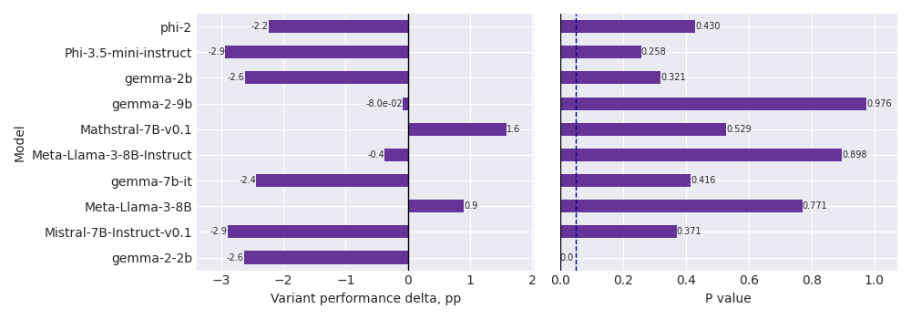
Model	GSM-Base acc	GSM-Variants acc	$\Delta$ Acc	P value	P value (Holm-Bonferroni)
phi-2	66.0	63.8	-2.24	0.430	1.000
Phi-3.5-mini-instruct	83.0	80.1	-2.94	0.258	1.000
gemma-2b	16.0	13.4	-2.62	0.321	1.000
gemma-2-9b	68.0	67.9	-0.08	0.976	1.000
Mathstral-7B-v0.1	78.0	79.6	1.58	0.529	1.000
Meta-Llama-3-8B-Instruct	75.0	74.6	-0.38	0.898	1.000
gemma-7b-it	43.0	40.6	-2.44	0.416	1.000
Meta-Llama-3-8B	49.0	49.9	0.90	0.771	1.000
Mistral-7B-Instruct-v0.1	47.0	44.1	-2.90	0.371	1.000
gemma-2-2b	25.0	22.4	-2.64	$\bm{<\delta}$	$\bm{<\delta}$

Table 12: Variant effect testing results obtained with the structured code prompt, as returned by GLMM 1. $\delta=0.001$. P values falling below the standard significance threshold $\alpha=0.05$ marked in bold.

Model	Odds ratio	95% CI	Z value	Std. error
phi-2	0.76	[0.39, 1.49]	-0.79	0.34
Phi-3.5-mini-instruct	0.63	[0.29, 1.40]	-1.13	0.40
gemma-2b	0.70	[0.34, 1.42]	-0.99	0.36
gemma-2-9b	0.99	[0.49, 2.01]	-0.03	0.36
Mathstral-7B-v0.1	1.28	[0.59, 2.80]	0.63	0.40
Meta-Llama-3-8B-Instruct	0.96	[0.50, 1.83]	-0.13	0.33
gemma-7b-it	0.77	[0.41, 1.45]	-0.81	0.32
Meta-Llama-3-8B	1.10	[0.59, 2.03]	0.29	0.31
Mistral-7B-Instruct-v0.1	0.77	[0.43, 1.38]	-0.89	0.30
gemma-2-2b	0.75	[0.75, 0.75]	-673.66	< 0.01

Table 13: Additional statistics for the variant effect testing with the structured code prompt, as returned by GLMM 1.

D.3 Additional Information on the Degenerate gemma-2-2b Fit

As mentioned in Sections 4.1 and 4.2, GLMM 1 results on gemma-2-2b are degenerate on the GSM prompt, structured NL prompt, and structured code prompt. Our further analysis shows that the coefficient estimates for gemma-2-2b are consistent and stable across all optimizers available in lme4 and all prompt formats (variant coefficient ranging from -0.24 to -0.45 log-odds across formats), as shown by the following results report:

Listing 6: Comparison of coefficient estimates for gemma-2-2b across optimisers.

⬇

1GSM prompt

2 (Intercept) is_variant

3bobyqa -2.358318 -0.3157934

4Nelder_Mead -2.358322 -0.3157909

5nlminbwrap -2.358319 -0.3157938

6nloptwrap.NLOPT_LN_NELDERMEAD -2.358201 -0.3158539

7nloptwrap.NLOPT_LN_BOBYQA -2.405811 -0.3077173

8

9====================

10

11Simple NL prompt

12 (Intercept) is_variant

13bobyqa -2.968160 -0.2415366

14Nelder_Mead -2.968176 -0.2415160

15nlminbwrap -2.968165 -0.2415333

16nloptwrap.NLOPT_LN_NELDERMEAD -2.968158 -0.2413823

17nloptwrap.NLOPT_LN_BOBYQA -2.968152 -0.2415481

18

19====================

20

21Structured NL prompt

22 (Intercept) is_variant

23bobyqa -2.006092 -0.4461784

24Nelder_Mead -2.006096 -0.4461799

25nlminbwrap -2.006091 -0.4461776

26nloptwrap.NLOPT_LN_NELDERMEAD -2.062258 -0.4470053

27nloptwrap.NLOPT_LN_BOBYQA -2.044976 -0.4464479

28

29====================

30

31Simple code prompt

32 (Intercept) is_variant

33bobyqa -2.252103 -0.2725128

34Nelder_Mead -2.252106 -0.2725081

35nlminbwrap -2.252113 -0.2725396

36nloptwrap.NLOPT_LN_NELDERMEAD -2.251930 -0.2726682

37nloptwrap.NLOPT_LN_BOBYQA -2.252078 -0.2725294

38

39====================

40

41Structured code prompt

42 (Intercept) is_variant

43bobyqa -2.383680 -0.2927124

44Nelder_Mead -2.469397 -0.2791749

45nlminbwrap -2.383678 -0.2927097

46nloptwrap.NLOPT_LN_NELDERMEAD -2.423186 -0.2933606

47nloptwrap.NLOPT_LN_BOBYQA -2.438184 -0.2782190

The estimates are unreliable for the three formats likely due to Hessian issues, not due to optimizer failure or identifiability problems. However, the underlying effect size is real and consistent; it is only the inferential statistics that should be deemed unreliable.

We acknowledge that alternative estimation frameworks—such as Bayesian GLMMs employing weakly informative priors or frequentist approaches utilizing Firth’s penalized likelihood—could theoretically regularize the fit and yield bounded uncertainty estimates for this degenerate case. However, applying a fundamentally different statistical regularization framework to rescue a single model’s estimates would introduce methodological inconsistency into our benchmark reproduction. Therefore, to maintain a rigorously uniform frequentist evaluation standard across all evaluated LLMs, we conservatively elect to report the degenerate fit and exclude gemma-2-2b from our primary inferential analyses.

D.4 The Large Number Effect

Figure 7 visualises the difference in distribution of integers occurring in questions from the GSM-Base and GSM-Variants datasets. In the latter, the distribution is shifted towards larger numbers with K-S statistic of 12 percentage points and high statistical significance ($p<0.001$), as reported in Section 3.4.

Figure 7: Distribution of integers extracted from problem texts in GSM-Base and GSM-Variants datasets. Top: counts of integers grouped into variable-width bins, normalised by the total of integers extracted from each dataset’s questions. Bottom: normalised cumulative counts of extracted numbers, zoomed for clearer presentation of the distribution shift.

Tables 14 and 15 present the results of the large number effect significance testing.

Model / prompt	GSM	simple NL	structured NL	simple code	structured code
phi-2	0.76 $\bm{<\delta}$ / $\bm{<\delta}$	0.71 $\bm{<\delta}$ / $\bm{<\delta}$	0.66 $\bm{<\delta}$ / $\bm{<\delta}$	0.90 0.277 / 0.554	1.00 0.972 / 0.972
Phi-3.5-mini-instruct	0.74 $\bm{<\delta}$ / $\bm{<\delta}$	0.77 $\bm{<\delta}$ / 0.002	0.80 $\bm{<\delta}$ / $\bm{<\delta}$	1.03 0.714 / 0.714	0.87 0.171 / 0.343
gemma-2b	0.84 0.040 / 0.121	0.80 0.011 / 0.046	0.78 0.003 / 0.013	0.98 0.747 / 1.000	0.97 0.716 / 1.000
gemma-2-9b	1.04 0.570 / 0.816	0.74 $\bm{<\delta}$ / 0.002	0.91 0.247 / 0.740	1.15 0.083 / 0.333	0.93 0.408 / 0.816
Mathstral-7B-v0.1	0.90 0.103 / 0.310	0.80 0.002 / 0.010	0.82 0.004 / 0.016	0.88 0.176 / 0.352	0.94 0.527 / 0.527
Meta-Llama-3-8B-Instruct	0.87 0.057 / 0.229	0.91 0.159 / 0.478	0.71 $\bm{<\delta}$ / $\bm{<\delta}$	1.01 0.866 / 0.866	1.07 0.373 / 0.746
gemma-7b-it	0.88 0.042 / 0.169	0.87 0.130 / 0.169	0.84 $\bm{<\delta}$ / $\bm{<\delta}$	0.85 0.055 / 0.169	0.86 0.082 / 0.169
Meta-Llama-3-8B	1.10 0.202 / 0.606	0.79 0.020 / 0.099	1.06 0.538 / 1.000	1.13 0.121 / 0.484	0.96 0.627 / 1.000
Mistral-7B-Instruct-v0.1	0.77 $\bm{<\delta}$ / $\bm{<\delta}$	0.84 $\bm{<\delta}$ / $\bm{<\delta}$	0.79 $\bm{<\delta}$ / 0.003	1.03 0.655 / 1.000	1.04 0.625 / 1.000
gemma-2-2b	0.82 $\bm{<\delta}$ / $\bm{<\delta}$	0.81 0.015 / 0.046	0.91 0.203 / 0.379	0.91 0.190 / 0.379	0.98 $\bm{<\delta}$ / $\bm{<\delta}$

Table 14: Odds ratios and significance of the large number effect across models and prompt formats, as returned by GLMM 2. Cells formatted as: (top row) odds ratio; (bottom row) raw P value / Holm-Bonferroni-corrected (column-wise) P value. $\delta=0.001$. P values falling below the standard significance threshold $\alpha=0.05$ marked in bold.

prompt	GSM	simple NL	structured NL	simple code	structured code
model
phi-2	0.31 $\bm{<\delta}$ / $\bm{<\delta}$	0.67 0.211 / 0.423	0.35 $\bm{<\delta}$ / 0.003	1.72 0.125 / 0.376	0.76 0.433 / 0.433
Phi-3.5-mini-instruct	0.59 0.220 / 0.660	1.41 0.346 / 0.693	1.17 $\bm{<\delta}$ / $\bm{<\delta}$	0.49 0.085 / 0.340	0.74 0.480 / 0.693
gemma-2b	0.48 0.038 / 0.153	0.33 0.002 / 0.008	2.05 0.091 / 0.273	0.96 0.910 / 0.910	0.72 0.389 / 0.777
gemma-2-9b	0.40 0.009 / 0.047	0.72 0.369 / 1.000	1.02 0.958 / 1.000	0.65 0.228 / 0.911	1.00 0.990 / 1.000
Mathstral-7B-v0.1	0.49 0.051 / 0.254	0.85 0.629 / 1.000	1.28 0.472 / 1.000	1.90 0.103 / 0.413	1.24 0.619 / 1.000
Meta-Llama-3-8B-Instruct	0.60 0.131 / 0.596	0.82 0.512 / 1.000	0.74 0.372 / 1.000	0.60 0.119 / 0.596	0.80 0.536 / 1.000
gemma-7b-it	0.58 0.060 / 0.238	1.27 0.525 / 1.000	1.12 $\bm{<\delta}$ / $\bm{<\delta}$	0.60 0.127 / 0.382	0.91 0.767 / 1.000
Meta-Llama-3-8B	0.45 0.011 / 0.056	0.65 0.254 / 0.698	0.63 0.233 / 0.698	1.75 0.071 / 0.285	1.14 0.699 / 0.699
Mistral-7B-Instruct-v0.1	0.67 0.151 / 0.606	1.14 $\bm{<\delta}$ / $\bm{<\delta}$	0.79 0.434 / 0.949	1.19 0.576 / 0.949	0.73 0.316 / 0.949
gemma-2-2b	0.91 $\bm{<\delta}$ / $\bm{<\delta}$	0.99 0.986 / 1.000	0.71 0.274 / 0.823	0.85 0.611 / 1.000	0.76 $\bm{<\delta}$ / $\bm{<\delta}$

Table 15: Odds ratios and significance of the large-number-effect-corrected variant effect across models and prompt formats, as returned by GLMM 2. Cells formatted as: (top row) odds ratio; (bottom row) raw P value / Holm-Bonferroni-corrected (column-wise) P value. $\delta=0.001$. P values falling below the standard significance threshold $\alpha=0.05$ marked in bold.

Figure 8 summarises the results of the large number effect test (see Sections 3.4 and 3.5).

Figure 8: Variant effect and large number effect - a combined case study of six LLMs. Top: log-odds ratio for variant effect (performance change on GSM-Variants vs GSM-Symbolic; $Variant$, GLMM 1). Middle: log-odds ratio for large number effect ($\gamma_{c}$, GLMM 2). Bottom: log-odds ratio for variant effect, corrected for the large number effect ($Variant$, GLMM 2). Hatching indicates the respective effect is not significant (p > 0.05, uncorrected).

Appendix E Failure Modes

In both natural-language and code prompt experiments, we predefine classes of errors and issues we anticipated to see when evaluating LLMs answers - in addition to miscalculation errors (where an incorrect numerical answer is returned; in the visualisations which follow, this is marked as Wrong answer). For natural language prompts, the classes are:

• Empty response - if the response is empty (zero-length);

• Empty (after trimming) - if the response only contains whitespaces and, optionally, the ’Q:’ token, indicating that the model is starting to generate a new question following the few-shot format;

• No number found - if all of our numerical answer extraction methods fails on a given answer;

• Wong answer - last number - if the incorrect numerical answer is also associated with the model not following the few-shot formatting guidelines, resulting in the answer being extracted through a simple regular expression capturing the last number in the text.

For code prompts, we define the following classes:

• No function - if a function definition can not be found in the model’s answer using a simple regular expression approach;

• Forbidden string - if the answer contains any string with potentially dangerous effects if executed, such as open(...) or eval(...);

• Syntax error - if executing the extracted function results in a SyntaxError;

• Name error - if a NameError is raised;

• Type/Value error - if a TypeError or ValueError is raised;

• Zero division error - if a ZeroDivisionError is raised;

• Attribute error - if an AttributeError is raised;

• None returned - if the function does not return any value, either by skipping a return line, using empty return, or returning None explicitly;

• Not a number - if the value returned from the function is not numerical and other than None;

• Unclassified - all remaining error cases encountered when running the extracted function.

E.1 Failure Modes in NL Prompts

Figure 9: Total counts of error types in the three NL prompts: the original GSM prompt (top), simple NL prompt (middle) and structured NL prompt (bottom).

As shown in Figure 9, incorrect numerical response constitutes the overwhelming majority of errors in NL prompts experiments. There is also a considerable portion of the last-number numerical results (in total: 9% in the GSM prompt; 4% in the simple NL prompt; 5% in the structured NL prompt). The failed formatting cases varies in the underlying patterns. In some cases, the models indeed simply “forget” to introduce the answer with the required line (The final answer is…). In other cases, as shown below, the lack of adherence to formatting is a result of a cognitive failure, with the model getting lost in a potentially infinite loop of operations, often resulting in unreasonably high numerical answers.

Listing 7: phi-2’s answer to question: “Liam hires a luxury car from 3 PM to 9 PM. He gets 1 hours free. The first paid hour is $13 and each hour after that is twice the cost. How much did he pay?”.

⬇

1The first paid hour is $13. The second paid hour is $13 * 2 = $26. The third paid hour is $26 * 2 = $52. The fourth paid hour is $52 * 2 = $104. The fifth paid hour is $104 * 2 = $208. The sixth paid hour is $208 * 2 = $416. The seventh paid hour is $416 * 2 = $832. The eighth paid hour is $832 * 2 = $1664. The ninth paid hour is $1664 * 2 = $3328. The tenth paid hour is $3328 * 2 = $6656. The eleventh paid hour is $6656 * 2 = $13112. The twelfth paid hour is $13112 * 2 = $26224. The thirteenth paid hour is $26224 * 2 = $52448. The fourteenth paid hour is $52448 * 2 = $104896. The fifteenth paid hour is $104896 * 2 = $2087328. The sixteenth paid hour is $2087328 * 2 = $41657656. The seventeenth paid hour is $41657656 * 2 = $81315352. The eighteenth paid hour is $81315352 * 2 = $162630704. The nineteenth paid hour is $162630704 * 2 = $325266048. The twentieth paid hour is $325266048 * 2 = $650532096. The twenty-first paid hour is $650532096 * 2 = $1301056096. The twenty-second paid hour is $1301056096 * 2 = $26011092192. The twenty-third paid hour is $26011092192 * 2 = $5220184384. The twenty-fourth paid hour is $5220184384 * 2 = $10440368768. The twenty-fifth paid hour is $10440368768 * 2 = $208807375536. The twenty-sixth paid hour is $208807375536 * 2 = $416165750272. The twenty-seventh paid hour is $416165750272 * 2 = $8321715010544. The twenty-eighth paid hour is $8321715010544 * 2 = $16653430209888. The twenty-ninth paid hour is $16653430209888 * 2 = $331327604019616. The thirtieth paid hour is $331327604019616 * 2 = $662655208039328. The thirty-first paid hour is $662655208039328 * 2 = $1325322108079264. The thirty-second paid hour is $1325322108079264 * 2 = $26506452080392816. The thirty-third paid hour is $26506452080392816 * 2 = $51230105207926352. The thirty-fourth paid hour is $51230105207926352 * 2 = $102460110407953504. The thirty-fifth paid hour is $102460110407953504 * 2 = $2049242080791050984. The thirty-sixth paid hour is $2049242080791050984 * 2 = $4098484080792099008. The thirty-seventh paid hour is $4098484080792099008 * 2 = $819699680792099016. The thirty-eighth paid hour is $819699680792099016 * 2 = $1639739960792099032. The thirty-ninth paid hour is $1639739960792099032 * 2 = $3238799207920990528. The fortieth paid hour is $3238799207920990528 * 2 = $657599407920991056. The forty-first paid hour is $657599407920991056 * 2 = $1315099879209920112. The forty-second paid hour is $1315099879209920112 * 2 = $2630199587920992424. The forty-third paid hour is $2630199587920992424 * 2 = $5230199167920994848. The forty-fourth paid hour is $5230199167920994848 * 2 = $1050699335879209996. The forty-fifth paid hour is $1050699335879209996 * 2 = $2010399667920999824. The forty-sixth paid hour is $20103996679209998

Yet another pattern worth noting is the models’ calculations leading to an implausible result, with the models acknowledging the character of the result, as shown below.

Listing 8: Meta-Llama-3-8B-Instruct’s answer to question: “At the beginning of the conference, there were 29 engineers and 15 artists. After an hour, one-fourth of the total number of people left. How many artists are left if 27 engineers stayed at the conference?”.

⬇

1Given:

2Number of engineers originally: 29

3Number of artists originally: 15

4Number of engineers who stayed: 27

5

6To find: number of artists left.

7

8Solution:

9First, calculate the total number of people originally:

1029 + 15 = 44

11Next, calculate the number of people who left:

121/4 * 44 = 11

13Next, calculate the number of artists who left:

1411 - 27 = 16

15Finally, calculate the number of artists left:

1615 - 16 = -1 (which is impossible, so there must be an error in the question)

17

18The final answer is unknown due to the error in the question.

In some cases, as shown below, the models in fact follow the reply formatting guidelines as closely as possible despite the lack of satisfactory numerical answers.

Listing 9: Mistral-7B Instruct-v0.1’s answer to question: “When Valeria watches her nephew, she gets out a variety of toys for him. The bag of building blocks has 71 blocks in it. The bin of stuffed animals has 47 stuffed animals inside. The tower of stacking rings has 30 multicolored rings on it. Valeria recently bought a tube of bouncy balls, bringing her total number of toys for her nephew up to 238. How many bouncy balls came in the tube?”.

⬇

171 blocks + 47 stuffed animals + 30 multicolored rings = 158. Valeria has 238 toys in total. 158 - 238 = -80. This is not possible. The final answer is that there is an error in the problem statement.

Among cases of empty answers, Meta-Llama-3-8B presents an interesting case, with disproportionally high numbers of such failures in the simple and structured prompts, and higher counts associated with the more complex prompt format. Moreover, phi-2 fails to provide any answer to a considerable number of questions, but only in the canonical, GSM prompt format.

E.2 Failure Modes in Code Prompts

Figure 10: Total per-model error counts on the GSM-Variants dataset for the two code prompts: simple code prompt (top) and structured code prompt (bottom).

Figure 11: Proportions of per-model errors other than wrong answer on the GSM-Variants dataset, for the two code prompts: simple code prompt (top) and structured code prompt (bottom).

Similarly to NL prompts, mistakes in code prompts are predominantly of numerical nature - as shown in Figure 10. Among other error types (see Figure 11), we observe 7 of the predefined 10 classes, with name, syntax, and none-returned errors constituting the majority for both prompt formats. We encounter only two cases in which errors are out of the scope of our predefined categories. One of them is an overflow error due to the model falling into a loop of generating the same digit (0) without a space (see Listing 10 below). The other is a key error caused by the model (Mistral-7B-Instruct-v0.1) attempting to access a non-existing item in a previously defined dictionary.

Listing 10: gemma-2b’s response on a simple code prompt task, triggering an overflow error.

⬇

1 apartments_before = 5

2 apartments_per_complex = 350

3 apartments_per_complex_total = apartments_before * apartments_per_complex

4 apartments_per_complex_total_75 = apartments_per_complex_total * 0.75

5 apartments_per_complex_total_sum = apartments_per_complex_total + apartments_per_complex_total_75

6 apartments_per_complex_total_sum_3 = apartments_per_complex_total_sum * 3

7 apartments_per_complex_total_sum_3_pay = apartments_per_complex_total_sum_3 * 0.5

8 apartments_per_complex_total_sum_3_pay_total = apartments_per_complex_total_sum_3_pay * apartments_per_complex_total_sum_3

9 apartments_per_complex_total_sum_3_pay_total_sum = apartments_per_complex_total_sum_3_pay_total + 100000000000000000000000000000000000000000000000000000000000000000000000000000000000000000000000000000000000000000000 000000000000000000000000000000000000000000000000000000000000000000000000000000000000000000000000000000000000000000000 000000000000000000000000000000000000000000000000000000000000000000000000000000000000000000000000000000000000000000000 000000000000000000000000000000000000000000000000000000000000000000000000000000000000000000000000000000000000000000000 000000000000000000000000000000000000000000000000000000000000000000000000000000000000000000000000000000000000000000000 000000000000000000000000000000000000000000000000000000000000000000000000000000000000000000000000000000000000000000000 0000000000000000000000000000000000000000000000000000000000000000000000000000000