

11email: {gunw0, chase121, jongwoo.lim}@snu.ac.kr
LC-Flow: Learning Local Continuous Optical Flow and Confidence from events
Abstract
Event cameras capture brightness changes asynchronously with microsecond resolution, yet existing optical flow methods fail to fully exploit this temporal continuity. Frame-based approaches impose artificial accumulation latency and suffer from domain overfitting, while model-based local methods operate statelessly, discarding temporal history between predictions and yielding inaccurate flows.
We propose LC-Flow, the first temporally continuous, learning-based optical flow estimator that operates purely from local events. At its core, a Continuous Local Recurrent Network maintains persistent hidden states per spatial grid, incrementally accumulating temporal context as events arrive. Unlike frame-based methods constrained to fixed accumulation windows, and unlike stateless model-based methods that recompute motion from scratch at each step, LC-Flow produces sparse local flow estimates at arbitrary timestamps with full motion history.
To address the inherent ambiguity of local observations, we jointly learn a confidence score that quantifies the reliability of each prediction, explicitly handling event sparsity and the aperture problem. This confidence serves a dual role: filtering unreliable estimates for downstream tasks such as visual odometry, and providing principled weights for a multi-scale confidence-guided aggregation that reconstructs globally consistent flow from the sparse local outputs. LC-Flow achieves state-of-the-art performance among local methods on both MVSEC and DSEC, while the confidence-guided aggregation establishes a new overall state-of-the-art on the MVSEC benchmark, surpassing heavy frame-based networks that rely on global spatial priors.
1 Introduction
Event cameras are bio-inspired sensors that asynchronously capture per-pixel brightness changes. With microsecond temporal resolution and high dynamic range, they are inherently suited for high-speed motion estimation in challenging environments. To fully exploit these advantages in real-world applications such as visual odometry (VO) and target tracking, motion estimation systems ideally process events incrementally and locally, preserving the sensor’s continuous-time nature instead of imposing fixed, dense frames that quantize time. However, accurate optical flow estimation from purely asynchronous, local observations remains challenging. Existing methods largely fall into two polarized paradigms: dense learning-based approaches and sparse local approaches.
Dense methods [eraft, liu2025edcflow] achieve remarkable accuracy by accumulating sparse events into synchronous representations (e.g., voxel grids) to leverage powerful deep neural networks. However, this paradigm introduces inevitable accumulation latency and is highly prone to domain overfitting due to its reliance on global spatial priors. Conversely, local and incremental methods [akolkar2020real, nagata2023tangentially, yuan2024learning] respect the asynchronous nature of events by estimating motion directly from localized patches. Yet, because they operate statelessly without retaining temporal history, they remain limited by simplified geometric assumptions or handcrafted priors, inherently suffering from the aperture problem and sensitivity to noise in complex real-world scenes.
To bridge this gap, we propose LC-Flow, the first temporally continuous, learning-based optical flow framework that extracts full 2D motion and confidence purely from local event dynamics. Unlike frame-based networks, we avoid global context aggregation to prevent domain overfitting. Instead, we introduce a Continuous Local Recurrent Network that assigns an independent, persistent hidden state to each local grid. Rather than slicing time into discrete, memoryless windows, the hidden states are updated incrementally as every event arrives. This enables truly continuous inference: flow can be queried at any arbitrary timestamp with full motion history, a capability that neither frame-based recurrent methods nor stateless model-based approaches can provide.
The core output of LC-Flow is a sparse local flow field, which is the primary contribution of this work. This sparse representation is directly usable for downstream tasks such as VO and tracking, where reliable motion cues at active pixel locations are sufficient. However, relying solely on highly localized patches inevitably encounters the aperture problem, where motion along uniform edges remains ambiguous. To explicitly handle this, we jointly learn a confidence score that quantifies the reliability of each grid’s flow prediction based on its local spatiotemporal evidence.
We demonstrate that our localized estimations are not limited to sparse outputs. By applying a multi-scale confidence-guided aggregation, we propagate highly reliable motion cues to uncertain regions, seamlessly reconstructing a globally consistent flow field without global feature aggregation. Evaluated on the standard MVSEC benchmark, this extension achieves state-of-the-art performance, surpassing heavy frame-based dense networks that rely on global spatial priors. This demonstrates that high-quality local dynamics, coupled with explicit uncertainty estimation, are sufficient to overcome the domain overfitting issues of global architectures.
Our main contributions are summarized as follows:
-
1.
Temporally Continuous Local Architecture: We propose the first temporally continuous, learning-based local recurrent network for event-based optical flow estimation. By maintaining persistent hidden states that are updated with every incoming event, our method enables temporally coherent flow estimation at arbitrary timestamps. Unlike stateless model-based methods that recompute motion without retaining temporal history, and frame-based methods that are constrained to fixed accumulation boundaries, our architecture continuously accumulates motion history while remaining asynchronous.
-
2.
Uncertainty-Aware Confidence Learning: We introduce a joint flow and confidence learning mechanism that quantifies the reliability of local predictions, explicitly addressing event sparsity and the aperture problem. The learned confidence serves a dual role: filtering unreliable estimates for downstream applications and providing principled weights for global flow reconstruction.
-
3.
State-of-the-Art Results: Our method establishes state-of-the-art for local event-based optical flow on both MVSEC and DSEC. Furthermore, we demonstrate that multi-scale confidence-guided aggregation of these local outputs achieves overall state-of-the-art on the MVSEC benchmark, outperforming dense frame-based baselines.
2 Related Works
2.1 Dense Optical Flow Estimation from Event Cameras
Dense optical flow estimation from event cameras has attracted increasing attention, yet remains challenging because event streams are sparse, asynchronous, and noisy.
Model-based approaches estimate motion by explicitly modeling event generation and optimizing geometric consistency. Multi-CM [shiba2022secrets] reconstructs sharp edge structures through contrast maximization, while other methods exploit handcrafted spatio-temporal surfaces such as time-surfaces or distance-surfaces for matching-based motion inference [nagata2021optical, almatrafi2020distance]. These approaches are often computationally efficient, but brittle in complex scenes.
Learning-based dense methods typically bridge asynchrony by accumulating events into synchronous, frame-like representations to leverage high-capacity CNNs. EV-FlowNet [zhu2018ev] uses event-count representations with photometric consistency losses, while E-RAFT [eraft], TMA [liu2023tma], and EDCFlow [liu2025edcflow] adapt modern image-flow architectures to voxel grid inputs. While these methods achieve excellent benchmark accuracy, fixed-window voxelization introduces unavoidable accumulation latency and makes performance sensitive to inference frequency. Moreover, reliance on globally aggregated features can increase sensitivity to scene domain shifts.
A parallel line explores SNN-based models for low-latency dense inference [lee2020spike, cuadrado2023optical, zhang2023event], although stabilizing training and achieving competitive accuracy remain challenging.
2.2 Local and Incremental Flow Estimation
Beyond dense flow, several works estimate local sparse motion directly from event streams to exploit microsecond temporal resolution and achieve low-latency inference. Classical techniques, such as Lucas–Kanade (LK)-based methods [barranco2014contour], compute motion from localized spatio-temporal neighborhoods but inevitably suffer from the aperture problem.
A number of methods aim to improve robustness and mitigate the aperture problem within this sparse local paradigm. ARMSflow [akolkar2020real] employs robust kinematic plane fitting, VecKMFlow [Veckmflow] predicts normal flow from compact event patches, and Shiba et al. [shiba2023fast] propose event-by-event triplet matching to align events across space and time. To share information across spatial neighborhoods, TEGBP [nagata2023tangentially] propagates tangentially elongated Gaussians via belief propagation; however, such approaches typically rely on explicit smoothness assumptions and handcrafted noise models, which can become brittle in complex real-world scenes. More broadly, these local methods do not maintain a learned persistent memory that is updated continuously with incoming events, limiting their ability to accumulate temporal context over time. To our knowledge, LC-Flow is the first local learning-based method to maintain persistent hidden states per local grid, enabling continuous inference with accumulated temporal context.
Beyond benchmarking, local sparse flow is also valuable for downstream tasks such as visual odometry and target tracking, where reliable motion cues at active locations facilitate data association [wang2023lightweight, senst2012robust, liu2022robust, zeng2021robust]. This further motivates estimating prediction confidence for reliable deployment.
2.3 Continuous-Time and Streaming Representations for Event Data
A growing body of work argues that the dominant windowed-to-dense paradigm introduces inherent latency and obscures fine-grained temporal structure, partially negating the advantages of event cameras. Several studies show that temporal binning and interpolation discard informative event ordering cues, motivating alternative representations that preserve temporal continuity [baldwin2021tore, lin2024ces]. Recent analyses further report that models trained under a fixed accumulation rate may generalize poorly when deployed at different inference frequencies [zubic2024ssm, flexevent2024].
These concerns have also driven interest in streaming and continuous-time processing across event-based vision. One line of work performs sparse, event-by-event computation via recurrent updates or sparse message passing [sekikawa2019eventnet, schaefer2022aegnn]. Another develops state-space formulations that maintain persistent latent states and update them incrementally over time [zubic2024ssm, kappel2024dssm]. Complementary ideas appear in continuous-time motion modeling, where the output is represented as a continuous-time field to reduce aliasing from discrete-time predictions [wang2025continuousmotionfield].
Together, these trends motivate our design choice: rather than repeatedly aggregating events into dense windows, we maintain persistent local hidden states and update them online. This enables computation that adapts to local scene activity, preserves temporal continuity, and avoids the latency and brittleness introduced by fixed-window accumulation.

3 Method
As illustrated in Fig. 1, LC-Flow consists of two components: (i) a Continuous Local Recurrent Network that estimates flow and confidence purely from local events while maintaining a persistent hidden state for each local grid , enabling event-driven flow querying at arbitrary timestamps from the per-grid event stream , and (ii) a Confidence-guided Aggregator that reconstructs a global flow field from these sparse local predictions.
3.1 Continuous Local Recurrent Network
3.1.1 Problem Formulation.
Given a continuous stream of asynchronous events , our goal is to estimate, at any timestamp , the optical flow and a confidence score at pixel . We define as the displacement over a short interval , where is set to match the dataset’s ground-truth annotation interval for convenience. Instead of waiting for a fixed accumulation window, LC-Flow updates the estimates incrementally as events arrive by continuously integrating motion history into the network’s hidden state.
3.1.2 Event Embedding.
Each event is represented by its spatial location, timestamp, and polarity, . We process events locally within a neighborhood centered at grid location , where is an odd integer. Spatial coordinates are normalized relative to the grid center, and temporal information is encoded using the inter-event interval. The local event embedding is defined as
| (1) |
where scales the temporal component (we set in practice so that typical inter-event intervals have a magnitude comparable to the normalized spatial terms). We initialize to the timestamp of the first event in each grid. This embedding maps local spatial coordinates to and captures relative temporal dynamics rather than absolute time.
3.1.3 Continuous GRU Update.
We utilize a Gated Recurrent Unit (GRU) [chung2014gru] to aggregate temporal information by maintaining a persistent hidden state per grid:
| (2) |
The hidden state is updated for every incoming event, accumulating motion context over arbitrary durations without imposing fixed temporal boundaries. We adopt GRU for its simplicity and training stability, which we find well suited to lightweight per-event updates.
3.1.4 Prediction Heads.
The hidden state is fed into two separate MLP heads. The flow head outputs a 2D flow vector at the grid center , denoted . The confidence head outputs a scalar via a sigmoid activation, representing the estimated reliability of given the local spatiotemporal evidence.
3.1.5 Loss.
We jointly optimize the flow and confidence heads using a confidence-weighted regression objective inspired by uncertainty-based weighting [kendall2017uncertainties]:
| (3) |
where and denote the predicted and ground-truth flow at the supervised location, is the predicted confidence, and is a balancing coefficient. The first term penalizes the flow error weighted by confidence, while the second term regularizes to prevent the trivial solution of driving confidence toward zero.
3.2 Confidence-guided Aggregator
While our local estimator outputs accurate sparse flow and confidence at selected grid centers, some applications require a global flow field. We therefore reconstruct a global flow map via a lightweight, patch-based aggregation module that propagates reliable local motion to nearby uncertain or inactive regions.
3.2.1 Grid-wise Recurrent Processing with Spatial Striding.
We deploy the local estimator only at grid centers sampled with stride . Each deployed grid maintains an independent recurrent hidden state updated solely by events within its spatial neighborhood, and there is no interaction across grids. Striding provides a direct trade-off between spatial coverage and computation, and empty grids (with insufficient events) are skipped.
3.2.2 Multi-scale Confidence-guided Aggregation.
At each deployed grid center, LC-Flow predicts a local flow vector and confidence. For a given scale (corresponding to a specific stride), we first bilinearly interpolate the sparse predictions to obtain an intermediate flow map and confidence map at full resolution. We then compute a confidence-weighted local average over a neighborhood for each target pixel :
| (4) |
where is a small constant for numerical stability.
To fuse information across scales without uniformly averaging, we adaptively predict per-scale fusion weights from the local multi-scale evidence. Specifically, we stack the flow (2 channels) and confidence (1 channel) from each scale within the neighborhood into a local tensor . A lightweight patch-based CNN then predicts soft fusion weights:
| (5) |
The final aggregated flow is
| (6) |
3.3 Training Strategy
3.3.1 Training Data Construction.
We construct training samples from temporally sliced event streams provided by standard event-based optical flow benchmarks. Each slice is partitioned into local grids of size . A grid is considered valid if it contains at least 10 events, ensuring sufficient local motion evidence. For each valid grid, we extract the corresponding per-grid event sequence and supervise the flow at the grid center using the slice-level ground-truth. This grid-wise construction yields a large set of local event streams paired with flow supervision and mirrors our inference-time processing.
3.3.2 Continuous Training Strategy.
Training on a single slice provides short-term supervision but does not expose the recurrent state to the long temporal evolution required for streaming inference. To simulate continuous deployment, we form a training sample by concatenating consecutive slices, where is uniformly sampled from a fixed range. The model processes all slices sequentially to update the hidden state, while flow supervision is applied only at the final slice. This forces the network to maintain stable temporal representations over varying durations and aligns training with event-driven inference at test time.
3.3.3 Data Augmentation.
To improve generalization and robustness to local motion variations, we apply augmentation directly to the extracted local event streams. Geometric transforms are applied consistently to both event coordinates and ground-truth flow vectors:
-
•
Reflection. Reflect events horizontally or vertically about the grid center, and transform flow accordingly.
-
•
Rotation. Rotate events around the grid center. We use both right-angle rotations (, , ) and random rotations sampled uniformly from . For arbitrary angles, rotated coordinates are rounded to the nearest pixel to preserve the discrete grid structure.
-
•
Polarity Reversal. Invert event polarities to simulate contrast changes, leaving spatial and temporal coordinates unchanged.
4 Experiments
4.1 Experimental Setup
Datasets. We evaluate our method on MVSEC [zhu2018mvsec] and DSEC [gehrig2021dsec]. For MVSEC, the local flow model is trained exclusively on the outdoor_day2 sequence and evaluated on outdoor_day1 and indoor_flying1,2,3, following the standard evaluation protocol. For DSEC, all official training sequences excluding zurich_city_02a are used for training, and zurich_city_02a is held out for evaluation.
Local Flow Model Configuration. For MVSEC, the image space is partitioned into local grids of size pixels, and each grid maintains an independent GRU with a hidden dimension of 256. The network is trained using the Adam optimizer with a batch size of 512 and a learning rate of . For DSEC, to accommodate the higher spatial resolution, we use a grid size of pixels, a hidden dimension of 256, a batch size of 256, and a learning rate of .
Training Schedule. The GRU, flow, and confidence heads are jointly trained for 450K iterations on MVSEC and 388K iterations on DSEC, with the confidence balancing coefficient set to and , respectively. Each training sample is constructed by concatenating consecutive temporal slices, where is uniformly sampled from for both datasets.
Data Augmentation. We apply the grid-level augmentations described in Sec.˜3.3 with the following probabilities. Discrete right-angle rotations of and are independently applied with a 25% probability each. Additionally, one of three supplementary augmentations is randomly applied with a ratio of : event polarity reversal, spatial reflection (randomly chosen along the - or -axis), and random rotation with angles uniformly sampled from .
Confidence-guided Aggregator. We deploy the local model with stride and perform multi-scale aggregation with patch size and scales on MVSEC. The local model weights are frozen during aggregator training. The aggregator is trained on the same sequences as the local model for 50 epochs with a learning rate of .
| Method | Type | MVSEC | DSEC | ||||||||||||
| Outdoor1 | Indoor1 | Indoor2 | Indoor3 | Zurich 02a | |||||||||||
| PEE | EPE | %out | PEE | EPE | %out | PEE | EPE | %out | PEE | EPE | %out | EPE | %out | ||
| Inference on MVSEC image frequency | |||||||||||||||
| Triplet [shiba2023fast] | MB | - | 0.90 | 3.1 | - | 1.10 | 2.9 | - | 1.70 | 13.4 | - | - | - | - | - |
| VecKM [Veckmflow] | SL | 0.88 | - | - | 0.97 | - | - | 1.09 | - | - | 1.04 | - | - | - | - |
| ARMS [akolkar2020real] | MB | - | 2.75 | - | - | 1.52 | - | - | 1.59 | - | - | 1.89 | - | 8.98 | 78.7 |
| Ours | SL | 0.19 | 0.24 | 0.05 | 0.32 | 0.48 | 0.20 | 0.40 | 0.62 | 0.58 | 0.37 | 0.58 | 0.49 | - | - |
| Inference on s | |||||||||||||||
| TEGBP [nagata2023tangentially] | MB | - | 1.46 | 11.1 | - | 1.14 | 6.25 | - | 1.87 | 16.4 | - | 1.54 | 11.8 | 8.70 | 72.6 |
| Ours | SL | - | 0.93 | 1.76 | - | 0.98 | 1.46 | - | 1.56 | 8.03 | - | 1.43 | 7.30 | 2.10 | 17.3 |
4.2 Evaluation Metrics
We report three metrics. Endpoint Error (EPE) is the mean Euclidean distance between predicted and ground-truth flow over all valid pixels. Outlier Ratio (%Out) is the percentage of valid pixels with EPE larger than 3 pixels. Projected Endpoint Error (PEE) follows the normal-flow evaluation of VecKMFlow [Veckmflow], computing EPE after projecting the ground-truth flow onto the direction of the predicted flow.
| Method | Outdoor1 | Indoor1 | Indoor2 | Indoor3 | Avg. | Avg. | |||||
| EPE | Out | ||||||||||
| () | EPE | % Out | EPE | % Out | EPE | % Out | EPE | % Out | |||
| MB | Brebion et al. [brebion2021real] | 0.53 | 0.20 | 0.52 | 0.10 | 0.98 | 5.50 | 0.71 | 2.10 | 0.69 | 1.98 |
| Nagata et al. [nagata2021optical] | 0.77 | - | 0.62 | - | 0.93 | - | 0.84 | - | 0.79 | - | |
| MultiCM [shiba2022secrets] | 0.30 | 0.10 | 0.42 | 0.10 | 0.60 | 0.59 | 0.50 | 0.28 | 0.46 | 0.27 | |
| USL | FireFlowNet [paredes2021back] | 1.06 | 6.60 | 0.97 | 2.60 | 1.67 | 15.30 | 1.43 | 11.00 | 1.28 | 8.88 |
| EV-MGRFlow [zhuang2024ev] | 0.28 | 0.02 | 0.41 | 0.17 | 0.70 | 2.35 | 0.59 | 1.29 | 0.50 | 0.96 | |
| Zhu et al. [zhu2019unsupervised] | 0.32 | 0.00 | 0.58 | 0.00 | 1.02 | 4.00 | 0.87 | 3.00 | 0.70 | 1.75 | |
| SSL | EV-FlowNet [zhu2018ev] | 0.49 | 0.20 | 1.03 | 2.20 | 1.72 | 15.10 | 1.53 | 11.90 | 1.19 | 7.35 |
| STE-FlowNet [ding2022spatio] | 0.42 | 0.00 | 0.57 | 0.10 | 0.79 | 1.60 | 0.72 | 1.30 | 0.63 | 0.75 | |
| SL | Matrix-LSTM [cannici2020differentiable] | - | - | 0.82 | 0.53 | 1.19 | 5.59 | 1.08 | 4.81 | 1.03 | 3.64 |
| E-RAFT [eraft] | 0.24 | 0.00 | 1.10 | 5.72 | 1.94 | 30.79 | 1.66 | 25.20 | 1.24 | 15.43 | |
| DCEIFlow [wan2022learning] | 0.22 | 0.00 | 0.75 | 1.55 | 0.90 | 2.10 | 0.80 | 1.77 | 0.67 | 1.36 | |
| EDCFlow [liu2025edcflow] | 0.23 | 0.00 | 0.97 | 2.19 | 1.49 | 10.79 | 1.38 | 8.98 | 1.02 | 5.49 | |
| TMA [liu2023tma] | 0.25 | 0.07 | 1.06 | 3.63 | 1.81 | 27.29 | 1.58 | 23.26 | 1.18 | 13.56 | |
| Ours | 0.21 | 0.04 | 0.40 | 0.00 | 0.55 | 0.30 | 0.50 | 0.14 | 0.42 | 0.14 | |


4.3 Results
Local flow estimation. We first evaluate the Continuous Local Recurrent Network against recent local and incremental methods (Tab.˜1). To measure intrinsic accuracy, we deploy the local estimator densely at all pixel locations, independent of the striding and aggregation used in the full pipeline. LC-Flow outperforms existing baselines across all MVSEC sequences, achieving an EPE of on Outdoor Day 1 and on Indoor Flying 3. Although our model is trained to predict full 2D flow (not normal flow), it attains lower PEE than VecKMFlow, which is designed specifically for normal-flow estimation. This suggests that accurate full-flow predictions capture normal-flow components as well. For a fair comparison with TEGBP at its reported evaluation interval, we additionally evaluate at , where LC-Flow also outperforms TEGBP across all sequences. On DSEC, LC-Flow substantially outperforms ARMSflow and TEGBP, achieving an EPE of compared to and , respectively.
Flow reconstruction via Confidence-guided Aggregation. Next, we compare our full pipeline against other optical flow networks (Tab.˜2). Our method establishes a new state-of-the-art, achieving the lowest average EPE of and an outlier ratio of . Notably, while heavy supervised methods such as E-RAFT and EDCFlow degrade significantly on indoor sequences (e.g., E-RAFT yields an EPE of on Indoor 2), our method achieves on the same sequence. Furthermore, even on Outdoor Day 1 where global methods hold a natural advantage, our confidence-guided aggregation achieves an EPE of , surpassing DCEIFlow () and EDCFlow (). Fig.˜2 presents qualitative comparisons on the MVSEC Indoor Flying 3 scene against EVFlowNet [zhu2018ev] (SSL), Multi-CM [shiba2022secrets] (MB), and DCEIFlow [wan2022learning] (SL). LC-Flow produces accurate flow predictions closely aligned with the ground truth, while competing methods exhibit noisy or incorrect estimates. Results on DSEC are included in the supplementary material.
| Training | Inference reset interval | ||||
|---|---|---|---|---|---|
| Every 1 | Every 2 | Every 4 | Every 8 | No reset | |
| Single slice () | 1.17 | 1.33 | 1.98 | 2.82 | 4.19 |
| Random slices () | 1.24 | 1.06 | 0.88 | 0.73 | 0.58 |
| Method | Inference Time | EPE |
|---|---|---|
| (ms/frame) | () | |
| Multi-CM [shiba2022secrets] | 8000 | 0.30 |
| E-RAFT [eraft] | 13.66 | 0.24 |
| VecKM-Flow [yuan2024learning] | 82.42 | |
| LC-Flow (Ours) | ||
| #0 Bilinear (s=3) | 13.00 | 0.23 |
| #4 Conf-guided Agg (s=3) | 31.81 | 0.21 |
| #3 Conf Avg (s=3) | 13.16 | 0.21 |
| #3 Conf Avg (s=4) | 8.71 | 0.21 |
| #3 Conf Avg (s=5) | 6.63 | 0.21 |
| † PEE; a lower bound of EPE. | ||
4.4 Effect of Confidence
To validate the learned confidence measure, we analyze the correlation between predicted confidence scores and actual estimation errors across MVSEC sequences. As shown in Fig.˜3, all error metrics decrease monotonically as the confidence threshold increases, consistently across both indoor and outdoor sequences. This confirms that the learned confidence reliably reflects local prediction quality, despite varying event density and scene complexity. Fig.˜4 qualitatively shows how the sparse local flow and confidence estimates are integrated by the Confidence-guided Aggregator into a globally consistent flow field, with improved spatial coverage and coherence over the local outputs alone.

| Exp. | Spatial | Multi-Scale | Conf. guided | Learnable | MVSEC | |
| Agg. () | () | Average | Fusion (CNN) | EPE () | %Outlier () | |
| #0 | 0.563 | 0.38 | ||||
| #1 | ✓ | 0.536 | 0.26 | |||
| #2 | ✓ | ✓ | 0.527 | 0.28 | ||
| #3 | ✓ | ✓ | ✓ | 0.510 | 0.18 | |
| #4 | ✓ | ✓ | ✓ | ✓ | 0.502 | 0.14 |
4.5 Ablation Studies
4.5.1 Temporal Persistence and Continuous Training.
We compare a model trained on single slices () with our continuous training strategy using randomly concatenated sequences (), under different inference reset intervals. During inference, we reset the GRU hidden state every temporal slices and also report the continuous no-reset setting.
As shown in Tab.˜3, the single-slice model () degrades sharply as increases (EPE ), indicating instability when the recurrent state is carried over long durations without appropriate training. In contrast, the multi-slice model improves with longer context and achieves its best performance in the no-reset setting (EPE ). While is slightly better at the shortest reset interval ( vs. ), it fails to generalize to continuous streaming, highlighting the need for persistent states trained with multi-slice sequences.
4.5.2 Confidence-guided Aggregator.
We ablate the aggregation pipeline in Tab.˜5. Starting from bilinear interpolation of sparse predictions (#0), spatial neighborhood averaging (#1) improves robustness, and multi-scale fusion with uniform averaging (#2) further helps by combining fine and coarse contexts. Confidence-weighted aggregation (#3) yields additional gains by suppressing unreliable estimates, and a lightweight CNN for per-scale weights (#4) provides the best reconstruction by adaptively selecting informative scales.
4.5.3 Stride and Aggregation.
We analyze the accuracy–latency trade-off and compare to representative baselines in Tab.˜4. The full pipeline (#4, ) is most accurate but slower due to the patch-based CNN. A simpler variant (#3) matches the same EPE () with a speedup ( ms ms). Increasing the stride to or further reduces runtime to ms and ms without loss on the evaluated MVSEC sequence, remaining well below the ms frame interval at 45 Hz.
5 Limitations and Future Work
LC-Flow performs strongly on MVSEC and achieves state-of-the-art among local methods on both MVSEC and DSEC, but it still lags behind heavy frame-based supervised networks on DSEC. We suspect this is largely due to DSEC’s long evaluation interval (100 ms), which induces substantial motion non-linearity and large displacements that are difficult to handle with purely local, incremental updates. As noted by Shiba et al. [shiba2022secrets], this interval is unusually large for optical flow, with a significant fraction of ground-truth displacements exceeding 22 pixels, violating the linear trajectory assumptions commonly used in flow estimation. Reducing this gap on DSEC-e.g., by incorporating mechanisms that better capture non-linear motion over long intervals while preserving low latency-is a key direction for future work.
On the systems side, LC-Flow already runs in real time (6.63 ms at stride ; Tab. 4). An optimized implementation with sparse computation and hardware-aware scheduling could further reduce latency for edge deployment. Finally, we plan to integrate LC-Flow’s sparse local flow and confidence into an event-based visual odometry pipeline, where confidence-filtered motion cues can directly support tracking and pose estimation.
6 Conclusion
We presented LC-Flow, a learning-based framework for continuous event-based optical flow estimation from local event dynamics. LC-Flow maintains persistent hidden states per local grid to support event-driven, continuous-time flow querying without fixed-window accumulation. By jointly predicting flow and confidence, it mitigates ambiguity from sparse local observations and supports confidence-guided reconstruction of a full-resolution flow field. LC-Flow achieves state-of-the-art performance among local methods on MVSEC and DSEC, and strong overall results on MVSEC via lightweight confidence-guided aggregation. These results suggest that accurate local dynamics with explicit reliability estimation can provide a practical low-latency alternative to global, windowed dense architectures.
References
Supplementary materials for LC-Flow: Learning Local Continuous Optical Flow and Confidence from events
7 Quantitative Results on DSEC
| Method | EPE | AE | 1PE | 2PE | 3PE | |
|---|---|---|---|---|---|---|
| MB | MultiCM [shiba2022secrets] | 3.47 | 13.98 | 76.6 | 48.4 | 30.9 |
| USL | TamingCM [paredes2023taming] | 2.33 | 10.56 | 68.3 | 33.5 | 17.8 |
| SL | EV-FlowNet† [zhu2018ev] | 2.32 | 7.90 | 55.4 | 29.8 | 18.6 |
| Ours (local only) | 3.05 | 14.4 | 72.1 | 43.1 | 26.2 | |
| Ours (+ Conf Agg) | 2.45 | 7.87 | 61.6 | 31.1 | 18.1 | |
| E-RAFT [eraft] | 0.79 | 2.85 | 12.7 | 4.7 | 2.7 | |
| EDCFlow [liu2025edcflow] | 0.72 | 2.65 | 10.0 | 3.6 | 2.1 |
Tab.˜6 presents quantitative results on the DSEC benchmark. Our local estimator already outperforms the model-based MultiCM [shiba2022secrets] baseline on EPE. With confidence-guided aggregation, our method achieves comparable EPE to EV-FlowNet [zhu2018ev] while improving on AE and 3PE, and surpasses TamingCM [paredes2023taming] on 3PE. The remaining gap to frame-based networks such as E-RAFT [eraft] and EDCFlow [liu2025edcflow] is discussed in Sec. 5 of the main paper.
8 Qualitative Result Video on MVSEC
We provide a supplementary video demonstrating qualitative results on MVSEC outdoor_day1 sequence. Each frame shows, from left to right, local flow, confidence map, confidence-guided aggregated global flow, and ground-truth flow. In the confidence map, red indicates high confidence and blue indicates low confidence. Regions with sparse event activity produce blocky local flow estimates, which are correctly assigned low confidence (blue); these regions are then suppressed during aggregation, resulting in a globally consistent flow field. The video illustrates that this behavior is temporally stable across the full sequence.
9 Confidence Balancing Coefficient
The confidence balancing coefficient controls the degree of confidence regularization in the loss (Eq. 3 of the main paper). A large encourages the network to assign uniformly high confidence across all regions, resulting in near-uniform confidence maps that lose discriminative information (visible for and , where the maps become saturated with high values). Conversely, a small drives confidence towards lower values.
We sweep on MVSEC and select as the operating point, which produces confidence maps that are spatially discriminative while remaining well-calibrated. The higher value used for DSEC () reflects the larger flow magnitudes induced by its 100 ms evaluation interval: under such large displacements, a higher is necessary to prevent the confidence from collapsing due to elevated prediction errors.

10 Network Architecture Details
We summarize the architecture of the prediction heads and the Confidence-guided Aggregator in Tab.˜7. The confidence head uses a deeper MLP than the flow head to capture the more complex mapping from hidden state to reliability score.
| Module | Component | Architecture |
| Local Estimator | Flow head | FC(25664) ReLU FC(642) |
| Conf head | 6-layer FC (2561) Sigmoid | |
| Conf-guided Aggregator | Scales | MVSEC: , DSEC: |
| Patch size | MVSEC: 7, DSEC: 11 | |
| CNN | Conv(9/123264) AdaptAvgPool | |
| FC(64323/4) Softmax | ||
| LR / Epochs | / 50 | |
| Batch size | 4 |
11 Visual Odometry Application
We validate the practical utility of LC-Flow by integrating its sparse local flow and confidence into SMF-VO [yang2025smf], a sparse optical flow-based visual odometry pipeline.
11.1 Setup
We evaluate on the MVSEC indoor_flying3 sequence at s and compare three flow inputs: (i) ground-truth flow (upper bound), (ii) DCEIFlow [wan2022learning] (supervised baseline), and (iii) our sparse local flow, with and without confidence-based filtering (thresholds 0.0 and 0.3, respectively). The local estimator is trained exclusively on the outdoor_day2 sequence and applied directly to the indoor scene without fine-tuning, following the standard cross-domain evaluation protocol.
11.2 Results
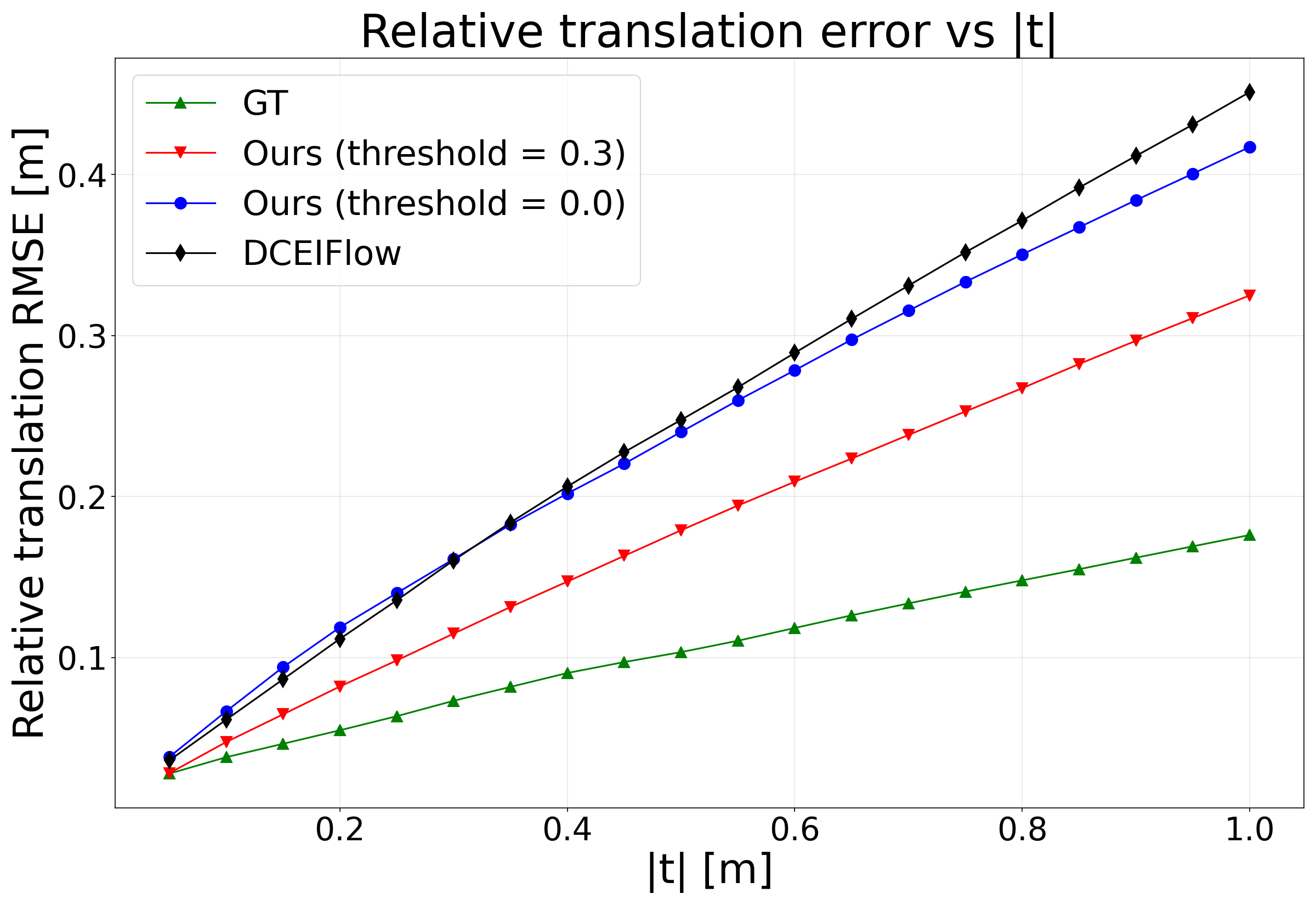

Figs.˜6(a) and 6(b) report relative translation and rotation RMSE as a function of translation magnitude . Applying a stricter confidence threshold (0.3 vs. 0.0) consistently reduces translation error across all motion magnitudes, with the gap growing as increases, confirming that the learned confidence reliably identifies high-quality flow estimates. The effect on rotation is more modest, as rotational motion is inherently harder to resolve from local observations alone. In both metrics, our method outperforms DCEIFlow, which relies on image frames in addition to events for dense flow estimation.