Quasinormal mode quantization of bound and propagating photons in complex lightguiding nanostructures for integrated devices

Abstract

Open optical or plasmonic resonators are placed on and connected through surfaces or via waveguides, forming complex lightguiding nanostructures, e.g. for integrated photonic quantum devices. We derive general boundary conditions for quasinormal modes that account for the structure’s specific geometry. We then present a general quantization scheme for multiple, interacting quasinormal-mode cavities coupled to quantum emitters and to a non-bosonic bath of propagating photons on waveguides or a surface. We derive a system-bath Hamiltonian with rigorously defined coupling elements that can be computed using Maxwell solvers, including light-matter coupling between the electromagnetic field and quantum emitters. We define system-bath correlation functions for an effective, bath-mediated, and time-delayed interaction between the quasinormal modes and quantum emitters, which is a main ingredient commonly used to simulate open quantum system dynamics.

Preprint

1 Introduction

Quantum emitters such as atoms, molecules, or quantum dots, coupled to the modes of optical cavities or plasmonic resonators, are fundamental building blocks of many quantum technologies [48, 52, 44, 65, 51, 3, 6, 35], and a must-have for integrated photonic circuits. While setups using resonators in homogeneous background media have limited applications in quantum information technologies, e.g., the transmission of entangled states between satellites [77, 76], many quantum technologies use multiple cavities in structured environments, such as waveguide-coupled cavities [13, 49, 51], for efficient intercavity coupling. See Fig. 1 for example structures of coupled cavities in different environments.

Theoretical treatments often start with a Hamiltonian or Lindbladian, where the cavity modes are assumed to be the orthonormal modes of closed resonators, while losses and coupling between different cavities are added heuristically [13, 5, 12]. Decay rates and coupling elements for realistic systems are not mostly defined in terms of modal properties and must be obtained elsewhere, e.g., by comparison to experiments.

In contrast, quasinormal modes (QNMs) are the solutions to the source-free Helmholtz equation with a complex permittivity (or dielectric function) under outgoing wave boundary conditions [41, 33, 58]. The QNMs have complex eigenfrequencies leading to temporal decay and spatial divergence outside the resonator caused by causality. This divergence can be addressed in a few-mode approximation by replacing the QNMs outside the resonator with regularized, frequency-dependent QNM fields, obtained from a Dyson scattering equation [24, 38]. Quasinormal modes have been used to study a variety of setups in optics and photonics, and yield accurate results, even for systems with significant losses [58, 71, 74, 53, 26, 40].

The construction of operators for quantized, quasi-bound QNMs has been performed for individual cavities [16] as well as coupled-cavity systems [18], including multi-cavity systems with significant retardation delays [21]. These quantum theories yield rigorously defined, numerically calculable coupling parameters that allow for the implementation of quantized QNMs into established methods for complex quantum dynamics [20, 37], such as the time-convolutionless (TCL) method [8], the hierarchical equations of motion (HEOM) [1, 67, 22], or path integral methods [9, 25, 10, 23]. However, previous work on quantized QNMs has focused on cavities in vacuum or homogeneous background media and is not immediately applicable to other environments. A rigorous quantized QNM theory for multiple coupled cavities in structured environments, such as waveguides or surfaces, is therefore needed.

Figure 1: Examples of different types of coupled QNM cavities separated by distance $R$ in various types of background structures. (a) Metal dimers described by a Drude permittivity $\epsilon_{M}$ in a 3D homogeneous background medium $\epsilon_{B}$ [38, 37]. (b) Cavities $V_{1},V_{2}$ on a photonic crystal with lattice constant $a$, side-coupled to the same periodic photonic crystal waveguide [28, 75, 31]. (c) Plasmonic nanoparticles $V_{1},V_{2}$ described by the Drude permittivity $\epsilon_{M}$ near a planar surface [73, 4].

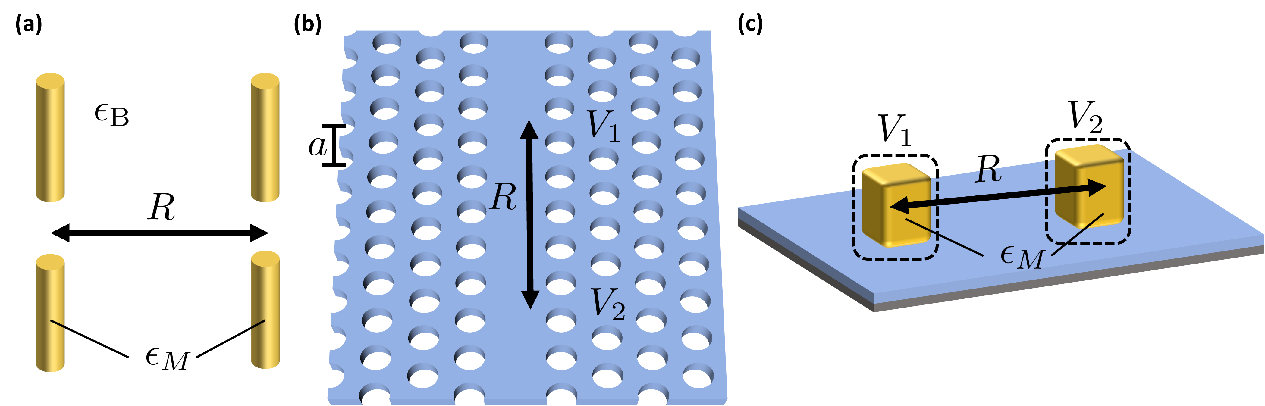
We present here a generalization of the quantization schemes for QNMs from Refs. [16, 21, 37] to structured background media, including waveguide-coupled cavities or cavities near surfaces. In Sec. 2, we derive general boundary conditions for the electric field, which also apply to the QNMs. From these general boundary conditions, we derive the specific boundary conditions for closed systems, systems in 1D, 2D, and 3D homogeneous background media (i.e., the Silver-Müller radiation condition [42, 61]), waveguide-coupled cavities [31], or cavities on surfaces. We also discuss the case of combined background structures, where different boundary conditions apply in different directions.

In Sec. 4, we discuss the classical theory of QNMs, their definition and their regularization (for use outside the cavity regions), and then introduce the adapted quantization scheme for cavities in different background. We discuss the overlap between the quasi-bound modes of separated cavities, that decreases exponentially with the cavity separation parameter, which acts as a measure for the separation between the cavities [21]. The QNM quantization naturally yields a set of non-bosonic bath operators that primarily describe photons propagating through the background medium between the cavities. We introduce the QNM system-bath Hamiltonian with rigorously defined eigenenergies and coupling parameters between the system and bath, as well as coupling to quantum emitters. As an example, we consider two-level systems (TLSs) that couple to the electric field via dipole coupling. We define coupling elements between the TLSs and the QNMs, respectively, to bath photons. The extension to multi-level emitters is straightforward.

Finally, in Sec. 5, we present the dynamics of the non-bosonic bath operators and define correlation functions for bath-mediated, time-delayed QNM-QNM, QNM-TLS, and TLS-TLS interactions, including coupling elements that are rigorously defined in terms of QNM parameters. These correlation functions can be implemented in many standard open quantum system dynamics schemes [67, 22, 69, 64, 56].

Table 1: Overview of the types of boundary conditions (BCs) in different dimensions and different kinds of lightguiding background structures.

BC	Section	Equation
General	2.2	(8)
Closed cavity	2.3	(2.3)
Free space 1D	2.4	(12)
Free space 2D	2.4	(2.4)
Free space 3D	2.4	(20)
Waveguide	2.5	(2.5)
Surfaces	3.1	(3.1),(3.1)
Multiple structures	3.2	(38)

2 Boundary conditions for cavities in structured media

2.1 Cavity modes in different background environments

We consider an absorptive, isotropic, inhomogeneous, and non-magnetic medium. The electric field in this medium solves the Helmholtz equation

$$\Big[\nabla\times\nabla\times-\frac{\omega^{2}}{c^{2}}\epsilon(\mathbf{r},\omega)\Big]\mathbf{E}(\mathbf{r},\omega)=i\omega\mu_{0}\mathbf{J}(\mathbf{r},\omega),$$ (1)

where $\epsilon(\mathbf{r},\omega)$ is the electric permittivity (or complex dielectric constant), and $\mathbf{J}(\mathbf{r},\omega)$ is the source current-density. Extensions to anisotropic or magnetic media are possible, see for example Ref. [32]. The field from Eq. (1) must also obey the correct boundary conditions (BCs) to match the specific geometry of the medium. The goal of this section is to derive BCs for the field in different kinds of environments.

If the system is an optical cavity or nanoplasmonic resonator in a lightguiding background medium (e.g., waveguides, surfaces, or free space), the field from Eq. (1) will be dominated by the resonances of the cavity. These resonances are described by the resonator modes, which solve the source-free Helmholtz equation at a specific eigenfrequency $\tilde{\omega}_{\mu}$:

$$\nabla\times\nabla\times\tilde{\mathbf{f}}_{\mu}(\mathbf{r})-\frac{\tilde{\omega}_{\mu}^{2}}{c^{2}}\epsilon(\mathbf{r},\tilde{\omega}_{\mu})\tilde{\mathbf{f}}_{\mu}(\mathbf{r})=0.$$ (2)

In an isolated system without absorption, the modes from Eq. (2) are the Hermitian normal modes, while for open boundary conditions, they are quasinormal modes (QNMs) with complex eigenfrequencies [36, 41, 33, 58]. For non-degenerate modes, the electric field near a specific resonance takes the form [2, 59]

$$\lim_{\omega\to\tilde{\omega}_{\mu}}(\omega-\tilde{\omega}_{\mu})\mathbf{E}(\mathbf{r},\omega)=\lim_{\omega\to\tilde{\omega}_{\mu}}a_{\mu}(\omega)\tilde{\mathbf{f}}_{\mu}(\mathbf{r}),$$ (3)

where $a_{\mu}(\omega)=(1/2i\epsilon_{0})\int\mathrm{d}^{3}r\tilde{\mathbf{f}}_{\mu}(\mathbf{r})\cdot\mathbf{J}(\mathbf{r},\omega)$ is an analytic expansion coefficient [32]. The boundary conditions derived below can be represented via a linear operator $\hat{L}(\mathbf{r},\omega)$ which generates the BCs for the electric field on a piecewise smooth surface $\mathcal{S}$ [e.g., Eq. (20)]. In this case,

$$\Big[\hat{L}(\mathbf{r},\omega)\mathbf{E}(\mathbf{r},\omega)\Big]_{\mathbf{r}\in\mathcal{S}}=0\to\Big[\hat{L}(\mathbf{r},\tilde{\omega}_{\mu})\tilde{\mathbf{f}}_{\mu}(\mathbf{r})\Big]_{\mathbf{r}\in\mathcal{S}}=0$$ (4)

relates the BCs for the electric field to the BCs of the QNMs.

2.2 General boundary condition

For a general formulation of the boundary conditions for the electric field from Eq. (1), we assume a volume $V$ bounded by a piecewise smooth surface $\mathcal{S}$. The electromagnetic Green’s function (or dyad) solves the Helmholtz equation (1) for a point-source,

$$\Big[\nabla\times\nabla\times-\frac{\omega^{2}}{c^{2}}\epsilon(\mathbf{r},\omega)\Big]\mathbf{G}(\mathbf{r},\mathbf{r}^{\prime},\omega)=\frac{\omega^{2}}{c^{2}}\mathbb{1}\delta(\mathbf{r}-\mathbf{r}^{\prime}),$$ (5)

where $\mathbb{1}$ is the unit dyad, and $\delta(\mathbf{r}-\mathbf{r}^{\prime})$ is the Dirac delta function. Towards the goal of deriving the boundary conditions on $\mathcal{S}$, we use Green’s second identity [17]:

$$\int_{V}\mathrm{d}^{3}r^{\prime}\Big\{\mathbf{G}^{T}(\mathbf{r}^{\prime},\mathbf{r},\omega)\cdot\big[\nabla_{r^{\prime}}\times\nabla_{r^{\prime}}\times\mathbf{E}(\mathbf{r}^{\prime},\omega)\big]-\mathbf{E}(\mathbf{r}^{\prime},\omega)\cdot\big[\nabla_{r^{\prime}}\times\nabla_{r^{\prime}}\times\mathbf{G}(\mathbf{r}^{\prime},\mathbf{r},\omega)\big]^{T}\Big\}$$

$$=\oint_{\mathcal{S}}\mathrm{d}A_{s}\hat{\mathbf{n}}_{s}\cdot\Big\{\mathbf{E}(\mathbf{s},\omega)\times\big[\nabla_{s}\times\mathbf{G}(\mathbf{s},\mathbf{r},\omega)\big]^{T}-\mathbf{G}^{T}(\mathbf{s},\mathbf{r},\omega)\times\big[\nabla_{s}\times\mathbf{E}(\mathbf{s},\omega)\big]\Big\},$$ (6)

where $\hat{\mathbf{n}}_{s}$ is the normal vector on $\mathcal{S}$, which points outwards with respect to $V$. We insert the Helmholtz equations for the electric field and Green’s function on the left-hand-side, and rearrange the terms to obtain the following expression for the full electric field in $V$:

$$\mathbf{E}(\mathbf{r},\omega) =\frac{i}{\omega\epsilon_{0}}\int_{V}\mathrm{d}^{3}r^{\prime}\mathbf{G}(\mathbf{r},\mathbf{r}^{\prime},\omega)\cdot\mathbf{J}(\mathbf{r}^{\prime},\omega)$$

$$-\frac{c^{2}}{\omega^{2}}\oint_{\mathcal{S}}\mathrm{d}A_{s}\hat{\mathbf{n}}_{s}\cdot\Big\{\mathbf{E}(\mathbf{s},\omega)\times\big[\nabla_{s}\times\mathbf{G}(\mathbf{s},\mathbf{r},\omega)\big]^{T}-\mathbf{G}^{T}(\mathbf{s},\mathbf{r},\omega)\times\big[\nabla_{s}\times\mathbf{E}(\mathbf{s},\omega)\big]\Big\}.$$ (7)

The first term on the right-hand side represents the field that is generated by sources within the volume, while the second term is the net flow of radiation through the surface $\mathcal{S}$, e.g., due to emitters or absorbers outside of $V$. If there is no flow through $\mathcal{S}$, e.g., for an isolated system or if $V$ covers the entire space, the integral over the outer surface $\mathcal{S}_{\rm out}$ of $V$ must vanish, yielding boundary conditions (BCs) for $\mathbf{E}(\mathbf{r},\omega)$ via

$$\oint_{\mathcal{S}_{\rm out}}\mathrm{d}A_{s}\hat{\mathbf{n}}_{s}\cdot\Big\{\mathbf{E}(\mathbf{s},\omega)\times\big[\nabla_{s}\times\mathbf{G}(\mathbf{s},\mathbf{r},\omega)\big]^{T}-\mathbf{G}^{T}(\mathbf{s},\mathbf{r},\omega)\times\big[\nabla_{s}\times\mathbf{E}(\mathbf{s},\omega)\big]\Big\}=0.$$ (8)

In what follows, we derive several well-known BCs from this integral. An overview of these BCs is given in Tab. 1. These boundary conditions can be used to numerically calculate the fields of resonators coupled to various lightguiding background structures. Using the relation from Eq. (3), they can be used to derive analytic BCs for the QNMs $\tilde{\mathbf{f}}_{\mu}(\mathbf{r})$ in various backgrounds.

2.3 Closed volume BC

A simple example is a finite volume $V$ with no holes and a closed boundary surface $\mathcal{S}_{\rm closed}$ as sketched in Fig. 2(a) for a scattering medium inside a closed resonator. The surface integral over $\mathcal{S}_{\rm closed}$ vanishes since no radiation can leave or enter $V$. Since we cannot assume anything about the Green’s function within $V$, the condition from Eq. (8) can only be fulfilled generally if

$$\hat{\mathbf{n}}_{s}\times\mathbf{E}(\mathbf{s},\omega)\big|_{s\in\mathcal{S}_{\rm closed}}=0,$$

$$\hat{\mathbf{n}}_{s}\times\big[\nabla\times\mathbf{E}(\mathbf{s},\omega)\big]\big|_{s\in\mathcal{S}_{\rm closed}}=0,$$ (9)

which are the usual boundary conditions on a surface with no external surface currents.

2.4 Homogeneous background media

Next, we consider a finite scattering geometry inside a volume $V_{\rm in}$ embedded in a homogeneous background medium $V_{\rm out}$, where $\epsilon(\mathbf{r},\omega)|_{r\in V_{\rm out}}=\epsilon_{B}$. We discuss this setup in one, two, and three dimensions (1D, 2D, 3D). We illustrate example structures together with the boundary conditions for all three cases in Fig. 2(b)-(d). In three dimensions, the outgoing boundary condition is the Silver-Müller radiation condition [42, 61], which is the typical choice for open cavity quasinormal modes in homogeneous media [32, 16, 21].

One Dimensional System. First, we consider a 1D structure embedded in a homogeneous background medium [Fig. 2(b)]. Such a setup can be achieved, for example, by a dielectric slab that is infinite in extent in the $y$-$z$ plane, so that equations reduce to their 1D equivalents along the $x$-axis. The 1D equivalent of Eq. (8) reads (Appendix A)

$$[E(x,\omega)\partial_{x}G(x,x^{\prime},\omega)-G(x^{\prime},x,\omega)\partial_{x}E(x,\omega)]_{x\to\pm\infty}=0,$$ (10)

where $x^{\prime}$ lies within the scattering volume, and $x$ lies in the very far field. This yields two boundary conditions, one to the left-hand side $x\to-\infty$, and one to the right-hand side $x\to+\infty$. We derive the boundary condition for $x\to+\infty$ here, the case for $x\to-\infty$ is obtained accordingly. In the far-field limit $x\gg x^{\prime}$, the Green’s function in Eq. (10) reduces to the Green’s function of a point source in a lossless homogeneous background medium, i.e., $G(x,x^{\prime},\omega)\to ik\exp[ik(x-x^{\prime})]/2$ [cf. Eq. (5)], where $k=n_{B}\omega/c$ is the wavenumber in the homogeneous background medium with refractive index $n_{B}=\sqrt{\epsilon_{B}}$. Hence, we obtain from Eq. (10),

$$\lim_{x\to\infty}\frac{ik}{2}\mathrm{e}^{ik(x-x^{\prime})}[ikE(x,\omega)-\partial_{x}E(x,\omega)]=0.$$ (11)

For a cavity with a clearly defined surface, such as a dielectric slab or open Fabry-Perot cavity, this far-field boundary condition is equivalent to the boundary condition at the cavity surface [cf. Fig. 2(b)]

$$[\partial_{x}E(x,\omega)-ikE(x,\omega)]_{x\searrow x_{R}}=0,$$ (12)

where $x_{R}$ is the right-hand side surface of the cavity [34, 32]. A similar boundary condition is obtained from the left-hand side limit $x\to-\infty$ and reads [cf. Fig. 2(b)],

$$[\partial_{x}E(x,\omega)+ikE(x,\omega)]_{x\nearrow x_{L}}=0,$$

where $x_{L}$ is the left-hand side surface of the cavity, which yields waves propagating away from the cavity in the other direction.

Two Dimensional System. Next, we consider a two-dimensional example, such as a 2D microdisk resonator [72, 18, 54] as sketched in Fig. 2(c). Here, we consider purely 2D phenomena in free space, while phenomena at a planar surface in 3D are considered in Sec. 3.1. The 2D equivalent of Eq. (8) reads (Appendix A),

$$\lim_{\rho\to\infty}\oint_{\mathcal{C}(\rho)}\mathrm{d}s\,\hat{\mathbf{e}}_{\rho}\cdot\Big\{\big[\nabla_{\bm{\rho}}\mathbf{G}(\bm{\rho},\mathbf{r},\omega)\big]^{T}\cdot\mathbf{E}(\bm{\rho},\omega)-\mathbf{G}^{T}(\bm{\rho},\mathbf{r},\omega)\cdot\big[\nabla_{\bm{\rho}}\mathbf{E}(\bm{\rho},\omega)\big]\Big\}=0,$$ (13)

where $\mathbf{r}\in V_{\rm in}$ lies in the scattering volume, while $\bm{\rho}=\rho\hat{\mathbf{e}}_{\rho}$ runs to the surrounding circular boundary $\mathcal{C}(\rho)$ with radius $\rho$ and outward pointing normal vector $\hat{\mathbf{e}}_{\rho}$ [Fig. 2(c)]. Furthermore, $\mathrm{d}s=\rho\,\mathrm{d}\varphi$ with $\varphi\in[0,2\pi)$.

Again, in the limit of a far-field boundary $\rho\to\infty$, the Green’s function reduces to the 2D free space Green’s function [39]

$$\mathbf{G}(\bm{\rho},\mathbf{r},\omega)\to\frac{ik^{2}}{4\epsilon_{B}}H^{(1)}_{0}(ks)\mathbb{1},$$ (14)

where $\mathbb{1}$ is the unit dyadic, again $k=n_{B}\omega/c$, and $H^{(1)}_{0}(ks)$ is the zero-th Hankel function of the first kind. Also, $s=|\bm{\rho}-\mathbf{r}|$, since, in a homogeneous medium, the Green’s function depends only on the distance between two points. In the limit $ks\to\infty$ (which follows from $\rho\to\infty$), the Hankel function tends to $H^{(1)}_{0}(ks)\to\sqrt{2/(\pi ks)}\mathrm{e}^{iks-i\pi/4}$ [39]. Since $\rho\gg|\mathbf{r}|$, we approximate $s\approx\rho$ everywhere except in the exponential. Hence, Eq. (13) reduces to

$$0=\lim_{\rho\to\infty} \int_{0}^{2\pi}\mathrm{d}\varphi\frac{i\sqrt{2k^{3}}\mathrm{e}^{iks-i\pi/4}}{4\epsilon_{B}}\sqrt{\rho}\Big\{\left(ik-\frac{1}{2\rho}\right)\mathbf{E}(\bm{\rho},\omega)-\hat{\mathbf{e}}_{\rho}\cdot\big[\nabla_{\bm{\rho}}\mathbf{E}(\bm{\rho},\omega)\big]\Big\}.$$ (15)

This expression vanishes if [cf. Fig. 2(c)]

$$\lim_{\rho\to\infty}\sqrt{\rho}\,\mathbf{E}(\bm{\rho},\omega)\quad\mathrm{finite},\quad{\rm and}$$

$$\lim_{\rho\to\infty}\sqrt{\rho}\,\Big\{ik\mathbf{E}(\bm{\rho},\omega)-\hat{\mathbf{e}}_{\rho}\cdot\big[\nabla_{\bm{\rho}}\mathbf{E}(\bm{\rho},\omega)\big]\Big\}=0,$$ (16)

which constitute the outgoing wave boundary conditions in 2D.

Three Dimensional System: Silver-Müller radiation condition. For a cavity in a three-dimensional homogeneous background medium, we use for the outer boundary a spherical surface $\mathcal{S}(R)$ with radius $R$, as sketched in Fig. 2(d). Since, in the limit $R\to\infty$  no sources are outside the volume, the condition from Eq. (8) applies. In the far-field limit, the scattering geometry behaves like a point source, so that the full Green’s function becomes the transverse Green’s function of the homogeneous background

$$\lim_{R\to\infty}\mathbf{G}(\mathbf{r},\mathbf{R},\omega)\to\frac{\omega^{2}}{c^{2}}\frac{\mathrm{e}^{iks}}{4\pi s}\left(\mathbb{1}-\hat{\mathbf{s}}\otimes\hat{\mathbf{s}}\right),$$ (17)

where $\mathbf{s}=\mathbf{r}-\mathbf{R}$, $s=|\mathbf{s}|$, and $\hat{\mathbf{s}}=\mathbf{s}/s$. Here, $\mathbf{r}\in V_{\rm in}$, and $\mathbf{R}$ runs to the outer surface $\mathcal{S}(R)$. Together with Eq. (8), we obtain

$$0=\lim_{R\to\infty}\oint_{\mathcal{S}(R)}\mathrm{d}A\,\frac{\mathrm{e}^{iks}}{4\pi s}\Big\{\left(ik-\frac{1}{s}\right)\left[\mathbf{E}(\mathbf{R},\omega)\times(\mathbb{1}\times\hat{\mathbf{s}})\right]-\left(\mathbb{1}-\hat{\mathbf{s}}\otimes\hat{\mathbf{s}}\right)\times\left[\nabla\times\mathbf{E}(\mathbf{R},\omega)\right]\Big\}\cdot\hat{\mathbf{R}},$$ (18)

where $\hat{\mathbf{R}}=\mathbf{R}/|\mathbf{R}|$ is the normal vector on $\mathcal{S}(R)$. Now, we set $\mathbf{s}\approx\mathbf{R}$, everywhere except in the exponential, and perform a far-field approximation, where $|\mathbf{R}|\gg|\mathbf{r}|$. We furthermore rewrite the integral into an integral over the solid angle $\Omega$ via $\mathrm{d}A=R^{2}\mathrm{d}\Omega$. We then find

$$\lim_{R\to\infty}\int_{\Omega}\mathrm{d}\Omega\frac{\mathrm{e}^{iks}}{4\pi}\Big[R\big\{ik\mathbf{E}^{T}(\mathbf{R},\omega)+\hat{\mathbf{R}}\times\big[\nabla\times\mathbf{E}^{T}(\mathbf{R},\omega)\big]\big\}-\mathbf{E}^{T}(\mathbf{R},\omega)\Big]=0.$$ (19)

Figure 2: (a) Closed cavity system. A scattering medium described by permittivity $\epsilon(\mathbf{r},\omega)$ is placed inside a closed resonator of length $L$, so that waves will scatter back from the resonator surface, described by the boundary conditions in Eq. (2.3). (b)-(d) Cavity in a homogeneous background medium for 1D, 2D, and 3D, respectively. In 1D, the condition from Eq. (10) yields outgoing boundary conditions at the cavity surface [Eq. (12)]. For 2D (3D), we choose a circular (spherical) far-field surface for the integral from Eq. (13) [Eq. (8)], which yields the outgoing wave boundary conditions from Eq. (2.4) [Eq. (20)].

The condition is satisfied if the relations are fulfilled [cf. Fig. 2(d)]

$$\lim_{R\to\infty}R\,\mathbf{E}^{T}(\mathbf{R},\omega)\,\,\mathrm{finite},\quad{\rm and}$$

$$\lim_{R\to\infty}R\left\{ik\mathbf{E}^{T}(\mathbf{R},\omega)+\hat{\mathbf{R}}\times\left[\nabla\times\mathbf{E}^{T}(\mathbf{R},\omega)\right]\right\}=0,$$

which constitute the Silver-Müller radiation condition [61, 42]. They can be combined into the single expression [32]

$$\hat{\mathbf{R}}\times\left[\nabla\times\mathbf{E}^{T}(\mathbf{R},\omega)\right]\to-ik\mathbf{E}^{T}(\mathbf{R},\omega),\,R\to\infty.$$ (20)

Note that the radiation condition applies to the transverse part of the electric field only. Since $\nabla\times\mathbf{E}^{L}=0$ holds, the longitudinal part $\mathbf{E}^{L}$ reads [cf. Eq. (1)]

$$\mathbf{E}^{L}(\mathbf{r},\omega)=\frac{-i}{\omega\epsilon_{0}}\frac{\mathbf{J}^{L}(\mathbf{r},\omega)}{\epsilon(\mathbf{r},\omega)}.$$ (21)

2.5 Waveguide radiation condition

In this section, we want to derive the boundary conditions that apply to the field of a cavity coupled to a lossless waveguide. (cf. Fig. 3) We assume that the waveguide constitutes the only loss channel to the cavity, i.e., no energy leaks into the surrounding medium. We consider a finite-size scattering geometry (e.g., an optical cavity) centered at $z=0$ coupled to an infinite, non-absorptive waveguide as sketched in Fig. 3(b), or a periodic photonic crystal waveguide as in Fig. 1(b). The waveguide has modes $\mathbf{f}_{kj}(\mathbf{r})=\mathbf{e}_{kj}(\mathbf{r})\mathrm{e}^{ik_{j}z}$, where $k_{j}$ is the $j$-th mode index (propagation constant) at wavenumber $k=\omega/c$, which is obtained from the eigenvalue equation for the modes [63]. The modes $\mathbf{f}_{kj}$ propagate forwards or backward in the direction of the waveguide. We assume $k_{j}>0$ so that $\mathbf{f}_{kj}(\mathbf{r})$ is a forward-propagating mode and $\mathbf{f}_{-kj}(\mathbf{r})\equiv\mathbf{f}^{*}_{kj}(\mathbf{r})$ is a backward-propagating mode.

Meanwhile, we assume that the mode functions $\mathbf{e}_{kj}(\mathbf{r})$ decay exponentially perpendicular to the waveguide (or are zero outside if the waveguide cladding is perfectly reflecting). For a periodic waveguide (e.g., on a photonic crystal) with lattice constant $a$, $\mathbf{e}_{kj}(\mathbf{r})=\mathbf{e}_{kj}(\mathbf{r}+a\hat{\mathbf{e}}_{z})$ are Bloch modes, which are normalized across the unit cell [27, 31].

Generally, the waveguide modes $\mathbf{f}_{kj}(\mathbf{r})$ are normalized according to [31, 63]

$$\int_{A_{\infty}}\mathrm{d}A\,\hat{\mathbf{n}}\cdot \Big\{\mathbf{f}_{kj}(\mathbf{s})\times\big[\nabla\times\mathbf{f}^{*}_{k^{\prime}j^{\prime}}(\mathbf{s})\big]+\mathbf{f}^{*}_{k^{\prime}j^{\prime}}(\mathbf{s})\times\big[\nabla\times\mathbf{f}_{kj}(\mathbf{s})\big]\Big\}=\delta_{jj^{\prime}}\delta_{kk^{\prime}},$$ (22)

where $A_{\infty}$ is the infinite cross-section of the waveguide [Fig. 3(a)], and $\hat{\mathbf{n}}$ is the normal surface vector on $A_{\infty}$, parallel to the waveguide axis. Note that for an infinite waveguide, the position of the cross-section along the $z$-axis is arbitrary.

Next, we consider a far-field cylindrical surface $\mathcal{S}_{\infty}=\mathcal{S}_{\rm side}\cup\mathcal{S}_{-}\cup\mathcal{S}_{+}$ around the waveguide and cavity, where $\mathcal{S}_{\rm side}$ is the side of the cylinder, while $\mathcal{S}_{-}$ and $\mathcal{S}_{+}$ are the bases of the cylinder in the negative and positive $z$-directions, respectively [see Fig. 3(b) for a sketch of the far-field surface]. In the limit of an infinite cylinder, there are no sources outside the far-field surface $\mathcal{S}_{\infty}$, and Eq. (8) applies. Similar to the derivation in homogeneous background media, the full Green’s function in the far-field limit can be expanded in terms of the waveguide modes with propagation constants $k_{j}$ at frequency $\omega$ [27]

$$\mathbf{G}(\mathbf{r},\mathbf{r}^{\prime},\omega)\to\sum_{j}A_{kj} \Big[\mathbf{f}_{kj}(\mathbf{r})\mathbf{f}^{*}_{kj}(\mathbf{r}^{\prime})\Theta(z-z^{\prime})+\mathbf{f}^{*}_{kj}(\mathbf{r})\mathbf{f}_{kj}(\mathbf{r}^{\prime})\Theta(z^{\prime}-z)\Big],$$ (23)

where $A_{kj}=ia\omega/(2k_{j})$, where $a$ is the lattice constant for a periodic waveguide, and $a=1$ for a continuous waveguide. For practical calculations, an integration over the dispersion of the bound modes is often carried out, so that, instead of many modes $j$ at wavenumber $k$, Eq. (23) is expressed via a single mode $k_{\omega}$. In this case, $A_{k}=ia\omega/(2v_{g})$, where $v_{g}$ is the group velocity [27, 31].

We insert the Green’s function in the far-field limit into Eq. (8):

$$0=\sum_{j}A_{kj}\mathbf{f}_{kj}(\mathbf{r})\int_{\mathcal{S}_{-}}\mathrm{d}A\,\hat{\mathbf{n}}\cdot\Big\{\mathbf{E}(\mathbf{s},\omega)\times\big[\nabla\times\mathbf{f}_{kj}^{*}(\mathbf{s})\big]-\mathbf{f}_{kj}^{*}(\mathbf{s})\times\big[\nabla\times\mathbf{E}(\mathbf{s},\omega)\big]\Big\}$$

$$+\sum_{j}A_{kj}\mathbf{f}^{*}_{kj}(\mathbf{r})\int_{\mathcal{S}_{+}}\mathrm{d}A\,\hat{\mathbf{n}}\cdot\Big\{\mathbf{E}(\mathbf{s},\omega)\times\big[\nabla\times\mathbf{f}_{kj}(\mathbf{s})\big]-\mathbf{f}_{kj}(\mathbf{s})\times\big[\nabla\times\mathbf{E}(\mathbf{s},\omega)\big]\Big\}.$$ (24)

Figure 3: (a) Sketch of a single cylindrical waveguide with forward (backward) propagating waveguide modes $\mathbf{f}^{(*)}_{kj}(\mathbf{r})$ and infinite cross-section $A_{\infty}$ over which the normalization of the waveguide modes is carried out [Eq. (22)]. (b) Sketch of a cavity coupled to the waveguide from (a) as its only loss channel. The field of the open cavity extends into the waveguide. Equation (8) is evaluated over a far-field surface $\mathcal{S}_{\rm side}\cup\mathcal{S}_{-}\cup\mathcal{S}_{+}$, yielding the waveguide boundary conditions from Eq. (2.5).

The integral over the lateral surface of the cylinder vanishes because the lossless waveguide modes are assumed decay exponentially in that direction. From the normalization condition of the waveguide modes in Eq. (22), it follows that Eq. (2.5) holds for

$$\mathbf{E}(\mathbf{r},\omega) \to\sum_{j}\sigma^{\rm backw}_{kj}\mathbf{f}^{*}_{kj}(\mathbf{r}),\,z\to-\infty,$$

$$\mathbf{E}(\mathbf{r},\omega) \to\sum_{j}\sigma^{\rm forw}_{kj}\mathbf{f}_{kj}(\mathbf{r}),\,z\to\infty,$$ (25)

i.e., the field far away to the left of the scatterer is represented by the left-propagating waveguide modes only, and the field far away to the right is represented by the right-propagating modes only. Here,

$$\sigma^{\rm backw}_{kj}=\int_{A_{\infty}}\mathrm{d}A\,\hat{\mathbf{n}}\cdot\Big\{\mathbf{E}(\mathbf{s},\omega)\times\big[\nabla\times\mathbf{f}_{kj}(\mathbf{s})\big]-\mathbf{f}_{kj}(\mathbf{s})\times\big[\nabla\times\mathbf{E}(\mathbf{s},\omega)\big]\Big\},$$

$$\sigma^{\rm forw}_{kj}=\int_{A_{\infty}}\mathrm{d}A\,\hat{\mathbf{n}}\cdot\Big\{\mathbf{E}(\mathbf{s},\omega)\times\big[\nabla\times\mathbf{f}_{kj}^{*}(\mathbf{s})\big]-\mathbf{f}_{kj}^{*}(\mathbf{s})\times\big[\nabla\times\mathbf{E}(\mathbf{s},\omega)\big]\Big\}$$ (26)

are the projections of the field onto the left-propagating and right-propagating waveguide modes, respectively. Note that, for $z\to\pm\infty$ only waveguide modes with real $k_{j}$ contribute, since the modes with $\mathrm{Im}(k_{j})>0$ are damped to zero.

The equations in Eq. (2.5) constitute the boundary conditions for the electric field of a cavity coupled to an infinite waveguide as its only loss channel and hold in this form also for periodic waveguides, e.g., on a photonic crystal [31]. The boundary conditions demand that the field far away from the scatterer can be represented by the waveguide modes traveling away from the scatterer, thus fulfilling the condition that there is no backscattering from outside $\mathcal{S}_{\infty}$.

3 Boundary conditions for combinations of multiple lightguiding structures

After deriving specific boundary conditions for setups in which the cavity emission enters a single type of guiding background structure, we now turn to setups in which the boundary conditions vary with the direction of emission. As a first example, we discuss a cavity near the interface between layered media, where the far-field emission can appear as either spherical waves in free space or bound surface waves. We formulate the boundary condition integral from Eq. (8) for this case, which is dominated by the spherical waves or surface waves, depending on the direction of the emission. As our second example, we consider a cavity coupled to multiple waveguides simultaneously. Here, we formulate conditions under which the waveguides can be treated as separate background structures so that far-field emissions into one of the waveguides take the form of outward propagating waveguide modes of that waveguide only.

3.1 Cavities at planar surfaces

We start with a cavity near a planar interface between media, as sketched in Fig. 4. For a simple example, we consider the case with a single interface between homogeneous media, so that the permittivity reads $\epsilon(z)=\Theta(z)\epsilon_{1}+\Theta(-z)\epsilon_{2}$ with $\epsilon_{1}\neq\epsilon_{2}$. Extensions to layered media are possible [70, 4]. Such setups are common in nano-optics, where cavities or quantum emitters (atoms, molecules, or quantum dots) are located on substrate surfaces [73, 59]. For a simple illustration, we consider a finite-size cavity above the interface centered at $\mathbf{r}\approx 0$. We also focus only on the region $z\geq 0$ and do not discuss the transmitted fields below the interface, which can be treated similarly, accounting for the different material properties for $z<0$.

Theoretical treatments of such systems are usually based on one of two approaches: Numerical treatments, including the calculation of QNMs for these setups, use perfectly matched layers that surround the cavity and substrate to use fictious far-field losses to simulate open boundary conditions [73, 4]. Meanwhile, treatments based on analytic approaches use a partial spatial Fourier transform of the Green’s function and fields in the plane parallel to the interface and then describe the reflections at the interface in terms of Fresnel coefficients [62, 47, 45]. These analytic expressions of the Green’s function take the form of Sommerfeld integrals [62, 45, 47],

$$\mathbf{G}(\rho,z,\omega)\big|_{z>0}=k^{2}\int_{0}^{\infty}\mathrm{d}\kappa\frac{\kappa}{q_{1}}\mathbf{K}(\rho,\kappa,\omega)\mathrm{e}^{iq_{1}z},$$ (27)

where $q_{j}=\sqrt{\epsilon_{j}k^{2}-\kappa^{2}}$ is the z-component of the wave vector in the j-th medium, which is an implicit function of $k=\omega/c$ and $\kappa$. Furthermore, the dyadic kernel $\mathbf{K}$ (see Appendix B for the definition) depends on Bessel functions $J_{n}(\kappa\rho)$, which account for the lateral wave part, and the Fresnel coefficients [45]

$$r_{s}(\kappa)=\frac{q_{1}-q_{2}}{q_{1}+q_{2}},\quad r_{p}(\kappa)=\frac{\epsilon_{2}q_{1}-\epsilon_{1}q_{2}}{\epsilon_{2}q_{1}+\epsilon_{1}q_{2}}.$$ (28)

Inserting Eq. (27) into the boundary integral from Eq. (8) does not immediately yield an analytic expression of the far-field boundary conditions for the electric field. For such an expression, the Green’s function in real space is required. However, for the boundary conditions, we only require the asymptotic Green’s function in the limit $r=\sqrt{\rho^{2}+z^{2}}\to\infty$. We therefore neglect all contributions that decay faster than $1/r$.

The Sommerfeld integral from Eq. (27) contains a pole at $\kappa=\sqrt{\epsilon_{1}}k$ from the $1/q_{1}$-term. It can be formally separated into propagating contributions $\kappa\leq\sqrt{\epsilon_{1}}k$ (and therefore $q_{1}\geq 0$), and evanescent contributions $\kappa>\sqrt{\epsilon_{1}}k$, where $q_{1}$ is imaginary with positive imaginary part, leading to exponential decay. For $z\to\infty$, the evanescent contributions vanish, and we obtain a purely propagating solution in free space in terms of spherical waves [45]

$$\mathbf{G}(\rho,z,\omega)\big|_{z\to\infty}\approx\mathbf{G}_{\rm free}(\rho,z,\omega)=\frac{k^{2}e^{ikr}}{4\pi r}\big[(\mathbb{1}-\hat{\mathbf{e}}_{r}\hat{\mathbf{e}}_{r})+\mathbf{A}^{\rm ref}(\theta)\big],$$ (29)

where the $\mathbb{1}-\hat{\mathbf{e}}_{r}\hat{\mathbf{e}}_{r}$ yields the transverse free space Green’s function (sec. 2.4), and $\mathbf{A}^{\rm ref}(\theta)$ (see Appendix B for the analytic form) yields the reflected contributions. The reflections depend on the incident angle $\theta$ between $\mathbf{r}$ and the $z$-axis, and hence $\sin(\theta)=\rho/r,\,\cos(\theta)=z/r$. In the limit $z\to 0$ ($\theta\to\pi/2$), $\mathbf{A}^{\rm ref}(\pi/2)\to-(\mathbb{1}-\hat{\mathbf{e}}_{r}\hat{\mathbf{e}}_{r})$ so that $\mathbf{G}_{\rm free}(\rho,z,\omega)|_{z\to 0}\approx 0$. Physically, this vanishing of the free space contribution to the Green’s function accounts for destructive interference between the free space emission and reflections as the wave propagates almost parallel to the interface.

For finite $z$ (and especially $z\to 0$), the evanescent contributions to Eq. (27) cannot be neglected. Since the free space contributions vanish in this limit, the dominant contributions to the Green’s function near the surface generally decay faster than $1/r$ [30, 46, 15], and are therefore neglected here in our discussion of asymptotic behavior. However, the Fresnel coefficient $r_{p}(\kappa)$ has an additional pole if $q_{1}=-(\epsilon_{1}/\epsilon_{2})q_{2}$. This can be achieved for $\epsilon_{2}<0<\epsilon_{1}<|\epsilon_{2}|$ if [45]

$$\kappa^{2}=\kappa_{\rm spp}^{2}=k^{2}\frac{\epsilon_{1}\epsilon_{2}}{\epsilon_{1}+\epsilon_{2}},$$ (30)

which is the lateral wavenumber of a surface plasmon polariton. Since $\kappa_{\rm spp}>k$, $q_{1}(\kappa_{\rm spp})\equiv iq_{\rm spp}$ is imaginary, so that this surface wave decays exponentially perpendicular to the interface and vanishes for $z\to\infty$. For our discussion here, we assume that the setup from Fig. 4 supports surface plasmon polaritons, which dominate in the far field near the surface over other contributions.

Unlike the propagating free space waves, the propagation of the surface wave is confined to the interface and therefore scales as $1/\sqrt{\rho}$. This can be seen by considering the evanescent part of the Sommerfeld integral from Eq. (27) for the limit $\rho\to\infty,z\to 0$. We only consider the contributions to the dyadic $\mathbf{K}$ which contain the Fresnel coefficient $r_{p}(\kappa)$ which has a pole at $\kappa=\kappa_{\rm spp}$. We assume that all other contributions to the Green’s function in the limit $\rho\to\infty,z\to 0$ decay faster than $1/r$. The Bessel functions $J_{n}(\kappa\rho)$ in $\mathbf{K}$ in the limit $\rho\to\infty$ scale as

$$J_{n}(\kappa\rho)\big|_{\rho\to\infty}\approx\sqrt{\frac{1}{2\pi\kappa\rho}}\left(\mathrm{e}^{i\kappa\rho-in\pi/2-i\pi/4}+\mathrm{e}^{-i\kappa\rho+in\pi/2+i\pi/4}\right).$$ (31)

We only include the retarded contribution, yielding an overall scaling of $\mathrm{e}^{i\kappa\rho}/\sqrt{\kappa\rho}$ from the Bessel function. Hence, the Green’s function approximately reads,

$$\mathbf{G}(\rho,z,\omega)\big|_{\rho\to\infty,z\to 0}\approx k^{2}\int_{\sqrt{\epsilon_{1}}k}^{\infty}\mathrm{d}\kappa\frac{\kappa}{q_{1}}\tilde{\mathbf{K}}^{p}(\kappa,\omega)\frac{\mathrm{e}^{i\kappa\rho}}{\sqrt{\kappa\rho}}\frac{\mathrm{e}^{iq_{1}z}}{\epsilon_{2}q_{1}+\epsilon_{1}q_{2}}.$$ (32)

Here, the dyadic $\tilde{\mathbf{K}}^{p}(\kappa,\omega)$ contains additional $\kappa$-dependent contributions as well as prefactors from the Bessel functions, which we leave general here, since they do not factor into the boundary conditions below. Assuming that all contributions (except the pole at $\kappa=\kappa_{\rm spp}$) are analytic, we can solve the integral via contour integral methods. Towards this, we shift the pole to $\kappa=\kappa_{\rm spp}+i\eta$, with $\eta>0$, since we are interested in the retarded solution. In the limit $\eta\to 0$, the original pole is recovered. Then, we integrate over the path shown in Fig. 4(c), where the integrals over the paths $C_{2}$ and $C_{3}$ vanish, since the exponential $\mathrm{e}^{i\kappa\rho}$ goes to zero in the limit $\rho\to\infty$ for any $\kappa$ with positive imaginary part. Thus, the red path $C_{1}+C_{2}+C_{3}$ in Fig. 4(c) for $t\to\infty$ recovers the integral from Eq. (32). Evaluating the expression at the pole and then setting $\eta\to 0$ yields

$$\mathbf{G}(\rho,z,\omega)\big|_{\rho\to\infty,z\to 0}\approx\mathbf{G}_{\rm sur}(\rho,z,\omega)=\mathbf{B}(\kappa_{\rm spp},\omega)\frac{\mathrm{e}^{i\kappa_{\rm spp}\rho}}{\sqrt{\rho}}\mathrm{e}^{-q_{\rm spp}z},$$ (33)

where again, we left the dyadic $\mathbf{B}(\kappa_{\rm spp},\omega)$ general, since it does not factor into the boundary conditions below. We merely note that the shape of $\mathbf{B}(\kappa_{\rm spp},\omega)$ is such that the Green’s function remains transverse: $\nabla\cdot\mathbf{G}_{\rm sur}=0$.

Hence, this setup presents a combination of two different cases discussed above in Sec. 2.4: For $z\to\infty$, the freely propagating and reflected fields take the form of spherical waves, similar to the 3D free space case. Meanwhile, depending on the ratio between $\epsilon_{1}$ and $\epsilon_{2}$, bound surface states may appear for $\rho\to\infty$ and finite $z$, which behave like the 2D waves with an additional exponential decay perpendicular to the interface. Assuming that all other contributions decay faster that $1/r$, we can write the asymptotic Green’s function as a simple sum of these two contributions:

$$\mathbf{G}(\rho,z,\omega)|_{r\to\infty}\approx\mathbf{G}_{\rm free}(\rho,z,\omega)+\mathbf{G}_{\rm sur}(\rho,z,\omega),$$ (34)

where $\mathbf{G}_{\rm free}$ vanishes as we approach the surface, while $\mathbf{G}_{\rm sur}$ vanishes as we move way from the surface. Thus, the two contributions represent two different regimes depending on the direction of the emission from the cavity. We note that the neglected higher order terms could in principle also be included in the Green’s function and may even play a crucial role for cases without bound surface states, where they constitute the dominant contribution to lateral emissions from the cavity.

Figure 4: Sketch of a cavity (here, a plasmonic particle) located near the planar interface between two different media $\epsilon_{1}\neq\epsilon_{2}$. (a) As our far-field surface for the boundary condition integral from Eq. (8), we chose a half sphere with radius $R\to\infty$. The far field takes different forms, depending on the direction in which the emission occurs. Far away from the surface, the waves behave like spherical waves the form $\mathrm{e}^{i\kappa_{\rm spp}r}/\sqrt{r}$ (red arrow) appear, similar to the 2D problem from Sec. 2.4. Here, $\kappa_{\rm spp}$ is the in-plane wavenumber of a surface plasmon polarition [cf. Eq. (30)]. (b) Same as before but with a cylindrical far-field surface with height $h\to\infty$ and radius $\rho\to\infty$. (c) Integration path to calculate the integral from Eq. (32). The integrals over the paths $C_{2}$ and $C_{3}$ vanish in the limit $\rho\to\infty$, since there, ${\rm Im}(\kappa)>0$. Thus, the integration over the full path $C_{1}+C_{2}+C_{3}$ recovers the integral from Eq. (32) in the limit $t\to\infty$. Setting $\eta\to 0$ after the integration yields the result from Eq. (33).

Inserting Eq. (34) into the boundary integral from Eq. (8), we obtain, for $z>0$,

$$\oint_{\mathcal{S}_{\rm out}}\mathrm{d}A_{s}\hat{\mathbf{n}}_{s}\cdot\Big[ \mathbf{E}(\mathbf{s},\omega)\times\big\{\nabla_{s}\times\big[\mathbf{G}_{\rm free}(\rho,z,\omega)+\mathbf{G}_{\rm sur}(\rho,z,\omega)\big]\big\}^{T}$$

$$-\big[\mathbf{G}_{\rm free}^{T}(\rho,z,\omega)+\mathbf{G}_{\rm sur}^{T}(\rho,z,\omega)\big]\times\big\{\nabla_{s}\times\mathbf{E}(\mathbf{s},\omega)\big\}\Big]=0,$$ (35)

where we set the position of the source $\mathbf{r}\approx 0$, and $\rho,z$ are the in-plane and out-of-plane components of $\mathbf{s}$, respectively. Since the free space spherical waves and surface waves are different phenomena, the Green’s functions $\mathbf{G}_{\rm free}$ and $\mathbf{G}_{\rm sur}$ are linearly independent, and the two contributions to Eq. (3.1) must vanish independently. For the far-field outer surface $\mathcal{S}_{\rm out}$, we may choose any appropriate surface that matches the geometry of the waves. Indeed, we can even choose different far-field surfaces for each of the two contributions to simplify the derivation.

For the free space part, we choose a semi-spherical surface with radius $R\to\infty$ in the upper half space $z>0$ [cf. Fig. 4(a)]. For this surface, $\mathrm{d}A_{s}=R^{2}\mathrm{d}\Omega$, where $\Omega$ is the solid angle of the half sphere. Thus, the resulting boundary conditions take a similar shape as the Silver-Müller radiation condition from Eq. (20), except that we must distinguish between the polarization directions to account for the reflection (see Appendix B for the derivation):

$$\lim_{R\to\infty}R\hat{\mathbf{e}}_{\varphi}\cdot\left\{\hat{\mathbf{e}}_{r}\times[\nabla\times\mathbf{E}(\mathbf{R},\omega)]-\hat{\mathbf{e}}_{r}\times\Big[\frac{\nabla r_{s}(\theta)}{1+r_{s}(\theta)}\times\mathbf{E}(\mathbf{R},\omega)\Big]+ik\mathbf{E}(\mathbf{R},\omega)\right\}=0,\quad{\rm and}$$

$$\lim_{R\to\infty}R\hat{\mathbf{e}}_{\theta}\cdot\left\{\hat{\mathbf{e}}_{r}\times[\nabla\times\mathbf{E}(\mathbf{R},\omega)]+\mathbf{E}(\mathbf{R},\omega)\left[ik-\hat{\mathbf{e}}_{\theta}\cdot\frac{\nabla\sin(2\theta)r_{p}(\theta)}{1-\cos(2\theta)r_{p}(\theta)}\right]\right\}=0,$$ (36)

where $\hat{\mathbf{e}}_{r},\hat{\mathbf{e}}_{\theta},\hat{\mathbf{e}}_{\varphi}$ are the unit vectors in spherical coordinates, and $r_{s}(\theta),r_{p}(\theta)$ are the Fresnel coefficients from Eq. (28) in real space, which depend on the incident angle $\theta$ between $\mathbf{R}=R\hat{\mathbf{e}}_{r}$ and the $z$-axis. Without reflection, Eq. (3.1) recovers the Silver-Müller radiation condition from Eq. (20).

For the surface plasmon part, we instead use a cylindrical far-field surface with radius $\rho\to\infty$ and height $h\to\infty$ [Fig. 4(b)]. The integral from Eq. (3.1) for the surface wave part thus separates into an integral over the top of the cylinder at $z=h\to\infty$, where the Green’s function $\mathbf{G}_{\rm sur}$ is zero, and an integral over the side of the cylinder, where $\mathrm{d}A_{s}=\rho\mathrm{d}\varphi\mathrm{d}z$. Thus, we obtain (cf. Appendix B) for the surface waves:

$$\lim_{\rho\to\infty}\sqrt{\rho}\mathbf{E}(\mathbf{r},\omega)\,{\rm finite},\quad{\rm and},$$

$$\lim_{\rho\to\infty}\sqrt{\rho}\left\{i\mathbf{k}_{\rm spp}\times[\hat{\mathbf{e}}_{\rho}\times\mathbf{E}(\mathbf{r},\omega)]-\hat{\mathbf{e}}_{\rho}\times[\nabla\times\mathbf{E}(\mathbf{r},\omega)]\right\}=0,$$ (37)

where $\mathbf{k}_{\rm spp}=\kappa_{\rm spp}\hat{\mathbf{e}}_{\rho}+iq_{\rm spp}\hat{\mathbf{e}}_{z}$ is the wavevector of the surface plasmon polariton, so that the exponential decay of the field in the $z$-direction follows from the boundary conditions. If we restrict ourselves to the regime immediately at the surface $z\to 0$, we find the familiar Silver-Müller form [cf. Eq. (20)]: $\lim_{\rho\to\infty}\sqrt{\rho}[i\kappa_{\rm spp}\mathbf{E}+\hat{\mathbf{e}}_{\rho}\times(\nabla\times\mathbf{E})]=0$.

Thus, the far-field behavior of the electric field depends on whether the emission occurs into free space or along the interface. For a setup of multiple cavities on a substrate that supports surface waves [cf. Fig. 1(c)], propagation along the surface offers a more efficient transfer of energy between the cavities than propagation through free space, since the surface waves decay as $1/\sqrt{r}$ instead of $1/r$.

3.2 Combination of multiple lightguiding structures

As our second example, we consider a cavity coupled to multiple, non-intersecting waveguides in different directions, as sketched in Fig. 5. Our goal is to derive a measure for when the different background structures (here, the separate waveguides) can be treated separately when deriving the boundary conditions. Before discussing the example system below, we introduce a generalized formulation. We assume that the background volume $V_{\rm out}=\cup_{\alpha}V_{\rm out}^{\alpha}$ separates into a finite number of continuous volumes $V_{\rm out}^{\alpha}$ which each contain a part of the background structure, e.g., a waveguide, surface, or free space. Then, the outer surface surrounding the whole structure (scatterer+background) $\mathcal{S}_{\rm out}=\cup_{\alpha}\mathcal{S}_{\rm out}^{\alpha}$ separates into a finite number of piecewise smooth surfaces, where $\mathcal{S}_{\rm out}^{\alpha}=\mathcal{S}_{\rm out}\cap V_{\rm out}^{\alpha}$ (e.g., the different waveguide cross-sections in Fig. 5). Thus, we separate the integral from Eq. (8) into a sum of integrals that account for losses through the different loss channels:

$$0=\sum_{\alpha}\int_{\mathcal{S}_{\rm out}^{\alpha}}\mathrm{d}A_{s} \hat{\mathbf{n}}_{s}\cdot\Big\{\mathbf{E}(\mathbf{s},\omega)\times\big[\nabla_{s}\times\mathbf{G}(\mathbf{s},\mathbf{r},\omega)\big]^{T}-\mathbf{G}(\mathbf{r},\mathbf{s},\omega)\times\big[\nabla_{s}\times\mathbf{E}(\mathbf{s},\omega)\big]\Big\}.$$ (38)

Since each integral accounts for losses through a different part of the background structure (and is typically connected to a different direction or separated connecting structure), we assume that the different $\mathcal{S}_{\rm out}^{\alpha}$-integrals vanish independently, yielding separate boundary conditions for the cavity field in the different directions. Next, using a Dyson scattering equation similar to the one derived in Appendix C (see also Refs. [24, 38]), we write, for $\mathbf{s}\in\mathcal{S}^{\alpha}_{\rm out}$:

$$\mathbf{G}(\mathbf{r},\mathbf{s},\omega)=\mathbf{G}^{\alpha}(\mathbf{r},\mathbf{s},\omega)+\Delta\mathbf{G}(\mathbf{r},\mathbf{s},\omega),$$ (39)

where $\mathbf{G}^{\alpha}(\mathbf{r},\mathbf{s},\omega)$ is the Green’s function for the background structure $\alpha$ alone (e.g., just a single waveguide, surface, or free space) and

$$\Delta\mathbf{G}(\mathbf{r},\mathbf{s},\omega)=\int_{\overline{V}^{\alpha}_{\rm out}}\mathrm{d}^{3}r^{\prime}[\epsilon(\mathbf{r},\omega)-\epsilon^{\alpha}(\mathbf{r},\omega)]\mathbf{G}(\mathbf{r},\mathbf{r}^{\prime},\omega)\cdot\mathbf{G}^{\alpha}(\mathbf{r}^{\prime},\mathbf{s},\omega)$$ (40)

is the difference between the full Green’s function and the contribution from background structure $\alpha$ only. Here, $\epsilon^{\alpha}(\mathbf{r},\omega)$ is the permittivity for background structure $\alpha$ only, and $\overline{V}^{\alpha}_{\rm out}$ is the complement of the background volume $V^{\alpha}_{\rm out}$. Hence, it follows from Eq. (40) that this difference is small if the Green’s function $\mathbf{G}^{\alpha}(\mathbf{r}^{\prime},\mathbf{s},\omega)$ is small for positions $\mathbf{r}^{\prime}\notin V_{\rm out}^{\alpha}$. For example, if $\alpha$ denotes a single waveguide and the relevant modes of the waveguide used to expand the Green’s function $\mathbf{G}^{\alpha}$ decay fast perpendicular to the waveguide, $\Delta\mathbf{G}$ will be small, and the full Green’s function in the $\mathcal{S}^{\alpha}_{\rm out}$-integral can be approximated via the Green’s function for that part of the background structure only.

For a simple example, we consider the structure sketched in Fig. 5 of a cavity coupled to three different semi-finite waveguides. The waveguides can be different in shape, material, or core refractive index, and hence support different waveguide modes. For illustrative purposes, we assume that no emission from the cavity into the surrounding free space occurs; instead, all emissions enter one of the three waveguides, depending on the direction of emission. We also assume lossless waveguides with modes that decay exponentially in the direction perpendicular to the waveguide axis. Hence, in Eq. (38), $\alpha=1,2,3$, denoting the three different waveguides, and $\mathcal{S}^{1/2/3}_{\rm out}$ are the far-field infinite cross-sections of the waveguides. Since the waveguide modes decay exponentially perpendicularly to the waveguide axis, $\Delta\mathbf{G}\approx 0$ in Eq. (40), and, for the integral over each of the cross-sections, we can (approximately) expand the Green’s function from Eq. (38) in terms of the waveguide modes of that waveguide only. Consequently, three different boundary conditions apply to the cavity field, depending on the direction of emission. The emitted field far away from the cavity takes the shape of the outward propagating waveguide modes of only that waveguide into which the emission occurs [cf. Eq. (2.5)]

$$\mathbf{E}(\mathbf{r},\omega)\big|_{\mathbf{r}\in V_{\rm out}^{\alpha}} \to\sum_{j}\sigma^{\alpha}_{kj}\mathbf{f}^{\alpha}_{kj}(\mathbf{r}),\,\mathbf{r}\to\infty,$$ (41)

where $\mathbf{f}^{\alpha}_{kj}(\mathbf{r})$ is the waveguide mode of the $\alpha$-th waveguide and $\sigma^{\alpha}_{kj}$ is the expansion coefficient from Eq. (2.5).

Thus, combinations of different types of background structures can be computed approximately, if $\Delta\mathbf{G}\approx 0$, via separate boundary integrals for the different kinds of lightguiding background media. This way, knowledge of the full background Green’s function is not necessary to obtain an approximation of the far-field behavior of the cavity field.

Figure 5: Example for a system with separate background structures. A cavity is coupled to three semi-finite waveguides with different refractive indices $n_{1/2/3}$. The waveguides can be made from different materials or have different cross-section profiles, thereby supporting very different waveguide modes (indicated by the different colors). If the waveguide modes do not extend into the outside medium [$\Delta\mathbf{G}\approx 0$, cf. Eq. (40)], the three waveguides can be treated separately and the cavity emission inside one of the waveguides obeys the boundary conditions for that waveguide alone [Eq. (2.5)]. Here, $\mathcal{S}^{1/2/3}_{\rm out}$ are the far-field infinite cross-sections through the different waveguides, used for obtaining the boundary conditions, as shown in Sec. 2.5.

4 Multi-cavity quasinormal modes in the presence of guiding structures

Having discussed the derivation of boundary conditions for the field of a resonator embedded in a specific type of background structure (or combination of background structures), we now move on to the multi-cavity theory. We consider multiple optical cavities or nanoplasmonic resonators in a general background medium. The full permittivity reads,

$$\epsilon(\mathbf{r},\omega)=\epsilon_{\rm back}(\mathbf{r},\omega)+\Delta\epsilon(\mathbf{r},\omega)\sum_{i}\chi_{V_{i}}(\mathbf{r}),$$ (42)

where $\epsilon_{\rm back}(\mathbf{r},\omega)$ is the permittivity of the background medium, and $\Delta\epsilon(\mathbf{r},\omega)=\epsilon(\mathbf{r},\omega)-\epsilon_{\rm back}(\mathbf{r},\omega)$ is the perturbation of the permittivity from the background value due to the presence of the cavity. Furthermore, $\chi_{V_{i}}(\mathbf{r})$ is unity inside the cavity volume $\mathbf{r}\in V_{i}$ and zero elsewhere. For generality, we assume here a frequency-dependent background permittivity, which (in principle) can include absorption and dispersion. In practice, to enable the definition of QNMs, the absorption and dispersion must be weak enough so that there is negligible backscattering from the background to the cavity [11].

Instead of calculating joint QNMs for the entire multi-cavity structure (which is generally not feasible), we calculate the single-cavity QNMs $\tilde{\mathbf{f}}_{i_{\mu}}(\mathbf{r})$ from the source-free Helmholtz equation (2) using only the single-cavity permittivity $\epsilon^{(i)}(\mathbf{r},\omega)=\epsilon_{\rm back}(\mathbf{r},\omega)+\Delta\epsilon(\mathbf{r},\omega)\chi_{V_{i}}(\mathbf{r})$, where the permittivity is set to the background value at all other cavities. Multi-cavity properties such as the full electromagnetic Green’s function are then constructed from the single-cavity QNMs via a set of scattering equations, as discussed in Ref. [38]. The boundary conditions are obtained as described in the previous sections (cf. Tab. 1).

4.1 QNM regularization

The QNMs have complex eigenfrequencies $\tilde{\omega}_{i_{\mu}}=\omega_{i_{\mu}}-i\gamma_{i_{\mu}},\,\gamma_{i_{\mu}}>0$ so that the temporal decay of the cavity field is inherent to the mode. However, this causes the QNMs to diverge in the far field [41, 58, 32]. This is a straightforward consequence of causality, since the field at $r\to\infty$ must have been emitted at $t\to-\infty$, which, for a temporally decaying mode, leads to spatial divergence.

We address this divergence by adapting the QNM regularization approach to general background media. The approach yields frequency-dependent, non-diverging regularized QNM fields which account for propagation away from the resonator. These fields can be calculated via a Dyson scattering equation [24], or alternatively, via the field-equivalence principle (see Appendix C for a derivation) [20, 55]:

$$\tilde{\mathbf{F}}_{i_{\mu}}(\mathbf{r},\omega)=i\tilde{\omega}_{i_{\mu}}\mu_{0}\oint_{\mathcal{S}_{i}}\mathrm{d}A_{s}\mathbf{G}_{\rm back}(\mathbf{r},\mathbf{s},\omega)\cdot\tilde{\mathbf{J}}_{i_{\mu}}(\mathbf{s})-\oint_{\mathcal{S}_{i}}\mathrm{d}A_{s}\tilde{\mathbf{M}}_{i_{\mu}}(\mathbf{s})\cdot\Big[\nabla\times\mathbf{G}_{\rm back}(\mathbf{s},\mathbf{r},\omega)\Big],$$ (43)

where [55]

$$\tilde{\mathbf{J}}_{i_{\mu}}(\mathbf{s})=\hat{\mathbf{n}}_{s}\times\nabla\times\tilde{\mathbf{f}}_{i_{\mu}}(\mathbf{s})/(i\tilde{\omega}_{i_{\mu}}\mu_{0}),\quad\tilde{\mathbf{M}}_{i_{\mu}}(\mathbf{s})=-\hat{\mathbf{n}}_{s}\times\tilde{\mathbf{f}}_{i_{\mu}}(\mathbf{s}),$$ (44)

are the electric and magnetic surface currents generated by the QNM $i_{\mu}$ on the cavity surface $\mathcal{S}_{i}$ of $V_{i}$, and $\hat{\mathbf{n}}_{s}$ is the surface normal vector, pointing outwards with respect to $V_{i}$.

The presence of the background Green’s function $\mathbf{G}_{\rm back}$ in Eq. (43) ensures that the shape of the outward propagating regularized QNM field matches the specific geometry of the background, e.g., propagation through a waveguide or along a surface. For combined background guiding structures as discussed in Sec. 3.2, The shape of the regularized QNM is different within the different background media. Similar to Sec. 3.2, we separate the outside volume into different parts containing the different lightguiding background structures $V_{\rm out}=\cup_{\alpha}V_{\rm out}^{\alpha}$. We furthermore denote by $\mathcal{S}_{i}^{\alpha}$ that part of the cavity surface $\mathcal{S}_{i}$ through which energy is radiated into the background structure $V_{\rm out}^{\alpha}$. Then, for $\mathbf{r}\in V_{\rm out}^{\alpha}$ (and sufficiently far away from the cavity), the regularized QNM field can be approximately written as:

$$\tilde{\mathbf{F}}_{i_{\mu}}(\mathbf{r},\omega)\big|_{\mathbf{r}\in V_{\rm out}^{\alpha}}\approx i\tilde{\omega}_{i_{\mu}}\mu_{0}\oint_{\mathcal{S}^{\alpha}_{i}}\mathrm{d}A_{s}\mathbf{G}^{\alpha}(\mathbf{r},\mathbf{s},\omega)\cdot\tilde{\mathbf{J}}_{i_{\mu}}(\mathbf{s})-\oint_{\mathcal{S}^{\alpha}_{i}}\mathrm{d}A_{s}\tilde{\mathbf{M}}_{i_{\mu}}(\mathbf{s})\cdot\Big[\nabla\times\mathbf{G}_{\rm back}(\mathbf{s},\mathbf{r},\omega)\Big],$$ (45)

where $\mathbf{G}^{\alpha}$ is again the background Green’s function for the type of lightguiding structure in $V_{\rm out}^{\alpha}$ only. Equation (45) allows for an efficient approximation of the regularized fields in complex environments.

4.2 QNM quantization

For general dissipative, dispersive, non-magnetic media, the electric field operator reads [14, 66, 50]

$$\hat{\mathbf{E}}(\mathbf{r},\omega)=i\sqrt{\frac{\hbar}{\pi\epsilon_{0}}}\int\mathrm{d}^{3}r^{\prime}\sqrt{\epsilon_{I}(\mathbf{r}^{\prime},\omega)}\mathbf{G}(\mathbf{r},\mathbf{r}^{\prime},\omega)\cdot\hat{\mathbf{b}}(\mathbf{r}^{\prime},\omega),$$ (46)

where $\epsilon_{I}(\mathbf{r},\omega)$ is the imaginary part of the permittivity, and $\hat{\mathbf{b}}(\mathbf{r},\omega)$ are bosonic photon operators with continuous spatial and frequency indices, i.e.,

$$\left[\hat{b}_{p}(\mathbf{r},\omega),\hat{b}^{\dagger}_{q}(\mathbf{r}^{\prime},\omega^{\prime})\right]=\delta_{pq}\delta(\mathbf{r}-\mathbf{r}^{\prime})\delta(\omega-\omega^{\prime}).$$ (47)

The full electromagnetic field Hamiltonian can be diagonalized to read [14, 66, 50],

$$H=\hbar\int_{0}^{\infty}\mathrm{d}\omega\int\mathrm{d}^{3}r\omega\hat{\mathbf{b}}^{\dagger}(\mathbf{r},\omega)\cdot\hat{\mathbf{b}}(\mathbf{r},\omega),$$ (48)

and the frequency-independent field operator is obtained via integration over all frequencies $\hat{\mathbf{E}}(\mathbf{r})=\int_{0}^{\infty}\mathrm{d}\omega\hat{\mathbf{E}}(\mathbf{r},\omega){+}\mathrm{H.a.}$

The bosonic photon operators $\hat{\mathbf{b}}(\mathbf{r},\omega)$ quantize the entire electromagnetic field. To obtain operators for the discrete QNMs of a single cavity only, we perform a projection onto the QNM subspace via [20, 21, 37]

$$\hat{a}_{i_{\mu}}=\int_{0}^{\infty}\mathrm{d}\omega\int\mathrm{d}^{3}r\mathbf{L}_{i_{\mu}}(\mathbf{r},\omega)\cdot\hat{\mathbf{b}}(\mathbf{r},\omega),$$ (49)

where the QNM projector kernels $\mathbf{L}_{i_{\mu}}(\mathbf{r},\omega)$ read,

$$\mathbf{L}_{i_{\mu}}(\mathbf{r},\omega)=\sum_{\nu}\left(S^{-1/2}\right)_{i_{\mu}i_{\nu}}\sqrt{\frac{2}{\pi\omega_{i_{\nu}}}}A_{i_{\nu}}(\omega)\Big[\chi_{V_{i}}(\mathbf{r})\sqrt{\epsilon_{I}(\mathbf{r},\omega)}\tilde{\mathbf{f}}_{i_{\nu}}(\mathbf{r})$$

$$+\chi_{\overline{V_{i}}}(\mathbf{r})\sqrt{\epsilon_{{\rm back},I}(\mathbf{r},\omega)}\tilde{\mathbf{F}}_{i_{\nu}}(\mathbf{r},\omega)\Big].$$ (50)

Here, $A_{i_{\nu}}(\omega)=\omega/[2(\tilde{\omega}_{i_{\nu}}-\omega)]$, and $\chi_{V}(\mathbf{r})$ is unity if $\mathbf{r}\in V$ and zero elsewhere. Hence, the QNMs $\tilde{\mathbf{f}}_{i_{\nu}}(\mathbf{r})$ are replaced with the regularized QNM fields $\tilde{\mathbf{F}}_{i_{\nu}}(\mathbf{r},\omega)$ for positions outside the cavity, and the imaginary part of the full permittivity $\epsilon_{I}(\mathbf{r},\omega)$ is replaced with the imaginary part of the background permittivity $\epsilon_{{\rm back},I}(\mathbf{r},\omega)$ so that only sources from within the cavity enter the projector, while sources from other cavities are removed. Furthermore, $\left(S^{-1/2}\right)_{i_{\mu}i_{\nu}}$ is the inverse square root of the intracavity overlap matrix defined in Appendix D.

From the definition of the QNM operators $\hat{a}_{i_{\mu}}$ in Eq. (49) together with the commutator of the operators $\hat{\mathbf{b}}(\mathbf{r},\omega)$ from Eq. (47), it follows that

$$[\hat{a}_{i_{\mu}},\hat{a}^{\dagger}_{j_{\nu}}] =\sum_{\mu^{\prime}\nu^{\prime}}\left(S^{-1/2}\right)_{i_{\mu}i_{\mu^{\prime}}}S_{i_{\mu^{\prime}}j_{\nu^{\prime}}}\left(S^{-1/2}\right)_{j_{\nu^{\prime}}j_{\nu}}=\delta_{ij}\delta_{\mu\nu}+(1-\delta_{ij})\tilde{S}^{\rm inter}_{i_{\mu}j_{\nu}},$$ (51)

where $S_{i_{\mu}j_{\nu}}=\delta_{ij}S^{\rm intra}_{i_{\mu}i_{\nu}}+(1-\delta_{ij})S^{\rm inter}_{i_{\mu}j_{\nu}}$ is the QNM overlap matrix, which separates into intra- and intercavity overlap. The overlap matrices are defined in Appendix D.

Due to the spatial separation of the cavities, the relative intercavity overlap $\tilde{S}^{\rm inter}_{i_{\mu}j_{\nu}}$ in Eq. (51) is exponentially small [21]

$$\tilde{S}^{\rm inter}_{i_{\mu}j_{\nu}}=\sum_{\mu^{\prime}\nu^{\prime}}\left(S^{-1/2}\right)_{i_{\mu}i_{\mu^{\prime}}}S^{\rm inter}_{i_{\mu^{\prime}}j_{\nu^{\prime}}}\left(S^{-1/2}\right)_{j_{\nu^{\prime}}j_{\nu}}\sim\mathrm{e}^{-P_{i_{\mu}j_{\nu}}},$$ (52)

where we defined a quantitative measure for the separation, the cavity separation parameter [21] (see Appendix E for the derivation of the generalization)

$$P_{i_{\mu}j_{\nu}}=\gamma^{\min}_{i_{\mu}j_{\nu}}\tau_{ij}+T^{\min}_{i_{\mu}j_{\nu}}.$$ (53)

The terms contributing to the cavity separation parameter reflect distinct properties of the QNMs. In the first term, $\gamma^{\min}_{i_{\mu}j_{\nu}}=\min[\gamma_{i_{\mu}},\gamma_{j_{\nu}}]$, and $\tau_{ij}=\Lambda_{ij}/c$ is the photon retardation time along the shortest optical path $\Lambda_{ij}$ between the cavity centers [7]. The optical path length is known from the integral $\Lambda_{ij}=\int_{\mathcal{C}_{ij}}\mathrm{d}s\,n(s)=\overline{n}|\mathcal{C}_{ij}|$ [7], where $\mathcal{C}_{ij}$ is the path of length $|\mathcal{C}_{ij}|$ between the centers of cavities $i$ and $j$ (e.g., along the center of a waveguide), and $n(s)$ is the refractive index with average $\overline{n}$ along the path. This contribution to $P_{i_{\mu}j_{\nu}}$ shows that the quantized QNMs are quasi-bound in the sense that they are mostly localized at their respective cavity and their overlap with modes from other cavities decreases exponentially with the distance [21].

In the second term, $T^{\rm min}_{i_{\mu}j_{\nu}}=\min[T_{i_{\mu},j_{\nu}},T_{j_{\nu},i_{\mu}}]$, where $T_{i_{\mu},j_{\nu}}=-\mathrm{ln}[U^{i}_{j_{\nu}}/U^{\rm tot}_{j_{\nu}}]$ is the transfer factor, which describes the transferred power $U^{i}_{j_{\nu}}$ to cavity $i$ from mode $j_{\nu}$ as a fraction of the total power $U^{\rm tot}_{j_{\nu}}$ radiated from mode $j_{\nu}$.

For certain setups and geometries, additional aspects of the mode may enter the cavity separation parameter. For example, the overlap also vanishes in the limit of very high-quality modes (cf. Appendix E). However, we do not consider these aspects in the following general discussion.

Therefore, for a large separation, i.e., $P_{i_{\mu}j_{\nu}}\gg 0$, the operators of the different cavities commute [cf. Eq. (51)], allowing the construction of Fock states for the individual cavities. For small separations, hybridized modes or coupled QNM theory must be used instead [68, 18, 54].

4.3 The QNM Hamiltonian

For well-separated cavities, the construction of QNM operators from Eq. (49) yields bosonic operators for the quantized QNMs of the individual cavities. However, the integration over all frequencies in Eq. (49) fixes the phase of the quantized QNMs, leading to modes that are quasi-bound, with propagation effects largely removed.

From the operator projection in Eq. (49) together with the commutator in Eq. (51), it follows that the operators $\hat{\mathbf{b}}(\mathbf{r},\omega)$ can be decomposed into QNM and non-QNM contributions via

$$\hat{\mathbf{b}}(\mathbf{r},\omega)=\sum_{i,\mu}\mathbf{L}^{*}_{i_{\mu}}(\mathbf{r},\omega)\hat{a}_{i_{\mu}}+\hat{\mathbf{c}}(\mathbf{r},\omega).$$ (54)

Here, we introduced bath operators $\hat{\mathbf{c}}(\mathbf{r},\omega)$ that are orthogonal to the QNM projector kernels $\mathbf{L}_{i_{\mu}}(\mathbf{r},\omega)$ so that QNM and bath operators commute [20, 21, 37]. Thus, the bath operators are mainly responsible for the propagation of photons through the background medium (the bath), and are generally non-bosonic [see Eq. (57)].

Using this decomposition, we bring the electromagnetic field Hamiltonian from Eq. (48) into system-bath form [20, 21]

$$H=H_{S}+H_{B}+H_{SB} =\hbar\sum_{i,\mu\eta}\left(\int_{0}^{\infty}\mathrm{d}\omega\int\mathrm{d}^{3}r\,\omega\,\mathbf{L}_{i_{\mu}}(\mathbf{r},\omega)\cdot\mathbf{L}^{*}_{i_{\eta}}(\mathbf{r},\omega)\right)\hat{a}^{\dagger}_{i_{\mu}}\hat{a}_{i_{\eta}}$$

$$\quad+\hbar\int_{0}^{\infty}\mathrm{d}\omega\int\mathrm{d}^{3}r\,\omega\,\hat{\mathbf{c}}^{\dagger}(\mathbf{r},\omega)\cdot\hat{\mathbf{c}}(\mathbf{r},\omega)$$

$$\quad+\hbar\sum_{i,\mu}\int_{0}^{\infty}\mathrm{d}\omega\int\mathrm{d}^{3}r\,\mathbf{g}_{i_{\mu}}(\mathbf{r},\omega)\cdot\hat{\mathbf{c}}(\mathbf{r},\omega)\,\hat{a}_{i_{\mu}}^{\dagger}{+}\mathrm{H.a.},$$ (55)

where [20, 21, 37]

$$\mathbf{g}_{i_{\mu}}(\mathbf{r},\omega)=\sum_{\nu}(\delta_{\mu\nu}\omega-\chi_{i_{\mu}i_{\nu}})\mathbf{L}_{i_{\nu}}(\mathbf{r},\omega)$$ (56)

is a noise-coupling element associated with a broad frequency bandwidth, and $\chi_{i_{\mu}i_{\nu}}=\sum_{\eta}(S^{-1/2})_{i_{\mu}i_{\eta}}\tilde{\omega}_{i_{\eta}}(S^{1/2})_{i_{\eta}i_{\nu}}$ is the symmetrized QNM eigenfrequency.

Note that, due to the assumption of a negligible overlap (large separation $P_{i_{\mu}j_{\eta}}\gg 0$), there is no direct coupling between the QNMs of different cavities in the system part. Instead, the QNMs of all cavities couple to the same bath of propagating photons. In a time-dependent theory, we thus obtain effective, time-delayed coupling between the different cavities via photon propagation through the background medium (cf. Sec. 5). While such coupling is generally weak in free space, the use of guiding structures, such as waveguides or plasmonic surfaces, can lead to significant coupling between separated systems in quantum technologies.

4.4 Bath operators for separate background structures

The bath operators are defined implicitly from Eq. (54), and therefore obey the non-bosonic commutation relation [20],

$$\left[\hat{c}_{p}(\mathbf{r},\omega),\hat{c}^{\dagger}_{q}(\mathbf{r}^{\prime},\omega^{\prime})\right]_{-} =\delta_{pq}\delta(\mathbf{r}-\mathbf{r}^{\prime})\delta(\omega-\omega^{\prime})-\sum_{k,\mu}L^{*}_{k_{\mu},p}(\mathbf{r},\omega)L_{k_{\mu},q}(\mathbf{r}^{\prime},\omega^{\prime}),$$ (57)

where the second term on the right-hand side represents the completeness relation on the quantized QNM subspace, which is here removed from the full-space $\delta$-function.

In a complex structure consisting of multiple emitters and different kinds of background structures (cf. Sec. 3), the bath operators may be separated into a sum of operators

$$\hat{\mathbf{c}}(\mathbf{r},\omega)=\sum_{\alpha}\chi_{V_{\rm out}^{\alpha}}(\mathbf{r})\hat{\mathbf{c}}^{\alpha}(\mathbf{r},\omega),$$ (58)

where the index $\alpha$ refers to the $\alpha$-th background structure as in Sec. 3. Then, the commutator from Eq. (57) decomposes into two different cases. Firstly $\mathbf{r},\mathbf{r}^{\prime}\in V_{\rm out}^{\alpha}$, where:

$$\left[\hat{c}_{p}(\mathbf{r},\omega),\hat{c}^{\dagger}_{q}(\mathbf{r}^{\prime},\omega^{\prime})\right]_{-}\big|_{\mathbf{r},\mathbf{r}^{\prime}\in V_{\rm out}^{\alpha}} =\left[\hat{c}_{p}^{\alpha}(\mathbf{r},\omega),\hat{c}^{\alpha,\dagger}_{q}(\mathbf{r}^{\prime},\omega^{\prime})\right]_{-}$$

$$=\delta_{pq}\delta(\mathbf{r}-\mathbf{r}^{\prime})\delta(\omega-\omega^{\prime})-\sum_{k,\mu}L^{*}_{k_{\mu},p}(\mathbf{r},\omega)L_{k_{\mu},q}(\mathbf{r}^{\prime},\omega^{\prime}).$$ (59)

Alternatively, if $\mathbf{r}\in V_{\rm out}^{\alpha},\mathbf{r}^{\prime}\in V_{\rm out}^{\beta},\,\alpha\neq\beta$, we find:

$$\left[\hat{c}_{p}(\mathbf{r},\omega),\hat{c}^{\dagger}_{q}(\mathbf{r}^{\prime},\omega^{\prime})\right]_{-}\big|_{\mathbf{r}\in V_{\rm out}^{\alpha},\mathbf{r}^{\prime}\in V_{\rm out}^{\beta}}^{\alpha\neq\beta}=\left[\hat{c}_{p}^{\alpha}(\mathbf{r},\omega),\hat{c}^{\beta,\dagger}_{q}(\mathbf{r}^{\prime},\omega^{\prime})\right]_{-}=-\sum_{k,\mu}L^{*}_{k_{\mu},p}(\mathbf{r},\omega)L_{k_{\mu},q}(\mathbf{r}^{\prime},\omega^{\prime}).$$ (60)

Since the quasi-bound QNMs are (mostly) confined to their cavity, the commutator in Eq. (60) (approximately) vanishes if the background structures are separated, e.g., two non-intersecting waveguides. In this case, the bath operators separate into a sum of commuting operators for the different substructures. In the following, we use the full bath operators $\hat{\mathbf{c}}(\mathbf{r},\omega)$ instead of the separated bath operators $\hat{\mathbf{c}}^{\alpha}(\mathbf{r},\omega)$ for generality.

4.5 Coupling of quantized QNMs to quantum emitters

Many quantum technologies are based on quantum emitters coupled to electromagnetic modes, e.g., an atom in an optical microcavity or near a plasmonic nanoparticle. We use two-level systems (TLSs) to model the quantum emitters. The extension to multi-level emitters is straightforward.

The TLSs couple to the electric field via dipole coupling, so that the TLS Hamiltonian reads

$$H^{\rm TLS} =\hbar\sum_{m}\omega_{m}\hat{\sigma}_{m}^{+}\hat{\sigma}_{m}-\sum_{m}\hat{\sigma}_{m}^{+}\int_{0}^{\infty}\mathrm{d}\omega\mathbf{d}_{m}\cdot\hat{\mathbf{E}}(\mathbf{r}_{m},\omega){-}\mathrm{H.a.},$$ (61)

where $\hat{\sigma}_{m}^{+}$ creates an excitation with energy $\hbar\omega_{m}$ in TLS $m$, and $\mathbf{d}_{m}$ is the dipole moment of TLS $m$ coupled to the electric field operator from Eq. (46) at the location $\mathrm{r}_{m}$. Accordingly, $\hat{\sigma}_{m}^{-}$ annihilates an excitation in TLS $m$.

Using Eq. (46) together with the decomposition of the operators $\hat{\mathbf{b}}(\mathbf{r},\omega)$ from Eq. (54), we bring the electric field operator into system-bath form:

$$\hat{\mathbf{E}}(\mathbf{r},\omega)=\sum_{i,\mu}\mathbf{E}_{i_{\mu}}(\mathbf{r},\omega)\hat{a}_{i_{\mu}}+i\sqrt{\frac{\hbar}{\epsilon_{0}\pi}}\int\mathrm{d}^{3}r^{\prime}\sqrt{\epsilon_{I}(\mathbf{r}^{\prime},\omega)}\mathbf{G}(\mathbf{r},\mathbf{r}^{\prime},\omega)\cdot\hat{\mathbf{c}}(\mathbf{r}^{\prime},\omega),$$ (62)

where we defined the QNM-generated electric field [37]

$$\mathbf{E}_{i_{\mu}}(\mathbf{r},\omega)=\frac{i}{\omega\epsilon_{0}}\int\mathrm{d}^{3}r^{\prime}\mathbf{G}(\mathbf{r},\mathbf{r}^{\prime},\omega)\cdot\mathbf{j}_{i_{\mu}}(\mathbf{r}^{\prime},\omega)$$ (63)

with the (classical) current density generated by the QNM, $\mathbf{j}_{i_{\mu}}(\mathbf{r},\omega)=\omega\sqrt{\frac{\hbar\epsilon_{0}}{\pi}\epsilon_{I}(\mathbf{r},\omega)}\mathbf{L}^{*}_{i_{\mu}}(\mathbf{r},\omega)$. The physical interpretation of the QNM-generated electric field is straightforward: The presence of the dissipative QNM creates a noise current that acts as a source of an electric field that a TLS interacts with. The QNM-generated electric field can be calculated numerically from a Helmholtz equation [cf. Eq. (1)] using $\mathbf{j}_{i_{\mu}}(\mathbf{r},\omega)$ as a source term. A more efficient approach uses the expansion of the Green’s function in terms of the single-cavity QNMs to obtain an expression of the electric field in terms of few dominant QNMs [38].

Thus, with Eq. (62), the Hamiltonian from Eq. (61) can be brought into system-bath form, where the TLSs and quasi-bound quantized QNMs act as the system and the propagating photons in the background lightguiding structure act as a bath. Thus, with a system-bath Hamiltonian and coupling parameters that are rigorously defined in terms of numerically calculable QNM parameters, we can perform quantum dynamics calculations for multi-cavity systems and quantum emitters in structured environments using this QNM framework.

5 System-bath correlation functions

System-bath correlation functions play a central role in many established open quantum system dynamics methods, such as Nakajima-Zwanzig equations [43, 78, 8] or the time-convolutionless approach (TCL) [60, 8] as well as in path integral approaches [9, 25, 10, 23], including the hierarchical equations of motion (HEOM) [1, 67, 22]. Therefore, in the following sections, we derive multicavity correlation functions with rigorously defined coupling parameters to characterize QNM-QNM, QNM-TLS, and TLS-TLS interactions in structured media.

The correlation functions considered here are of the form

$$C_{\mathbb{x}\mathbb{y}}(t,t^{\prime})=\sum_{pq}\int\mathrm{d}^{3}r\int_{0}^{\infty}\mathrm{d}\omega\int\mathrm{d}^{3}r^{\prime}\int_{0}^{\infty}\mathrm{d}\omega^{\prime}g_{\mathbb{x},p}(\mathbf{r},\omega)g^{*}_{\mathbb{y},q}(\mathbf{r}^{\prime},\omega^{\prime})\mathrm{tr}_{B}\left[\hat{c}_{p}(\mathbf{r},\omega,t)\hat{c}^{\dagger}_{q}(\mathbf{r}^{\prime},\omega^{\prime},t^{\prime})\rho_{B}\right].$$ (64)

Here, $\mathbb{x},\mathbb{y}$ are generic placeholder indices for the QNM or TLS indices [37], while $\mathrm{tr}_{B}[...]$ is the trace over the bath degrees of freedom, and $\rho_{B}=|{\rm vac}\rangle\langle{\rm vac}|$ is the initial vacuum bath state. Under the assumption of an initial vacuum bath state, it follows that

$$\mathrm{tr}_{B}\left[\hat{c}_{p}(\mathbf{r},\omega,t)\hat{c}^{\dagger}_{q}(\mathbf{r}^{\prime},\omega^{\prime},t^{\prime})\rho_{B}\right]=\left[\hat{c}_{p}(\mathbf{r},\omega,t),\hat{c}^{\dagger}_{q}(\mathbf{r}^{\prime},\omega^{\prime},t^{\prime})\right]_{-},$$

which we employ in the derivation of the specific correlation functions below.

5.1 Bath dynamics

To derive the correlation function from Eq. (64), we need the dynamics of the bath operators with respect to the bath Hamiltonian [cf. Eq. (4.3)]

$$H_{B}=\hbar\int_{0}^{\infty}\mathrm{d}\omega\int\mathrm{d}^{3}r\,\omega\hat{\mathbf{c}}^{\dagger}(\mathbf{r},\omega)\cdot\hat{\mathbf{c}}(\mathbf{r},\omega).$$ (65)

A detailed derivation of the bath dynamics was given in Ref. [37] in the context of cavities in a homogeneous three-dimensional background medium. The derivation of the time evolution of the bath operators for other environments follows the same steps, but with a different permittivity function and a different definition of the QNM projector kernels [Eq. (4.2)]. The time-dependent bath operators thus read,

$$\hat{\mathbf{c}}(\mathbf{r},\omega,t) =\hat{\mathbf{c}}(\mathbf{r},\omega,t_{0})\mathrm{e}^{-i\omega(t-t_{0})}$$

$$\quad+\sum_{ij,\mu\nu}\sum_{N=0}^{\infty}\mathbf{L}^{*}_{i_{\mu}}(\mathbf{r},\omega)\int_{t_{0}}^{t}\mathrm{d}t_{1}\mathrm{e}^{-i\omega(t-t_{1})}\int_{t_{0}}^{t_{1}}\mathrm{d}t_{2}\mathbb{K}^{N}_{i_{\mu}j_{\nu}}(t_{1}-t_{2})\hat{C}_{j_{\nu}}(t_{2}),$$ (66)

where

$$\hat{C}_{i_{\mu}}(t)=i\int\mathrm{d}^{3}r\int_{0}^{\infty}\mathrm{d}\omega\mathbf{g}_{i_{\mu}}(\mathbf{r},\omega)\cdot\hat{\mathbf{c}}(\mathbf{r},\omega,t_{0})\mathrm{e}^{-i\omega(t-t_{0})}$$ (67)

describes the annihilation of a noise quantum in the bath due to absorption by the QNM $i_{\mu}$. Furthermore (leaving $s>0$ implicit),

$$\mathbb{K}^{1}_{i_{\mu}j_{\nu}}(s) =i\int\mathrm{d}^{3}r\int_{0}^{\infty}\mathrm{d}\omega\mathbf{g}_{i_{\mu}}(\mathbf{r},\omega)\cdot\mathbf{L}^{*}_{j_{\nu}}(\mathbf{r},\omega)\mathrm{e}^{-i\omega s},$$

$$\mathbb{K}^{N}_{i_{\mu}j_{\nu}}(s) =\sum_{l,\eta}\int_{0}^{s}\mathrm{d}t_{1}\mathbb{K}^{N-1}_{i_{\mu}l_{\eta}}(s-t_{1})\mathbb{K}^{1}_{l_{\eta}j_{\nu}}(t_{1})=\sum_{l,\eta}\int_{0}^{s}\mathrm{d}t_{1}\mathbb{K}^{1}_{i_{\mu}l_{\eta}}(s-t_{1})\mathbb{K}^{N-1}_{l_{\eta}j_{\nu}}(t_{1}),$$ (68)

describes the $N$-th order intercavity scattering, where the emission from one QNM cavity scatters at the quasi-bound QNM or outward propagating emission of another cavity. This is a retarded process, which only yields significant contributions if $s\approx\tau$, where $\tau$ is the retardation time. Intracavity terms $i=j$ vanish, as discussed in Ref. [37]. Similarly, $\mathbb{K}^{0}_{i_{\mu}j_{\nu}}(s)=2\delta_{ij}\delta_{\mu\nu}\Theta(s)\delta(s)$ is the zeroth-order term, where no scattering occurs. Thus, the first term in Eq. (5.1) describes the unperturbed propagation of a bath photon through the background structure, while the second term corrects for scattering at the QNMs.

5.2 QNM correlation functions

In the QNM Hamiltonian from Eq. (4.3), the QNMs of well-separated cavities ($P_{i_{\mu}j_{\nu}}\gg 0$) do not couple directly. Instead, different QNMs couple to the same bath of propagating photons, yielding an effective, time-delayed intercavity interaction. Following the derivation in Ref. [37], the QNM correlation function reads ($s=t-t^{\prime}$):

$$C^{\rm QNM}_{i_{\mu}j_{\nu}}(s)=\delta_{ij}C^{\rm bos}_{i_{\mu}j_{\nu}}(s) +\Theta(s)\sum_{N=1}^{\infty}\sum_{\eta}(\delta_{\eta\nu}\partial_{s}{+}i\chi_{j_{\eta}j_{\nu}})\mathbb{K}^{N}_{i_{\mu}j_{\eta}}(s)$$

$$+\Theta(-s)\sum_{N=1}^{\infty}\sum_{\eta}\Big[(\delta_{\eta\mu}\partial_{-s}{+}i\chi_{i_{\eta}i_{\mu}})\mathbb{K}^{N}_{j_{\nu}i_{\eta}}(-s)\Big]^{*},$$ (69)

where

$$C^{\rm bos}_{i_{\mu}j_{\nu}}(s)=\int_{0}^{\infty}\mathrm{d}\omega\int\mathrm{d}^{3}r\mathbf{g}_{i_{\mu}}(\mathbf{r},\omega)\cdot\mathbf{g}^{*}_{j_{\nu}}(\mathbf{r},\omega)\mathrm{e}^{-i\omega s}$$ (70)

is the QNM correlation function for a bosonic bath [20, 22, 37]. It is connected to the intercavity scattering $\mathbb{K}^{1}_{i_{\mu}j_{\nu}}(s)$ via [37]

$$\sum_{\nu^{\prime}}(\delta_{\nu\nu^{\prime}}\partial_{s}+i\chi^{*}_{j_{\nu}j_{\nu^{\prime}}})\mathbb{K}^{1}_{i_{\mu}j_{\nu^{\prime}}}(s)=(1-\delta_{ij})\Theta(s)C^{\rm bos}_{i_{\mu}j_{\nu}}(s),$$ (71)

A single intercavity scattering $\mathbb{K}^{1}_{i_{\mu}j_{\nu}}(s)$ yields a significant contribution only if $s\approx\tau_{ij}$, where $\tau_{ij}$ is the photon retardation time between cavities $i$ and $j$. From Eq. (5.1), it follows that $\mathbb{K}^{N}_{i_{\mu}j_{\nu}}(s)$ only yields a significant result if $s\sim N\tau$. Equation (5.2) can therefore be truncated at finite $N$ for a finite time difference $s=t-t^{\prime}$.

5.3 QNM-TLS correlation functions

In Sec. 4.5, we discussed the direct (non-bath mediated) coupling between a TLS inside (or near) a cavity. The TLSs also couple to the bath modes, leading to an effective, time-delayed interaction between the TLSs and the QNMs, mediated by the bath. This interaction is especially important for spatially separated TLSs and QNMs, i.e., a TLS inside another cavity or in the background medium. The interaction is characterized by the correlation function [37]

$$C^{\rm Q-T}_{i_{\mu}a}(s) =\frac{\Theta(s)}{i\hbar}\sum_{j,\eta\nu}\sum_{N=0}^{\infty}(\delta_{\eta\nu}\partial_{s}{+}i\chi_{j_{\eta}j_{\nu}})\int_{0}^{s}\mathrm{d}t_{1}\mathbb{K}^{N}_{i_{\mu}j_{\eta}}(s-t_{1})\mathbf{d}^{*}_{a}\cdot\mathbf{E}^{*}_{j_{\nu}}(\mathbf{r}_{a},-t_{1})$$

$$+\frac{\Theta(-s)}{i\hbar}\sum_{j,\eta\nu}\sum_{N=0}^{\infty}(\delta_{\eta\mu}\partial_{s}{+}i\chi^{*}_{i_{\eta}i_{\mu}})\int_{s}^{0}\mathrm{d}t_{1}\Big[\mathbb{K}^{N}_{j_{\nu}i_{\eta}}(t_{1}-s)\Big]^{*}\mathbf{d}^{*}_{a}\cdot\mathbf{E}^{*}_{j_{\nu}}(\mathbf{r}_{a},-t_{1}),$$ (72)

where $C^{\rm T-Q}_{ai_{\mu}}(s)=[C^{\rm Q-T}_{i_{\mu}a}(-s)]^{*}$, and

$$\mathbf{E}_{i_{\mu}}(\mathbf{r},t)=\int_{0}^{\infty}\mathrm{d}\omega\mathbf{E}_{i_{\mu}}(\mathbf{r},\omega)\mathrm{e}^{-i\omega t},$$ (73)

is the time-dependent QNM-generated electric field, which is obtained from Eq. (63). Again, the correlation function can be truncated at finite $N$ for a practical implementations.

5.4 TLS correlation functions

A photon emitted from a TLS into the bath can either re-excite the same TLS or propagate through the bath to excite another TLS in a cavity or the background medium. A TLS inside a cavity will mainly couple to the quasibound quantized QNMs of that cavity, whereas a TLS in the outside medium will primarily couple to the bath, which is a crucial driver for the interactions with other systems. The correlation function for the bath-mediated interactions between two TLSs read:

$$C_{ab}^{\rm TLS}(s) =\frac{1}{\pi\hbar\epsilon_{0}}\int_{0}^{\infty}\mathrm{d}\omega\mathbf{d}_{a}\cdot{\rm Im}\Big[\mathbf{G}(\mathbf{r}_{a},\mathbf{r}_{b},\omega)\Big]\cdot\mathbf{d}^{*}_{b}\mathrm{e}^{-i\omega s}$$

$$\;-\frac{\Theta(s)}{\hbar^{2}}\sum_{ij,\mu\nu\eta}\sum_{N=0}^{\infty}\int_{0}^{s}\mathrm{d}t_{1}\int_{0}^{t_{1}}\mathrm{d}t_{2}\mathbf{d}_{a}\cdot\mathbf{E}_{i_{\mu}}(\mathbf{r}_{a},s-t_{1})$$

$$\qquad\qquad\qquad\times\Big[(\delta_{\eta\nu}\partial_{t_{1}}{+}i\chi_{j_{\eta}j_{\nu}})\mathbb{K}^{N}_{i_{\mu}j_{\nu}}(t_{1}-t_{2})\Big]\mathbf{d}^{*}_{b}\cdot\mathbf{E}^{*}_{j_{\nu}}(\mathbf{r}_{b},-t_{2})$$

$$\;-\frac{\Theta(-s)}{\hbar^{2}}\sum_{ij,\mu\nu\eta}\sum_{N=0}^{\infty}\int_{s}^{0}\mathrm{d}t_{1}\int_{s}^{t_{1}}\mathrm{d}t_{2}\mathbf{d}_{a}\cdot\mathbf{E}_{i_{\mu}}(\mathbf{r}_{a},s-t_{2})$$

$$\qquad\qquad\qquad\times\Big[\mathbf{d}_{b}\cdot\mathbf{E}_{j_{\nu}}(\mathbf{r}_{b},-t_{1})(\delta_{\eta\mu}\partial_{t_{1}}{+}i\chi_{i_{\eta}i_{\mu}})\mathbb{K}^{N}_{j_{\nu}i_{\mu}}(t_{1}-t_{2})\Big]^{*}.$$ (74)

Here, the first line on the right-hand side is the full dipole coupling between the TLSs via the electromagnetic field [27, 16, 37], while the other terms are corrections due to scattering at the quasibound QNMs, which are here removed from the full dipole coupling. Again, the correlation function can be truncated at finite $N$ for a finite time difference $s=t-t^{\prime}$.

6 Conclusions

In conclusion, we presented a quantization scheme for QNMs coupled to different lightguiding structures, such as waveguides or surfaces. We formulated a boundary integral, from which specific boundary conditions for the different background structures and combination of different types of lightguiding structures can be derived. Our results are summarized in Tab. 1.

These boundary conditions are used to formulate QNMs in various background structures. The QNMs of well-separated cavities can be quantized independently of each other, and we adapted the cavity separation parameters $P_{i_{\mu}j_{\nu}}$ as a simple measure of the separation. The quantization naturally yields a non-bosonic bath of propagating photons that the QNMs of all cavities interact with. These bath operators can be separated into sets of commuting operators for the different lightguiding structures, e.g., for a network of non-intersecting waveguides.

In addition to the QNM quantization, we included quantum emitters modeled as TLSs that couple to both the QNMs and the bath. From the system-bath Hamiltonian, we derived correlation functions for the time-delayed interactions between the spatially separated QNMs and TLSs. All decay rates and coupling elements are rigorously defined in terms of QNM parameters that can be obtained numerically.

The QNM approach allows for a rigorous treatment of coupled-cavity systems with losses. Thus, we extend the previous theory of cavities in a homogeneous background to setups with complex lightguiding structures, which are the basis for realistic quantum devices, such as on-chip quantum information devices.

R.M.F. and M.R. acknowledge support from the Deutsche Forschungsgemeinschaft (Project number 525575745). We also thank Stephen Hughes for insightful discussions and comments to this manuscript.

No data was generated for this work.

Appendix A Electrodynamics in one and two dimensions

Here, we derive the 1D and 2D Helmholtz equations used as the basis for the derivations in Sec. 2.4.

A.1 1D

We assume a setup that depends only on one spatial variable $x$ and is homogeneous in the $y,z$-directions. Furthermore, we assume linearly polarized waves,

$$\mathbf{E}(x,\omega)=E(x,\omega)\hat{\mathbf{e}}_{z},\quad\mathbf{J}(x,\omega)=J(x,\omega)\mathbf{e}_{z},$$ (75)

so that the Helmholtz equation (1) reads,

$$\partial_{x}^{2}E(x,\omega)+\frac{\omega^{2}}{c^{2}}\epsilon(x,\omega)E(x,\omega)=-i\omega\mu_{0}J(x,\omega).$$ (76)

Accordingly, the Helmholtz equation for the scalar Green’s function reads,

$$\Big[\partial_{x}^{2}+\frac{\omega^{2}}{c^{2}}\epsilon(x,\omega)\Big]G(x,x^{\prime},\omega)=-\frac{\omega^{2}}{c^{2}}\delta(x-x^{\prime}).$$ (77)

By integrating Eq. (76) and Eq. (77) with respect to $x$ and employing the fundamental theorem of calculus (i.e. the one dimensional equivalent to Green’s theorem), we obtain the expression from Eq. (10).

A.2 2D

For a two-dimensional problem, Maxwell’s equations read

$$\nabla\cdot[\epsilon(\mathbf{r},\omega)\mathbf{E}(\mathbf{r},\omega)]=\frac{\sigma(\mathbf{r},\omega)}{\epsilon_{0}}$$

$$\nabla_{\perp}\cdot\mathbf{E}(\mathbf{r},\omega)=-i\omega B(\mathbf{r},\omega)$$

$$\nabla_{\perp}B(\mathbf{r},\omega)=\mu_{0}\mathbf{J}(\mathbf{r},\omega)-\frac{\omega^{2}}{c^{2}}\epsilon(\mathbf{r},\omega)\mathbf{E}(\mathbf{r},\omega),$$ (78)

where $\mathbf{r}=(x,y)$, $\nabla=(\partial_{x},\partial_{y})$, $\nabla_{\perp}=(\partial_{y},-\partial_{x})$, and $B=B_{z}$ is the z-component of the magnetic field vector. Furthermore, $\sigma$ are surface charges and $\mathbf{J}$ are surface currents. Next, we employ $\nabla_{\perp}(\nabla_{\perp}\cdot\mathbf{E})=\Delta\mathbf{E}-\nabla(\nabla\cdot\mathbf{E})$, to obtain the Helmholtz equation analog in 2D:

$$\Big[\Delta+\frac{\omega^{2}}{c^{2}}\epsilon(\mathbf{r},\omega)\Big]\mathbf{E}(\mathbf{r},\omega)=-i\omega\mu_{0}\mathbf{J}_{T}(\mathbf{r},\omega),$$ (79)

where

$$\mathbf{J}_{T}(\mathbf{r},\omega) =\mathbf{J}(\mathbf{r},\omega)-\frac{1}{i\omega\mu_{0}}\nabla\left[\frac{\sigma(\mathbf{r},\omega)}{\epsilon_{0}\epsilon(\mathbf{r},\omega)}-\frac{\mathbf{E}(\mathbf{r},\omega)\cdot\nabla\epsilon(\mathbf{r},\omega)}{\epsilon(\mathbf{r},\omega)}\right]$$ (80)

is the transverse surface current. Note that, since we assume a homogeneous background medium $\epsilon(\mathbf{r},\omega)\big|_{\mathbf{r}\notin V_{\rm in}}=\epsilon_{B}$, the transverse current vanishes everywhere outside the scattering volume, and hence, it does not play a role in the derivation of boundary conditions for the electric field.

Thus the Green’s function in 2D solves the Helmholtz equation

$$\Big[\Delta+\frac{\omega^{2}}{c^{2}}\epsilon(\mathbf{r},\omega)\Big]\mathbf{G}(\mathbf{r},\mathbf{r}^{\prime},\omega)=-\frac{\omega^{2}}{c^{2}}\delta(\mathbf{r}-\mathbf{r}^{\prime}).$$ (81)

From Eq. (79) and Eq. (81), we then obtain the condition from Eq. (13) via Gauss’s integral theorem.

Appendix B Boundary conditions at a surface

B.1 Green’s function

Here, we provide additional information on the Green’s function near a surface from Sec. 3.1. The Green’s function is given via the Sommerfeld integral from Eq. (27), which depends on the Kernel (cf. Refs. [62, 45])

$$\mathbf{K}(\rho,\kappa,\omega)=\frac{i}{8\pi^{2}}\int_{0}^{2\pi}\mathrm{d}\varphi\left\{[1+r_{s}(\kappa)]\hat{\mathbf{e}}_{s}\hat{\mathbf{e}}_{s}+\hat{\mathbf{e}}_{p_{+}}\hat{\mathbf{e}}_{p_{+}}-r_{p}(\kappa)\hat{\mathbf{e}}_{p_{-}}\hat{\mathbf{e}}_{p_{+}}\right\}\mathrm{e}^{i\kappa\rho\cos\varphi},$$ (82)

where $\hat{\mathbf{e}}_{p_{\pm}}=(\kappa\hat{\mathbf{e}}_{z}\pm q_{1}\hat{\mathbf{e}}_{\kappa})/(\sqrt{\epsilon_{1}}k)$, $\hat{\mathbf{e}}_{s}=\hat{\mathbf{e}}_{\kappa}\times\hat{\mathbf{e}}_{z}$, and $\hat{\mathbf{e}}_{\kappa}$ is the unit vector in the $\kappa$-direction [62]. The integration is carried out over the angle $\varphi$ between $\hat{\mathbf{e}}_{\kappa}$ and $\hat{\mathbf{e}}_{\rho}$. The unit vectors $\hat{\mathbf{e}}_{s},\hat{\mathbf{e}}_{\kappa}$ depend implicitly on $\varphi$, and hence, the integration will yield an expression in terms of Bessel functions $J_{n}(\kappa\rho)$, which we do not specify here, since they do not factor into the boundary conditions we derive in the main text (see e.g. Ref. [47] for an example of the different entries of the Green’s dyadic).

Sufficiently far from the surface, pure surface contributions to the Green’s function vanish, and we obtain a far-field representation of the Green’s function purely in terms of spherical waves. The reflected part is given in terms of the matrix $\mathbf{A}(\theta)$ from Eq. (29). This matrix reads [45]

$$\mathbf{A}^{\rm ref}(\theta)=r_{s}(\theta)\hat{\mathbf{e}}_{\varphi}\hat{\mathbf{e}}_{\varphi}-r_{p}(\theta)\hat{\mathbf{e}}_{-}\hat{\mathbf{e}}_{+},$$ (83)

where $\hat{\mathbf{e}}_{\pm}=\cos(\theta)\hat{\mathbf{e}}_{\rho}\pm\sin(\theta)\hat{\mathbf{e}}_{z}$, and $\cos(\theta)=z/r,\,\sin(\theta)=\rho/r$.

B.2 Boundary conditions from the free space contributions

Here, we derive the boundary conditions from the free space contributions, given in Eq. (3.1). The Green’s function $\mathbf{G}_{\rm free}$ is given in Eq. (29) with $\mathbf{A}^{\rm ref}(\theta)$ from Eq. (83). We write the Green’s function as a dyadic product $\mathbf{G}_{\rm free}(\mathbf{r})=\sum_{j}\mathbf{G}_{j}(\mathbf{r})\hat{\mathbf{e}}_{j}$, where $\hat{\mathbf{e}}_{j}$ is the $j$-th unit vector, and $\mathbf{G}_{j}$ is the $j$-th column vector of the dyadic. Here and in the following, we neglect the frequency dependence of the Green’s function for notational brevity.

Now, the boundary condition integral from Eq. (8) takes the form:

$$0=\sum_{j}\hat{\mathbf{e}}_{j}\lim_{R\to\infty}\oint_{\mathcal{S}(R)}\mathrm{d}A_{R}\hat{\mathbf{e}}_{r}\cdot\Big\{\mathbf{E}(\mathbf{R})\times\big[\nabla\times\mathbf{G}_{j}(\mathbf{R})\big]-\mathbf{G}_{j}(\mathbf{R})\times\big[\nabla\times\mathbf{E}(\mathbf{R})\big]\Big\},$$ (84)

where we have chosen a half-sphere with radius $R\to\infty$ as our far-field surface, as sketched in Fig. 4(a). Since the $\hat{\mathbf{e}}_{j}$ are linearly independent, the contributions for different $j$ have to vanish independently. Unlike in the case of a homogeneous background medium, the different polarization directions have to be treated separately to account for the different reflection of $s$- and $p$-polarized waves. From Eq. (29) together with Eq. (83), we find

$$\mathbf{G}_{\varphi}(\mathbf{R})=\frac{\mathrm{e}^{ikR}}{4\pi R}[1+r_{s}(\theta)]\hat{\mathbf{e}}_{\varphi},\quad\nabla\times\mathbf{G}_{\varphi}(\mathbf{R})=\frac{\mathrm{e}^{ikR}}{4\pi R}[\nabla r_{s}(\theta)]\times\hat{\mathbf{e}}_{\varphi}-ik\frac{\mathrm{e}^{ikR}}{4\pi R}[1+r_{s}(\theta)]\hat{\mathbf{e}}_{\theta},$$

$$\mathbf{G}_{\theta}(\mathbf{R})=\frac{\mathrm{e}^{ikR}}{4\pi R}[1-\cos(2\theta)r_{p}(\theta)]\hat{\mathbf{e}}_{\theta}+\frac{\mathrm{e}^{ikR}}{4\pi R}\sin(2\theta)r_{p}(\theta)\hat{\mathbf{e}}_{r},$$

$$\nabla\times\mathbf{G}_{\theta}(\mathbf{R})=\frac{\mathrm{e}^{ikR}}{4\pi R}\Big\{ik[1-\cos(2\theta)r_{p}(\theta)]\hat{\mathbf{e}}_{\varphi}+[\nabla\sin(2\theta)r_{p}(\theta)]\times\hat{\mathbf{e}}_{r}\Big\},$$ (85)

where we used spherical coordinates to write, from Eq. (83), $\hat{\mathbf{e}}_{-}=\hat{\mathbf{e}}_{\theta}$ and $\hat{\mathbf{e}}_{+}=\cos(2\theta)\hat{\mathbf{e}}_{\theta}+\sin(2\theta)\hat{\mathbf{e}}_{r}$.

Now, we insert these results into Eq. (84), which yields two boundary conditions for the $\theta$- and $\varphi$-contributions. Writing the integral over $\mathcal{S}(R)$ as an integral over the solid angle $\Omega$ of the half sphere (with $\mathrm{d}A_{R}=R^{2}\mathrm{d}\Omega$), we obtain, from the $\mathbf{G}_{\varphi}$-contributions:

$$0=\lim_{R\to\infty}\oint_{\Omega}\mathrm{d}\Omega\mathrm{e}^{ikr}[1+r_{s}(\theta)]R\hat{\mathbf{e}}_{r}\cdot\Big\{-ik\mathbf{E}(\mathbf{R})\times\hat{\mathbf{e}}_{\theta}-\hat{\mathbf{e}}_{\varphi}\times\Big[\nabla\times\mathbf{E}(\mathbf{R})-\frac{\nabla r_{s}(\theta)}{1+r_{s}(\theta)}\times\mathbf{E}(\mathbf{R})\Big]\Big\},$$ (86)

which, after reordering the terms, yields the boundary conditions from Eq. (3.1). Note that, we implicitly assumed $1+r_{s}\neq 0$ in Eq. (86), which does not hold for $\theta\to\pi/2$. In this limit, all terms in the curly brackets in Eq. (86) vanish except the last term. So, for the integral to vanish, it follows that $\mathbf{E}(\mathbf{R})$ must go to zero in this limit as fast as $1+r_{s}$. Notably, the boundary conditions from Eq. (3.1) already imply a form for the electric field $\mathbf{E}\sim(1+r_{s})\mathrm{e}^{ikr}/r$, which satisfies this condition.

For the $\mathbf{G}_{\theta}$-contributions, we have

$$0 =\lim_{R\to\infty}\oint_{\Omega}\mathrm{d}\Omega\mathrm{e}^{ikr}R\hat{\mathbf{e}}_{r}\cdot\Big\{ik[1-\cos(2\theta)r_{p}(\theta)]\mathbf{E}(\mathbf{R})\times\hat{\mathbf{e}}_{\varphi}$$

$$+\mathbf{E}(\mathbf{R})\times\big[\{\nabla\sin(2\theta)r_{p}(\theta)\}\times\hat{\mathbf{e}}_{r}\big]-\big[1-\cos(2\theta)r_{p}(\theta)\big]\hat{\mathbf{e}}_{\theta}\times\big[\nabla\times\mathbf{E}(\mathbf{R})\big]\Big\}.$$ (87)

To obtain the boundary conditions from Eq. (3.1), we make use of the fact that $\nabla\sin(2\theta)r_{p}(\theta)$ is parallel to $\hat{\mathbf{e}}_{\theta}$, and hence $\{[\nabla\sin(2\theta)r_{p}(\theta)]\times\hat{\mathbf{e}}_{r}\}\times\hat{\mathbf{e}}_{r}=-\nabla\sin(2\theta)r_{p}(\theta)=-\hat{\mathbf{e}}_{\theta}[\hat{\mathbf{e}}_{\theta}\cdot\nabla\sin(2\theta)r_{p}(\theta)]$.

B.3 Boundary conditions from the bound surface wave contributions

For the bound surface wave contributions to the Green’s function from Eq. (34), we use a cylindrical far-field surface as sketched in Fig. 4(b). We again represent the Green’s function via the dyadic product $\mathbf{G}_{\rm sur}(\rho,z)=\sum_{j}\mathbf{G}_{j}(\rho,z)\hat{\mathbf{e}}_{j}$, where $\mathbf{G}_{j}(\rho,z)=\mathbf{B}_{j}(\kappa_{\rm spp})\mathrm{e}^{i\kappa_{\rm spp}\rho-q_{\rm spp}z}/\sqrt{\rho}$, where $\mathbf{B}_{j}(\kappa_{\rm spp})$ are the column vectors of the dyadic $\mathbf{B}(\kappa_{\rm spp})$ from Eq. (34), which we leave general here, since they do not factor into the boundary conditions below. We also again leave the $\omega$-dependence implicit for brevity. Hence, the boundary conditions integral reads,

$$0=\sum_{j}\hat{\mathbf{e}}_{j}\lim_{\rho\to\infty}\lim_{h\to\infty}\int_{0}^{2\pi}\mathrm{d}\varphi\int_{0}^{h}\mathrm{d}z\sqrt{\rho}\mathrm{e}^{i\kappa_{\rm spp}\rho-q_{\rm spp}z}\hat{\mathbf{e}}_{\rho}\cdot\Big\{\mathbf{E}(\mathbf{R})\times\big[i\kappa_{\rm spp}\hat{\mathbf{e}}_{\rho}\times\mathbf{B}_{j}(\kappa_{\rm spp})$$

$$-q_{\rm spp}\hat{\mathbf{e}}_{z}\times\mathbf{B}_{j}(\kappa_{\rm spp})\big]-\mathbf{E}(\mathbf{R})\times\big[(1/\rho)\hat{\mathbf{e}}_{\rho}\times\mathbf{B}_{j}(\kappa_{\rm spp})\big]-\mathbf{B}_{j}(\kappa_{\rm spp})\times[\nabla\times\mathbf{E}(\mathbf{R})]\Big\},$$ (88)

where $\mathbf{R}=\rho\hat{\mathbf{e}}_{\rho}+z\hat{\mathbf{e}}_{z}$. Using the Graßmann identity, we can reorder the terms in the curly brackets into the form from Eq. (3.1).

Appendix C QNM regularization

We derive the regularized QNM fields $\tilde{\mathbf{F}}_{i_{\mu}}(\mathbf{r},\omega)$ for an individual cavity, using sources on the cavity surface, as in Refs. [20, 55]. The full Green’s function and electric field for a system of coupled cavities are then constructed from the single-cavity QNMs by using the scheme from Ref. [38].

Therefore, let $\mathbf{G}^{(i)}(\mathbf{r},\mathbf{r}^{\prime})$ be the full Green’s function for a single QNM cavity $i$ in an arbitrary background medium (we leave the $\omega$-dependence implicit in the Green’s functions and permittivities for notational convenience), which solves Eq. (5) for $\epsilon(\mathbf{r},\omega)=\epsilon^{(i)}(\mathbf{r},\omega)$. We assume that, for positions $\mathbf{r},\mathbf{r}^{\prime},\in V_{i}$ inside the cavity, the full Green’s function is approximated by the QNMs,

$$\mathbf{G}^{(i)}(\mathbf{r},\mathbf{r}^{\prime})\big|_{\mathbf{r},\mathbf{r}^{\prime}\in V_{i}}=\sum_{\mu}A_{i_{\mu}}(\omega)\tilde{\mathbf{f}}_{i_{\mu}}(\mathbf{r})\tilde{\mathbf{f}}_{i_{\mu}}(\mathbf{r}^{\prime}).$$ (89)

From the Helmholtz equations for $\mathbf{G}^{(i)}(\mathbf{r},\mathbf{r}^{\prime})$ and the background Green’s function, we then obtain

$$\mathbf{G}^{(i)}(\mathbf{r},\mathbf{r}^{\prime})-\mathbf{G}_{\rm back}(\mathbf{r},\mathbf{r}^{\prime}) =\int_{V}\mathrm{d}^{3}s\Big[\delta(\mathbf{r}-\mathbf{s})\mathbf{G}^{(i)}(\mathbf{s},\mathbf{r}^{\prime})-\mathbf{G}_{\rm back}(\mathbf{r},\mathbf{s})\delta(\mathbf{s}-\mathbf{r}^{\prime})\Big]$$

$$=\frac{c^{2}}{\omega^{2}}\int_{V}\mathrm{d}^{3}s\Big\{\Big[\nabla_{s}\times\nabla_{s}\times\mathbf{G}_{\rm back}(\mathbf{s},\mathbf{r})\Big]^{T}\cdot\mathbf{G}^{(i)}(\mathbf{s},\mathbf{r}^{\prime})$$

$$\qquad\qquad-\mathbf{G}_{\rm back}(\mathbf{r},\mathbf{s})\cdot\Big[\nabla_{s}\times\nabla_{s}\times\mathbf{G}^{(i)}(\mathbf{s},\mathbf{r}^{\prime})\Big]\Big\}$$

$$\qquad+\int_{V}\mathrm{d}^{3}s\Delta\epsilon(\mathbf{s})\mathbf{G}_{\rm back}(\mathbf{r},\mathbf{s})\cdot\mathbf{G}^{(i)}(\mathbf{s},\mathbf{r}^{\prime}),$$ (90)

where we used the Green’s function identity $[\mathbf{G}(\mathbf{s},\mathbf{r})]^{T}=\mathbf{G}(\mathbf{r},\mathbf{s})$, and $V$ is the integration volume. Since we are interested in the fields outside the cavity, we have in Eq. (C) either $\mathbf{r}\notin V_{i}$ or $\mathbf{r}^{\prime}\notin V_{i}$, or both. Without loss of generality, we assume $\mathbf{r}\notin V_{i}$, and leave $\mathbf{r}^{\prime}$ general. For the case $\mathbf{r}\in V_{i},\mathbf{r}^{\prime}\notin V_{i}$, the transpose of Eq. (C) is used instead. Hence, we can set in Eq. (C) $V\to\overline{V}_{i}$, where $\overline{V}_{i}$ denotes the complement of the cavity volume $V_{i}$. Then, the last term on the right-hand-side of Eq. (C) vanishes, since $\Delta\epsilon(\mathbf{r})=\epsilon(\mathbf{r})-\epsilon_{\rm back}(\mathbf{r})$ is zero everywhere except inside the cavity volume $V_{i}$. On the first term on the right-hand-side of Eq. (C), we employ the second Green’s identity [cf. Eq. (2.2)] to obtain a surface integrals over the two surfaces of $\overline{V}_{i}$, which are the cavity surface $\mathcal{S}_{i}$, and the infinite far-field surface $\mathcal{S}_{\infty}$. The far-field surface integral vanishes as a consequence of the outgoing boundary conditions [cf. Eq. (8)]. Hence Eq. (C) becomes [20, 38],

$$\mathbf{G}^{(i)}(\mathbf{r},\mathbf{r}^{\prime})=\chi_{\overline{V}_{i}}(\mathbf{r}^{\prime})\mathbf{G}_{\rm back}(\mathbf{r},\mathbf{r}^{\prime})+\frac{c^{2}}{\omega^{2}}\oint_{\mathcal{S}_{i}}\mathrm{d}A_{s}\Big\{\Big[\hat{\mathbf{n}}_{s}\times\mathbf{G}_{\rm back}(\mathbf{s},\mathbf{r})\Big]^{T}\cdot\Big[\nabla_{s}\times\mathbf{G}^{(i)}(\mathbf{s},\mathbf{r}^{\prime})\Big]$$

$$-\Big[\nabla_{s}\times\mathbf{G}_{\rm back}(\mathbf{s},\mathbf{r})\Big]^{T}\cdot\Big[\hat{\mathbf{n}}_{s}\times\mathbf{G}^{(i)}(\mathbf{s},\mathbf{r}^{\prime})\Big]\Big\},$$ (91)

where $\hat{\mathbf{n}}_{s}$ is the surface normal vector on $\mathcal{S}_{i}$, pointing outwards with respect to $V_{i}$, and $\chi_{\overline{V}_{i}}(\mathbf{r}^{\prime})$ is unity if $\mathbf{r}^{\prime}\in\overline{V}_{i}$, and zero if $\mathbf{r}^{\prime}\in V_{i}$.

Now, we consider $\mathbf{r}^{\prime}\in V_{i}$. Inserting Eq. (89) on the right-hand side of Eq. (C) yields

$$\mathbf{G}^{(i)}(\mathbf{r},\mathbf{r}^{\prime})\big|_{\mathbf{r}\notin V_{i},\mathbf{r}^{\prime}\in V_{i}}=\sum_{\mu}A_{i_{\mu}}(\omega)\tilde{\mathbf{F}}_{i_{\mu}}(\mathbf{r},\omega)\tilde{\mathbf{f}}_{i_{\mu}}(\mathbf{r}^{\prime})$$ (92)

with the regularized QNM fields from Eq. (43). For $\mathbf{r}^{\prime}\notin V_{i}$, the transpose of Eq. (C) is inserted on the right-hand-side of Eq. (C), to yield:

$$\mathbf{G}^{(i)}(\mathbf{r},\mathbf{r}^{\prime})\big|_{\mathbf{r},\mathbf{r}^{\prime}\notin V_{i}}=\mathbf{G}_{\rm back}(\mathbf{r},\mathbf{r}^{\prime})+\sum_{\mu}A_{i_{\mu}}(\omega)\tilde{\mathbf{F}}_{i_{\mu}}(\mathbf{r},\omega)\tilde{\mathbf{F}}_{i_{\mu}}(\mathbf{r}^{\prime},\omega).$$ (93)

An alternative approach uses a Dysons scattering equation to obtain the regularized QNM fields [24]. Towards this, we take Eq. (C) and set $V$ to be the entire space (cavity+background). Then, the first term on the right-hand-side of Eq. (C) is turned into a single surface integral over $\mathcal{S}_{\infty}$, which vanishes due to the outgoing boundary conditions [cf. Eq. (8)]. The second term on the right-hand-side of Eq. (C) vanishes everywhere except inside $V_{i}$, so that

$$\mathbf{G}^{(i)}(\mathbf{r},\mathbf{r}^{\prime})=\mathbf{G}_{\rm back}(\mathbf{r},\mathbf{r}^{\prime})+\int_{V_{i}}\mathrm{d}^{3}s\Delta\epsilon(\mathbf{s})\mathbf{G}_{\rm back}(\mathbf{r},\mathbf{s})\cdot\mathbf{G}^{(i)}(\mathbf{s},\mathbf{r}^{\prime}).$$ (94)

For $\mathbf{r}\notin V_{i},\mathbf{r}^{\prime}\in V_{i}$, the Green’s function then reads,

$$\mathbf{G}^{(i)}(\mathbf{r},\mathbf{r}^{\prime})\big|_{\mathbf{r}\notin V_{i},\mathbf{r}^{\prime}\in V_{i}}=\mathbf{G}_{\rm back}(\mathbf{r},\mathbf{r}^{\prime})+\sum_{\mu}A_{i_{\mu}}(\omega)\tilde{\mathbf{F}}_{i_{\mu}}(\mathbf{r},\omega)\tilde{\mathbf{f}}_{i_{\mu}}(\mathbf{r}^{\prime}),$$ (95)

where now, the regularized QNM fields read,

$$\tilde{\mathbf{F}}_{i_{\mu}}(\mathbf{r},\omega)=\int_{V_{i}}\mathrm{d}^{3}s\Delta\epsilon(\mathbf{s})\mathbf{G}_{\rm back}(\mathbf{r},\mathbf{s})\cdot\tilde{\mathbf{f}}_{i_{\mu}}(\mathbf{s}).$$ (96)

Note that different parts of the QNMs contribute on the surface vs. inside the cavity, and hence Eq. (C) and Eq. (94) only agree if all QNMs are included [19].

Appendix D QNM overlap integrals

From the definition of the QNM operators $\hat{a}_{i_{\mu}}$ in Eq. (49) together with the commutator of the operators $\hat{\mathbf{b}}(\mathbf{r},\omega)$ from Eq. (47) follows that

$$[\hat{a}_{i_{\mu}},\hat{a}^{\dagger}_{j_{\nu}}]_{-} =\int_{0}^{\infty}\mathrm{d}\omega\int\mathrm{d}^{3}r\mathbf{L}_{i_{\mu}}(\mathbf{r},\omega)\cdot\mathbf{L}^{*}_{j_{\nu}}(\mathbf{r},\omega)$$

$$=\sum_{\mu^{\prime}\nu^{\prime}}\left(S^{-1/2}\right)_{i_{\mu}i_{\mu^{\prime}}}\Big[\delta_{ij}S^{\rm intra}_{i_{\mu^{\prime}}i_{\nu^{\prime}}}+(1-\delta_{ij})S^{\rm inter}_{i_{\mu^{\prime}}j_{\nu^{\prime}}}\Big]\left(S^{-1/2}\right)_{j_{\nu^{\prime}}j_{\nu}},$$ (97)

where we used the definition of the QNM projector kernels $\mathbf{L}_{i_{\mu}}(\mathbf{r},\omega)$ from Eq. (4.2) to obtain the intracavity overlap matrix $S^{\rm intra}_{i_{\mu}i_{\nu}}$ and the intercavity overlap matrix $S^{\rm inter}_{i_{\mu}j_{\nu}}$.

D.1 Intracavity overlap

From the definition of the projector kernels in Eq. (4.2), it follows that the intracavity overlap reads

$$S^{\rm intra}_{i_{\mu}i_{\nu}}=\frac{2}{\pi\sqrt{\omega_{i_{\mu}}\omega_{i_{\nu}}}}\int_{0}^{\infty}\mathrm{d}\omega A_{i_{\mu}}(\omega)A_{j_{\nu}}^{*}(\omega)\Bigg[\int_{V_{i}}\mathrm{d}^{3}r\epsilon_{I}(\mathbf{r},\omega)\tilde{\mathbf{f}}_{i_{\mu}}(\mathbf{r})\cdot\tilde{\mathbf{f}}_{i_{\nu}}^{*}(\mathbf{r})$$

$$+\int_{\overline{V}_{i}}\mathrm{d}^{3}r\epsilon_{{\rm back},I}(\mathbf{r},\omega)\tilde{\mathbf{F}}_{i_{\mu}}(\mathbf{r},\omega)\cdot\tilde{\mathbf{F}}_{i_{\nu}}^{*}(\mathbf{r},\omega)\Bigg],$$ (98)

where $\overline{V}_{i}$ is the complement of the cavity volume $V_{i}$. As discussed in Ref. [17] for cavities in three-dimensional homogeneous media, the $\overline{V}_{i}$-integral does not vanish in the limit of a non-absorptive background medium. This can also be seen from the representation of $S^{\rm intra}_{i_{\mu}i_{\nu}}$ from Eq. (D.1), which we derive below, and which does not vanish for $\epsilon_{{\rm back},I}\to 0$.

Towards this, we decompose $\epsilon_{{\rm back},I}(\mathbf{r},\omega)=[\epsilon_{{\rm back}}(\mathbf{r},\omega)-\epsilon^{*}_{{\rm back}}(\mathbf{r},\omega)]/(2i)$ and use the definition of the regularized QNM fields $\tilde{\mathbf{F}}_{i_{\mu}}(\mathbf{r},\omega)$ from Eq. (96) to obtain (for a brief notation, we omit the $\omega$-dependence in the permittivities and Green’s functions) [17, 21]

$$\int_{\overline{V}_{i}}\mathrm{d}^{3}r\epsilon_{{\rm back},I}(\mathbf{r},\omega)\tilde{\mathbf{F}}_{i_{\mu}}(\mathbf{r},\omega)\cdot\tilde{\mathbf{F}}_{i_{\nu}}^{*}(\mathbf{r},\omega)=\int_{V_{i}}\mathrm{d}^{3}r\Delta\epsilon(\mathbf{r})\int_{V_{i}}\mathrm{d}^{3}r^{\prime}\Delta\epsilon(\mathbf{r}^{\prime})\tilde{\mathbf{f}}_{i_{\mu}}(\mathbf{r})\cdot\mathbf{M}(\mathbf{r},\mathbf{r}^{\prime},\omega)\cdot\tilde{\mathbf{f}}_{i_{\nu}}^{*}(\mathbf{r}^{\prime}).$$ (99)

Here [using the Helmholtz equation (5) for the background Green’s function $\mathbf{G}_{\rm back}$],

$$2i\mathbf{M}(\mathbf{r},\mathbf{r}^{\prime},\omega) =\frac{c^{2}}{\omega^{2}}\int_{\overline{V}_{i}}\mathrm{d}^{3}s\Big\{\Big[\nabla_{s}\times\nabla_{s}\times\mathbf{G}_{\rm back}(\mathbf{s},\mathbf{r})\Big]^{T}\cdot\mathbf{G}_{\rm back}^{*}(\mathbf{s},\mathbf{r}^{\prime})$$

$$\qquad\qquad\qquad-\mathbf{G}_{\rm back}(\mathbf{r},\mathbf{s})\cdot\Big[\nabla_{s}\times\nabla_{s}\times\mathbf{G}_{\rm back}^{*}(\mathbf{s},\mathbf{r}^{\prime})\Big]\Big\}$$

$$+\int_{\overline{V}_{i}}\mathrm{d}^{3}s\Big\{\mathbf{G}_{\rm back}(\mathbf{s},\mathbf{r})\delta(\mathbf{s}-\mathbf{r}^{\prime})-\delta(\mathbf{s}-\mathbf{r})\mathbf{G}_{\rm back}^{*}(\mathbf{s},\mathbf{r}^{\prime})\Big\},$$ (100)

where we used $[\mathbf{G}_{\rm back}(\mathbf{s},\mathbf{r})]^{T}=\mathbf{G}_{\rm back}(\mathbf{r},\mathbf{s})$.

We then utilize the second Green’s identity [cf. Eq. (2.2)] on the first integral on the right-hand-side of Eq. (D.1) to obtain an integral over the surface $\mathcal{S}=\mathcal{S}_{\infty}\cup\mathcal{S}_{i}$ of $\overline{V}_{i}$. Here, $\mathcal{S}_{i}$ is a closed, near-field surface surrounding cavity $i$, while $\mathcal{S}_{\infty}$ is an infinite far-field surface. The integral over $\mathcal{S}_{\infty}$ vanishes due to the outgoing boundary conditions [cf. Eq. (8), see also Refs. [17, 21]]. Furthermore, the integrals with the $\delta$-functions in Eq. (D.1) vanish because $\mathbf{r},\mathbf{r}^{\prime}\in V_{i}$ and $\mathbf{s}\notin V_{i}$. Thus, we obtain,

$$2i\mathbf{M}(\mathbf{r},\mathbf{r}^{\prime},\omega)=\frac{c^{2}}{\omega^{2}}\oint_{\mathcal{S}_{i}}\mathrm{d}A_{s}\Big\{\Big[\hat{\mathbf{n}}_{s}\times\mathbf{G}_{\rm back}(\mathbf{s},\mathbf{r})\Big]^{T}\cdot\Big[\nabla_{s}\times\mathbf{G}_{\rm back}^{*}(\mathbf{s},\mathbf{r}^{\prime})\Big]$$

$$-\Big[\nabla_{s}\times\mathbf{G}_{\rm back}(\mathbf{s},\mathbf{r})\Big]^{T}\cdot\Big[\hat{\mathbf{n}}_{s}\times\mathbf{G}_{\rm back}^{*}(\mathbf{s},\mathbf{r}^{\prime})\Big]\Big\}.$$ (101)

We reinsert this result into Eq. (99), so that

$$\int_{\overline{V}_{i}}\mathrm{d}^{3}r\epsilon_{{\rm back},I}(\mathbf{r},\omega)\tilde{\mathbf{F}}_{i_{\mu}}(\mathbf{r},\omega)\cdot\tilde{\mathbf{F}}_{i_{\nu}}^{*}(\mathbf{r},\omega)=\frac{c^{2}}{2i\omega^{2}}\oint_{\mathcal{S}_{i}}\mathrm{d}A_{s}\Big\{\Big[\hat{\mathbf{n}}_{s}\times\tilde{\mathbf{F}}_{i_{\mu}}(\mathbf{s},\omega)\Big]\cdot\Big[\nabla_{s}\times\tilde{\mathbf{F}}_{i_{\nu}}^{*}(\mathbf{s},\omega)\Big]$$

$$-\Big[\nabla_{s}\times\tilde{\mathbf{F}}_{i_{\mu}}(\mathbf{s},\omega)\Big]\cdot\Big[\hat{\mathbf{n}}_{s}\times\tilde{\mathbf{F}}_{i_{\nu}}^{*}(\mathbf{s},\omega)\Big]\Big\}.$$ (102)

Together with the definition of the regularized magnetic QNM fields $\tilde{\mathbf{H}}_{i_{\mu}}(\mathbf{s},\omega)=\nabla_{s}\times\tilde{\mathbf{F}}_{i_{\mu}}(\mathbf{s},\omega)/(i\mu_{0}\omega)$, $S^{\rm intra}_{i_{\mu}i_{\nu}}$ from Eq. (D.1) becomes

$$S^{\rm intra}_{i_{\mu}i_{\eta}}= \frac{2}{\pi\sqrt{\omega_{i_{\mu}}\omega_{i_{\eta}}}}\int_{0}^{\infty}\mathrm{d}\omega\,A_{i_{\mu}}(\omega)A^{*}_{i_{\eta}}(\omega)\Big\{\int_{V_{i}}\mathrm{d}^{3}r\epsilon_{I}(\mathbf{r},\omega)\tilde{\mathbf{f}}_{i_{\mu}}(\mathbf{r})\cdot\tilde{\mathbf{f}}_{i_{\eta}}^{*}(\mathbf{r})$$

$$+\frac{1}{2\omega\epsilon_{0}}\oint_{\mathcal{S}_{i}}\mathrm{d}A_{s}\Big[\left(\tilde{\mathbf{H}}_{i_{\mu}}(\mathbf{s},\omega)\times\hat{\mathbf{n}}_{s}\right)\cdot\tilde{\mathbf{F}}_{i_{\eta}}^{*}(\mathbf{s},\omega)+\mathrm{c.c.}(\mu\leftrightarrow\eta)\Big]\Big\},$$ (103)

As discussed above, the surface integral in $S^{\rm intra}_{i_{\mu}i_{\nu}}$ does not vanish, even in the limit of a non-absorptive background medium $\epsilon_{{\rm back},I}\to 0$.

The matrix $S^{\rm intra}_{i_{\mu}i_{\nu}}$ is a Gramian matrix and therefore invertible, so that by definition,

$$\delta_{ij}\sum_{\mu^{\prime}\nu^{\prime}}\left(S^{-1/2}\right)_{i_{\mu}i_{\mu^{\prime}}}S^{\rm intra}_{i_{\mu^{\prime}}i_{\nu^{\prime}}}\left(S^{-1/2}\right)_{i_{\nu^{\prime}}i_{\nu}}=\delta_{ij}\delta_{\mu\nu},$$ (104)

as in Eq. (51).

D.2 Intercavity overlap

Again using the definition of the projector kernels $\mathbf{L}_{i_{\mu}}(\mathbf{r},\omega)$ from Eq. (4.2), the intercavity overlap reads (leaving $i\neq j$ implicit),

$$S^{\rm inter}_{i_{\mu}j_{\nu}}=\frac{2}{\pi\sqrt{\omega_{i_{\mu}}\omega_{j_{\nu}}}}\int_{0}^{\infty}\mathrm{d}\omega A_{i_{\mu}}(\omega)A^{*}_{j_{\nu}}(\omega)\Bigg[\int_{\overline{V}_{ij}}\mathrm{d}^{3}r\epsilon_{{\rm back},I}(\mathbf{r},\omega)\tilde{\mathbf{F}}_{i_{\mu}}(\mathbf{r},\omega)\cdot\tilde{\mathbf{F}}_{j_{\nu}}^{*}(\mathbf{r},\omega)$$

$$+\int_{V_{i}}\mathrm{d}^{3}r\sqrt{\epsilon_{I}(\mathbf{r},\omega)\epsilon_{{\rm back},I}(\mathbf{r},\omega)}\tilde{\mathbf{f}}_{i_{\mu}}(\mathbf{r})\cdot\tilde{\mathbf{F}}_{j_{\nu}}^{*}(\mathbf{r},\omega)$$

$$+\int_{V_{j}}\mathrm{d}^{3}r\sqrt{\epsilon_{I}(\mathbf{r},\omega)\epsilon_{{\rm back},I}(\mathbf{r},\omega)}\tilde{\mathbf{F}}_{i_{\mu}}(\mathbf{r},\omega)\cdot\tilde{\mathbf{f}}_{j_{\nu}}^{*}(\mathbf{r})\Bigg].$$ (105)

Here, $\overline{V}_{ij}$ is the complement of $V_{i}\cup V_{j}$, where $V_{i},V_{j}$ are the cavity volumes. For a non-absorptive background medium $\epsilon_{{\rm back},I}\to 0$, the integrals over $V_{i}$ and $V_{j}$ vanish. The $\overline{V}_{ij}$-integral is transformed into a surface integral using the same steps as in the intracavity case. The surface of $\overline{V}_{ij}$ consists of the separate cavity surfaces $\mathcal{S}_{i},\mathcal{S}_{j}$ and the infinite far-field surface $\mathcal{S}_{\infty}$. The integral over $\mathcal{S}_{\infty}$ vanishes due to the outgoing boundary conditions, as discussed in the intracavity case, leaving only the integrals over the cavity surfaces. Thus, $S^{\rm inter}_{i_{\mu}j_{\nu}}$ from Eq. (D.2) becomes

$$S^{\rm inter}_{i_{\mu}j_{\eta}}\Big|_{i\neq j}= \frac{2}{\pi\sqrt{\omega_{i_{\mu}}\omega_{j_{\eta}}}}\int_{0}^{\infty}\mathrm{d}\omega\,A_{i_{\mu}}(\omega)A^{*}_{j_{\eta}}(\omega)$$

$$\quad\times\Bigg\{\frac{1}{2\omega\epsilon_{0}}\oint_{\mathcal{S}_{i}}\mathrm{d}A_{s}\Big[\left(\tilde{\mathbf{H}}_{i_{\mu}}(\mathbf{s},\omega)\times\hat{\mathbf{n}}_{s}\right)\cdot\tilde{\mathbf{F}}_{j_{\eta}}^{*}(\mathbf{s},\omega){+}\mathrm{c.c.}(i_{\mu}\leftrightarrow j_{\eta})\Big]$$

$$\qquad+\frac{1}{2\omega\epsilon_{0}}\oint_{\mathcal{S}_{j}}\mathrm{d}A_{s}\Big[\left(\tilde{\mathbf{H}}_{i_{\mu}}(\mathbf{s},\omega)\times\hat{\mathbf{n}}_{s}\right)\cdot\tilde{\mathbf{F}}_{j_{\eta}}^{*}(\mathbf{s},\omega){+}\mathrm{c.c.}(i_{\mu}\leftrightarrow j_{\eta})\Big]$$

$$\qquad+\int_{V_{i}}\mathrm{d}^{3}r\sqrt{\epsilon_{I}(\mathbf{r},\omega)\epsilon_{{\rm back},I}(\mathbf{r},\omega)}\tilde{\mathbf{f}}_{i_{\mu}}(\mathbf{r})\cdot\tilde{\mathbf{F}}_{j_{\nu}}^{*}(\mathbf{r},\omega)$$

$$\qquad+\int_{V_{j}}\mathrm{d}^{3}r\sqrt{\epsilon_{I}(\mathbf{r},\omega)\epsilon_{{\rm back},I}(\mathbf{r},\omega)}\tilde{\mathbf{F}}_{i_{\mu}}(\mathbf{r},\omega)\cdot\tilde{\mathbf{f}}_{j_{\nu}}^{*}(\mathbf{r})\Bigg\}.$$ (106)

As pointed out for the intracavity overlap above, the intercavity overlap also does not vanish in the limit of a non-absoprtive background medium $\epsilon_{{\rm back},I}\to 0$.

Appendix E Cavity separation parameter

The intercavity overlap $S^{\rm inter}_{i_{\mu}j_{\nu}}$ (with $i\neq j$ implicit) from Eq. (D.2) decreases for an increasing separation between the cavities, where separation is meant in the sense of optical path. To quantify this separation, we derive the cavity separation parameter, following the steps from Ref. [21]. For brevity, we illustrate the derivation of the cavity separation parameter on the term

$$\mathcal{I}_{i_{\mu}j_{\nu}}=\frac{2}{\pi\sqrt{\omega_{i_{\mu}}\omega_{j_{\nu}}}}\int_{0}^{\infty}\mathrm{d}\omega A_{i_{\mu}}(\omega)A^{*}_{j_{\nu}}(\omega)\int_{V_{i}}\mathrm{d}^{3}r\sqrt{\epsilon_{I}(\mathbf{r},\omega)\epsilon_{{\rm back},I}(\mathbf{r},\omega)}\tilde{\mathbf{f}}_{i_{\mu}}(\mathbf{r})\cdot\tilde{\mathbf{F}}_{j_{\nu}}^{*}(\mathbf{r},\omega)$$ (107)

which appears in the intercavity overlap from Eq. (D.2). The other terms are treated in the same way.

E.1 Effect of retardation

Retardation is the first aspect entering the cavity separation parameter. In the construction of the QNM operators $\hat{a}_{i_{\mu}}$, we fix the phase by integrating over all frequencies [cf. Eq. (49)]. As a consequence, the quantized QNMs are quasi-bound in the sense that they are mostly concentrated in their cavity. However, due to the open boundary conditions, the QNMs extend into the exterior medium, resulting in finite overlap even in the absence of a time delay. To investigate this aspect, we note that the spatial integral in Eq. (107) is restricted to the cavity volume $V_{i}$. The regularized QNM field $\tilde{\mathbf{F}}_{j_{\nu}}^{*}(\mathbf{r},\omega)$, meanwhile, is created by sources inside the cavity $V_{j}$. In three-dimensional homogeneous media, this spatial separation was treated by decomposing $\tilde{\mathbf{F}}_{j_{\nu}}^{*}(\mathbf{r},\omega)$ into a slow-varying envelope and fast-rotating plane wave $\mathrm{e}^{-i\omega r/c}$ [21]. In structured environments such as waveguides or surfaces, the spatial dependence of the wave is more complicated. Therefore, we perform the factorization ($i\neq j$)

$$\tilde{\mathbf{F}}_{j_{\nu}}^{*}(\mathbf{r},\omega)\big|_{\mathbf{r}\in V_{i}}=[\tilde{\mathbf{F}}_{j_{\nu}}^{\prime}(\mathbf{r},\omega)]^{*}\mathrm{e}^{-i\omega[S(\mathbf{r})-S(\mathbf{R}_{j})]/c},$$ (108)

where $S(\mathbf{r})$ is the Eikonal, which solves the equation $|\nabla S(\mathbf{r})|^{2}=[n(\mathbf{r})]^{2}$ with refractive index $n$ [7], and $S(\mathbf{R}_{j})$ is the Eikonal at the center $\mathbf{R}_{j}$ of cavity $j$. The slow-varying envelope function $\tilde{\mathbf{F}}_{j_{\nu}}^{\prime}(\mathbf{r},\omega)$ is defined implicitly from Eq. (108). If the cavity size is small compared to the separation between the cavities, we can approximate in Eq. (108) $S(\mathbf{r})|_{\mathbf{r}\in V_{i}}\approx S(\mathbf{R}_{i})$, where $\mathbf{R}_{i}$ is the center of cavity $i$. We define the optical path length $\Lambda_{ij}$ between the two cavity centers from [7]

$$\Lambda_{ij}\equiv S(\mathbf{R}_{i})-S(\mathbf{R}_{j})=\int_{\mathcal{C}_{ij}}\mathrm{d}s\,n(s)\approx\overline{n}|\mathcal{C}_{ij}|,$$ (109)

where $\mathcal{C}_{ij}$ is the path between the cavity centers (e.g., through the center of a waveguide), with geometric length $|\mathcal{C}_{ij}|$, and $\overline{n}$ is the average refractive index along the path, defined implicitly by Eq. (109).

In Eq. (107), the frequency integral is dominated by the poles at the QNM eigenfrequencies contained in $A_{i_{\mu}}(\omega)A^{*}_{j_{\nu}}(\omega)$. For practical applications, the frequency interval is limited to a narrow range around these resonances. We assume that, within this small range of frequencies $\tilde{\mathbf{F}}_{j_{\nu}}^{\prime}(\mathbf{r},\omega)$ varies only slowly with $\omega$, and perform the pole approximation [55]

$$\tilde{\mathbf{F}}_{j_{\nu}}^{\prime}(\mathbf{r},\omega)\to\tilde{\mathbf{F}}_{j_{\nu}}^{\prime}(\mathbf{r},\omega_{j_{\nu}}).$$ (110)

We perform the same approximation on all $\omega$-dependent terms in Eq. (107) except the poles and the fast-rotating exponential $\mathrm{e}^{-i\omega\Lambda_{ij}/c}$. Thus, Eq. (107) becomes [see the definition of $A_{i_{\mu}}(\omega)$ below Eq. (4.2)]

$$\mathcal{I}_{i_{\mu}j_{\nu}}\approx\frac{1}{2\pi}\int_{0}^{\infty}\mathrm{d}\omega\frac{\sqrt{\omega_{i_{\mu}}\omega_{j_{\nu}}}\mathrm{e}^{-i\omega\Lambda_{ij}/c}}{(\omega-\tilde{\omega}_{i_{\mu}})(\omega-\tilde{\omega}^{*}_{j_{\nu}})}$$

$$\qquad\qquad\times\int_{V_{i}}\mathrm{d}^{3}r\sqrt{\epsilon_{I}(\mathbf{r},\sqrt{\omega_{i_{\mu}}\omega_{j_{\nu}}})\epsilon_{{\rm back},I}(\mathbf{r},\sqrt{\omega_{i_{\mu}}\omega_{j_{\nu}}})}\tilde{\mathbf{f}}_{i_{\mu}}(\mathbf{r})\cdot[\tilde{\mathbf{F}}_{j_{\nu}}^{\prime}(\mathbf{r},\omega_{j_{\nu}})]^{*}.$$ (111)

Since $\Lambda_{ij}/c\equiv\tau_{ij}>0$, we solve the $\omega$ integral by (approximately) applying the residue theorem at the pole at $\tilde{\omega}_{i_{\mu}}$. Thus,

$$\mathcal{I}_{i_{\mu}j_{\nu}}\sim\mathrm{e}^{-i\tilde{\omega}_{i_{\mu}}\tau_{ij}}=\mathrm{e}^{-i\omega_{i_{\mu}}\tau_{ij}}\mathrm{e}^{-\gamma_{i_{\mu}}\tau_{ij}},$$ (112)

i.e., $\mathcal{I}_{i_{\mu}j_{\nu}}$ decreases exponentially with the spatial separation of the cavities due to photon retardation. A similar approach for the other terms in $S^{\rm inter}_{i_{\mu}j_{\nu}}$ from Eq. (D.2) (note that all integrals run over the cavity volumes $V_{i},V_{j}$ or cavity surfaces $\mathcal{S}_{i},\mathcal{S}_{j}$) yields a scaling of at least:

$$S^{\rm inter}_{i_{\mu}j_{\nu}}\sim\mathrm{e}^{-\gamma^{\min}_{i_{\mu}j_{\nu}}\tau_{ij}},$$ (113)

where $\gamma^{\min}_{i_{\mu}j_{\nu}}=\min[\gamma_{i_{\mu}},\gamma_{j_{\nu}}]$. For a homogeneous background with constant permittivity $\epsilon_{B}$, the optical path length obtained from Eq. (109) is $\Lambda_{ij}=\sqrt{\epsilon_{B}}R_{ij}$, where $R_{ij}=|\mathbf{R}_{i}-\mathbf{R}_{j}|$ is the distance between the cavity centers, precisely the result from Ref. [21].

E.2 Effect of geometry

As mentioned above, the specific geometry of the background (vacuum, waveguides, surfaces, etc.) and the cavity profoundly affects the mode overlap between different cavities. A simple example is that of a structure of waveguide-coupled cavities. If two cavities are directly coupled via a waveguide, the overlap will be much stronger than if they are not directly coupled and are instead coupled only to a third cavity.

Determinative for this aspect of the overlap is how much of the total radiated power from cavity $j$ actually reaches cavity $i$ to contribute to the overlap from Eq. (107). We express this aspect via the general scaling:

$$\mathcal{I}_{i_{\mu}j_{\nu}}\sim\frac{U^{i}_{j_{\nu}}}{U^{\rm tot}_{j_{\nu}}},$$ (114)

where [31, 29]

$$U^{\rm tot}_{j_{\nu}}=\frac{1}{2}\int_{\mathcal{S}_{j}}\mathrm{d}A_{s}\hat{\mathbf{n}}_{s}\cdot\mathrm{Re}[\tilde{\mathbf{F}}_{j_{\nu}}(\mathbf{s},\omega_{j_{\nu}})\times\tilde{\mathbf{H}}_{j_{\nu}}^{*}(\mathbf{s},\omega_{j_{\nu}})]$$ (115)

is the total power radiated by mode $j_{\nu}$ at frequency $\omega_{j_{\nu}}$ through the surface $\mathcal{S}_{j}$ surrounding cavity $j$. Meanwhile, $U^{i}_{j_{\nu}}$ is that part of the power radiated by mode $j_{\nu}$ at frequency $\omega_{j_{\nu}}$ which reaches cavity $i$. To compute the power transfer, we separate the background volume $V_{\rm out}$ into smaller volumes $V_{\rm out}^{\alpha}$ to account for different propagation paths through the background: $V_{\rm out}=\cup_{\alpha}V_{\rm out}^{\alpha}$, similar to what was done in Sec. 3. Next, we denote by $\alpha_{i}$ that part of the background structure which guides light towards cavity $i$, so that:

$$U^{i}_{j_{\nu}}=\frac{1}{2}\int_{\mathcal{S}_{j}^{\alpha_{i}}}\mathrm{d}A_{s}\hat{\mathbf{n}}_{s}\cdot\mathrm{Re}[\tilde{\mathbf{F}}_{j_{\nu}}(\mathbf{s},\omega_{j_{\nu}})\times\tilde{\mathbf{H}}_{j_{\nu}}^{*}(\mathbf{s},\omega_{j_{\nu}})],$$ (116)

where $\mathcal{S}_{j}^{\alpha_{i}}$ denotes that part of the surface $\mathcal{S}_{j}$ which intersects with the part of the background which guides light towards cavity $i$. This is similar to what we did in the QNM regularization for combined backgrounds in Eq. (45). If no light is guided from cavity $j$ to $i$, then $\mathcal{S}_{j}^{\alpha_{i}}=\emptyset$, and therefore $U^{i}_{j_{\nu}}=0$.

Thus, Eq. (114) can be understood intuitively as the power transferred to cavity $i$ from mode $j_{\nu}$ relative to the total output power by mode $j_{\nu}$ at frequency $\omega_{j_{\nu}}$. We define the transfer factor

$$T_{i_{\mu},j_{\nu}}=-\mathrm{ln}[U^{i}_{j_{\nu}}/U^{\rm tot}_{j_{\nu}}]$$ (117)

in analogy to the coupling factor in directional couplers (e.g., Ref. [57]). Note that Eq. (117) does not depend on the mode index $\mu$, since only the total input power to cavity $i$ from mode $j_{\nu}$ matters. However, we keep the index in our notation. Therefore, from Eq. (D.2),

$$S^{\rm inter}_{i_{\mu}j_{\nu}}\sim\mathrm{e}^{-T^{\rm min}_{i_{\mu}j_{\nu}}},$$ (118)

where $T^{\rm min}_{i_{\mu}j_{\nu}}=\min[T_{i_{\mu},j_{\nu}},T_{j_{\nu},i_{\mu}}]$. For a homogeneous background medium, $\mathcal{S}_{j}^{\alpha_{i}}$ can be expressed via the solid angle $\Omega_{ji}$ into which energy must be radiated to reach cavity $i$ from cavity $j$. Therefore, the transfer factor in this case is related to the directivity via $T_{i_{\mu},j_{\nu}}=-\mathrm{ln}[D_{j_{\nu}}(\Omega_{ji})]$, which was the result in Ref. [21].

E.3 Additional aspects

Additional contributions may enter into the cavity separation parameter. For example, a high-Q cavity mode loses energy at a very slow rate, thereby decreasing its overlap with modes from another cavity. In the limit of a closed cavity, the overlap with other cavities is zero. In Ref. [21], it was shown that, for a high-Q mode,

$$\tilde{\mathbf{F}}_{j_{\nu}}(\mathbf{r},\omega)\sim 1/\sqrt{Q_{j_{\nu}}},$$ (119)

where $Q_{j_{\nu}}=\omega_{j_{\nu}}/(2\gamma_{j_{\nu}})$. Thus, in certain setups, the overlap may be further reduced.

Another aspect is the detuning. When solving Eq. (E.1) with the residue theorem, the result scales with $1/(\tilde{\omega}_{i_{\mu}}-\tilde{\omega}^{*}_{j_{\nu}})$, which goes to zero if the detuning between the cavities is large. However, we usually assume cavities with resonances in the same frequency range, and hence, the detuning plays a negligible role in the separate quantization of the cavities. We therefore leave these additional aspects out of the cavity separation parameter from Eq. (53).

References

- [1] (1989) Time evolution of a quantum system in contact with a nearly gaussian-markoffian noise bath. Journal of the Physical Society of Japan 58 (1), pp. 101–114. External Links: Document, Link Cited by: §1, §5.
- [2] (2013-11) Efficient and intuitive method for the analysis of light scattering by a resonant nanostructure. Optics Express 21 (22), pp. 27371–27382 (EN). External Links: ISSN 1094-4087, Link, Document Cited by: §2.1.
- [3] (2019) Optimized cavity-mediated dispersive two-qubit gates between spin qubits. Physical Review B 100 (8), pp. 081412. External Links: Link, Document Cited by: §1.
- [4] (2022) Computation of eigenfrequency sensitivities using riesz projections for efficient optimization of nanophotonic resonators. Communications Physics 5 (1), pp. 202. External Links: Link, Document Cited by: Figure 1, §3.1, §3.1.
- [5] (2004) Cavity quantum electrodynamics for superconducting electrical circuits: an architecture for quantum computation. Physical Review A 69 (6), pp. 062320. External Links: Link, Document Cited by: §1.
- [6] (2020) Resonant microwave-mediated interactions between distant electron spins. Nature 577 (7789), pp. 195–198. External Links: Link, Document Cited by: §1.
- [7] (2019) Principles of optics: 60th anniversary edition. 7 edition, Cambridge University Press. External Links: Document, Link Cited by: §E.1, §4.2.
- [8] (2002) The theory of open quantum systems. Oxford University Press, USA. Cited by: §1, §5.
- [9] (1983) Path integral approach to quantum brownian motion. Physica A: Statistical mechanics and its Applications 121 (3), pp. 587–616. External Links: Link, Document Cited by: §1, §5.
- [10] (1996) Collective coordinates for nuclear spectral densities in energy transfer and femtosecond spectroscopy of molecular aggregates. The Journal of chemical physics 105 (11), pp. 4565–4583. External Links: Link, Document Cited by: §1, §5.
- [11] (1998) Quasinormal-mode expansion for waves in open systems. Reviews of Modern Physics 70 (4), pp. 1545. External Links: Link, Document Cited by: §4.
- [12] (1991) Two-level system interacting with a finite-bandwidth thermal cavity mode. Physical Review A 44 (7), pp. 4541. External Links: Link, Document Cited by: §1.
- [13] (1997) Quantum state transfer and entanglement distribution among distant nodes in a quantum network. Physical Review Letters 78 (16), pp. 3221. External Links: Link, Document Cited by: §1, §1.
- [14] (1998) Three-dimensional quantization of the electromagnetic field in dispersive and absorbing inhomogeneous dielectrics. Physical Review A 57 (5), pp. 3931. External Links: Link, Document Cited by: §4.2, §4.2.
- [15] (2017) Surface field measurements from a buried uhf transmitter: theory, modeling and experimental results. IEEE Transactions on Antennas and Propagation 65 (8), pp. 4389–4393. External Links: Link, Document Cited by: §3.1.
- [16] (2019) Quantization of quasinormal modes for open cavities and plasmonic cavity quantum electrodynamics. Physical review letters 122 (21), pp. 213901. External Links: Link, Document Cited by: §1, §1, §2.4, §5.4.
- [17] (2020) Fluctuation-dissipation theorem and fundamental photon commutation relations in lossy nanostructures using quasinormal modes. Physical Review Research 2 (3), pp. 033332. External Links: Link, Document Cited by: §D.1, §D.1, §D.1, §2.2.
- [18] (2022) Quantized quasinormal-mode theory of coupled lossy and amplifying resonators. Physical Review A 105 (2), pp. 023702. External Links: Link, Document Cited by: §1, §2.4, §4.2.
- [19] (2023) Impact of mode regularization for quasinormal-mode perturbation theories. Physical Review A 108 (4), pp. 043502. External Links: Link, Document Cited by: Appendix C.
- [20] (2020) Quantized quasinormal-mode description of nonlinear cavity-qed effects from coupled resonators with a fano-like resonance. Physical Review Research 2 (3), pp. 033456. External Links: Link, Document Cited by: Appendix C, Appendix C, §1, §4.1, §4.2, §4.3, §4.3, §4.3, §4.4, §5.2.
- [21] (2024) Quantization of optical quasinormal modes for spatially separated cavity systems with finite retardation. Physical Review A 110 (4), pp. 043718. External Links: Link, Document Cited by: §D.1, §D.1, §E.1, §E.1, §E.2, §E.3, Appendix E, §1, §1, §1, §2.4, §4.2, §4.2, §4.2, §4.2, §4.3, §4.3, §4.3.
- [22] (2023) Hierarchical equations of motion analog for systems with delay: application to intercavity photon propagation. Physical Review B 107 (20), pp. 205301. External Links: Link, Document Cited by: §1, §1, §5.2, §5.
- [23] (1997) Nonperturbative decay of an atomic system in a cavity. Physical Review A 55 (3), pp. 2290. External Links: Link, Document Cited by: §1, §5.
- [24] (2014) Quasinormal mode approach to modelling light-emission and propagation in nanoplasmonics. New Journal of Physics 16 (11), pp. 113048. External Links: Link, Document Cited by: Appendix C, §1, §3.2, §4.1.
- [25] (1988) Quantum brownian motion: the functional integral approach. Physics reports 168 (3), pp. 115–207. External Links: Link, Document Cited by: §1, §5.
- [26] (2025-03) What is the spectral density of the reservoir for a lossy quantized cavity?. Phys. Rev. Lett. 134, pp. 123601. External Links: Document, Link Cited by: §1.
- [27] (2005-01) Extrinsic optical scattering loss in photonic crystal waveguides: role of fabrication disorder and photon group velocity. Phys. Rev. Lett. 94, pp. 033903. External Links: Document, Link Cited by: §2.5, §2.5, §2.5, §5.4.
- [28] (2007-02) Coupled-cavity qed using planar photonic crystals. Phys. Rev. Lett. 98, pp. 083603. External Links: Document, Link Cited by: Figure 1.
- [29] (2012) Classical electrodynamics. John Wiley & Sons. Cited by: §E.2.
- [30] (2005) Lateral electromagnetic waves along plane boundaries: a summarizing approach. Proceedings of the IEEE 72 (5), pp. 595–611. External Links: Link, Document Cited by: §3.1.
- [31] (2017) On the theory of coupled modes in optical cavity-waveguide structures. Journal of Lightwave Technology 35 (19), pp. 4247–4259. External Links: Link Cited by: §E.2, Figure 1, §1, §2.5, §2.5, §2.5, §2.5.
- [32] (2020) Modeling electromagnetic resonators using quasinormal modes. Advances in Optics and Photonics 12 (3), pp. 612–708. External Links: Link, Document Cited by: §2.1, §2.1, §2.4, §2.4, §2.4, §4.1.
- [33] (2012) Generalized effective mode volume for leaky optical cavities. Optics letters 37 (10), pp. 1649–1651. External Links: Link, Document Cited by: §1, §2.1.
- [34] (2018) Light interaction with photonic and plasmonic resonances. Laser & Photonics Reviews 12 (5), pp. 1700113. External Links: Link, Document Cited by: §2.4.
- [35] (2021) Quantum plasmonic sensors. Chemical Reviews 121 (8), pp. 4743–4804. External Links: Document, Link Cited by: §1.
- [36] (1994) Completeness and orthogonality of quasinormal modes in leaky optical cavities. Physical Review A 49 (4), pp. 3057. External Links: Link, Document Cited by: §2.1.
- [37] (2026) Quantum dynamics of coupled quasinormal modes and quantum emitters interacting via finite-delay propagating photons. External Links: 2604.12605, Link, Document Cited by: Figure 1, §1, §1, §4.2, §4.3, §4.3, §4.5, §5.1, §5.1, §5.2, §5.2, §5.3, §5.4, §5.
- [38] (2026-04) Green’s-function expansion for multiple coupled optical resonators with finite retardation using quasinormal modes. Phys. Rev. A 113, pp. L041503. External Links: Document, Link Cited by: Appendix C, Appendix C, Figure 1, §1, §3.2, §4.5, §4.
- [39] (1946) Methods of theoretical physics. Technology Press. Cited by: §2.4, §2.4.
- [40] (2026-01) Rigorous theory of coupled resonators. Phys. Rev. Lett. 136, pp. 023801. External Links: Document, Link Cited by: §1.
- [41] (2011) Brillouin-wigner perturbation theory in open electromagnetic systems. EPL (Europhysics Letters) 92 (5), pp. 50010. External Links: Link, Document Cited by: §1, §2.1, §4.1.
- [42] (1948) Die grundzüge einer mathematischen theorie elektromagnetischer schwingungen. Archiv der Mathematik 1 (4), pp. 296–302. External Links: Link, Document Cited by: §1, §2.4, §2.4.
- [43] (1958) On quantum theory of transport phenomena: steady diffusion. Progress of Theoretical Physics 20 (6), pp. 948–959. External Links: Link, Document Cited by: §5.
- [44] (2009) Demonstration of a spaser-based nanolaser. Nature 460 (7259), pp. 1110–1112. External Links: Link, Document Cited by: §1.
- [45] (2012) Principles of nano-optics. Cambridge university press. Cited by: §B.1, §B.1, §3.1, §3.1, §3.1, §3.1.
- [46] (2017) Characterization of three-dimensional field distribution of bowtie aperture using quasi-spherical waves and surface plasmon polaritons. Scientific reports 7 (1), pp. 45352. External Links: Link, Document Cited by: §3.1.
- [47] (2000-10) Accurate and efficient computation of the green’s tensor for stratified media. Phys. Rev. E 62, pp. 5797–5807. External Links: Document, Link Cited by: §B.1, §3.1.
- [48] (1995) Decoherence, continuous observation, and quantum computing: a cavity qed model. Physical Review Letters 75 (21), pp. 3788. External Links: Link, Document Cited by: §1.
- [49] (1997) Quantum networking with optical fibres. Physical Review Letters 79 (26), pp. 5242. External Links: Link, Document Cited by: §1.
- [50] (2010) Canonical quantization of macroscopic electromagnetism. New Journal of Physics 12 (12), pp. 123008. External Links: Link, Document Cited by: §4.2, §4.2.
- [51] (2016) Photonic circuits with time delays and quantum feedback. Physical review letters 116 (9), pp. 093601. External Links: Link, Document Cited by: §1.
- [52] (2006) Nanoscale quantum dot infrared sensors with photonic crystal cavity. Applied Physics Letters 88 (15), pp. 151104. External Links: Link, Document Cited by: §1.
- [53] (2020-12) Quasinormal-mode perturbation theory for dissipative and dispersive optomechanics. Phys. Rev. Lett. 125, pp. 233601. External Links: Document, Link Cited by: §1.
- [54] (2022) Connecting classical and quantum mode theories for coupled lossy cavity resonators using quasinormal modes. ACS Photonics 9 (1), pp. 138–155. External Links: Link, Document Cited by: §2.4, §4.2.
- [55] (2020) Near-field to far-field transformations of optical quasinormal modes and efficient calculation of quantized quasinormal modes for open cavities and plasmonic resonators. Physical Review B 101 (20), pp. 205402. External Links: Link, Document Cited by: Appendix C, §E.1, §4.1, §4.1.
- [56] (2022-04) Enhanced tempo algorithm for quantum path integrals with off-diagonal system-bath coupling: applications to photonic quantum networks. Phys. Rev. Lett. 128, pp. 167403. External Links: Document, Link Cited by: §1.
- [57] (2018) Design of a low-cost microstrip directional coupler with high coupling for a motion detection sensor. Electronics 7 (2), pp. 25. External Links: Link, Document Cited by: §E.2.
- [58] (2013) Theory of the spontaneous optical emission of nanosize photonic and plasmon resonators. Physical Review Letters 110 (23), pp. 237401. External Links: Link, Document Cited by: §1, §2.1, §4.1.
- [59] (2022) Normalization, orthogonality, and completeness of quasinormal modes of open systems: the case of electromagnetism. Optics Express 30 (5), pp. 6846–6885. External Links: Link, Document Cited by: §2.1, §3.1.
- [60] (1977) A generalized stochastic liouville equation. non-markovian versus memoryless master equations. Journal of Statistical Physics 17 (4), pp. 171–187. External Links: Link, Document Cited by: §5.
- [61] (1984) Microwave antenna theory and design. IET. Cited by: §1, §2.4, §2.4.
- [62] (1987) New green-function formalism for surface optics. Journal of the Optical Society of America B 4 (4), pp. 481–489. External Links: Link, Document Cited by: §B.1, §B.1, §3.1.
- [63] (1983) Optical waveguide theory. Vol. 175, Chapman and Hall. Cited by: §2.5, §2.5.
- [64] (2017) Efficient real-time path integrals for non-markovian spin-boson models. New Journal of Physics 19 (9), pp. 093009. External Links: Link, Document Cited by: §1.
- [65] (2012) Plasmonic bowtie nanolaser arrays. Nano letters 12 (11), pp. 5769–5774. External Links: Link, Document Cited by: §1.
- [66] (2004) Field quantization in inhomogeneous absorptive dielectrics. Physical Review A 70 (1), pp. 013816. External Links: Link, Document Cited by: §4.2, §4.2.
- [67] (2020) Numerically “exact” approach to open quantum dynamics: the hierarchical equations of motion (heom). The Journal of chemical physics 153 (2), pp. 020901. External Links: Link, Document Cited by: §1, §1, §5.
- [68] (2020-07) Coupling theory of quasinormal modes for lossy and dispersive plasmonic nanoresonators. Physical Review B 102, pp. 045430. External Links: Document, Link Cited by: §4.2.
- [69] (2011) Real-time path integrals for quantum dots: quantum dissipative dynamics with superohmic environment coupling. Phys. Rev. B 83 (9), pp. 094303. External Links: Link, Document Cited by: §1.
- [70] (2014-02) Quasimodal expansion of electromagnetic fields in open two-dimensional structures. Phys. Rev. A 89, pp. 023829. External Links: Document, Link Cited by: §3.1.
- [71] (2016-06) From dark to bright: first-order perturbation theory with analytical mode normalization for plasmonic nanoantenna arrays applied to refractive index sensing. Phys. Rev. Lett. 116, pp. 237401. External Links: Document, Link Cited by: §1.
- [72] (2003) Boundary element method for resonances in dielectric microcavities. Journal of Optics A: Pure and Applied Optics 5 (1), pp. 53–60. External Links: Link, Document Cited by: §2.4.
- [73] (2018-05) Rigorous modal analysis of plasmonic nanoresonators. Phys. Rev. B 97, pp. 205422. External Links: Document, Link Cited by: Figure 1, §3.1, §3.1.
- [74] (2020-07) Shape deformation of nanoresonator: a quasinormal-mode perturbation theory. Physical Review Letters 125, pp. 013901. External Links: Document, Link Cited by: §1.
- [75] (2009-04) All-optical analog to electromagnetically induced transparency in multiple coupled photonic crystal cavities. Phys. Rev. Lett. 102, pp. 173902. External Links: Document, Link Cited by: Figure 1.
- [76] (2017) Satellite-based entanglement distribution over 1200 kilometers. Science 356 (6343), pp. 1140–1144. External Links: Link, Document Cited by: §1.
- [77] (2017) Satellite-to-ground entanglement-based quantum key distribution. Physical review letters 119 (20), pp. 200501. External Links: Link, Document Cited by: §1.
- [78] (1960) Ensemble method in the theory of irreversibility. The Journal of Chemical Physics 33 (5), pp. 1338–1341. External Links: Link, Document Cited by: §5.