Learning How to Cube

Abstract

Despite the effectiveness of Cube-and-Conquer (C&C) for solving challenging Boolean Satisfiability (SAT) problems, no prior work has shown that transformer-based models can learn effective cubing heuristics. We introduce a neuro-symbolic post-training framework for this task. We design an MCTS-based data curation pipeline that uses symbolic heuristics to explore splitting decisions over SAT competition formulas, producing preference data grounded in solver statistics and augmented with reasoning traces from a teacher model. Our two-stage post-training, supervised fine-tuning (SFT) followed by direct preference optimization (DPO), enables a 4B-parameter model to achieve a pass@5 score of 53 on 100 SAT competition benchmarks, surpassing frontier LLMs such as Claude-Sonnet-4 (50) and matching the best symbolic heuristic (53). Ablations show that SFT alone improves pass@5 from 46 to 51, with DPO adding 2 additional benchmarks; an entropy/agreement ablation on realized first-cube decisions further shows that SFT, not DPO, accounts for the root-level decision diversity that produces complementary per-run coverage over deterministic symbolic methods. This demonstrates that transformers can be trained to make effective cubing decisions in a domain traditionally dominated by symbolic methods.

1 Introduction

Propositional satisfiability (SAT) is a foundational computational problem with widespread applications in formal verification, program analysis, planning, and artificial intelligence (Kautz et al., 1992; Prasad et al., 2005; Ye et al., 2023). Given a Boolean formula in conjunctive normal form (CNF), the SAT problem asks whether there exists a variable assignment that satisfies all clauses. This problem is NP-complete, with several heuristic-guided algorithms devised to solve problem classes (Moskewicz et al., 2001).

Algorithm 1 Cube-and-Conquer

1: Input: node $n$, heuristic $heur$

2: Output: Run Statistics

3: $(v,\neg v)\leftarrow$ Choose-Split($n,\,heur$)

4: $(cn_{1},cn_{2})\leftarrow$ Create-Children($n,\,(v,\neg v)$)

5: $stats_{1}\leftarrow$ Rollout($cn_{1}$) // Process child 1

6: if $stats_{1}.sat\_status$ = UNKNOWN then

7:  $cube\_stats_{1}$ $\leftarrow$ Cube-and-Conquer($cn_{1},\,heur$)

8:  merge($stats_{1},\,cube\_stats_{1}$)

9: end if

10: Return-If-Timeout($cube\_stats\_1$)

11: $stats_{2}\leftarrow\emptyset$ // Process child 2

12: if $stats_{1}.sat\_status\neq$ SAT then

13:  $stats_{2}\leftarrow$ Rollout($cn_{2}$)

14:  if $stats_{2}.sat\_status$ = UNKNOWN then

15:   $cube\_stats_{2}$ $\leftarrow$ Cube-and-Conquer($cn_{2},heur$)

16:   merge($stats_{2},\,cube\_stats_{2}$)

17:  end if

18: end if

19: $cube\_stats\leftarrow$ combine($stats_{1},\,stats_{2}$) // Combine stats

20: return $cube\_stats$

Figure 1: (a) Schematic depiction of Cube-and-Conquer using a neural heuristic, (b) Our implementation of the evaluation algorithm with 30 minutes timeout. The cubing phase is represented by Choose-Split and the conquering phase by Rollout, which is trying to solve the node’s formula using a CDCL solver with 5 seconds timeout.

The Cube-and-Conquer (C&C) method has emerged as a prominent decision procedure particularly suited for complex SAT problem instances (Heule et al., 2011). Cube-and-Conquer divides the SAT-solving process into two phases: a cubing phase, which partitions the original formula into independent subproblems, or “cubes”, followed by a conquer phase, wherein each cube is solved individually with parallel Conflict-Driven Clause Learning (CDCL) solvers (Biere et al., 2009). The effectiveness of C&C critically depends on the quality of the cubing heuristic, with a good heuristic producing cubes that simplify each subproblem and minimize redundant computational effort. Prior work on learned SAT heuristics has focused on CDCL-style branching (Liang et al., 2016, 2017) rather than C&C cubing; no transformer-based architecture has been shown to learn effective cubing heuristics. In this work, we propose a neuro-symbolic post-training framework that enables transformers to choose splitting variables for Cube-and-Conquer. Figure˜1 shows the schematic alongside our algorithm for dynamic cubing: the model’s decisions define the cubes that are subsequently solved during the conquering phase. We first apply Supervised Fine Tuning (SFT) with teacher-generated data, then refine via Direct Preference Optimization (DPO) (Rafailov et al., 2023) on preference pairs produced by Monte Carlo Tree Search (MCTS) over SAT competition problems, augmented with teacher reasoning traces.

We evaluate on 100 held-out hard SAT competition benchmarks against state-of-the-art symbolic heuristics and frontier LLM baselines. Our 4B-parameter post-trained model surpasses frontier LLMs and matches the best symbolic heuristic at pass@5 of 53. Ablations show SFT raises the base model from 46 to 51 and DPO reaches 53, illustrating how neural and symbolic signals complement each other.

Our contributions are: (1) The first neuro-symbolic post-training framework enabling transformers to learn cubing heuristics for C&C, achieving performance competitive with the best symbolic heuristics; (2) An MCTS-based data curation pipeline producing preference data grounded in solver statistics, with a novel bounded reward function and reasoning traces distilled from a teacher model; (3) A comprehensive evaluation on 100 SAT competition benchmarks with ablations isolating SFT and DPO contributions and analysis of per-run solution diversity; (4) A mechanistic analysis showing that SFT, not DPO, accounts for the root-level decision diversity gap that underlies our model’s pass@5 advantage over deterministic symbolic heuristics.

2 Related Work

Several works have explored neural approaches to SAT solving. NeuroSAT (Selsam et al., 2018) demonstrated that graph neural networks could learn satisfiability patterns, while NeuroCore (Selsam and Bjørner, 2019) used unsat-core predictions to guide CDCL solvers. Learning-based branching heuristics have shown promise, with LRB (Liang et al., 2016) and its variants (Liang et al., 2017) using reinforcement learning to adapt branching decisions online. More recently, Monte Carlo Forest Search (MCFS) (Cameron et al., 2024) has been applied to synthesize UNSAT solver heuristics, and AlphaMapleSAT (Jha et al., 2024) used MCTS-based lookahead for cubing in C&C, though with a non-transformer policy. Although transformers have shown reasoning capabilities on mathematical problems (Hendrycks et al., 2021), direct investigation of transformer-based SAT reasoning (Pan et al., 2024) found significant limitations. No prior work has demonstrated that transformer-based architectures can learn effective cubing heuristics for C&C. In a parallel line of work, Zhai and Ge (2025) apply deep reinforcement learning to splitting heuristics in Divide-and-Conquer SAT using a GNN policy trained from scratch; our approach differs in architecture (transformer vs GNN), paradigm (post-training on preference data vs on-policy RL), and cubing style (decisions interleaved with solver rollouts vs a fixed tree built up front). Complementary to single-heuristic approaches, portfolio SAT solvers (Xu et al., 2008; Zhang et al., 2024) combine multiple solvers with different strengths; our run-to-run diversity (Section˜5) makes the trained model a natural candidate for such portfolios.

Our training methodology builds on recent advances in RL for LLMs. Direct Preference Optimization (DPO) (Rafailov et al., 2023) has emerged as an effective alternative to RLHF for aligning model outputs with preferences. MCTS has been successfully applied to enhance LLM reasoning in domains like mathematics (Zhang et al., 2025) and code generation. The combination of MCTS with preference learning has shown particular promise for problems requiring strategic lookahead (Snell et al., 2024). We adapt these techniques to the SAT domain, using MCTS to explore the space of cubing decisions and generate preference data with a novel reward grounded in solver statistics.

3 Preliminaries

Satisfiability The Boolean satisfiability problem (SAT) asks whether a given propositional formula admits a variable assignment of boolean values that evaluates it to true. We consider formulas expressed in conjunctive normal form (CNF), noting this as the standard in satisfiability solving domains. A CNF formula $\varphi$ is defined as a conjunction of clauses, each clause being a disjunction of literals. A literal $\ell$ is either a propositional variable $x$ (a positive literal) or its negation $\neg x$ (a negative literal). An assignment $\alpha$ maps each variable to a Boolean value $\{0,1\}$, corresponding to false and true. A positive literal $x$ is satisfied under $\alpha$ if $\alpha(x)=1$, while a negative literal $\neg x$ is satisfied if $\alpha(x)=0$. Conversely, a literal is falsified when these conditions are not met. A clause is satisfied if at least one of its literals is satisfied, and a CNF formula is satisfied if every clause is satisfied. A formula is satisfiable if such an assignment exists, and unsatisfiable otherwise.

Conflict-Driven Clause Learning. Modern SAT solvers are typically based on Conflict-Driven Clause Learning (CDCL) (Moskewicz et al., 2001). CDCL incrementally builds a partial assignment by branching on variables, then applying unit propagation to enforce implied assignments. If a conflicting assignment is detected, the solver analyzes it to derive a new clause that guides future search. This loop continues until either a satisfying assignment is found or a contradiction proves the formula unsatisfiable.

Cube-and-Conquer. Cube-and-Conquer (C&C) is a SAT-solving paradigm designed for solving complex instances (Heule et al., 2011). C&C solvers introduce a partitioning step that breaks a SAT problem into smaller subproblems. The partitioning is achieved by selecting a sequence of splitting variables, whose assignments define disjoint subformulas, or cubes. Each splitting variable constructs two sub-formulas, simplifying for the positive and negative literal case. Each cube can then be solved independently by a conventional CDCL solver, typically in parallel. The efficiency of C&C depends almost entirely on the quality of these splitting choices: good variables yield balanced and simplified cubes, while poor choices lead to redundant or disproportionately hard subproblems. Designing effective cubing heuristics is a central challenge for C&C; a wide range of symbolic heuristics have been proposed for this task (formal definitions in Section˜A.10), but they remain hand-designed.

4 Methodology

Our downstream objective is to train a small language model to act as a cubing heuristic in C&C, through two post-training stages. In the first stage, Supervised Fine-Tuning (SFT) uses a dataset constructed by evaluating a teacher model on the training CNFs and recording its answers. In the second stage, Direct Preference Optimization (DPO) consumes preference pairs generated by a Monte Carlo Tree Search (MCTS) framework that systematically explores candidate splits (a mix of heuristic-driven and randomly sampled) and scores the resulting intermediate solver states against our reward function (Equation˜2). This yields a preference dataset covering a broader, more stateful distribution of cubing trajectories than CDCL solver trajectories alone; we further augment each DPO decision with a teacher-generated reasoning trace, pairing solver-grounded decisions with neural reasoning.

Formalization. We formalize the cubing problem as a Markov Decision Process $\mathcal{M}=(\mathcal{S},\mathcal{A},T,R,\gamma)$ (Russell et al., 1995): states $s\in\mathcal{S}$ are CNF formulas arising during C&C, actions $\mathcal{A}(s)=\text{Vars}(\phi)$ are unassigned variables, and transitions are deterministic, i.e., the simplified subformulas are uniquely determined by the variable choice: selecting variable $v$ in state $s$ (formula $\phi$) produces two child states $T(s,v)=(\text{simplify}(\phi\land v),\,\text{simplify}(\phi\land\neg v))$. The reward $R$ is defined in Equation˜2 and satisfies boundedness ($R\in(0,1]$), monotonicity (increasing in unit propagations and eliminated clauses, decreasing in decisions and conflicts), and limiting behavior ($R=1$ when immediately solved, $R\to 0$ as difficulty grows). Full proofs are in Section˜A.3.

This MDP formulation connects naturally to DPO (Rafailov et al., 2023): the reward function (Equation˜2) scores individual splits, the cube scoring function (Equation˜3) ranks candidate pairs by combining rewards from both branches, and DPO uses these rankings as preferences. Concretely, given prompt $x$ (a CNF formula) and two candidate responses $y_{w},y_{l}$ (reasoning traces with cube decisions), the preference $y_{w}\succ y_{l}$ is determined by the scoring function, which favors balanced, high-quality splits. DPO then learns a policy $\pi_{\theta}$ that assigns higher likelihood to preferred decisions without explicit reward modeling.

4.1 Data Collection

Training our pipeline requires access to benchmarks that serve as ground truth for reinforcement learning. We draw problems from the SAT Competition benchmark pool (Heule et al., 2024), which serves as the standard evaluation set for modern SAT solvers. To obtain diverse and challenging ones, we used the Global Benchmark Database (Iser and Jabs, 2024) and selected formulas with up to 600 variables and 1000 clauses, constrained by context window limits. We collected 94 SAT and 314 UNSAT formulas, sorted by normal CDCL solving time with a two-minute cutoff. For each of the two categories we reserved for the SFT training 42 easy formulas that were solved by a CDCL solver under 0.4 seconds and 2 hard ones. For the basis of our tree-based augmentation, we filtered 30 easy formulas from the training dataset for each category. For evaluation, we constructed a balanced test set of 50 SAT and 50 UNSAT formulas not used in training. Our test set mixes easy and hard benchmarks, with an emphasis on harder instances unsolved within the cutoff to mimic Cube-and-Conquer applications. More information on our test set difficulty spread can be found in Figure˜3(a). The test set spans ten instance families appropriate for Cube-and-Conquer’s typical use case: hard random 3-SAT (sgen, hgen, Barthel), XOR / modular-arithmetic, proof-complexity-hard constraint graphs (Urquhart, Margulis), combinatorial puzzles (pigeonhole, Battleship), graph-encoded CSPs, cryptographic Hidden-Weighted-Bit circuits, and ISCAS-like circuits. Instances are drawn from the Global Benchmark Database (Iser and Jabs, 2024), spanning SAT Competitions from 2003 through 2025, under the size constraint (${\leq}\,600$ variables, ${\leq}\,1000$ clauses) imposed by the model’s context window; the full per-family breakdown is in Table˜7. Many of these instances are hard for standalone CDCL: under glucose v4.2 with a 24-hour timeout, $34\%$ of our test benchmarks remain unsolved (Figure˜3(a)), which is the regime where Cube-and-Conquer is most useful. Although this training dataset provides competition-grade SAT instances, it is not large enough to sustain reinforcement learning. Moreover, to train a model that performs reliably across different points of the solving process, SFT and DPO both must be supplied with traces that expose a wide variety of solver states, rather than only the first cubing decision. Thus, the effectiveness of training depends on grounding these signals in trajectories that reflect how a solver actually branches. To enable this, we next introduce our MCTS-based solver-state space simulation process, which allows us to generate diverse trajectories of cubing decisions and attach well-defined decision rewards.

4.2 Decision Space Exploration

To explore solver decision space, we employ Monte Carlo Tree Search (MCTS), a simulation-based algorithm widely used to navigate large discrete search spaces in domains such as planning and games. In our setting, a CNF formula can be viewed as the initial state of a search, with candidate variable assignments producing new states in the tree. Here, the root node corresponds to the original CNF, and each child node represents the formula obtained by applying a splitting decision assignment to its parent. This way, paths through the tree represent trajectories of cubing decisions. We now describe the four stages of MCTS as instantiated in our formulation.

Expansion. Given a parent node containing a CNF formula state, we expand children nodes by considering cube decision candidates. As it is intractable to evaluate every possible variable, we instead select up to six candidate variables, each expanded with both polarities, yielding at most twelve children per parent. Candidate variables are chosen from existing symbolic heuristics implemented in Z3 (De Moura and Bjørner, 2008), namely march_cu, ternary, heuleu, heule_schur, and unit_prop, which often overlap to provide fewer than six unique proposals. To maintain diversity, we supplement these with randomly chosen variables until six candidates are obtained. Each resulting child node stores the reduced CNF formula after the variable assignment, together with relevant solver statistics.

The ternary heuristic is a reward function optimized for random 3-SAT instances, originally used by Heule and Knuth in the March solver. It focuses on the structure of ternary (3-literal) clauses to guide splitting decisions. The heule_schur heuristic is based on the “Schur Number 5” work by (Heule, 2018). The Heule-Unit (heuleu) is a simplified variant focusing purely on clause sizes. Their scoring functions for a literal $\ell$ over clauses $\mathcal{C}$ are ($\text{occs}(\ell)$ denotes the number of clauses containing $\ell$):

$$\text{score}_{\text{hs}}(\ell)=\sum_{C\ni\ell}2^{-|C|+1}\cdot\frac{\textstyle\sum_{\ell^{\prime}\in C\setminus\{\ell\}}\text{occs}(\neg\ell^{\prime})}{|C|},\qquad\text{score}_{\text{hu}}(\ell)=\sum_{C\ni\ell}2^{-|C|+1}$$ (1)

The unit heuristic extends heule_schur by additionally counting the number of unit clauses that would be created by the assignment. This provides additional weight to decisions that lead to immediate simplifications through unit propagation. The march_cu heuristic is the default reward function used in a version of the March solver. It represents a well-established baseline that has been effective across various SAT problem types. Full definitions of all symbolic heuristics are provided in Section˜A.10.

Selection. The selection phase chooses the child node that maximizes the standard UCT score (Kocsis and Szepesvári, 2006; Browne et al., 2012), balancing exploitation (mean reward) and exploration (visit counts) with exploration constant $C=2$. The selected child node then undergoes simulation.

Simulation. The simulation phase, also known as rollout, calculates the value reward of the current leaf node, reflecting a signal from making a certain decision given a parent state. In our context, we need to define a reward that captures a splitting literal’s efficacy in reducing and eventually solving the formula. We consider several symbolic statistics and present our custom reward in Equation˜2:

$$~R_{node}=\frac{\log(1+\varepsilon+u+e)}{\log(1+\varepsilon+u+e+d+c)}\in(0,1]$$ (2)

With a set of splitting variables, we create child nodes by applying these literal assignments to the parent CNF formula. This results in simplified CNF states, with implicitly propagated variable assignments and eliminated clauses. Intuitively, greater reductions lead us closer to solving the formula. In Equation˜2, $u$ denotes the number of unit propagations (variables implicitly propagated with no other satisfiable assignment) resulting from CNF reduction, while $e$ represents the number of eliminated clauses after literal assignment and subsequent unit propagation. Given simplified CNF problems, we proceed to rollout using a CDCL solver with a timeout of 1 second. In doing so, we collate statistics measuring the difficulty of the CNF states. We specifically gather the number of splitting decisions $d$ and the number of conflict clauses $c$ generated by the solver, noting them as proxies for hardness. We consider these symbolic markers over pure solve time, which can be inconsistent and highly variant over runs. Our reward function satisfies nice properties such as boundedness ($R\in(0,1]$) and monotonicity with respect to variables (formalisms in Section˜A.3). The $\varepsilon>0$ term also ensures numerical stability by preventing $\log(1)=0$ in degenerate cases.

Backpropagation. After simulation, we propagate the current child’s reward up to the root of the tree, updating the MCTS value of each node along the path to inform future selection decisions.

4.3 Dataset Creation

Applying our MCTS formulation to 60 CNF problems, we build statefully-rich trees that simulate intermediary states of solver trajectories. We now examine how we transcribe these search trees as datasets for the training that requires contrastive pairs. Specifically, DPO requires a training dataset with tuples of three elements $(prompt,chosen,rejected)$, with $prompt$ referring to a CNF problem and a call to produce a cubing decision. We transcribe our tree by breath-first-search traversal. For each parent node, we collect the 12 children nodes and pair the positive-negative literals for 6 cubing decision candidates. The score of a cubing decision is computed as:

$$~score(l,\neg l)=(R_{l}\times R_{\neg l})+(R_{l}+R_{\neg l})\in(0,3]$$ (3)

The multiplicative term rewards balanced cubes where both branches simplify well, while the additive term credits individually strong branches. We take the minimal and maximal scoring pairs and add them to our dataset as chosen and rejected entries, respectively.

4.4 Reasoning Distillation

While our symbolic preferences ground the model’s outputs, training on decisions alone provides no reasoning signal for the model to generalize from. Moreover, without reasoning traces in the output, it would be impossible to analyze what heuristic strategies the model employs (Section˜5). To address this, we augment our DPO preference dataset with distilled reasoning. For each chosen and rejected decision, we query a teacher model to generate an explanatory trace, without revealing whether the decision was marked as chosen or rejected. The teacher model reasoning is presented as a reasoning trace, enclosed in <reasoning> tags, prepended to the decision in <answer> tags.

Table 1: Pass@k scores (unique benchmarks solved across $k$ attempts), per-run statistics, and satisfiability bias over 5 runs. Per-run avg: SAT/50, UNSAT/50, $\mu$=mean total/100, $\sigma$=std dev. Satisfiability bias: $\Delta$=SAT$-$UNSAT, $p$=paired t-test (bold if $p<0.05$), direction of significant bias. Full per-run breakdown in Table˜9; details in Section˜A.7.

		Pass@k (unique)					Per-run avg (5 runs)				Satisfiability bias
	Heuristic	@1	@2	@3	@4	@5	SAT	UNSAT	$\boldsymbol{\mu}$	$\boldsymbol{\sigma}$	$\boldsymbol{\Delta}$	$\boldsymbol{p}$	Bias
LLMs	Qwen3-4B	40	46	46	46	46	21.2	21.6	42.8	1.9	$-0.4$	.689	none
	GPT-OSS-120B	43	45	45	46	47	20.8	22.0	42.8	0.8	$-1.2$	.033	UNSAT
	Claude-3.7-Sonnet	44	48	48	48	48	22.0	22.6	44.6	0.5	$-0.6$	.426	none
	Qwen3-32B	46	48	49	49	49	21.0	22.0	43.0	2.4	$-1.0$	.089	none
	Claude-Sonnet-4	47	50	50	50	50	23.8	23.0	46.8	1.5	$+0.8$	.294	none
Symbolic	heule_schur	50	52	52	52	52	26.4	25.0	51.4	0.9	$+1.4$	.025	SAT
	march_cu	51	52	52	52	52	26.6	25.0	51.6	0.5	$+1.6$	.003	SAT
	unit	52	53	53	53	53	26.4	25.2	51.6	0.5	$+1.2$	.033	SAT
Ours	Qwen3-4B-DPO	42	45	45	46	47	19.8	21.8	41.6	1.1	$-2.0$	.003	UNSAT
	Qwen3-4B-SFT	49	49	50	51	51	22.6	23.4	46.0	2.3	$-0.8$	.242	none
	Qwen3-4B-SFT-DPO	46	51	51	53	53	23.8	23.6	47.4	0.9	$+0.2$	.778	none

5 Results

Model. We use Qwen3-4B (Yang et al., 2025) as our base model, with GPT-OSS-120b (OpenAI, 2025) as our reasoning distillation teacher model. While our main trained model is Qwen3-4B-SFT-DPO, we trained the based model with SFT only (Qwen3-4B-SFT) and with DPO only (Qwen3-4B-DPO) for ablation analysis.

Datasets. Our SFT dataset, which contains 4332 samples, was created by evaluating GPT-OSS-120B on the 88 CNFs described in Section˜4.1. For the DPO preference dataset, we run 1000 MCTS iterations per formula over 60 training CNFs, we flattened the tree and collected the preference pairs. Then we prompted GPT-OSS-120B to generate reasoning traces for each decision. To avoid out-of-memory issues during training, we filtered the resulting dataset keeping rows that could construct a prompt of maximum 8000 tokens. This way, the final dataset contained 9012 rows.

Hardware and Training. We perform distributed training on machines with 8 NVIDIA H100 80GB GPUs and 96 CPUs. We run the evaluation using one H100 or one NVIDIA A100 80G GPU, and 32 CPUs. For training, we used transformers (Wolf et al., 2020), transformers-reinforcement-learning (von Werra et al., 2020) and vLLM (Kwon et al., 2023), which we also use for inference. All LLMs use identical decoding configuration (same temperature and top-$p$ settings on the same vLLM server), so any across-model differences reflect training rather than decoding. Our training hyperparameters are in Table˜3

We run the evaluation on 50 SAT and 50 UNSAT benchmarks from the test set, integrating each heuristic in the Choose-Split method of Algorithm˜1. Baselines include symbolic heuristics implemented in Z3 (De Moura and Bjørner, 2008)(unit, ternary, march-cu, heuleu, heule-schur), implemented in python (random) and LLMs (Qwen3-4B, Qwen3-32B, GPT-OSS-20B, GPT-OSS-120B, Claude-Sonnet-3.7, Claude-Sonnet-4). If LLMs could not make a valid decision for a child node (holding a sub-formula) after 10 attempts, C&C aborted that node and continued on others. The end-to-end C&C timeout for each benchmark is 30 minutes, while the intermediate CDCL solving timeout is 5 seconds. For the CDCL process we used the glucose v4.2 solver (Audemard and Simon, 2018), based on MiniSat (Een, 2005). The evaluation was parallelized over 4 processes (that used the same vLLM server), evenly split between SAT and UNSAT problems. For each heuristic, we run five iterations of the 100 CNF benchmarks.

Table˜1 presents the pass@k scores of different heuristics. This score calculates the number of unique benchmarks solved across up to $k$ independent attempts. Our base model (Qwen3-4B) achieves an initial 46 pass@5 score. Applying SFT training (Qwen3-4B-SFT) raises this to 51 and the DPO training (Qwen3-4B-SFT-DPO) afterwards increases it to 53. Comparatively, unit, the best performing symbolic heuristic, manages to achieve a 53 pass@5 score, while Claude-Sonnet-4 only reaches 50, outperformed by our supervised fine-tuned model (Qwen3-4B-SFT). Table˜9 complements these results by showing the raw per-run scores across all 5 attempts. An important distinction emerges: while symbolic heuristics solve nearly the same benchmarks each run (e.g., unit averages 51.6 total per run), our neural heuristic exhibits higher variance (Qwen3-4B-SFT-DPO averages 47.4 per run). The gap between per-run average (47.4) and pass@5 (53) reveals that different runs solve different benchmarks – the model explores diverse regions of the search space across attempts. Notably, DPO reduces per-run variance ($\sigma$ from 2.3 to 0.9), stabilizing performance while maintaining solution diversity.

(a) Stage ablation of the 4B model over pass@5, first-cube entropy, and first-cube diversity; the 120B teacher (rightmost) is shown for reference.

(b) Portfolio gain vs first-cube agreement, one dot per heuristic.

Figure 2: SFT unlocks root-level decision diversity (a), and that diversity predicts portfolio gain across heuristics (b). (a) reports pass@5, mean first-cube Shannon entropy across 5 runs per benchmark (max $\log_{2}5\approx 2.32$ bits), and first-cube diversity ($1-$ mean pairwise run agreement) for the four training stages of the 4B model plus the 120B teacher as a reference. (b) plots portfolio gain ($\text{pass@}5-$ per-run mean) against first-cube agreement for all 13 heuristics in Table˜1; Pearson $r=-0.52$. Cross-heuristic context in Section˜A.4.2; annotated version of (b) in Figure˜11.

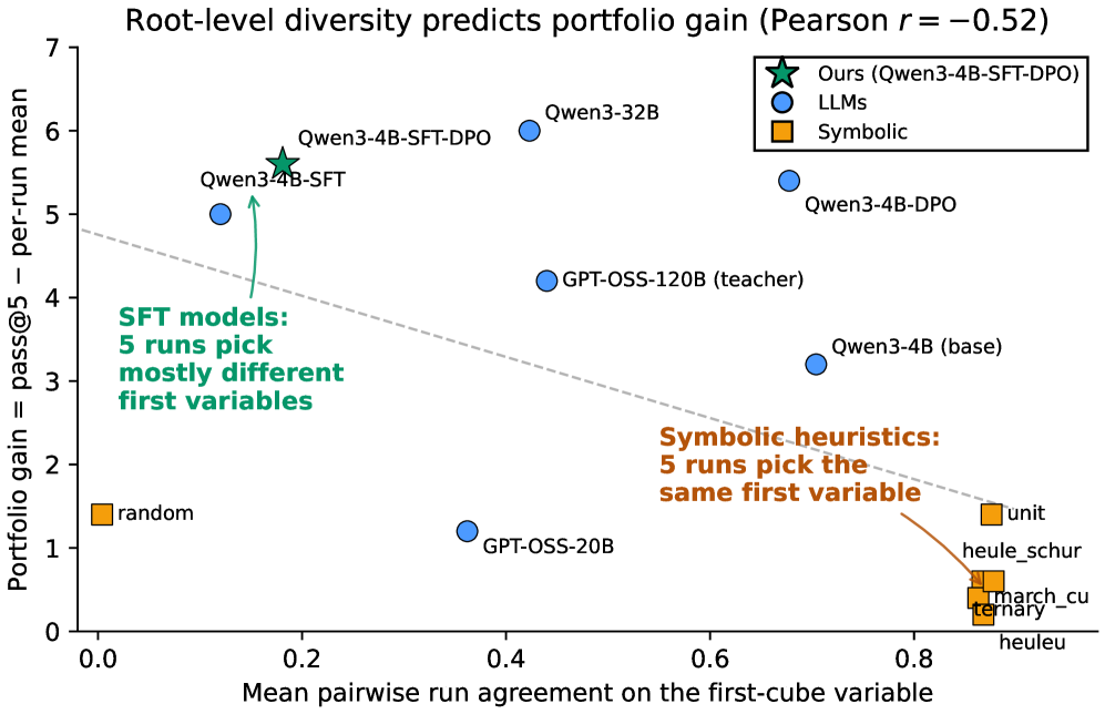
This per-run diversity is not a generic LLM property (Figure˜2). An entropy/agreement ablation on realized first-cube variables across seven baselines (Section˜A.4.2) shows that the untrained Qwen3-4B base and the DPO-only ablation are near-deterministic at the root (mean Shannon entropy 0.55–0.59 bits across 5 runs, 68–70% pairwise run agreement), comparable to deterministic symbolic heuristics (0.22–0.25 bits, 86–88% agreement). SFT lifts the model into a qualitatively different regime: Qwen3-4B-SFT reaches 1.93 bits / 12% agreement, and Qwen3-4B-SFT-DPO retains 1.78 bits / 18% agreement. SFT, not DPO, therefore accounts for the root-level diversity that underlies the 47.4 $\to$ 53 gap; DPO applied on top of SFT trades a small amount of diversity (1.93 $\to$ 1.78 bits) for two additional pass@5 benchmarks (51 $\to$ 53). Across all 13 heuristics (Figure˜2b), first-cube agreement and portfolio gain are negatively correlated (Pearson $r=-0.52$), confirming the diversity-to-coverage link is not specific to our model. Notably, the 4B student exceeds its 120B distillation teacher on all three axes (pass@5: 53 vs 47, entropy: 1.78 vs 1.13 bits, run agreement: 18% vs 44%); full cross-heuristic comparison in Table˜4.

Figure˜7 (in the appendix) shows a fine-grained overview of the heuristic success results. The benchmarks are identified by their index (0-49 SAT, 50-99 UNSAT) and each heuristic is run for five attempts (5 horizontal rows) per benchmark. Green cells indicate a solved benchmark instance, while yellow cells represent failure to solve with a timeout of 30 minutes. Qwen3-4B-SFT-DPO, in pass@5, solves two benchmarks (24, 73) that unit did not, while unit solves two benchmarks (30, 77) that our model could not, a concrete instance of the complementary coverage that motivates a portfolio combination. Table˜1 also reveals SAT/UNSAT performance differences. Paired t-tests (Section˜A.7) show that most heuristics are balanced, with five exceptions: the symbolic unit, heule_schur, and march_cu heuristics all lean SAT ($p=0.033$, $0.025$, $0.003$ respectively), consistent with the SAT split’s concentration on hard random 3-SAT instances (Sections˜A.6 and A.7), a class where lookahead heuristics like these typically outperform CDCL alone; GPT-OSS-120B leans UNSAT (20.8 vs 22.0, $p=0.033$); and Qwen3-4B-DPO (DPO only, no SFT) has a strong UNSAT bias (19.8 vs 21.8, $p=0.003$). Notably, our main model Qwen3-4B-SFT-DPO is well-balanced (SAT=23.8, UNSAT=23.6, $p=0.778$), suggesting that SFT provides a balanced foundation that DPO preserves.

(a) Cumulative distribution of test benchmark CDCL solve times (timeout =24h). 34 problems remained unsolved.

(b) Solved benchmarks weighted and ordered by CDCL solve time [0-49 sat, 50-99 unsat]. Green implies solved benchmark, red is unsolved ($<$30min). Deeper color denotes longer CDCL solve time.

Figure 3: CDCL solve time (without cubing) acts as a proxy for problem difficulty.

(a) Accumulated decision time (sec) per heuristic according to their best attempts. Larger models need more time to decide.

(b) Total cubing decisions made per benchmark (deeper color denotes more decisions). Symbolic heuristics and smaller models make more decisions in allotted time.

Figure 4: Larger models have larger response time, leading them to fewer total decisions than the symbolic heuristics.

To better understand the difficulty distribution of the chosen benchmarks, we measure the time to solve each benchmark with a CDCL solver as a proxy of hardness. Figure˜3(a) displays the cumulative solve time distribution of the test benchmarks, running the glucose v4.2 solver with a timeout of 24h. We see that roughly $58\%$ of our benchmarks could be solved in 1000 sec (16.6 min), while $34\%$ of them could not be solved in 24 hours (top right vertical line). To showcase this difficulty in our experiments, Figure˜3(b) presents the time each C&C run spent for SAT solving (conquering phase). Here, the cell color (green, red) indicates whether the benchmark was solved, while the color hue indicates benchmark difficulty. Deeper green indicates successful but time consuming attempts, while deeper red indicates that C&C timed out. We observe that all heuristics performed similarly on easier (or harder) problems, with a few of the medium-challenging problems acting as the differentiators.

Decision time matters because it bounds how many splits each heuristic can make within the 30-minute timeout. Figure˜4(a) reveals three regimes: large LLMs (Claude-Sonnet-4, GPT-OSS-120B) at the top, the symbolic unit heuristic at the bottom, and our fine-tuned models in the middle alongside the base Qwen3-4B, motivating the choice of a small LLM for end-to-end C&C. Qwen3-4B-SFT-DPO is faster than the base Qwen3-4B despite identical parameter count; inspection of the inference logs attributes this to fewer output-formatting retries. The full per-heuristic graph is in Figure˜8.

Figure˜4(b) shows the same three-tier structure in decision count: the slowest LLMs make the fewest decisions, which combined with their lower pass@5 scores supports the claim that response time hinders exploration. Count, however, does not imply quality, because Claude-Sonnet-4 solves more problems than faster heuristics such as Qwen3-4B.

Learned Heuristic Analysis. A post-hoc LLM-as-judge classification of 388 reasoning traces distributes reasoning patterns across established SAT heuristic categories (Table˜2, left block; full 11-row taxonomy in Table˜6). Variable Frequency Analysis (H1, 73.5%) is dominant, but Section˜A.4.1 shows this frequency preference is shared by every LLM we measured (including the untrained base) and is therefore best read as a calibration observation rather than a training outcome. Two human experts (A and B) independently primary-labelled a random sample of 50 traces; the right block of Table˜2 compares the three raters, and the summary statistics at the bottom (Cohen’s $\kappa$, Fleiss’ $\kappa$) confirm the LLM judge agrees with each human (0.45 and 0.48, moderate) within the range of inter-human disagreement (0.37); the full methodology is in Sections˜A.2 and A.8.4.

Table 2: Left block: top-7 primary heuristics on the full 388-trace classification (Cnt: trace count, %: share of 388, Pri: traces where this was the primary label). Right block: 50-trace inter-rater validation, reporting how Human A, Human B, and Claude-Sonnet-4.5 assigned primary labels; Claude $\kappa$ vs A/B are per-heuristic Cohen’s $\kappa$ against each human. Summary row: overall pairwise $\kappa$ and Fleiss’ $\kappa$ across all three raters. Full 11-row distribution in Table˜6.

			Full (n=388)			Validation (n=50)
ID	Heuristic	Literature	Cnt	%	Pri	A	B	Cl	$\kappa_{A,Cl}$	$\kappa_{B,Cl}$
H1	Variable Frequency	Moskewicz et al. (2001)	285	73.5	192	16	21	24	0.43	0.56
H2	Balanced Splitting	Heule et al. (2011)	170	43.8	60	7	4	6	0.56	0.34
H6	Complexity Reduction	Heule et al. (2011)	169	43.6	37	6	3	9	0.30	0.45
H7	Polarity Balance	Silva and Sakallah (1996)	89	22.9	59	10	12	9	0.81	0.58
H5	Structural Pattern	Ansótegui et al. (2019)	33	8.5	9	4	3	1	$-$0.03	0.48
H4	Clause-Size Weighting	Jeroslow and Wang (1990)	32	8.2	3	0	0	0	—	—
H3	Clause Elimination	Davis et al. (1962)	30	7.7	5	2	3	0	0.00	0.00
Overall   $\kappa_{A,B}=0.37$   $\kappa_{A,Cl}=0.45$   $\kappa_{B,Cl}=0.48$   Fleiss’ $\kappa$ (A + B + Cl) = 0.43

6 Limitations

We note four limitations. Formula size. Context-window constraints restrict us to formulas with up to 600 variables and 1000 clauses; sliding-window attention, formula chunking, or hierarchical variable selection are natural mitigations but remain unexplored. Inference cost. Per-decision inference is slower than CPU-based symbolic heuristics (Figure˜4(a)); our 30-minute-per-benchmark evaluation shows this does not prevent matching the best symbolic heuristic on pass@5, but the gap would widen under tighter budgets. Depth of the mechanism claim. Our mechanism analysis (Figure˜2) examines only the first-cube decision; whether SFT’s diversity effect persists at depth is open. Scope of the benchmarks. Our findings about SFT-driven diversity may not transfer to instance families with very different clause structure (e.g., random 3-SAT at the phase transition).

7 Conclusion

We presented the first successful approach for training transformers to learn effective cubing heuristics for Cube-and-Conquer SAT solving. Our neuro-symbolic post-training framework enables a 4B-parameter model to achieve pass@5 of 53, matching the best symbolic heuristics and surpassing frontier LLMs. Ablations show clear progression: SFT improves the base model from 46 to 51, while adding DPO reaches 53, demonstrating that transformers can acquire effective cubing policies with appropriate supervision. An ablation on realized first-cube decisions further identifies SFT, rather than DPO, as the training stage responsible for root-level decision diversity, with DPO contributing two additional pass@5 benchmarks on top. Unlike the symbolic heuristics it matches on pass@5, which all lean significantly toward SAT instances, our model is SAT/UNSAT-balanced and solves complementary benchmarks, making it a candidate for portfolio-based solvers. The same framework could apply to other NP-hard decision problems whose solvers rely on learned branching heuristics, such as QBF (Zhang and Malik, 2002; Biere et al., 2009) and SMT (De Moura and Bjørner, 2008).

Appendix A Appendix

Figure 5: Solved benchmarks weighted and ordered by CDCL solve time [sat,unsat]. Green implies solved benchmark, red is unsolved ($<30min$). Deeper color denotes longer CDCL solve time.

Figure 6: Total decisions made per benchmark (green implies fewer decisions). Symbolic heuristics and smaller models make more decisions in allotted time.

Figure 7: Fine-grained overview of successes (green) and unknowns (yellow) for each benchmark. First 50 benchmarks are SAT, last 50 are UNSAT. The heuristics are sorted based on pass@5 score.

Figure 8: Accumulated decision time (sec) per heuristic according to their best attempts. Larger models need more time to decide and respond.

Figure 9: Neuro-symbolic post-training pipeline. A teacher model first creates SFT data for the first training stage. Monte-Carlo-Tree Search is then guided by symbolic cubing decisions to create DPO data, which is augmented with reasoning traces from the teacher model.

A.1 Training Hyperparameters

Table˜3 reports the full set of training hyperparameters used to produce the three model variants (Qwen3-4B-DPO, Qwen3-4B-SFT, Qwen3-4B-SFT-DPO) discussed in Section˜5. The end-to-end neuro-symbolic post-training pipeline that generates the SFT and DPO data is illustrated in Figure˜9.

Table 3: Training Hyperparameters

Model Name	Qwen3-4B-DPO	Qwen3-4B-SFT	Qwen3-4B-SFT-DPO
Max Length	8192	17500	8192
Max Prompt Length	6144	-	6144
Per Device Train Batch Size	1	1	1
Per Device Eval Batch Size	8	-	8
Gradient Accumulation Steps	8	32	8
Number of Epochs	2	2	3
Learning Rate	5e-6	1e-5	5e-6
Optimizer	adamw_8bit	adamw_torch_fused	adamw_8bit
Weight Decay	0.1	0.01	0.1
Learning Rate Scheduler	cosine	cosine	cosine
Warmup Ratio	0.1	0.05	0.1
GPUs	8 H100-80G	8 H100-80G	8 H100-80G
Duration	3h 10m 11s	1h 6m 18s	8h 50m 30s
Checkpoint	final	final	150 global step

A.2 Inter-Rater Agreement for Heuristic Classification

To validate the LLM-as-a-judge approach, two human experts (A and B) independently classified the same random sample of 50 reasoning traces into the primary-heuristic categories. We then ran the same classification prompt via Claude-Sonnet-4.5 and computed Cohen’s $\kappa$ [Cohen, 1960] on the primary label and Fleiss’ $\kappa$ across all three raters. Per-heuristic counts and Claude-vs-human $\kappa$ for the top-7 categories are reported in the right block of Table˜2 in the main body; the overall pairwise $\kappa$ is 0.45 (Human A vs Claude) and 0.48 (Human B vs Claude), both in the moderate Landis–Koch range, and slightly above inter-human agreement (0.37) on the same 50 traces. Fleiss’ $\kappa$ = 0.43 across all three raters confirms the LLM judge performs within the range of human-to-human disagreement. Per-heuristic $\kappa$ is cleanest on Polarity Balance (H7) and H1 Variable Frequency. The near-zero or negative per-heuristic $\kappa$ for H3 and H5 reflects very low base rates (at most 4 primaries out of 50 on either rater’s sheet), where $\kappa$ is numerically unstable; the raw counts remain close across raters.

A.3 Theoretical Analysis of the Learning Framework

We provide a formal mathematical analysis of our neuro-symbolic training framework, including the MDP formulation, reward function properties, and training objectives.

A.3.1 MDP Formulation for Cubing

We formalize the cubing problem as a Markov Decision Process (MDP) $\mathcal{M}=(\mathcal{S},\mathcal{A},T,R,\gamma)$ [Russell et al., 1995]:

State Space $\mathcal{S}$: The set of all CNF formulas $\phi$ that can arise during cube-and-conquer. Each state $s\in\mathcal{S}$ represents a CNF formula after zero or more splitting decisions have been applied.

Action Space $\mathcal{A}(s)$: For a state $s$ representing formula $\phi$, the action space is $\mathcal{A}(s)=\text{Vars}(\phi)$, the set of unassigned variables in $\phi$. Selecting action $v$ corresponds to choosing variable $v$ as the splitting variable.

Transition Function $T$: The transition is deterministic. Given state $s$ (formula $\phi$) and action $v$, the transition produces two child states:

$$T(s,v)=\left(\text{simplify}(\phi\land v),\text{simplify}(\phi\land\neg v)\right)$$ (4)

where $\text{simplify}(\cdot)$ applies unit propagation and clause elimination.

Reward Function $R$: As defined in Equation˜2, the reward captures the quality of a splitting decision.

Discount Factor $\gamma$: In our formulation, we use $\gamma=1$ (undiscounted) since we care about total solving efficiency.

The optimal policy $\pi^{*}$ satisfies the Bellman optimality equation:

$$~V^{*}(s)=\max_{v\in\mathcal{A}(s)}\left[R(s,v)+\frac{1}{2}\left(V^{*}(s_{v}^{+})+V^{*}(s_{v}^{-})\right)\right]$$ (5)

where $s_{v}^{+}=\text{simplify}(\phi\land v)$ and $s_{v}^{-}=\text{simplify}(\phi\land\neg v)$ are the two child states. The factor of $\frac{1}{2}$ reflects that both branches must be solved in cube-and-conquer.

A.3.2 Reward Function Analysis

We analyze the mathematical properties of our reward function from Equation˜2:

$$R_{\text{node}}=\frac{\log(1+\varepsilon+u+e)}{\log(1+\varepsilon+u+e+d+c)}$$ (6)

where $\varepsilon>0$ is a small constant ensuring numerical stability by preventing $\log(1)=0$ in degenerate cases where all metrics are zero.

Proposition A.1 (Boundedness).

For all non-negative values $u,e,d,c\geq 0$ and $\varepsilon>0$, we have $R_{\text{node}}\in(0,1]$.

Proof.

Let $N=1+\varepsilon+u+e$ (numerator argument) and $D=1+\varepsilon+u+e+d+c$ (denominator argument).

Upper bound: Since $d,c\geq 0$, we have $D\geq N>1$. Therefore $\log(D)\geq\log(N)>0$, which implies $R=\frac{\log(N)}{\log(D)}\leq 1$ with equality when $d=c=0$.

Lower bound: Since $N\geq 1+\varepsilon>1$ and the logarithm is positive for arguments greater than 1, both numerator and denominator are positive. Thus $R>0$. ∎

Proposition A.2 (Monotonicity).

The reward function $R$ is (1) monotonically increasing in $u$ and $e$ (unit propagations and eliminated clauses), and (2) monotonically decreasing in $d$ and $c$ (decisions and conflicts).

Proof.

Let $N=1+\varepsilon+u+e$ and $D=N+d+c$. Then $R=\frac{\log N}{\log D}$.

Increasing in $u$ (and similarly $e$): $\frac{\partial R}{\partial u}=\frac{D\cdot\log D-N\cdot\log N}{N\cdot D\cdot\log^{2}D}$.

We have $D\geq N>1$, so $\log^{2}D>0$, thus we need to show $D\cdot\log D-N\cdot\log N\geq 0\implies D\cdot\log D\geq N\cdot\log N$.

So, $D\geq N>1\implies\log D\geq\log N>0$, thus $D\cdot\log D\geq N\cdot\log N$, thus $D\cdot\log D\>\geq N\cdot\log N$.

Decreasing in $d$ (and similarly $c$): $\frac{\partial R}{\partial d}=-\frac{\log N}{D\cdot\log^{2}D}<0$ since $\log N>0$, $D\geq N>1$, and $\log D\geq\log N>0$. ∎

Proposition A.3 (Limiting Behavior).

(1) When $d=c=0$ (immediately solved formula): $R=1$. (2) As $d+c\to\infty$ (very hard formula): $R\to 0$.

Proof.

Case 1: When $d=c=0$, we have $D=N$, so $R=\frac{\log N}{\log N}=1$. Case 2: As $d+c\to\infty$, $D\to\infty$ while $N$ remains fixed. Thus $\lim_{D\to\infty}\frac{\log N}{\log D}=0$. ∎

A.3.3 DPO Training Objective

Direct Preference Optimization (DPO) [Rafailov et al., 2023] learns from preference pairs without explicit reward modeling. Given a dataset $\mathcal{D}=\{(x_{i},y_{w}^{i},y_{l}^{i})\}$ where $y_{w}$ is preferred over $y_{l}$ for prompt $x$, the DPO loss is:

$$~\mathcal{L}_{\text{DPO}}(\pi_{\theta};\pi_{\text{ref}})=-\mathbb{E}_{(x,y_{w},y_{l})\sim\mathcal{D}}\left[\log\sigma\left(\beta\cdot h_{\theta}(x,y_{w},y_{l})\right)\right]$$ (7)

where $\sigma$ is the sigmoid function, $\beta$ is a temperature parameter, and:

$$h_{\theta}(x,y_{w},y_{l})=\log\frac{\pi_{\theta}(y_{w}|x)}{\pi_{\text{ref}}(y_{w}|x)}-\log\frac{\pi_{\theta}(y_{l}|x)}{\pi_{\text{ref}}(y_{l}|x)}$$ (8)

The key insight of DPO is that it implicitly optimizes an equivalent objective to RLHF under the Bradley-Terry preference model. Specifically, DPO learns a policy $\pi_{\theta}$ such that the implicit reward $r^{*}(x,y)=\beta\log\frac{\pi_{\theta}(y|x)}{\pi_{\text{ref}}(y|x)}$ satisfies $r^{*}(x,y_{w})>r^{*}(x,y_{l})$ for preferred responses.

Connection to Cubing.

In our setting, $x$ is the CNF formula (prompt), $y$ is the reasoning trace and cube decision, and preference $y_{w}\succ y_{l}$ is determined by our cube scoring function (Equation˜3).

A.3.4 Cube Scoring Function Analysis

Our cube scoring function from Equation˜3 combines rewards from both branches:

$$\text{score}(l,\neg l)=\underbrace{R_{l}\cdot R_{\neg l}}_{\text{balance term}}+\underbrace{R_{l}+R_{\neg l}}_{\text{progress term}}$$ (9)

Proposition A.4 (Symmetry).

The scoring function is symmetric: $\text{score}(l,\neg l)=\text{score}(\neg l,l)$.

Proof.

Both the product $R_{l}\cdot R_{\neg l}$ and sum $R_{l}+R_{\neg l}$ are symmetric in their arguments. ∎

Proposition A.5 (Balance Incentive).

For fixed total progress $R_{l}+R_{\neg l}=S$, the score is maximized when $R_{l}=R_{\neg l}=S/2$ (balanced branches).

Proof.

Given constraint $R_{l}+R_{\neg l}=S$, let $R_{l}=t$ and $R_{\neg l}=S-t$. The score becomes $f(t)=t(S-t)+S=-t^{2}+St+S$. Taking the derivative: $f^{\prime}(t)=-2t+S=0\implies t=S/2$. The second derivative $f^{\prime\prime}(t)=-2<0$ confirms this is a maximum. ∎

Proposition A.6 (Score Range).

For rewards $R_{l},R_{\neg l}\in(0,1]$, the score satisfies $\text{score}(l,\neg l)\in(0,3]$ with maximum achieved when $R_{l}=R_{\neg l}=1$.

Proof.

Upper bound: When $R_{l}=R_{\neg l}=1$: $\text{score}=1\cdot 1+1+1=3$. Lower bound: As $R_{l},R_{\neg l}\to 0^{+}$, both terms approach 0, so $\text{score}\to 0^{+}$. ∎

A.3.5 Comparison with Alternative Reward Designs

We considered several alternative reward formulations:

Additive Reward.

$R_{\text{add}}=\alpha(u+e)-\beta(d+c)$. This linear formulation lacks boundedness and can produce unbounded negative rewards, destabilizing training.

Multiplicative Reward.

$R_{\text{mult}}=\frac{u+e+1}{d+c+1}$. While bounded below by 0, this can grow unboundedly large (depending on the formula’s number of clauses) when $d=c=0$ but $u,e$ are large.

Time-Based Reward.

$R_{\text{time}}=\frac{1}{1+t_{\text{solve}}}$. Directly using solve time $t_{\text{solve}}$ introduces high variance due to system noise, caching effects, and non-determinism in parallel solvers.

Our log-ratio formulation (Equation˜2) combines the benefits of boundedness, stability, and monotonicity while avoiding the drawbacks of these alternatives.

A.4 Quantitative Analysis of Decision Behaviour

The heuristic classification in Table˜6 summarises what the model says it is doing, based on a post-hoc LLM-judge reading of the reasoning text. In this section we examine what the model actually does, by parsing the DIMACS prompt of each cubing decision and comparing the chosen variable against structural properties of the formula. All analyses focus on the first-cube (root) decision, the only decision point where every heuristic faces an identical formula across models, and use the 100 test benchmarks (50 SAT, 50 UNSAT) across 5 evaluation runs. In addition to our main model, we include baselines from every heuristic reported in Table˜1: the Qwen3-4B base model, the SFT-only and DPO-only ablations, two teacher candidates (GPT-OSS-20B, GPT-OSS-120B), a larger LLM baseline (Qwen3-32B), and six symbolic heuristics (unit, heule_schur, march_cu, heuleu, ternary, random).

A.4.1 Do the chosen variables match the dominant heuristic (H1)?

We count the clause-occurrence frequency of every variable in each CNF and rank the chosen first-cube variable by that count. A rank percentile of 0 means the chosen variable is the most frequent in the formula; 0.5 is the median; a uniformly-random selector over the variable index space would have mean 0.5.

Figure˜10 shows the distribution for Qwen3-4B-SFT-DPO alone. 91% of SAT first-cube choices and 73% of UNSAT first-cube choices lie in the top 10% most-frequent variables (median rank percentile 0.000 and 0.004 respectively; overall mean 0.08). Taken in isolation, this number appears to confirm the H1 (Variable Frequency Analysis) majority in Table˜6 at the level of realised decisions. However, the same measurement on the baselines and symbolic heuristics (Table˜4) reveals that the top-10% behaviour is essentially universal across LLMs: the untrained Qwen3-4B base sits at 79%, the GPT-OSS-120B teacher at 90%, and even random reaches 74% because clause-occurrence frequency is heavy-tailed and hitting the top 10% is geometrically common. Symbolic lookahead heuristics explicitly designed around clause weighting (unit, heule_schur, march_cu, etc.) cluster at 85–86%. We therefore read this metric as a calibration result: all LLMs we measured and our trained model in particular operate well inside the same “top-frequency tail” as established symbolic heuristics, rather than as evidence of a behaviour that post-training introduced.

Figure 10: Clause-occurrence rank percentile of the first-cube variable chosen by Qwen3-4B-SFT-DPO, pooled over 5 runs $\times$ 100 benchmarks (250 SAT + 250 UNSAT decisions). Left: histogram. Right: cumulative distribution versus a uniform-random baseline. 91% of SAT and 73% of UNSAT choices lie in the top 10% of variables by clause frequency. Table˜4 shows that this behaviour is largely shared by other LLMs and by symbolic baselines.

A.4.2 Where does solution diversity come from? A cross-heuristic comparison

Table˜9 shows that Qwen3-4B-SFT-DPO solves 53 unique benchmarks across 5 runs while averaging 47.4 per run—the gap is evidence that different runs solve different benchmarks. We quantify the diversity that produces this gap by (i) measuring the Shannon entropy of the first-cube variable across the 5 runs per benchmark (upper bound $\log_{2}5\approx 2.32$ bits), and (ii) computing the mean pairwise run agreement—the fraction of benchmarks on which two different runs pick the same first-cube variable. All LLMs in this comparison share an identical inference configuration (same temperature and top-$p$ settings on the same vLLM server), so any diversity differences between models reflect training, not decoding-time sampling. Contrasting our model against the same set of baselines used in Section˜A.4.1 isolates which training stage unlocks diversity.

Table˜4 reports both axes for every heuristic, and Figure˜2 in the main body plots them together. Three clear regimes emerge:

Symbolic heuristics (unit, heule_schur, march_cu, heuleu, ternary) cluster tightly at mean entropy 0.23–0.25 bits and run agreement 86–88%. Apart from tie-breaking, these heuristics are deterministic, which bounds how much portfolio benefit any repeated run can extract from them. random sits at the opposite extreme (entropy 2.31, agreement 0%).

Base and DPO-only LLMs behave almost symbolically: the untrained Qwen3-4B has entropy 0.55 and agreement 70%, and the DPO-only ablation (Qwen3-4B-DPO) is nearly identical at 0.59 / 68%. These models are near-deterministic at the root in the sense that their temperature-sampled decodes usually resolve to the same first cube across runs.

SFT-based LLMs are genuinely diverse. Qwen3-4B-SFT and Qwen3-4B-SFT-DPO reach entropy 1.93 and 1.78 with run agreement 12% and 18% respectively—more diverse than either the 20B teacher candidate (1.29 / 36%), the 120B teacher (1.13 / 44%), or the 32B baseline (1.17 / 42%). DPO after SFT slightly narrows the diversity (1.93 $\rightarrow$ 1.78) without collapsing it; this is consistent with the DPO objective concentrating probability on high-reward variables while still leaving meaningful mass on alternatives.

Because base-only and DPO-only ablations share the base model’s near-deterministic root behaviour, SFT is the training stage that produces the diversity observed in our main model. This gives a specific mechanistic interpretation for why Qwen3-4B-SFT-DPO contributes complementary coverage in a portfolio setting while symbolic heuristics cannot: the symbolic heuristics’ agreement ceiling of 86–88% means five independent runs mostly re-solve the same benchmarks, whereas our model’s 18% agreement spreads five runs over largely disjoint first moves.

Figure˜11 tests the connection between root-level diversity and portfolio gain directly. For each heuristic in Table˜1, we plot its mean pairwise run agreement against its portfolio gain, defined as the difference between pass@5 (the union of benchmarks solved across 5 runs) and the per-run mean (the average number of benchmarks solved in a single run). Portfolio gain measures the extra benchmarks that a 5-run portfolio recovers over a single run: for example, Qwen3-4B-SFT-DPO solves 47.4 benchmarks per run on average but 53 unique benchmarks across 5 runs, for a gain of $+5.6$; the symbolic unit heuristic solves 51.6 per run and 53 across 5 runs, for a gain of only $+1.4$. Both reach the same pass@5, but through different mechanisms: unit by solving a strong, stable set every run, and Qwen3-4B-SFT-DPO by solving different, complementary sets across runs. The relationship is negative (Pearson $r=-0.52$ across 13 heuristics): heuristics with lower root-level agreement tend to extract more benefit from additional attempts. This supports the claim that the root-level diversity produced by SFT is what translates into the complementary per-run coverage observed in the main body.

Figure 11: Root-level decision diversity versus portfolio gain, one point per heuristic in Table˜1. Horizontal: mean pairwise run agreement on the first-cube variable (0 = every pair of runs picks a different variable, 1 = every pair picks the same variable). Vertical: pass@5 $-$ per-run mean, i.e. the extra benchmarks a 5-run portfolio recovers over a single run. Heuristics with lower agreement tend to gain more from repeated attempts (Pearson $r=-0.52$). Symbolic heuristics cluster in the deterministic / low-gain corner (5 runs re-solve the same set); SFT-based LLMs occupy the diverse / high-gain corner (5 runs solve different, complementary sets).

Table 4: First-cube measurements for every heuristic reported in Table˜1. Top 10% and Top 25%: fraction of first-cube choices whose chosen variable is within the top 10% and top 25% of the CNF’s variables by clause-occurrence frequency. Entropy: mean Shannon entropy of the first-cube variable across 5 runs per benchmark (max attainable $\log_{2}5\approx 2.32$). Agreement: mean pairwise run agreement on the first-cube variable. All rows pool 5 runs over the 100 test benchmarks. (The median rank percentile is 0.000 for all methods.)

Family	Heuristic / Model	Top 10%	Top 25%	Entropy	Agreement
LLM	Qwen3-4B (base)	79.0%	87.4%	0.55	70.4%
LLM	Qwen3-4B-SFT	79.8%	86.0%	1.93	12.0%
LLM	Qwen3-4B-DPO	81.7%	89.8%	0.59	67.8%
LLM	Qwen3-4B-SFT-DPO	78.8%	85.0%	1.78	18.1%
LLM	GPT-OSS-20B	84.0%	89.4%	1.29	36.2%
LLM	GPT-OSS-120B (teacher)	89.8%	93.8%	1.13	44.0%
LLM	Qwen3-32B	88.6%	91.6%	1.17	42.3%
Symbolic	unit	85.6%	87.8%	0.23	87.6%
Symbolic	heule_schur	85.4%	88.0%	0.24	86.7%
Symbolic	march_cu	85.0%	87.2%	0.25	86.3%
Symbolic	heuleu	85.2%	87.4%	0.24	86.8%
Symbolic	ternary	85.4%	88.0%	0.22	87.8%
Symbolic	random	73.6%	80.4%	2.31	0.4%

Per-benchmark diversity view.

Figure˜12 complements the cross-heuristic comparison with a per-benchmark view restricted to Qwen3-4B-SFT-DPO. On half of the 100 benchmarks the most-popular first-cube variable is picked by only 1 of 5 runs; 27 benchmarks have a 2/5 mode, 18 have a 3/5 mode, 5 have a 4/5 mode, and no benchmark has 5/5 agreement.

Figure 12: Per-benchmark diversity of the first-cube variable chosen by Qwen3-4B-SFT-DPO across 5 evaluation runs. Left: positional bias, i.e. the distribution of chosen variable index divided by the total number of variables in the formula. Middle: how often the most-common first-cube variable dominates the 5 runs: on 50/100 benchmarks the top choice wins only 1 of 5 runs; no benchmark has 5/5 agreement. Right: pairwise run-agreement matrix (student only)—all off-diagonal entries are 8–20%, agreeing with the mean 18% reported in Table˜4.

A.4.3 Is the H1–H12 classification confounded with decoding style?

The H1–H12 labels in Table˜6 are assigned from reasoning text using an LLM-as-a-judge. To test whether these labels reflect genuine reasoning differences or are an artifact of decoding variability, we ran an unsupervised clustering on 2000 reasoning traces (400 from each of the 5 evaluation runs, balanced over SAT and UNSAT, numerical tokens masked to prevent benchmark-specific leakage). TF-IDF features (unigrams and bigrams) were reduced to 50 dimensions via truncated SVD and clustered with $k$-means for $k\in\{3,\ldots,10\}$, selecting the best $k$ by silhouette score.

The best silhouette score, 0.189 at $k=9$, is weak (silhouette $>0.5$ typically indicates well-separated clusters). More importantly, the clusters that do emerge (Figure˜13, Table˜5) align almost perfectly with the run identity rather than with heuristic categories: for example, one 399-trace cluster is 100% from Run 5 (distinguishing vocabulary: “propagation”, “unit”, “activity”, “neighbor”), another 397-trace cluster is 99.7% from Run 4 (“simplified”, “balanced”, “structural properties”), and a 399-trace cluster is 100% from Run 2 (“solve”, “input”, “num true”). Each decoding seed produces its own characteristic surface vocabulary.

This finding tempers the interpretation of Table˜6: the H1–H12 categories capture strategies invoked in the reasoning text, but per-trace lexical style is driven as much by decoding variance as by underlying decision policy. Because our main behavioural claim (Section˜A.4.2) rests on realised first-cube variables rather than on reasoning text, it is unaffected by this confound.

Figure 13: Unsupervised clustering of 2000 reasoning traces (400 per run, SAT/UNSAT balanced, numerical tokens masked). TF-IDF features reduced via truncated SVD, $k$-means with $k{=}9$ chosen by silhouette (score 0.19). 2D t-SNE projection coloured by cluster. Table˜5 lists the per-cluster distinguishing terms.

Table 5: Per-cluster size, dominant decoding run, and top eight distinguishing terms (relative to the global mean) for the unsupervised clustering in Figure˜13. The dominant run accounts for 94–100% of every cluster, indicating that surface vocabulary tracks decoding seed more than reasoning strategy.

C	n	Dom.	Top distinguishing terms
		run	(vs. global mean)
C4	402	Run 2	solve, input, num true, cnf input, variable negation, resulting, resulting subformulas, pair
C0	399	Run 5	propagation, unit, activity, neighbor, unit propagation, neighbor activity, potential, short
C1	398	Run 4	simplified, difficulty, structural, properties, balanced simplified, balanced, structural properties, impact
C3	323	Run 1	frequent variable, appears clauses, simplifies, clauses fixing, fixing, fixing true, assigning true, easiest subformulas
C2	138	Run 3	negative num, positive num, num total, num positive, num negative, total clauses, total, num variable
C5	132	Run 3	positive num, num negative, satisfies num, satisfies, appears num, num positive, reduction, negative num
C8	95	Run 1	high clause, variables high, high, clause frequency, likely, clause frequencies, clause counts, likely split
C7	67	Run 3	occurrences num, positive occurrences, total clauses, negative occurrences, num percentage, num total, percentage, total
C6	46	Run 3	neg, pos, num pos, neg num, pos num, num neg, num freq, freq num

A.5 Learned Heuristic Classification of Reasoning Traces

To understand what strategies our model invokes in its reasoning text, we analyzed 388 output traces (191 SAT, 197 UNSAT) produced by Qwen3-4B-SFT-DPO and classified them into established SAT heuristic categories. An LLM-as-a-judge (Claude-Sonnet-4.5) parsed each trace, which typically contains 1–3 sentences of reasoning followed by a variable decision. The classifier prompt (Section˜A.8.4) includes an explicit primary-heuristic selection rule and five worked few-shot examples drawn from traces where two independent human annotators agreed on the primary label. Since traces often exhibit multiple heuristics, the classifier assigns all applicable categories plus a primary label. To validate this automated classification, two human experts independently labeled a random sample of 50 traces; the LLM judge’s Cohen’s $\kappa$ with each human (0.45 and 0.48) lands in the moderate-agreement range and is slightly above inter-human agreement itself (0.37), indicating that the LLM judge performs within the range of human disagreement (Section˜A.2).

Table 6: Heuristic Classification of (388) Reasoning Traces of Qwen3-4B-SFT-DPO

ID	Heuristic	Count	%	Primary	Literature
H1	Variable Frequency Analysis	285	73.5	192	Moskewicz et al. [2001]
H2	Balanced Subformula Splitting	170	43.8	60	Heule et al. [2011]
H6	Subformula Complexity Reduction	169	43.6	37	Heule et al. [2011]
H7	Polarity Balance Analysis	89	22.9	59	Silva and Sakallah [1996]
H5	Structural Pattern Recognition	33	8.5	9	Ansótegui et al. [2019]
H4	Clause-Size Weighting	32	8.2	3	Jeroslow and Wang [1990]
H3	Clause Elimination Reasoning	30	7.7	5	Davis et al. [1962]
H8	Critical Clause Identification	20	5.2	7	Freeman [1995]
H12	Other	14	3.6	11	—
H9	Unit Propagation Potential	9	2.3	5	Le Berre [2001]
H10	Symmetry Detection	4	1.0	0	Katebi et al. [2010]

The dominant heuristic is Variable Frequency Analysis (H1, 73.5% of traces, primary in 192 of 388), which counts variable occurrences across clauses. The next most frequent are Balanced Subformula Splitting (H2, 43.8%) and Subformula Complexity Reduction (H6, 43.6%), followed by Polarity Balance (H7, 22.9%). The remaining heuristics are less frequent ($<9\%$); concrete examples for each are in Section˜A.9. This classification shows that the model’s reasoning text invokes a diverse set of established SAT heuristics, with H1 being the default strategy without being explicitly prompted. Sections˜A.4.1 and A.4.3 provide two caveats on the interpretation of these counts: the H1 top-frequency behavior is shared by every LLM we measured (not training-specific), and unsupervised clustering of the reasoning text shows that per-trace surface vocabulary partly reflects decoding seed rather than reasoning strategy.

A.6 Benchmark Family Distribution

Table˜7 reports the per-family breakdown of the 100 test benchmarks classified by SAT-Competition naming convention. Families were inferred from the Global Benchmark Database filename prefix; the classification script is released with the code. The distribution is weighted toward hard random 3-SAT (34%, mostly sgen) and XOR / modular-arithmetic (19%), the instance classes for which Cube-and-Conquer was originally developed [Heule et al., 2011]. The SAT split is more concentrated ($28/50$ sgen + 6 Barthel + 3 random-graph = 74% hard-random) than the UNSAT split, which spans ten families without any dominating above 18%.

Table 7: Per-family distribution of the 100 test benchmarks, inferred from SAT-Competition filename prefixes.

Family	SAT	UNSAT	Total
Hard random 3-SAT (sgen / hgen)	28	6	34
XOR / modular-arithmetic	11	8	19
Graph encodings (edges / fixedbandwidth / random graphs)	3	9	12
Urquhart (constraint graph)	1	9	10
Combinatorial puzzles (pigeonhole / battleship)	1	5	6
Frustrated-loops (Barthel / glassy)	6	0	6
Cryptographic (Hidden Weighted Bit)	0	5	5
Margulis (expander graph)	0	4	4
ISCAS-like circuit	0	3	3
Model-counting derived	0	1	1
Total	50	50	100

A.7 SAT vs UNSAT Performance Analysis

To investigate whether heuristics exhibit bias toward SAT or UNSAT instances, we perform paired t-tests comparing each heuristic’s SAT performance (out of 50) versus UNSAT performance (out of 50) across 5 runs. Table˜8 reports the results.

Table 8: Paired t-test: SAT vs UNSAT performance per heuristic (5 runs). Significant results ($p<0.05$) are bolded.

Heuristic	SAT avg	UNSAT avg	Diff	$p$-value	Bias
Qwen3-4B	21.2	21.6	$-0.4$	0.689
GPT-OSS-120B	20.8	22.0	$-1.2$	0.033	UNSAT
Claude-3.7-Sonnet	22.0	22.6	$-0.6$	0.426
Qwen3-32B	21.0	22.0	$-1.0$	0.089
Claude-Sonnet-4	23.8	23.0	$+0.8$	0.294
random	22.6	23.0	$-0.4$	0.717
heule_schur	26.4	25.0	$+1.4$	0.025	SAT
march_cu	26.6	25.0	$+1.6$	0.003	SAT
unit	26.4	25.2	$+1.2$	0.033	SAT
Qwen3-4B-DPO	19.8	21.8	$-2.0$	0.003	UNSAT
Qwen3-4B-SFT	22.6	23.4	$-0.8$	0.242
Qwen3-4B-SFT-DPO	23.8	23.6	$+0.2$	0.778

Most heuristics show no significant difference between SAT and UNSAT performance (overall pooled: SAT avg=22.4, UNSAT avg=22.8, $p=0.236$). Five exceptions emerge: (1) unit (symbolic) performs significantly better on SAT instances (26.4 vs 25.2, $p=0.033$); (2) heule_schur (symbolic) also leans SAT (26.4 vs 25.0, $p=0.025$); (3) march_cu (symbolic) leans SAT most strongly (26.6 vs 25.0, $p=0.003$), suggesting the symbolic scoring functions are optimized for satisfiable formula structure; (4) GPT-OSS-120B shows a slight UNSAT bias (20.8 vs 22.0, $p=0.033$); and (5) Qwen3-4B-DPO (DPO only, no SFT) has a strong UNSAT bias (19.8 vs 21.8, $p=0.003$). Notably, our main model Qwen3-4B-SFT-DPO is well-balanced (SAT=23.8, UNSAT=23.6, $p=0.778$), suggesting that the combination of SFT and DPO produces a heuristic without systematic category bias. The SAT bias of the three symbolic lookahead heuristics is consistent with the test-set composition reported in Table˜7: the SAT split is 74% hard random 3-SAT variants (sgen, Barthel, random-graph), a class where lookahead heuristics like these typically outperform CDCL alone.

A.8 Prompts Used

Note that in the following prompts we use the term cube to mean the decision variable as well, inspired by the Z3’s documentation [De Moura and Bjørner, 2008].

A.8.1 System Prompt

We use the following system prompt for the interaction with the different models. The model is expected to respond using two sections: a reasoning section containing analysis, and an answer section with a well-formatted cube. The answer is a parenthesized pair of two opposite integers. For example, the answer $(-1,1)$ indicates that the splitting variable is $1$, so the subformulas are derived by substituting the variable $1$ as True and False.

A.8.2 Task Prompt

The following prompt accompanies each CNF formula input:

A.8.3 DPO Reasoning Generation Prompt

For generating reasoning trajectories in our DPO training data, we use the following prompt with the teacher model:

A.8.4 Heuristic Classification Prompt

For classifying the obtained reasoning traces, we use the following prompt:

A.9 Reasoning Traces and Heuristic Classification Examples

We present five example reasoning traces generated by our trained model (Qwen3-4B-SFT-DPO) during the cubing phase, alongside their classification from Claude-Sonnet-4. These traces contain all of the heuristic categories and have diverse quality (from high to low) according to Claude-Sonnet-4. The mapping of heuristics to examples is: H1 (ex. 2, 3), H2 (ex. 1, 2), H3 (ex. 3), H4 (ex. 4), H5 (ex. 1), H6 (ex. 2), H7 (ex. 3), H8 (ex. 2), H9 (ex. 4), H10 (ex. 1), H12 (ex. 5).

Table 9: Success statistics of different heuristics over 5 attempts on SAT and UNSAT benchmarks, sorted by average total rate. $\sigma$ denotes standard deviation across runs.

		SAT / 50					UNSAT / 50					Total / 100
	Heuristic	1	2	3	4	5	1	2	3	4	5	1	2	3	4	5	Avg	$\boldsymbol{\sigma}$
LLMs	Qwen3-4B	19	24	20	22	21	21	21	22	22	22	40	45	42	44	43	42.8	1.9
	GPT-OSS-120B	21	21	20	20	22	22	22	22	22	22	43	43	42	42	44	42.8	0.8
	Qwen3-32B	23	21	19	22	20	23	23	21	22	21	46	44	40	44	41	43.0	2.4
	GPT-OSS-20B	21	21	23	21	23	22	22	22	22	22	43	43	45	43	45	43.8	1.1
	Claude-3.7-Sonnet	23	22	22	21	22	21	23	23	23	23	44	45	45	44	45	44.6	0.5
	Claude-Sonnet-4	24	26	23	22	24	23	23	23	23	23	47	49	46	45	47	46.8	1.5
Symbolic	random	20	22	24	23	24	24	23	23	23	22	44	45	47	46	46	45.6	1.1
	ternary	26	26	27	26	27	25	25	25	25	25	51	51	52	51	52	51.4	0.5
	heule_schur	25	27	27	26	27	25	25	25	25	25	50	52	52	51	52	51.4	0.9
	unit	26	26	27	26	27	26	25	25	25	25	52	51	52	51	52	51.6	0.5
	march_cu	26	27	26	27	27	25	25	25	25	25	51	52	51	52	52	51.6	0.5
	heuleu	27	27	27	27	26	25	25	25	25	25	52	52	52	52	51	51.8	0.4
Ours	Qwen3-4B-DPO	20	20	19	20	20	22	21	21	23	22	42	41	40	43	42	41.6	1.1
	Qwen3-4B-SFT	25	22	21	24	21	24	23	23	24	23	49	45	44	48	44	46.0	2.3
	Qwen3-4B-SFT-DPO	23	25	24	23	24	23	23	23	25	24	46	48	47	48	48	47.4	0.9

A.10 Symbolic Heuristic Definitions

We compare our learned heuristics against several symbolic lookahead heuristics implemented in Z3 [De Moura and Bjørner, 2008]. These heuristics determine which literal to select for cubing by computing reward scores based on different structural properties of the formula.

A.10.1 Ternary

The ternary heuristic is a reward function optimized for random 3-SAT instances, originally used by Heule and Knuth in the March solver. It focuses on the structure of ternary (3-literal) clauses to guide splitting decisions.

A.10.2 Heule-Schur

The heule_schur heuristic is based on the “Schur Number 5” work by Heule (AAAI 2018), a combinatorial / Ramsey-theory construction problem. The score of a literal $\ell$ is computed as:

$$\text{score}(\ell)=\sum_{C\in\mathcal{C}:\ell\in C}2^{-|C|+1}\cdot\frac{\sum_{\ell^{\prime}\in C,\ell^{\prime}\neq\ell}\text{occs}(\neg\ell^{\prime})}{|C|}$$ (10)

where $\mathcal{C}$ is the set of all clauses, $|C|$ is the size of clause $C$, and $\text{occs}(\ell)$ denotes the number of clauses containing literal $\ell$.

A.10.3 Heule-Unit (heuleu)

The heuleu heuristic uses a simplified scoring function:

$$\text{score}(\ell)=\sum_{C\in\mathcal{C}:\ell\in C}2^{-|C|+1}$$ (11)

This variant focuses purely on clause sizes without considering literal occurrences; like heule_schur it descends from the Schur-number line of combinatorial benchmarks.

A.10.4 Unit

The unit heuristic extends heule_schur by additionally counting the number of unit clauses that would be created by the assignment. This provides additional weight to decisions that lead to immediate simplifications through unit propagation. It inherits heule_schur’s combinatorial lineage.

A.10.5 March-CU

The march_cu heuristic is the default reward function used in a version of the March solver, which has historically been applied to both hard combinatorial problems (Schur-5, Pythagorean triples, van der Waerden) and hard random 3-SAT. It represents a well-established lookahead baseline.

Mix-Diff Variants. Each reward function comes with its own variant of “mix_diff”, which is the function for combining reward metrics for the positive and negative variants of a literal. This ensures balanced consideration of both polarities when making splitting decisions.