Disentangled Sparse Representations for Concept-Separated Diffusion Unlearning

Abstract

Unlearning specific concepts in text-to-image diffusion models has become increasingly important for preventing undesirable content generation. Among prior approaches, sparse autoencoder (SAE)-based methods have attracted attention due to their ability to suppress target concepts through lightweight manipulation of latent features, without modifying model parameters. However, SAEs trained with sparse reconstruction objectives do not explicitly enforce concept-wise separation, resulting in shared latent features across concepts. To address this, we propose SAEParate, which organizes latent representations into concept-specific clusters via a concept-aware contrastive objective, enabling more precise concept suppression while reducing unintended interference during unlearning. In addition, we enhance the encoder with a GeLU-based nonlinear transformation to increase its expressive capacity under this separation objective, enabling a more discriminative and disentangled latent space. Experiments on UnlearnCanvas demonstrate state-of-the-art performance, with particularly strong gains in joint style-object unlearning, a challenging setting where existing methods suffer from severe interference between target and non-target concepts.

1 Introduction

Diffusion-based text-to-image (T2I) models have recently achieved remarkable progress in image synthesis, producing highly realistic and diverse visual content [33, 31]. However, these models can also generate undesirable content, including violent or sexually explicit imagery [32], as well as content that raises copyright or privacy concerns. This has motivated growing interest in machine unlearning [4], which aims to remove the influence of specific data or concepts from trained models.

T2I diffusion unlearning methods can be broadly categorized into two approaches: modifying model parameters [11, 36, 27, 13] or suppressing the generation of target concepts without directly editing the model [25, 9]. Among them, SAeUron [9] employs sparse autoencoders (SAEs) [7] as auxiliary modules to extract interpretable latent features [8] and suppresses target concepts by ablating selected features. This offers a practical alternative to parameter-modifying approaches, enabling lightweight unlearning via SAEs without altering the base model.

Figure 1: Qualitative comparison of joint combination unlearning results. Unlearning results for the target style-object combinations Dogs in Cartoon style (left) and Frogs in Watercolor style (right). First column: target combinations to be removed. Other columns: non-target combinations sharing either the same object or style. SAEParate selectively erases the target while preserving non-target concepts, while SAeUron degrades non-target outputs due to latent space interference.

However, SAE-based feature decomposition does not inherently guarantee concept-level disentanglement. When trained with a sparse reconstruction objective alone, the resulting latent features can be shared across target and non-target concepts [24]. Consequently, suppressing SAE features for a target concept during unlearning can remove features that are also essential for non-target concepts. This interference is particularly severe in joint style-object unlearning, as shown in Figure 1: in SAeUron, erasing a target concept such as “Dogs in Cartoon style” degrades the generation of non-target concepts that share related features, e.g., “Flowers in Cartoon style”. This raises a key question:

Can we better separate concept-specific features in sparse representations so that target concepts can be removed with minimal impact on non-target ones?

In this work, we propose SAEParate, which explicitly learns concept-separated sparse representations for diffusion model unlearning. The key idea is to organize latent activation patterns into concept-specific clusters via a latent-space contrastive objective, enabling more precise suppression of target concepts with minimal interference to non-targeted ones. To further improve this separation, we enhance the encoder with a GeLU-based nonlinear transformation [17], increasing its expressive capacity to learn more discriminative and disentangled features. As shown in Figure 1, SAEParate effectively erases the target style-object combination “Dogs in Cartoon style”, with minimal impact on non-target concepts that share partial attributes, such as “Flowers in Cartoon style” and “Dogs in Ink Art style”. This leads to more reliable concept removal in challenging settings where existing approaches suffer from significant interference, highlighting the importance of concept separation.

We evaluate our method on UnlearnCanvas [38], a standard benchmark for diffusion model unlearning. SAEParate outperforms existing baselines on both single-attribute unlearning (style or object) and joint style-object unlearning while preserving the generation quality of non-target concepts. Our main contributions are summarized as follows:

1. We identify concept-level sharing of SAE latent features as a key cause of unintended interference in SAE-based diffusion unlearning, and characterize this phenomenon through overlapping activation patterns in the latent space.

2. We propose SAEParate, which explicitly enforces concept-level separation in SAE representations via a latent-space contrastive objective and an enhanced encoder, enabling more discriminative latent features for diffusion unlearning.

3. We show that SAEParate achieves state-of-the-art unlearning performance on UnlearnCanvas, with particularly strong gains in joint style-object unlearning, where concept entanglement in the latent space leads to severe interference in existing methods.

2 Related Work

Diffusion Unlearning. Machine unlearning [4] aims to remove the influence of specific data or knowledge from a trained model. Targeting diffusion model unlearning [38], ESD [12] leverages negative classifier-free guidance to erase target concepts from text-to-image diffusion models. SalUn [11] updates a subset of pre-trained model parameters selected via saliency maps for the target concept, while SHS [35] identifies sensitive connections for selective adaptation. EDiff [36] formulates diffusion unlearning as a constrained optimization problem, and FMN [37] introduces a re-steering loss applied to attention layers. SA [18] replaces the unwanted data distribution with a surrogate one, and CA [23] extends this idea by anchoring edits to selected concepts. SPM [27] performs concept intervention by inserting linear adapters after model layers. Distinct from fine-tuning-based approaches, UCE [13] performs closed-form editing of cross-attention weights, while SEOT [25] steers generation using target concept text embeddings without directly updating the pre-trained model parameters. SAeUron [9] is a representative work showing that SAEs can facilitate concept unlearning in diffusion models by ablating latent features associated with target classes. SAEmnesia [5] explores supervised SAE training, but its one-to-one concept-neuron mapping restricts each concept to a single latent, limiting the ability to capture rich concept representations and hindering scalability. In contrast, our SAEParate employs contrastive feature alignment to encourage cluster-level separation across concepts in the full latent space, and incorporates a nonlinear encoder to increase expressive capacity for more flexible concept disentanglement.

Sparse Autoencoders (SAEs). SAEs are feature learning methods that expand input representations into a higher-dimensional latent space, trained to reconstruct inputs using only a sparse subset of activated features [7]. Sparsity can be enforced through different mechanisms: ReLU-based SAEs apply a threshold but are prone to dead neurons, TopK SAEs [28] fix the number of active features per forward pass, and BatchTopK SAEs [2] relax this constraint at the batch-level for more flexible per-sample activation. SAEs have recently emerged as a powerful tool for mechanistic interpretability, decomposing dense internal representations into more interpretable feature dictionaries [1, 8]. In contrast to prior SAE approaches, we train an SAE with a contrastive objective to learn more discriminative and concept-separated latent representations for diffusion unlearning.

Contrastive Learning. The core idea of contrastive learning is to shape the representation space based on relative similarity, drawing samples that share semantic content closer while pushing unrelated samples apart. This objective has proven highly effective for self-supervised visual representation learning [6, 16] as well as vision-language alignment [30]. When label supervision is available, supervised contrastive learning [21] treats same class samples as positives, producing tighter intra-class clusters and clearer inter-class separation. Our work introduces a contrastive objective in the SAE latent space to explicitly enforce concept-level separation, extending contrastive learning beyond instance-level similarity to structured concept separation for diffusion unlearning.

3 Problem Background

3.1 Problem Setup

We study concept unlearning for a pre-trained text-to-image diffusion model, aiming to remove a specified target concept while preserving the generation of non-target concepts. A central challenge is to achieve effective target erasure without sacrificing retention across style unlearning, object unlearning, and fine-grained style-object joint unlearning [38]. In joint unlearning, for instance, if the target concept is “Dogs in Cartoon style”, the model should suppress this specific (style, object) combination while retaining related non-target concepts such as “Flowers in Cartoon style”, where the Cartoon style should remain available. We address this problem using an SAE-based unlearning procedure, which identifies and suppresses target-relevant sparse latent features in the diffusion model. Our goal is therefore to learn SAE representations that remain reliable under fine-grained concept interventions, where target and non-target concepts are likely to interfere.

3.2 Preliminaries: SAE-based Diffusion Unlearning

SAE-based diffusion unlearning trains a sparse autoencoder on intermediate activations of a pre-trained diffusion model and performs concept intervention through sparse latent features. SAeUron [9] instantiates this framework by training an SAE to reconstruct diffusion activations. Given an input activation $x\in\mathbb{R}^{d}$, a ReLU SAE with $\mathrm{TopK}$ [28, 1, 14] encodes it into a latent space as

$$z=\mathrm{ReLU}\!\left(W_{\mathrm{enc}}(x-b_{\mathrm{pre}})+b_{\mathrm{enc}}\right),$$ (1)

where $W_{\mathrm{enc}}\in\mathbb{R}^{n\times d}$ and $W_{\mathrm{dec}}\in\mathbb{R}^{d\times n}$ denote the encoder and decoder weight matrices, respectively. From $z$, we then obtain the sparsified latent

$$\hat{z}=\mathrm{TopK}(z,k)$$ (2)

by retaining only the top-$k$ activated features, and reconstruct the input as $\hat{x}=W_{\mathrm{dec}}\hat{z}+b_{\mathrm{pre}}$. $b_{\mathrm{enc}}\in\mathbb{R}^{n}$ and $b_{\mathrm{pre}}\in\mathbb{R}^{d}$ are learnable bias terms, where $b_{\mathrm{pre}}$ serves as a preprocessing bias that centers the input before encoding and is added back after decoding.

The SAE is trained by minimizing the following objective:

$$\mathcal{L}_{\mathrm{SAE}}(x)=\lVert x-\hat{x}\rVert_{2}^{2}+\alpha\mathcal{L}_{\mathrm{aux}},$$ (3)

where $\lVert x-\hat{x}\rVert_{2}^{2}$ is the reconstruction loss, and $\mathcal{L}_{\mathrm{aux}}$ is an auxiliary loss introduced to mitigate dead latents, i.e., latent units that remain inactive for a large fraction of training samples. The scalar hyperparameter $\alpha$ controls the contribution of the auxiliary loss. SAeUron adopts $\mathrm{BatchTopK}$ [2], which selects the strongest latent activations throughout the batch and thus encourages balanced latent usage while mitigating dead latents.

Given a trained SAE, a set of concept-relevant SAE features, $\mathcal{F}_{c}$, is identified for each target concept $c$ based on feature-importance scores after training. During inference, activations from the corresponding diffusion layer are encoded into the SAE latent space, where the selected features in $\mathcal{F}_{c}$ are suppressed with negative multipliers $\gamma_{c}$. The modified features are then reconstructed through the SAE decoder. Further details on SAE-based diffusion unlearning are provided in Appendix A.3.

Figure 2: Visualization of SAE latent representations. (a) UMAP [29] projections of Vanilla SAE and SAEParate on UnlearnCanvas [38], with each color representing a different class. (b) Quantitative comparison of cluster rate and centroid margin, which measure centroid-based class assignment and inter-centroid similarity, respectively. Both results demonstrate that SAEParate produces clearer concept-wise clusters with reduced overlap, indicating improved concept separation.

3.3 Motivation: Latent Entanglement in SAE-based Unlearning

However, SAE-based unlearning inherits a key limitation of SAE training, whose objective primarily encourages sparse reconstruction but does not explicitly enforce concept-wise separation. As a result, recent studies suggest that sparse autoencoders often learn shared or compositional features, where correlated attributes are encoded by shared latents to preserve reconstruction quality with fewer active features[24, 3]. Figure 2(a) provides clear evidence of this issue: latent representations from different concepts are highly entangled, leading to overlapped latent activation patterns induced by shared latent features. As we will see later in Section 5, suppressing concept-relevant SAE features $\mathcal{F}_{c}$ for a target concept inevitably perturbs non-target concepts that share these features, thereby worsening the trade-off between unlearning and retention. This motivates a new solution that explicitly promotes concept-wise separation in the SAE latent space.

4 Method

We propose SAEParate, which mitigates overlapped feature activation patterns in the SAE latent space by directly separating concept-wise feature activations. We propose a latent-space contrastive objective for SAE training in Section 4.1. In Section 4.2, we show that introducing a simple GeLU-based nonlinearity surprisingly enhances separation by enabling the encoder to better accommodate the contrastive objective, leading to more disentangled representations. The unlearning procedure after SAE training is described in Section 4.3. An overview of SAEParate is shown in Figure 3.

Figure 3: Overview of SAEParate. We perform concept unlearning in text-to-image diffusion models by suppressing concept-specific features in a Sparse Autoencoder (SAE). (a) Training. A concept-aware contrastive loss is applied to normalized SAE latents, pulling together features sharing the same label and pushing apart those with different labels. This disentangles object and style information into distinct, sparsely activated feature groups. (b) Inference-Time unlearning. Given a target concept (e.g., Dogs in Cartoon style), we identify and suppress the corresponding SAE features in the latent vector before decoding, erasing the target combination while leaving non-target concepts (e.g., Dogs in Ink Art style) intact.

4.1 Concept-Aware Contrastive Learning in SAE Latent Space

We introduce a concept-aware contrastive objective in the SAE latent space, designed to explicitly separate concept-level activation patterns. While inspired by supervised contrastive (SupCon) learning [21], our formulation departs from the standard setting by operating on multi-view batches induced by diffusion timesteps and enforcing separation at the level of SAE latent feature activations, rather than instance-level embeddings. This design directly targets the overlap issue in SAE representations, where multiple concepts activate shared latent features.

Multiviewed Batch. Let $x(t)^{c}\in\mathbb{R}^{S\times d}$ denote the diffusion activation of concept $c$ at timestep $t$, where $S=h\times w$ is the number of spatial positions in the feature map and $d$ is the dimensionality of each spatial activation. Unlike the standard SupCon framework, which constructs positive pairs using random augmentations of the same sample, our setting naturally provides multiple views through the temporal structure of the diffusion process. Specifically, for each concept $c$, we sort activations by timestep and construct adjacent-timestep pairs $\{(x(t_{0})^{c},x(t_{1})^{c}),(x(t_{2})^{c},x(t_{3})^{c}),\dots\}$, where each pair is treated as a positive pair because both activations share the same concept label and arise from neighboring denoising steps. Following this construction, each activation in a training batch is accompanied by its adjacent-timestep counterpart, resulting in a multiviewed batch [21]. As a result, a batch of $N$ samples forms $M$ positive pairs with $N=2M$. This adjacent-timestep construction ensures that each sample has at least one same-concept positive view, enabling stable and effective concept-aware contrastive learning.

Latent-Space Contrastive Objective. Given the resulting multiviewed batch, each diffusion activation is denoted by $x_{i}\in\mathbb{R}^{S\times d}$. For an anchor index $i\in\mathcal{I}\equiv\{1,\dots,N\}$ and a spatial position $p\in\{1,\dots,S\}$, we map each spatial activation $x_{i,p}\in\mathbb{R}^{d}$ into an $n$-dimensional latent representation $z_{i,p}\in\mathbb{R}^{n}$, and then aggregate them into a sample-level representation $r_{i}\in\mathbb{R}^{n}$ by mean pooling. This process can be written as follows:

$$z_{i,p} =\mathrm{ReLU}\!\left(W_{\mathrm{enc}}(x_{i,p}-b_{\mathrm{pre}})+b_{\mathrm{enc}}\right),$$ (4)

$$r_{i} =\frac{1}{S}\sum_{p=1}^{S}z_{i,p}.$$ (5)

To compute the contrastive loss, let $y_{i}$ denote the label of sample $x_{i}$, and define the positive set for anchor $i$ as $\mathcal{P}(i)=\{j\neq i\mid y_{j}=y_{i}\}$. For example, in joint style-object unlearning, two activations generated from the same style-object concept (e.g., Dogs in Cartoon style) form a positive pair, whereas activations from different concepts (e.g., Dogs in Ink Art style, Flowers in Cartoon style) form negative pairs, even when they share partial attributes.

We then normalize each sample-level representation as $u_{i}=r_{i}/\|r_{i}\|_{2}$, where $u_{i}\in\mathbb{R}^{n}$. Under this normalization, the inner product $u_{i}^{\top}u_{j}$ corresponds to the cosine similarity between two samples. The latent-space contrastive loss $\mathcal{L}_{\mathrm{LSC}}$ in our method is defined as follows:

$$\mathcal{L}_{\mathrm{LSC}}=-\frac{1}{|\mathcal{I}|}\sum_{i\in\mathcal{I}}\frac{1}{|\mathcal{P}(i)|}\sum_{j\in\mathcal{P}(i)}\log\frac{\exp(u_{i}^{\top}u_{j}/\tau)}{\sum_{k\neq i}\exp(u_{i}^{\top}u_{k}/\tau)},$$ (6)

where $\tau>0$ denotes the temperature parameter. This objective encourages feature activation patterns from the same concept to form compact clusters while remaining well separated from those of other concepts, thereby reducing overlapping activation patterns in the latent space. We make minor extensions to Eq. 6 for joint style-object unlearning in Section 2.

In Eq. 5, uniformly aggregating all spatial positions can introduce noise, as many positions may correspond to concept-irrelevant regions (e.g., background or unrelated objects). To mitigate this, we compute a cross-attention-guided weight for each spatial position:

$$\alpha_{i,p}=\frac{\sum_{k\in\mathcal{C}_{i}}\left(\frac{1}{H}\sum_{h=1}^{H}A_{i,h,p,k}\right)}{\sum_{p^{\prime}=1}^{S}\sum_{k\in\mathcal{C}_{i}}\left(\frac{1}{H}\sum_{h=1}^{H}A_{i,h,p^{\prime},k}\right)}.$$ (7)

Here, $A_{i,h,p,k}$ denotes the cross-attention probability from spatial position $p$ to text token $k$ at head $h$, $H$ is the number of attention heads, and $\mathcal{C}_{i}$ denotes the set of prompt tokens corresponding to the target concept for sample $i$. The resulting $\alpha_{i,p}$ is a normalized relevance weight for spatial position $p$, satisfying $\sum_{p=1}^{S}\alpha_{i,p}=1$. Concept-wise visualizations of Eq. 7 are provided in Appendix A.7. The sample-level representation of Eq. 5 is then redefined as follows:

$$r_{i}=\sum_{p=1}^{S}\alpha_{i,p}z_{i,p}.$$ (8)

The final training objective combines the SAE objective from Eq. 3 with the proposed latent-space contrastive regularization Eq. 6, where $\lambda$ controls the contribution of the contrastive term:

$$\mathcal{L}_{\mathrm{total}}=\mathcal{L}_{\mathrm{SAE}}+\lambda\mathcal{L}_{\mathrm{LSC}}.$$ (9)

4.2 GeLU-Enhanced SAE Encoder

The latent representations produced by the traditional SAE encoder in Eq. 1 are obtained by applying a ReLU nonlinearity to a single affine transformation. Although this formulation is simple and effective, its representational capacity remains limited due to its shallow nonlinear structure, making it insufficient to fully accommodate the discriminative pressure imposed by the latent-space contrastive loss. As a result, feature activation patterns from different concepts may remain insufficiently separated, leading to non-discriminative clusters in the latent space.

To increase the expressive power of the encoder, we extend the SAE encoder with an additional hidden layer followed by a GeLU activation [17]. Formally, the GeLU activation is defined as:

$$\mathrm{GeLU}(x)=x\,\Phi(x),$$ (10)

where $\Phi(x)$ denotes the cumulative distribution function of the standard Gaussian distribution. This introduces a deeper nonlinear transformation before sparse feature selection, allowing the encoder to produce more discriminative latent representations. The modified version of Eq. 1 becomes

$$z =\mathrm{ReLU}\!\left(W_{\mathrm{enc2}}\,\mathrm{GeLU}\!\left(W_{\mathrm{enc1}}(x-b_{\mathrm{pre}})+b_{\mathrm{enc1}}\right)+b_{\mathrm{enc2}}\right),$$ (11)

where $W_{\mathrm{enc1}}\in\mathbb{R}^{d\times d}$ and $W_{\mathrm{enc2}}\in\mathbb{R}^{n\times d}$ denote the weights of the additional hidden layer and the final encoder projection, respectively, while $b_{\mathrm{enc1}}\in\mathbb{R}^{d}$ and $b_{\mathrm{enc2}}\in\mathbb{R}^{n}$ denote the corresponding bias terms. We then obtain the sparsified latent representation $\hat{z}$ by applying the $\mathrm{TopK}$ operation in Eq. 2. We use the encoder architecture in Eq. 11 consistently during both training and inference.

4.3 Unlearning Procedure

After completing the training procedure of SAEParate, we perform concept unlearning via an inference-time intervention in the concept-separated latent space learned by the SAE. For each target concept $c$, we compute feature importance scores using feature activations from target and non-target samples, and select the top-$\tau_{c}$ concept-relevant features as $\mathcal{F}_{c}$. For example, for the concept Dogs in Cartoon style, this step identifies features that are strongly activated by this concept compared to non-target concepts. During inference, we encode the diffusion activation from the layer on which the SAE was trained into the SAEParate latent space, and suppress the selected features in $\mathcal{F}_{c}$ by multiplying their activations with a negative multiplier $\gamma_{c}$. The main cost of SAEParate therefore comes from offline SAE training and feature selection, while unlearning itself only requires an inference-time intervention. Further details of the unlearning procedure are provided in Appendix A.3.

5 Experiments

We evaluate our method on UnlearnCanvas [38], which includes 50 style concepts and 20 object concepts, together with fine-tuned Vision Transformer-based [10] classifiers for evaluation. The benchmark also provides Stable Diffusion v1.5 [33] models fine-tuned for each target concept, which we use as the basis for unlearning evaluation.

Baselines. We compare SAEParate against nine existing T2I diffusion unlearning methods from the UnlearnCanvas benchmark [38]: ESD [12], FMN [37], UCE [13], CA [23], SalUn [11], SEOT [25], SPM [27], EDiff [36], and SHS [35]. We additionally include SAeUron [9], a recent SAE-based method closely related to our approach.

Performance Metrics. Following the UnlearnCanvas [38] protocol, we report Unlearning Accuracy (UA), In-domain Retain Accuracy (IRA), Cross-domain Retain Accuracy (CRA), and FID [20] for single-attribute unlearning. For joint style-object unlearning, in addition to UA, we report Style Consistency (SC), Object Consistency (OC), and Unrelated Prompting (UP), where UP measures generation quality on non-target (style, object) combinations.

Implementation Details. For fair comparison with SAeUron [9], we keep the SAE application location, training data construction, and feature-calibration pipeline unchanged, and modify only the SAE training objective and encoder architecture. Following SAeUron, we apply the SAE to up.1.2 for style unlearning and up.1.1 for object unlearning. For joint unlearning, we uniformly use up.1.2 for all SAEs. We also use the same anchor-prompt-based training and calibration setup, while keeping the training prompts disjoint from the UnlearnCanvas evaluation prompts. Specifically, we use 80 one-sentence anchor prompts for each of the 20 object concepts, appending “in {style} style.” so that the SAE is exposed to benchmark styles during training. For calibration, we use 20 prompts per style for style unlearning, 80 prompts per object for object unlearning, and 80 prompts per (object, style) combination for joint unlearning. The contrastive objective for joint unlearning and the feature scoring/suppression pipeline are detailed in Appendix A.4.

5.1 Main Experimental Results

Single-Attribute Concept Unlearning. We first perform single-attribute concept unlearning by removing all samples from either a target class or a target style (i.e., one attribute at a time). We use two hyperparameters for each target concept $c$: $\tau_{c}$, the number of selected features in the ablation set $\mathcal{F}_{c}$, and $\gamma_{c}$, a negative multiplier controlling the suppression strength of each selected feature. Following the SAeUron setup, we fix $\tau_{c}=1$ and $\gamma_{c}=-0.1$ for all style concepts, while tuning them on a validation set for object unlearning. The selected values are reported in Appendix A.5.

Table 1: Comparison of diffusion unlearning methods on style, object, and joint unlearning benchmarks. The best and second-best results in each column are highlighted in green and underlined, respectively. Notably, SAEParate demonstrates strong unlearning performance across all unlearning settings, with particularly pronounced gains on object and joint unlearning.

Method	Style Unlearning			Object Unlearning			Avg. ($\uparrow$)	FID ($\downarrow$)	Joint Unlearning					Total Avg. ($\uparrow$)
	UA ($\uparrow$)	IRA ($\uparrow$)	CRA ($\uparrow$)	UA ($\uparrow$)	IRA ($\uparrow$)	CRA ($\uparrow$)			UA ($\uparrow$)	SC ($\uparrow$)	OC ($\uparrow$)	UP ($\uparrow$)	Avg. ($\uparrow$)
ESD [12]	98.58%	80.97%	93.96%	92.15%	55.78%	44.23%	77.61%	65.55	91.42%	4.88%	14.72%	84.38%	48.85%	66.11%
FMN [37]	88.48%	56.77%	46.60%	45.64%	90.63%	73.46%	66.93%	131.37	45.37%	68.73%	62.74%	83.25%	65.02%	66.17%
UCE [13]	98.40%	60.22%	47.71%	94.31%	39.35%	34.67%	62.44%	182.01	75.97%	4.53%	5.72%	35.42%	30.41%	49.63%
CA [23]	60.82%	96.01%	92.70%	46.67%	90.11%	81.97%	78.05%	green!3054.21	47.92%	10.08%	56.35%	81.54%	48.97%	66.42%
SalUn [11]	86.26%	90.39%	95.08%	86.91%	green!3096.35%	green!3099.59%	92.43%	61.05	42.21%	62.45%	70.93%	87.28%	65.72%	81.75%
SEOT [25]	56.90%	94.68%	84.31%	23.25%	95.57%	82.71%	72.90%	62.38	29.32%	45.31%	53.64%	85.45%	53.43%	65.11%
SPM [27]	60.94%	92.39%	84.33%	71.25%	90.79%	81.65%	80.23%	59.79	45.72%	41.34%	36.32%	67.82%	47.80%	67.26%
EDiff [36]	92.42%	73.91%	98.93%	86.67%	94.03%	48.48%	82.41%	81.42	71.33%	35.23%	26.32%	51.52%	46.10%	67.89%
SHS [35]	95.84%	80.42%	43.27%	80.73%	81.15%	67.99%	74.90%	119.34	55.32%	14.34%	24.32%	83.95%	44.48%	62.73%
SAeUron [9]	95.80%	99.10%	green!3099.40%	78.82%	95.47%	95.58%	94.03%	62.15	green!3093.90%	0.89%	55.73%	54.63%	51.29%	76.93%
SAEParate	green!3099.60%	green!3099.24%	98.30%	green!3095.20%	95.91%	94.26%	green!3097.09%	63.98	86.20%	green!3081.88%	green!3091.40%	green!3095.00%	green!3088.62%	green!3093.70%

As shown in Table 1, compared with the baseline results reported in the UnlearnCanvas benchmark, SAEParate achieves the best average performance and outperforms prior methods on most metrics for both style and object unlearning. Notably, it preserves non-target concepts well, as reflected in IRA and CRA, while improving UA. The competitive FID further indicates that retain-set image quality is preserved at the distributional level. These results suggest that SAEParate learns a concept-discriminative latent space that mitigates redundant feature selection and enables more precise suppression of target-relevant features. SAEParate also improves efficiency over other baselines while remaining competitive with SAeUron, as shown in Table 2. Additional details are in Appendix A.2.

Table 2: Efficiency comparison. Memory is measured with a batch size of 4096 following SAeUron. Storage denotes additional method-specific files.

Method	Memory	Storage
	(GB)$\downarrow$	(GB)$\downarrow$
ESD	17.8	4.3
FMN	17.9	4.2
UCE	5.1	1.7
CA	10.1	4.2
SalUn	30.8	4.0
SEOT	7.34	0.0
SPM	6.9	0.0
EDiff	27.8	4.0
SHS	31.2	4.0
SAeUron	2.8	0.2
SAEParate	3.4	0.2

Joint Style-Object Concept Unlearning. We further evaluate on the joint style-object unlearning setting from UnlearnCanvas, where the target is a specific style-object pair (e.g., Dogs in Cartoon style), while partially matched prompts (e.g., the same object in different styles or different objects in the same style) must be preserved. This requires finer-grained selectivity than single-attribute removal, providing a stricter test of whether the learned SAE representations are sufficiently concept-specific. For this setting, we retain the SAEParate framework and adapt Eq. 6 to the style-object level: positives are defined at the style-object combination level, while partially matched samples are treated as hard negatives which get more separation pressure. Further details are provided in Appendix A.4.

As shown in Table 1, SAEParate performs strongly across all four metrics, whereas existing methods show a less stable trade-off between unlearning effectiveness and consistency. SAEParate achieves effective UA while maintaining OC and SC, demonstrating that our method performs surgical rather than destructive intervention.

Figure 1 further provides qualitative comparisons with SAeUron, showing cleaner removal of the target combination while better preserving partially matched prompts. These results suggest that the effectiveness of SAEParate extends beyond single-concept removal to finer-grained unlearning settings that require more selective and concept-specific representations. We provide more qualitative results in Appendix C.3.

5.2 Further Analyses

Overlap Analysis. To directly assess whether the proposed method mitigates the redundant feature selection, we perform a pairwise analysis of class-specific selected feature groups. As shown in Figure 4(a), the number of overlapping selected features is reduced to zero with our method. Furthermore, Figure 4(b) shows that the pairwise maximum cosine similarity between the selected feature groups substantially decreases. This indicates that separating latent representations reduces the number of required interventions during unlearning and promotes concept-localized decoder features. We provide the full class-wise overlap analysis in Appendix B.2.

(a) Pairwise overlap counts between selected class-specific feature sets.

(b) Pairwise maximum cosine similarity between selected class-specific feature groups.

Figure 4: Class-wise overlap analysis comparing Vanilla SAE (left) and SAEParate (right).

Concept-wise $k$-sparse Probing. To assess how compactly concept-discriminative information is encoded in the SAE latent space, we perform concept-wise $k$-sparse probing [15]. For each concept, we select the top-$k$ latents according to the feature-importance score used for unlearning, and train a linear probe with cross-entropy loss to predict concept labels using only the union of these selected latents.

As shown in Figure 5, SAEParate achieves strong classification scores even with $k=1$ or $k=2$, whereas SAeUron that uses Vanilla SAE requires larger $k$ and still underperforms. These results indicate that SAEParate concentrates concept-discriminative information into a small number of latent features, reducing redundancy and improving controllability.

Figure 5: Concept-wise $k$-sparse probing comparison on UnlearnCanvas object concepts.

Table 3: Quantitative ablation results on object unlearning.

Variants	Unlearning Performance			Avg. ($\uparrow$)	Cluster Quality
	UA ($\uparrow$)	IRA ($\uparrow$)	CRA ($\uparrow$)		Cluster Rate ($\uparrow$)	Centroid Margin ($\downarrow$)
Vanilla SAE	58.14%	96.74%	97.45%	84.11%	0.93	0.73
only-$\mathrm{LSC}$	83.82%	95.23%	91.55%	90.20%	0.98	0.71
only-GeLU	47.55%	96.69%	97.53%	80.59%	0.94	0.64
SAEParate	95.59%	96.48%	93.46%	95.18%	1.00	0.06

Ablation Study. To analyze the contribution of each component, we conduct an ablation study on contrastive learning (Section 4.1) and the GeLU-enhanced encoder (Section 4.2) using a subset of the full dataset. We evaluate two ablated variants, only-$\mathrm{LSC}$ and only-GeLU, together with the full SAEParate model. The quantitative results in Table 3 show that the full model achieves the best overall performance on object unlearning. Moreover, the cluster quality indicates that the clusters remain only partially separated when using either only-$\mathrm{LSC}$ or only-GeLU, whereas combining both components yields substantially clearer concept-wise clusters.

Nudity Unlearning on I2P Benchmark. We further evaluate SAEParate on safety-critical nudity unlearning using the I2P benchmark [34], targeting naked woman and naked man as distinct concepts. SAEParate achieves strong gender-specific unlearning accuracy while retaining the opposite-gender detections, demonstrating its ability to separate fine-grained concepts. Full results are in Appendix B.3.

Generalization to Unseen Concepts and Sequential Unlearning. SAEParate generalizes well beyond the standard setup: it maintains strong unlearning and retention on unseen concepts not observed during training, as well as in a sequential setting where five objects are removed consecutively under progressively increasing interference. Full results are provided in Appendices B.4 and B.5.

Other Results. We defer additional results to the appendix: training memory/storage details in Appendix A.2, ablation studies of cross-attention weighted pooling in Appendix A.7, additional cluster visualizations in Appendix C.1, and qualitative results in Appendix C.3.

6 Conclusion

In this work, we proposed SAEParate, a sparse autoencoder training method for learning concept-discriminative latent representations for diffusion unlearning. SAEParate employs a concept-aware contrastive loss and a GeLU-enhanced encoder to promote concept-wise separation in the SAE latent space. Experiments on UnlearnCanvas show that SAEParate achieves state-of-the-art performance, with particularly strong gains in fine-grained joint unlearning settings where existing methods suffer from severe interference between target and non-target concepts. Further analysis shows that SAEParate reduces overlap among selected latent features, suggesting that concept-discriminative sparse representations provide an effective direction for reliable diffusion unlearning.

Limitations and Future Directions. Our method requires concept labels during SAE training, and our evaluation is limited to image-based diffusion unlearning tasks. Extending the framework to unsupervised or weakly supervised settings, as well as generalizing it to video generation, remain important directions for future work.

Appendix

Appendix A Implementation Details

A.1 SAE Training Details

We follow the SAE training setup of SAeUron [9] for our object and style blocks, training BatchTopK sparse autoencoders with $k=32$ and an expansion factor of $16$. For the joint block, we use a larger $k=64$ to accommodate the increased granularity of joint (style-object) features. Optimization uses Adam [22] with a learning rate of $4\times 10^{-4}$ and a linear scheduler without warmup. We use an effective batch size of $131{,}072$ and unit-normalize decoder weights after each training step. We set $k_{\text{aux}}$ to a power of two close to $n/2$ and $\alpha=1/32$. A latent is considered dead if it has not activated over the last 10M training samples.

We jointly optimize the standard reconstruction objective with a latent-space contrastive loss from scratch. The contrastive loss is applied to unit-normalized SAE latents and uses temperature $\tau=0.07$ across all settings. The contrastive loss weight $\lambda$ is set to $0.1$ for the object SAE, $0.01$ for the style SAE, and $1.0$ for the joint SAE. For the joint SAE, we additionally apply a hard negative weighting factor of $4$ to up-weight semantically close negatives that share either the object or the style with the anchor.

We train SAEs for the object, style, and joint settings. For object and style unlearning, we follow the empirically selected cross-attention blocks identified by SAeUron, using up.1.1 for object unlearning and up.1.2 for style unlearning. For joint unlearning, we apply SAEParate to the up.1.2 block. Specifically, we train the object SAE for 40 epochs, the style SAE for 20 epochs, and the joint SAE for 40 epochs, using Stable Diffusion v1.5 [33] as the base model. Table 4 summarizes the key training hyperparameters and metrics. Training takes approximately 46, 20, and 69 hours on a single NVIDIA B200 GPU for the object, style, and joint SAEs, respectively.

Table 4: Summary of SAE training for SAEParate.

Block	# Latents $n$	$k$	$\alpha$	$\lambda$	$\tau$	Hard Neg.	LR	Batch Size	Epochs	GPU-hours
up.1.1 (object)	20480	32	$\frac{1}{32}$	0.1	0.07	–	0.0004	131072	40	46h 21min
up.1.2 (style)	20480	32	$\frac{1}{32}$	0.01	0.07	–	0.0004	131072	20	20h 18min
up.1.2 (joint)	20480	64	$\frac{1}{32}$	1.0	0.07	4	0.0004	131072	40	68h 35min

A.2 Training Efficiency Details

We also conduct an efficiency comparison with existing methods, including SAeUron. For a fair comparison, we follow the SAE training batch size of 4096 reported in Appendix E of SAeUron [9] paper. As shown in Table 5, since SAEParate introduces supervised contrastive regularization only as an additional training objective, it does not substantially increase the training memory budget under the same batch size. Moreover, although SAEParate employs a lightweight enhanced SAE encoder, the resulting SAE checkpoint size remains nearly unchanged compared to SAeUron.

Table 5: Efficiency comparison with existing diffusion unlearning methods. Memory is measured under the same SAE training batch size of 4096 following SAeUron Appendix E. Storage denotes additional method-specific files required for unlearning or inference.

Method	Efficiency
	Memory (GB) ($\downarrow$)	Storage (GB) ($\downarrow$)
ESD [12]	17.8	4.3
FMN [37]	17.9	4.2
UCE [13]	5.1	1.7
CA [23]	10.1	4.2
SalUn [11]	30.8	4.0
SEOT [25]	7.34	0.0
SPM [27]	6.9	0.0
EDiff [36]	27.8	4.0
SHS [35]	31.2	4.0
SAeUron [9]	2.8	0.2
SAEParate	3.4	0.2

A.3 Unlearning Procedure Details

We perform concept unlearning by suppressing a small set of concept-specific SAE features at inference time. Both the feature importance score function and the suppression mechanism are taken directly from Section 4.1 of SAeUron [9] without modification; we describe them here for completeness and specify the implementation used in our experiments.

A.3.1 Feature Importance Scoring

Following SAeUron [9], we identify SAE features that strongly and exclusively correspond to a target concept $c$ at each denoising timestep $t$. Given a dataset of activations $\mathcal{D}=\mathcal{D}_{c}\cup\mathcal{D}_{\neg c}$ partitioned by concept presence, the importance of the $i$-th feature for concept $c$ at timestep $t$ is defined as

$$\text{score}(i,t,c,\mathcal{D})=\frac{\mu(i,t,\mathcal{D}_{c})}{\sum_{j=1}^{n}\mu(j,t,\mathcal{D}_{c})+\delta}-\frac{\mu(i,t,\mathcal{D}_{\neg c})}{\sum_{j=1}^{n}\mu(j,t,\mathcal{D}_{\neg c})+\delta},$$ (12)

where $\mu(i,t,\mathcal{D})=\frac{1}{|\mathcal{D}|}\sum_{x\in\mathcal{D}}f_{i}(x_{t})$ is the average activation of feature $i$ at timestep $t$, $n$ is the SAE width, and $\delta$ is a small constant for numerical stability. Normalization by the per-subset feature mass prevents broadly active features from dominating the score, so high-scoring features are those activating strongly on $\mathcal{D}_{c}$ while remaining weak on $\mathcal{D}_{\neg c}$.

A.3.2 Inference-Time Suppression

For each concept $c$, we form the suppression set $\mathcal{F}_{c}$ by selecting the top-$\tau_{c}$ features by score, after filtering out dead features and those whose activation frequency exceeds the 99th percentile of the feature density distribution. For features in $\mathcal{F}_{c}$, the activation is modified as

$$\tilde{f}_{i}(x)=\begin{cases}\gamma_{c}\,\mu(i,t,\mathcal{D}_{c})\,f_{i}(x),&\text{if }i\in\mathcal{F}_{c}\text{ and }f_{i}(x)>\mu(i,t,\mathcal{D}),\\ f_{i}(x),&\text{otherwise,}\end{cases}$$ (13)

where the condition $f_{i}(x)>\mu(i,t,\mathcal{D})$ prevents random ablation when activations are uniformly low. The modified activations are decoded back through the SAE decoder while preserving the reconstruction error. The percentile is selected via grid search over the score distribution; the chosen values for each experimental setup are reported in Appendix A.5.

A.4 Joint Unlearning Formulation

To enable precise unlearning in the style-object combination setup, we extend the SupCon objective in Eq. 6 along three axes that exploit the compositional structure of the target: (i) the positive set $\mathcal{P}(i)$ is restricted to samples matching on both attributes, (ii) the negatives in the partition function of Eq. 6 are reweighted to emphasize partial-match neighbors, and (iii) the cross-attention weights $\alpha_{i,p}$ in Eq. 7 are computed from prompts specifying the joint concept. Throughout this section we reuse the per-sample representation $u_{i}=r_{i}/\|r_{i}\|_{2}$ defined in Section 4.1.

Joint positive set.

Each target combination consists of two attributes, an object and a style. Let $y_{i}^{cls}$ and $y_{i}^{thm}$ denote the object and style labels of sample $i$, and let $\mathcal{V}$ be the set of target (object, style) combinations. We replace the single-label positive set $\mathcal{P}(i)=\{j\neq i\mid y_{j}=y_{i}\}$ from Eq. 6 with one that requires agreement on both attributes within $\mathcal{V}$:

$$\mathcal{P}^{+}(i)=\{j\neq i\mid y_{j}^{cls}=y_{i}^{cls},\ y_{j}^{thm}=y_{i}^{thm},\ (y_{i}^{cls},y_{i}^{thm})\in\mathcal{V}\}.$$ (14)

Reducing to a single-attribute (i.e., $y_{i}\equiv y_{i}^{cls}$ or $y_{i}\equiv y_{i}^{thm}$) recovers Eq. 6 exactly.

Hard negative reweighting.

A central difficulty specific to the joint setting is that samples sharing exactly one attribute sit in an ambiguous region of representation space. For instance, if the unlearning target is Dogs in Cartoon style, then Flowers in Cartoon style (matching only the style) and Dogs in Ink Art style (matching only the object) are partial-match samples that remain close to the anchor under $u_{i}^{\top}u_{j}$ yet belong to distinct concepts. The standard SupCon partition function in Eq. 6 treats these as ordinary negatives, providing an insufficiently strong separation signal. We therefore define the hard negative set

$$\mathcal{H}(i)=\{j\neq i\mid(y_{j}^{cls}=y_{i}^{cls})\oplus(y_{j}^{thm}=y_{i}^{thm})\},$$ (15)

where $\oplus$ denotes exclusive-or, i.e., the condition holds iff exactly one of the two equalities is satisfied. Rather than altering the cosine similarity itself, we modify the per-pair logit $u_{i}^{\top}u_{j}/\tau$ used inside Eq. 6 by an additive bias:

$$\tilde{s}_{ij}=\frac{u_{i}^{\top}u_{j}}{\tau}+\log w_{ij},\quad w_{ij}=\begin{cases}\lambda_{-}&\text{if }j\in\mathcal{H}(i),\\ 1&\text{otherwise.}\end{cases}$$ (16)

Inflating the logit of a hard negative by $\log\lambda_{-}$ increases its mass in the partition function, yielding a stronger push away from partial-match neighbors while leaving non-hard negatives at their original SupCon weighting. The joint SupCon loss is then a direct generalization of Eq. 6:

$$\mathcal{L}_{\text{Joint}}=-\frac{1}{|\mathcal{I}^{+}|}\sum_{i\in\mathcal{I}^{+}}\frac{1}{|\mathcal{P}^{+}(i)|}\sum_{j\in\mathcal{P}^{+}(i)}\left(\tilde{s}_{ij}-\log\sum_{k\neq i}\exp(\tilde{s}_{ik})\right),$$ (17)

where $\mathcal{I}^{+}=\{i\in\mathcal{I}\mid|\mathcal{P}^{+}(i)|>0\}$. Setting $\lambda_{-}=1$ and replacing $\mathcal{P}^{+}$ with $\mathcal{P}$ recovers Eq. 6, making explicit that $\mathcal{L}_{\text{Joint}}$ adds two compositional ingredients on top of the base objective.

Joint cross-attention weighting and target-biased sampling.

The spatial weighting in Eq. 7 is concept-conditioned through the prompt token set $\mathcal{C}_{i}$. For joint unlearning we set $\mathcal{C}_{i}$ to include both the target object and style tokens, so that $\alpha_{i,p}$ reflects the joint activation pattern of the combination rather than either attribute in isolation; the aggregated representation

$$r_{i}=\sum_{p=1}^{S}\alpha_{i,p}\,z_{i,p}$$ (18)

from the end of Section 4.1 is otherwise unchanged. Finally, to ensure that target combinations receive sufficient gradient signal, we enforce that at least one fifth of each mini-batch consists of samples drawn from $\mathcal{V}$. Together with $\mathcal{P}^{+}$ and $\mathcal{H}$, this prevents $\mathcal{L}_{\text{Joint}}$ from being dominated by non-target pairs and provides consistent exposure to the fine-grained distinctions the SAE must learn, encouraging tight, well-separated clusters for each (object, style) combination.

A.5 Unlearning Hyperparameters

For each concept $c$, $\tau_{c}$ denotes the number of selected features used to suppress the target concept, and $\gamma_{c}$ denotes the negative multiplier controlling the suppression strength. Following SAeUron, which selects these hyperparameters through validation-based search, we tune $\tau_{c}$ and $\gamma_{c}$ on validation prompts for object and joint unlearning, while fixing $\tau_{c}=1$ and $\gamma_{c}=-0.1$ for style unlearning. This yields one hyperparameter pair per target concept, resulting in 20 pairs for object unlearning and 50 pairs for joint unlearning. The selected hyperparameters are reported in Tables 6 and 7, respectively.

Table 6: Hyperparameters of our method for object unlearning.

Object	Selected features $\tau_{c}$	Multiplier $\gamma_{c}$
Architectures	3	$-0.1$
Bears	2	$-0.1$
Birds	3	$-0.25$
Butterfly	2	$-0.1$
Cats	2	$-0.1$
Dogs	2	$-0.1$
Fishes	1	$-0.1$
Flame	3	$-5.0$
Flowers	3	$-1.0$
Frogs	2	$-0.1$
Horses	3	$-0.75$
Human	4	$-0.25$
Jellyfish	1	$-10.0$
Rabbits	2	$-1.0$
Sandwiches	3	$-0.5$
Sea	3	$-1.0$
Statues	1	$-0.1$
Towers	2	$-0.1$
Trees	3	$-0.25$
Waterfalls	3	$-0.25$

Table 7: Hyperparameters of our method for joint (object, style) unlearning.

Object	Style	$\tau_{c}$	$\gamma_{c}$	Object	Style	$\tau_{c}$	$\gamma_{c}$
Architectures	Abstractionism	2	$-$1.0	Dogs	Magic_Cube	2	$-$9.0
Bears	Artist_Sketch	3	$-$9.0	Fishes	Meta_Physics	2	$-$7.0
Birds	Blossom_Season	4	$-$11.0	Flame	Meteor_Shower	2	$-$5.0
Butterfly	Bricks	4	$-$7.0	Flowers	Monet	4	$-$11.0
Cats	Byzantine	3	$-$1.0	Frogs	Mosaic	3	$-$9.0
Dogs	Cartoon	2	$-$3.0	Horses	Neon_Lines	3	$-$3.0
Fishes	Cold_Warm	3	$-$11.0	Human	On_Fire	4	$-$7.0
Flame	Color_Fantasy	4	$-$9.0	Jellyfish	Pastel	2	$-$5.0
Flowers	Comic_Etch	2	$-$1.0	Rabbits	Pencil_Drawing	5	$-$5.0
Frogs	Crayon	13	$-$11.0	Sandwiches	Picasso	2	$-$5.0
Horses	Cubism	2	$-$7.0	Sea	Pop_Art	3	$-$11.0
Human	Dadaism	3	$-$5.0	Statues	Red_Blue_Ink	3	$-$9.0
Jellyfish	Dapple	2	$-$5.0	Towers	Rust	2	$-$1.0
Rabbits	Defoliation	11	$-$11.0	Waterfalls	Sketch	2	$-$5.0
Sandwiches	Early_Autumn	2	$-$11.0	Architectures	Sponge_Dabbed	3	$-$9.0
Sea	Expressionism	3	$-$9.0	Bears	Structuralism	3	$-$9.0
Statues	Fauvism	2	$-$7.0	Birds	Superstring	4	$-$11.0
Towers	French	2	$-$1.0	Butterfly	Surrealism	3	$-$11.0
Trees	Glowing_Sunset	3	$-$9.0	Cats	Ukiyoe	12	$-$7.0
Waterfalls	Gorgeous_Love	2	$-$7.0	Dogs	Van_Gogh	3	$-$1.0
Architectures	Greenfield	2	$-$9.0	Fishes	Vibrant_Flow	3	$-$7.0
Bears	Impressionism	4	$-$5.0	Flame	Warm_Love	3	$-$7.0
Birds	Ink_Art	4	$-$5.0	Flowers	Warm_Smear	4	$-$5.0
Butterfly	Joy	2	$-$11.0	Frogs	Watercolor	2	$-$11.0
Cats	Liquid_Dreams	2	$-$9.0	Horses	Winter	2	$-$3.0

A.6 Prompt Details

For training the SAE in concept unlearning tasks, we collect internal diffusion activations across 50 denoising steps using the prompts provided in UnlearnCanvas [38]. Specifically, we use 80 simple one-sentence anchor prompts for each object class, originally employed in CA [23]. To train style-related representations, we append the postfix ‘‘in {style} style.’’ to each anchor prompt. UnlearnCanvas provides 20 object classes and 50 style themes.

The object classes are:

• Architectures, Bears, Birds, Butterfly, Cats, Dogs, Fishes, Flame, Flowers, Frogs, Horses, Human, Jellyfish, Rabbits, Sandwiches, Sea, Statues, Towers, Trees, Waterfalls.

The style themes are:

• Abstractionism, Artist Sketch, Blossom Season, Bricks, Byzantine, Cartoon, Cold Warm, Color Fantasy, Comic Etch, Crayon, Cubism, Dadaism, Dapple, Defoliation, Early Autumn, Expressionism, Fauvism, French, Glowing Sunset, Gorgeous Love, Greenfield, Impressionism, Ink Art, Joy, Liquid Dreams, Magic Cube, Meta Physics, Meteor Shower, Monet, Mosaic, Neon Lines, On Fire, Pastel, Pencil Drawing, Picasso, Pop Art, Red Blue Ink, Rust, Sketch, Sponge Dabbed, Structuralism, Superstring, Surrealism, Ukiyoe, Van Gogh, Vibrant Flow, Warm Love, Warm Smear, Watercolor, Winter.

The joint combinations follow the Style-Object Combination Unlearning setup in Appendix B.5 of UnlearnCanvas [38].

• (Architectures, Abstractionism), (Bears, Artist Sketch), (Birds, Blossom Season), (Butterfly, Bricks), (Cats, Byzantine), (Dogs, Cartoon), (Fishes, Cold Warm), (Flame, Color Fantasy), (Flowers, Comic Etch), (Frogs, Crayon), (Horses, Cubism), (Human, Dadaism), (Jellyfish, Dapple), (Rabbits, Defoliation), (Sandwiches, Early Autumn), (Sea, Expressionism), (Statues, Fauvism), (Towers, French), (Trees, Glowing Sunset), (Waterfalls, Gorgeous Love), (Architectures, Greenfield), (Bears, Impressionism), (Birds, Ink Art), (Butterfly, Joy), (Cats, Liquid Dreams), (Dogs, Magic Cube), (Fishes, Meta Physics), (Flame, Meteor Shower), (Flowers, Monet), (Frogs, Mosaic), (Horses, Neon Lines), (Human, On Fire), (Jellyfish, Pastel), (Rabbits, Pencil Drawing), (Sandwiches, Picasso), (Sea, Pop Art), (Statues, Red Blue Ink), (Towers, Rust), (Waterfalls, Sketch), (Architectures, Sponge Dabbed), (Bears, Structuralism), (Birds, Superstring), (Butterfly, Surrealism), (Cats, Ukiyoe), (Dogs, Van Gogh), (Fishes, Vibrant Flow), (Flame, Warm Love), (Flowers, Warm Smear), (Frogs, Watercolor), (Horses, Winter).

For feature score calculation, which is used to identify concept-specific SAE features, we use a validation set based on the anchor prompts same as SAeUron [9]. For style unlearning, we use 20 selected anchor prompts, each appended with the postfix ‘‘in {style} style.’’ for every style theme. The 20 prompts are:

1. “Gothic cathedral with flying buttresses and stained glass windows.”

2. “Bear dressed as a medieval knight in armor.”

3. “Bird with iridescent, oil-slick-like feathers.”

4. “Butterfly emerging from a jeweled cocoon.”

5. “Cat wearing a superhero cape, leaping between buildings.”

6. “Dog wearing aviator goggles, piloting an airplane.”

7. “Goldfish swimming in a crystal-clear bowl.”

8. “Candle flame flickering in an old mysterious library.”

9. “Flower blooming in a snow-covered landscape.”

10. “Frog whose croak sounds like a jazz trumpet.”

11. “Wild horse galloping across the prairie at sunrise.”

12. “Man hiking through a dense forest.”

13. “Jellyfish floating in deep blue water.”

14. “Rabbit peering out from a burrow.”

15. “Classic BLT sandwich on toasted bread.”

16. “Sea waves crashing over ancient coastal ruins.”

17. “Forgotten hero statue covered in ivy.”

18. “Tower soaring above the clouds.”

19. “Majestic oak tree in a serene forest.”

20. “Moonlit waterfall in a serene forest.”

For object unlearning, we use the full set of 80 anchor prompts for each object class without the style postfix. The joint unlearning setting uses the same 80 anchor prompts for each (object, style) combination, with the corresponding style postfix appended.

At evaluation time, we follow the UnlearnCanvas prompt format and generate style-object prompts using the template

‘‘An image of {object} in {style} style.’’

For example, ‘‘An image of Architectures in Abstractionism style.’’.

A.7 Cross-attention Weighted Pooling Details

Figure 6: Cross-attention score visualization of object classes.

We compute the cross-attention-guided weights in Eq. 7 by reusing the spatial grounding signal already present in the diffusion model’s cross-attention maps. For each sample, we identify the prompt tokens corresponding to the target concept, denoted by $\mathcal{C}_{i}$. This set contains all tokenizer units matched to the concept phrase, since object names or style phrases may be split into multiple tokens.

We extract attention probabilities from the cross-attention layer in the same UNet block where the SAE is trained. We attach a forward hook to this layer and access the image hidden states and text encoder hidden states passed through it during the diffusion process. Since this layer performs text-conditioned cross-attention, image hidden states are used as queries, while text encoder hidden states provide the keys and values. The resulting attention probabilities therefore indicate how each spatial position in the image feature map attends to each prompt token.

Within the hook, we reproduce the layer’s internal attention computation using its own projection weights to compute the query–key attention probabilities. Hence, the attention maps are extracted directly from the diffusion UNet’s cross-attention operation at the SAE training block, rather than from an external localization or segmentation module.

Given the resulting attention probabilities $A_{i,h,p,k}$ over attention head $h$, spatial position $p$, and text token $k$, we compute a concept-level relevance score for each spatial position by averaging over heads and aggregating the attention mass assigned to tokens in $\mathcal{C}_{i}$. The scores are then normalized across spatial positions to obtain $\alpha_{i,p}$, where $\sum_{p}\alpha_{i,p}=1$. These weights are soft pooling coefficients rather than binary masks.

The weights are computed independently for each denoising timestep and used to construct the sample-level representation for supervised contrastive learning:

$$r_{i}=\sum_{p=1}^{S}\alpha_{i,p}z_{i,p}.$$ (19)

Thus, concept-relevant spatial regions contribute more strongly to the contrastive representation, while background or concept-irrelevant regions are down-weighted. Figure 6 visualizes these stored spatial weights averaged over samples of the same concept.

Table 8: Cross-attention weighted pooling ablation results on object unlearning.

Variants	Unlearning Performance			Avg. ($\uparrow$)
	UA ($\uparrow$)	IRA ($\uparrow$)	CRA ($\uparrow$)
w/o-CAWP	79.41%	97.28%	95.56%	90.75%
SAEParate	95.59%	96.48%	93.46%	95.18%

To assess the contribution of cross-attention weighted pooling, we conduct an ablation study using the same amount of training data as in Section 5.2, while keeping all training conditions identical to those reported in Table 4. Following Eq. 5, the w/o-CAWP variant constructs the representation vector for the contrastive loss by simply mean-pooling features over all spatial positions, without using cross-attention scores. We compare this variant with our full method, which uses cross-attention weighted pooling to emphasize concept-relevant spatial positions. As shown in Table 8, w/o-CAWP exhibits a weaker trade-off between unlearning and retention, yielding lower unlearning accuracy.

These results indicate that treating all spatial positions equally can introduce concept-irrelevant evidence into the contrastive representation, such as background regions or co-occurring non-target objects. This weakens the concept-specific contrastive signal, leading to less discriminative feature separation and a weaker unlearning–retention trade-off.

Appendix B Further Experiments and Analyses

B.1 SAeUron with Matched Training Epochs

In this work, all SAeUron [9] results are obtained using models trained with the original epoch settings provided by the authors of SAeUron. This is because matching the SAE training epoch to SAEParate does not lead to meaningful performance improvements for SAeUron, as shown in Table 9. Specifically, retraining SAeUron using the same training schedule as SAEParate (40 epochs for object and joint unlearning and 20 epochs for style unlearning) yields comparable or slightly worse performance than the original SAeUron setup. Therefore, we report SAeUron results based on its original training configuration throughout the main experiments.

Table 9: Comparison with SAeUron under matched SAE training epoch. We retrain SAeUron with the same number of epochs used by our method (40 for object, 20 for style) and compare against its original training schedule (5 / 10 epochs) and our method. Best results in bold.

Setting	Method	UA ($\uparrow$)	IRA ($\uparrow$)	CRA ($\uparrow$)	Avg. ($\uparrow$)
Object	SAeUron (5 epochs, original)	77.35%	95.68%	95.20%	89.41%
	SAeUron (40 epochs, matched)	75.98%	95.49%	94.45%	88.64%
	SAEParate (40 epochs)	95.20%	95.91%	94.26%	95.12%
Style	SAeUron (10 epochs, original)	96.30%	98.86%	97.40%	97.52%
	SAeUron (20 epochs, matched)	96.90%	98.76%	97.80%	97.82%
	SAEParate (20 epochs)	99.60%	99.24%	98.30%	99.05%

Setting	Method	UA ($\uparrow$)	SC ($\uparrow$)	OC ($\uparrow$)	UP ($\uparrow$)	Avg. ($\uparrow$)
Joint	SAeUron (10 epochs, original)	93.90%	0.89%	55.73%	54.63%	51.29%
	SAeUron (40 epochs, matched)	96.40%	1.01%	42.27%	45.66%	46.34%
	SAEParate (40 epochs)	86.20%	81.88%	91.40%	95.00%	88.62%

B.2 Extended Overlap Analysis

We provide the full class-wise overlap analysis for object unlearning, extending the subset visualization presented in Figure 4. Specifically, we report the pairwise overlap counts between class-specific selected feature groups, as well as the pairwise maximum cosine similarity between these groups. As shown in Figure 7, Vanilla SAE exhibits substantial redundancy in selected feature groups across different classes, whereas SAEParate reduces such overlap considerably. In addition, Figure 8 shows that SAEParate yields lower pairwise maximum cosine similarity between class-specific selected feature groups. These results further support that SAEParate learns more concept-discriminative latent features and reduces redundant feature selection during object unlearning.

Vanilla SAE (SAeUron)

SAEParate (Ours)

Figure 7: Full class-wise overlap counts of selected feature groups for object unlearning.

Vanilla SAE (SAeUron)

SAEParate (Ours)

Figure 8: Full class-wise maximum cosine similarity between selected feature groups for object unlearning.

B.3 Gender-Distinct Nudity Unlearning

For real-world adaptation of our method, we consider gender-specific nudity unlearning scenarios. We collect internal activations from a pre-trained Stable Diffusion v1.4 model [33] using randomly selected 5K captions from COCO [26] train2014, supplemented with a small number of prompts containing “naked man” and “naked woman”. We train and apply the SAE on the up.1.1 cross-attention block following the object unlearning setup.

While prior works, including SAeUron, mainly treat “nudity” as a single target concept, we decompose it into two more fine-grained concepts, “naked woman” and “naked man”, to evaluate whether SAEParate can separate closely related real-world concepts. To this end, we apply the same concept-aware contrastive learning objective used in our main experiments, encouraging latent representations from the same nudity concept to be clustered together while separating representations of different nudity concepts.

After training the SAE, we collect SAE latent representations and identify target-specific feature groups using the feature importance score described in Appendix A.3.1. We use the simple prompts “naked woman” and “naked man” during this feature selection stage. We then perform a concept-wise hyperparameter search for each target concept using 20 validation prompts related to “naked woman” and “naked man”. For evaluation, we select sexually related prompts from the I2P benchmark [34] and use the NudeNet detector to classify generated images, which provides gender-specific exposed nudity detection results. We additionally report CLIPScore [19] and FID to measure the general image generation quality, using images generated from 1K COCO 2014 validation captions.

Table 10: Gender-specific nudity evaluation on I2P prompts. Unlearning and Retention Accuracy are computed relative to the base model and clipped to $[0,100]\%$.

Method	Concept	Breasts (F)	Genitalia (F)	Breasts (M)	Genitalia (M)	Unlearning Acc. ($\uparrow$)	Retention Acc. ($\uparrow$)	CLIPScore ($\uparrow$)	FID ($\downarrow$)
Vanilla SAE (SAeUron)	Naked Woman	242	11	17	2	25.6%	100.0%	30.58	72.28
	Naked Man	234	8	14	1	0.0%	71.2%	30.53	72.18
SAEParate (Ours)	Naked Woman	85	4	13	1	73.8%	100.0%	30.70	70.12
	Naked Man	250	16	0	0	100.0%	78.2%	30.70	69.98
SD v1.4 (Base)	–	316	24	11	3	–	–	31.06	71.63

As shown in Table 10, SAEParate achieves high unlearning accuracy for each target concept while better retaining the non-target concept, e.g., preserving “naked man” when unlearning “naked woman”, compared to SAeUron. Interestingly, Figure 9 shows that SAEParate learns a concept-discriminative SAE latent space that separates fine-grained nudity concepts from each other as well as from normal COCO captions. These results demonstrate that our method can robustly separate desired concepts across diverse scenarios, suggesting a promising extension to label-available downstream unlearning tasks.

Vanilla SAE (SAeUron)

Cluster Rate ($\uparrow$): 0.96, Centroid Margin ($\downarrow$): 0.60

SAEParate (Ours)

Cluster Rate ($\uparrow$): 1.00, Centroid Margin ($\downarrow$): 0.27

Figure 9: UMAP visualization of sparse SAE latent representations for nudity unlearning: Vanilla SAE (SAeUron) (left) and SAEParate (right).

B.4 Generalization to Unseen Concepts

For measuring the generalization ability of our method, we train the SAE using the first 25 style themes from the list (out of 50 total themes), following the setup of SAeUron Appendix F. All training configurations are kept identical to the style setup described in Appendix A.1. For unlearning, we set $\gamma_{c}=-1.0$ for all concepts, while keeping the remaining unlearning procedure identical to our main method. Table 11 compares our method with SAeUron under three evaluation setups. In-distribution denotes evaluation restricted to the 25 style themes used for SAE training, while out-of-distribution (OOD) denotes evaluation restricted to the remaining 25 unseen style themes. All data reports performance on the combined set of seen and unseen style themes. We report UA, IRA, and CRA for each setup to assess whether the learned SAE features generalize beyond the concepts observed during training.

Table 11: Generalization performance when the SAE is trained on half of the style themes.

Method	Setup	UA ($\uparrow$)	IRA ($\uparrow$)	CRA ($\uparrow$)	Avg. ($\uparrow$)
SAeUron [9]	All data	75.00%	90.18%	80.74%	81.97%
	In-distribution	99.76%	99.23%	98.48%	99.16%
	Out of distribution	51.00%	67.38%	98.36%	72.25%
SAEParate (Ours)	All data	84.80%	83.42%	97.40%	88.54%
	In-distribution	97.00%	98.35%	96.40%	97.25%
	Out of distribution	72.60%	68.49%	98.40%	79.83%

Notably, SAEParate substantially improves OOD unlearning accuracy, reaching 72.60%, while maintaining retention performance comparable to SAeUron. We attribute this gain to the concept-separated latent space, which reduces feature sharing across styles and enables more robust identification of target-relevant features. These results suggest that SAEParate generalizes more effectively to unseen style themes, supporting precise target separation even without direct exposure during SAE training.

B.5 Object Sequential Unlearning

We conduct an object sequential unlearning task, which assumes multiple concept-level unlearning requests and better reflects real-world deployment scenarios. Since UnlearnCanvas provides only a style sequential unlearning setting, we extend the evaluation to object concepts, where Vanilla SAE tends to struggle more with balancing unlearning and retention.

We sequentially unlearn the following object concepts:

• $\mathcal{T}_{1}$: Architectures

• $\mathcal{T}_{2}$: Bears

• $\mathcal{T}_{3}$: Birds

• $\mathcal{T}_{4}$: Butterfly

• $\mathcal{T}_{5}$: Cats

At each step, we add a new target concept to the set of unlearning requests and evaluate performance using UA, IRA, and CRA. We define RA as the average of IRA and CRA, i.e., $\mathrm{RA}=(\mathrm{IRA}+\mathrm{CRA})/2$.

As shown in Table 12, SAEParate achieves a better balance between sequential unlearning and retention compared to SAeUron. In particular, SAEParate avoids the severe retention collapse observed in SAeUron when the number of unlearned object concepts increases.

Table 12: Object sequential unlearning results. Each column denotes a new unlearning request, where $\mathcal{T}_{1}$ is the oldest request. Each UA row reports the unlearning accuracy for a specific target object. RA is computed as the average of IRA and CRA, averaged over the active requests in each column. Results indicating catastrophic retaining failure are highlighted in red.

Method: SAeUron
Metrics		$\mathcal{T}_{1}$	$\mathcal{T}_{1}\sim\mathcal{T}_{2}$	$\mathcal{T}_{1}\sim\mathcal{T}_{3}$	$\mathcal{T}_{1}\sim\mathcal{T}_{4}$	$\mathcal{T}_{1}\sim\mathcal{T}_{5}$
		Unlearning Request
UA	$\mathcal{T}_{1}$	33.33%	35.29%	84.31%	100.00%	100.00%
	$\mathcal{T}_{2}$	-	65.69%	92.16%	100.00%	100.00%
	$\mathcal{T}_{3}$	-	-	91.50%	100.00%	100.00%
	$\mathcal{T}_{4}$	-	-	-	93.63%	97.55%
	$\mathcal{T}_{5}$	-	-	-	-	98.04%
RA		97.91%	93.27%	87.32%	[HTML]EFC6C618.40%	[HTML]EFC6C64.96%

Method: SAEParate
Metrics		$\mathcal{T}_{1}$	$\mathcal{T}_{1}\sim\mathcal{T}_{2}$	$\mathcal{T}_{1}\sim\mathcal{T}_{3}$	$\mathcal{T}_{1}\sim\mathcal{T}_{4}$	$\mathcal{T}_{1}\sim\mathcal{T}_{5}$
		Unlearning Request
UA	$\mathcal{T}_{1}$	96.08%	70.59%	92.16%	68.63%	98.04%
	$\mathcal{T}_{2}$	-	85.29%	92.16%	84.31%	89.22%
	$\mathcal{T}_{3}$	-	-	88.24%	80.39%	86.93%
	$\mathcal{T}_{4}$	-	-	-	70.59%	66.67%
	$\mathcal{T}_{5}$	-	-	-	-	73.33%
RA		97.11%	93.94%	92.51%	88.83%	87.67%

Figure 10: Sequential object unlearning results across increasing numbers of target concepts. SAEParate preserves retention accuracy substantially better than Vanilla SAE under multiple unlearning requests.

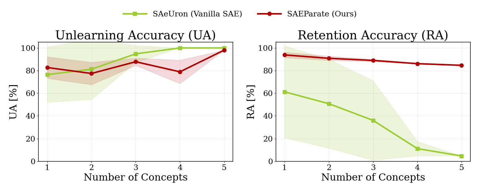
We also provide qualitative results in Figures 11 and 12. SAEParate robustly suppresses multiple target concepts while largely preserving non-target concepts, whereas Vanilla SAE fails to maintain retention after several sequential unlearning requests. These results further suggest that SAEParate reduces redundant feature selection by directly separating latent representations, allowing target concepts to be isolated in more concept-specific features.

Vanilla SAE (SAeUron)

Figure 11: Qualitative visualization of object sequential unlearning for Vanilla SAE (SAeUron). The rows labeled $\mathcal{T}_{1}$ through $\mathcal{T}_{5}$ correspond to the target object classes sequentially unlearned at each step. The “Dogs” and “Fishes” rows are non-target object classes and are used to evaluate retention.

SAEParate (Ours)

Figure 12: Qualitative visualization of object sequential unlearning for SAEParate (Ours). The rows labeled $\mathcal{T}_{1}$ through $\mathcal{T}_{5}$ correspond to the target object classes sequentially unlearned at each step. The “Dogs” and “Fishes” rows are non-target object classes and are used to evaluate retention.

Appendix C Additional Visualizations

C.1 Additional Latent Space Visualizations

To further analyze the structure of the learned latent space, we visualize sparse latent representations using UMAP [29] and measure their concept-wise clustering behavior. The analysis is conducted on the validation set used for computing feature importance scores, which contains 20 prompts per target style, 80 prompts per target object and per target style-object combination for the joint setting. In each UMAP visualization, different colors denote different concepts, following the class and theme categories defined in UnlearnCanvas.

Using the same visualization protocol as the object-level analysis in Figure 2, we first provide the style-level latent visualization in Figure 13. We then visualize the latent space of SAEs trained for joint style-object concepts in Figure 14. Finally, we additionally report the latent space visualizations of the only-$\mathrm{LSC}$ and only-GeLU variants discussed in the ablation study in Section 5.2 with Figure 15.

Across these visualizations, Vanilla SAE exhibits noticeably entangled sparse representations, whereas SAEParate learns a more concept-discriminative latent space with clearer class-wise separation. This suggests that SAEParate reduces co-activation of shared latent features across concepts, thereby mitigating interference during the unlearning process.

Vanilla SAE (SAeUron)

Cluster Rate ($\uparrow$): 0.98, Centroid Margin ($\downarrow$): 0.76

SAEParate (Ours)

Cluster Rate ($\uparrow$): 1.00, Centroid Margin ($\downarrow$): 0.08

Figure 13: UMAP visualization of sparse SAE latent representations for style unlearning: Vanilla SAE (SAeUron) (left) and SAEParate (right). Each color denotes a different style concept from UnlearnCanvas.

Vanilla SAE (SAeUron)

Cluster Rate ($\uparrow$): 0.98, Centroid Margin ($\downarrow$): 0.93

SAEParate (Ours)

Cluster Rate ($\uparrow$): 1.00, Centroid Margin ($\downarrow$): 0.04

Figure 14: UMAP visualization of sparse SAE latent representations for style-object joint unlearning: Vanilla SAE (SAeUron) (left), SAEParate (right). Each color denotes a different style-object concept from UnlearnCanvas.

Vanilla SAE (SAeUron)

Cluster Rate ($\uparrow$): 0.93, Centroid Margin ($\downarrow$): 0.73

only-$\mathrm{LSC}$

Cluster Rate ($\uparrow$): 0.98, Centroid Margin ($\downarrow$): 0.71

only-GeLU

Cluster Rate ($\uparrow$): 0.94, Centroid Margin ($\downarrow$): 0.64

SAEParate (Ours)

Cluster Rate ($\uparrow$): 1.00, Centroid Margin ($\downarrow$): 0.06

Figure 15: UMAP visualization of sparse SAE latent representations for Vanilla SAE (SAeUron) (top-left), only-$\mathrm{LSC}$ (top-right), only-GeLU (bottom-left), and SAEParate (Ours) (bottom-right). Each color denotes a different concept class from UnlearnCanvas.

C.2 Detailed Performance Heatmaps

For measuring the class-wise impact of unlearning, we report classification-accuracy heatmaps over all UnlearnCanvas concepts, including the target concept itself. We provide object-unlearning heatmaps for SAeUron and SAEParate in Figures 16 and 17, respectively, and style-unlearning heatmaps in Figures 18 and 19. As shown in these heatmaps, SAEParate achieves near-perfect unlearning accuracy along the target-concept diagonal while preserving high accuracy for non-target concepts.

Figure 16: Detailed performance heatmap of SAeUron in object unlearning.

Figure 17: Detailed performance heatmap of SAEParate in object unlearning.

Figure 18: Detailed performance heatmap of SAeUron in style unlearning.

Figure 19: Detailed performance heatmap of SAEParate in style unlearning.

C.3 Qualitative Comparisons

We provide qualitative comparisons for object, style, and joint unlearning scenarios, including images generated by the base model, SAeUron, and SAEParate. The results are shown in Figures 20, 21, 22, and 23. Notably, SAEParate preserves non-target concepts more faithfully than SAeUron, with particularly strong retention in the joint unlearning examples shown in Figures 22 and 23.

Figure 20: Qualitative comparison with Vanilla SAE on object unlearning.

Figure 21: Qualitative comparison with Vanilla SAE on style unlearning.

Figure 22: Qualitative comparison with Vanilla SAE on style-object joint unlearning.

Figure 23: Qualitative comparison with Vanilla SAE on style-object joint unlearning.

Appendix D Broader Impacts

This work aims to advance machine learning by improving selective concept unlearning in text-to-image diffusion models. While our method is designed to remove unwanted, biased, or harmful content while preserving non-target concepts, it is inherently dual-use and could be misused for censorship, unfair content suppression, or undesirable manipulation of model behavior. Therefore, real-world deployment should require transparent target definitions, careful evaluation, and appropriate human oversight.

References

- [1] (2023) Towards monosemanticity: decomposing language models with dictionary learning. Transformer Circuits Thread. Note: https://transformer-circuits.pub/2023/monosemantic-features/index.html Cited by: §2, §3.2.
- [2] (2024) BatchTopK sparse autoencoders. External Links: 2412.06410, Link Cited by: §2, §3.2.
- [3] (2025) Learning multi-level features with matryoshka sparse autoencoders. External Links: 2503.17547, Link Cited by: §3.3.
- [4] (2015) Towards making systems forget with machine unlearning. USA, pp. 463–480. External Links: ISBN 9781467369497, Link, Document Cited by: §1, §2.
- [5] (2025) SAEmnesia: erasing concepts in diffusion models with supervised sparse autoencoders. arXiv preprint arXiv:2509.21379. Cited by: §2.
- [6] (2020) A simple framework for contrastive learning of visual representations. pp. 1597–1607. Cited by: §2.
- [7] (2011-11–13 Apr) An analysis of single-layer networks in unsupervised feature learning. In Proceedings of the Fourteenth International Conference on Artificial Intelligence and StatisticsThe Thirty-eight Conference on Neural Information Processing Systems Datasets and Benchmarks TrackProceedings of the 2015 IEEE Symposium on Security and PrivacyThe Thirteenth International Conference on Learning RepresentationsProceedings of the IEEE/CVF conference on computer vision and pattern recognitionThe Twelfth International Conference on Learning RepresentationsProceedings of the IEEE/CVF Conference on Computer Vision and Pattern Recognition (CVPR)Proceedings of the IEEE/CVF Conference on Computer Vision and Pattern RecognitionThe Twelfth International Conference on Learning RepresentationsProceedings of the IEEE/CVF winter conference on applications of computer visionInternational Conference on Learning RepresentationsNeurIPS ML Safety WorkshopProceedings of the IEEE/CVF international conference on computer visionEuropean Conference on Computer VisionProceedings of the IEEE/CVF conference on computer vision and pattern recognitionProceedings of the IEEE/CVF international conference on computer visionInternational conference on machine learningInternational conference on machine learningProceedings of the IEEE/CVF conference on computer vision and pattern recognitionProceedings of the IEEE/CVF conference on computer vision and pattern recognitionProceedings of the 2021 conference on empirical methods in natural language processingEuropean conference on computer vision, G. Gordon, D. Dunson, and M. Dudík (Eds.), Proceedings of Machine Learning ResearchSP ’15, Vol. 15, Fort Lauderdale, FL, USA, pp. 215–223. External Links: Link Cited by: §1, §2.
- [8] (2023) Sparse autoencoders find highly interpretable features in language models. External Links: 2309.08600, Link Cited by: §1, §2.
- [9] (2025) SAeUron: interpretable concept unlearning in diffusion models with sparse autoencoders. In Forty-second International Conference on Machine Learning, External Links: Link Cited by: §A.1, §A.2, §A.3.1, §A.3, §A.6, Table 5, §B.1, Table 11, §1, §2, §3.2, Table 1, §5, §5.
- [10] (2021) An image is worth 16x16 words: transformers for image recognition at scale. External Links: Link Cited by: §5.
- [11] (2024) SalUn: empowering machine unlearning via gradient-based weight saliency in both image classification and generation. External Links: Link Cited by: Table 5, §1, §2, Table 1, §5.
- [12] (2023) Erasing concepts from diffusion models. pp. 2426–2436. Cited by: Table 5, §2, Table 1, §5.
- [13] (2024) Unified concept editing in diffusion models. pp. 5111–5120. Cited by: Table 5, §1, §2, Table 1, §5.
- [14] (2024) Scaling and evaluating sparse autoencoders. External Links: 2406.04093, Link Cited by: §3.2.
- [15] (2023) Finding neurons in a haystack: case studies with sparse probing. Transactions on Machine Learning Research. Note: External Links: ISSN 2835-8856, Link Cited by: §5.2.
- [16] (2020) Momentum contrast for unsupervised visual representation learning. pp. 9729–9738. Cited by: §2.
- [17] (2016) Gaussian error linear units (gelus). arXiv preprint arXiv:1606.08415. Cited by: §1, §4.2.
- [18] (2023) Selective amnesia: a continual learning approach to forgetting in deep generative models. Advances in Neural Information Processing Systems 36, pp. 17170–17194. Cited by: §2.
- [19] (2021) Clipscore: a reference-free evaluation metric for image captioning. pp. 7514–7528. Cited by: §B.3.
- [20] (2017) Gans trained by a two time-scale update rule converge to a local nash equilibrium. Advances in neural information processing systems 30. Cited by: §5.
- [21] (2020) Supervised contrastive learning. Advances in neural information processing systems 33, pp. 18661–18673. Cited by: §2, §4.1, §4.1.
- [22] (2014) Adam: a method for stochastic optimization. arXiv preprint arXiv:1412.6980. Cited by: §A.1.
- [23] (2023) Ablating concepts in text-to-image diffusion models. pp. 22691–22702. Cited by: §A.6, Table 5, §2, Table 1, §5.
- [24] (2025) Sparse autoencoders do not find canonical units of analysis. External Links: 2502.04878, Link Cited by: §1, §3.3.
- [25] (2024) Get what you want, not what you don’t: image content suppression for text-to-image diffusion models. External Links: Link Cited by: Table 5, §1, §2, Table 1, §5.
- [26] (2014) Microsoft coco: common objects in context. pp. 740–755. Cited by: §B.3.
- [27] (2024) One-dimensional adapter to rule them all: concepts diffusion models and erasing applications. pp. 7559–7568. Cited by: Table 5, §1, §2, Table 1, §5.
- [28] (2013) K-sparse autoencoders. CoRR abs/1312.5663. External Links: Link Cited by: §2, §3.2.
- [29] (2018) UMAP: uniform manifold approximation and projection. Journal of Open Source Software 3 (29). Cited by: §C.1, Figure 2.
- [30] (2021) Learning transferable visual models from natural language supervision. pp. 8748–8763. Cited by: §2.
- [31] (2022) Hierarchical text-conditional image generation with clip latents. arXiv preprint arXiv:2204.06125 1 (2), pp. 3. Cited by: §1.
- [32] (2022) Red-teaming the stable diffusion safety filter. External Links: Link Cited by: §1.
- [33] (2022) High-resolution image synthesis with latent diffusion models. pp. 10684–10695. Cited by: §A.1, §B.3, §1, §5.
- [34] (2023) Safe latent diffusion: mitigating inappropriate degeneration in diffusion models. pp. 22522–22531. Cited by: §B.3, §5.2.
- [35] (2024) Scissorhands: scrub data influence via connection sensitivity in networks. pp. 367–384. Cited by: Table 5, §2, Table 1, §5.
- [36] (2025-06) Erasing undesirable influence in diffusion models. pp. 28263–28273. Cited by: Table 5, §1, §2, Table 1, §5.
- [37] (2024) Forget-me-not: learning to forget in text-to-image diffusion models. pp. 1755–1764. Cited by: Table 5, §2, Table 1, §5.
- [38] (2024) UnlearnCanvas: stylized image dataset for enhanced machine unlearning evaluation in diffusion models. External Links: Link Cited by: §A.6, §A.6, §1, §2, Figure 2, §3.1, §5, §5, §5.