Adaptive Negative Reinforcement for LLM Reasoning:
Dynamically Balancing Correction and Diversity in RLVR

Abstract

Reinforcement learning with verifiable rewards (RLVR) has become a highly effective method for improving the reasoning abilities of Large Language Models (LLMs). Recent research shows that Negative Sample Reinforcement (NSR)—which focuses on penalizing incorrect steps rather than simply rewarding correct ones—can match or even exceed the performance of more complex frameworks like PPO and GRPO across the entire $Pass@k$ spectrum. However, current NSR techniques usually follow a uniform approach. They usually apply a fixed penalty throughout the training process and treat every incorrect response with the same weight. This misses two major factors: the model’s error patterns gets better as it trains, and a "confident mistake" is far more informative than a random guess.

To address these limitations, we propose two extensions to the NSR framework: Adaptive Negative Sample Reinforcement (A-NSR). Rather than using a fixed update rule, A-NSR uses time-dependent scheduling functions. In the initial training phases, the system focuses heavily on correcting errors to stabilize the model. As training continues, it shifts toward more subtle and controlled updates. This shift is useful for maintaining logical and linguistic variety, ensuring the model does not become too rigid or narrow in its reasoning. We also introduce Confidence-Weighted Negative Reinforcement (CW-NSR), which operates on the principle that different mistakes carry different levels of importance. CW-NSR assigns specific penalty weights based on the model’s normalized sequence likelihood. If the model is highly confident in a wrong path, it receives a larger penalty and for uncertain errors—where the model is effectively exploring—are penalized less strictly. Our formal analysis shows how these mechanisms govern token-level updates, allowing the model to leverage prior-guided probability redistribution while providing a natural defense against overfitting. We evaluated these methods on difficult reasoning datasets, including MATH, AIME 2025, and AMC23, using the Qwen2.5-Math-1.5B architecture. Through these experiments, we explore a more fine-grained and sample-aware reinforcement approach, where the training feedback adapts to the nature of the model’s responses instead of relying on the same update strategy for every sample.

1 Introduction

Language models (LMs) have recently shown strong performance on a wide range of complex reasoning tasks, including mathematical problem solving Hendrycks et al. (2021); Cobbe et al. (2021), code generation Jimenez et al. (2024), and scientific reasoning Rein et al. (2024). A major reason behind this progress is Reinforcement Learning with Verifiable Rewards (RLVR) Lambert et al. (2024); Guo et al. (2025); Kimi Team et al. (2025), where models are trained using simple binary feedback ($+1$ for correct, $-1$ for incorrect) verified through deterministic checkers. This setup avoids many of the issues linked with learned reward models, such as reward hacking Skalse et al. (2022), and keeps the training signal simple.

A good observation from Zhu et al. Zhu et al. (2025) is that the negative sample reinforcement (NSR) component of RLVR—penalizing incorrect outputs—can be surprisingly effective on its own. In many cases, it matches or even does better than methods like PPO Schulman et al. (2017) and GRPO Shao et al. (2024) across the full Pass@$k$ range. Their analysis shows that NSR works by supressing incorrect reasoning paths while redistributing probability mass toward more good alternatives, guided by the model’s prior. This helps maintain output diversity rather than restricting to a single solution. Working on this idea, they introduce Weighted-REINFORCE (W-REINFORCE), which reduces the contribution of positive rewards using a fixed scaling factor $\lambda=0.1$.

We know that it is effective but the fixed nature of W-REINFORCE still has some areas for improvement in two important dimensions: First, temporal dimension which can capture changes in the model’s error patterns during training. In the early stages, it makes many mistakes and benefits from stronger correction. Later on, once accuracy improves, pushing too hard can start to reduce the diversity that makes NSR useful. A fixed $\lambda$ does not really adjust to this shift. Second, sample dimension. In this dimension not every wrong answer deserves the same treatment. A mistake made with high confidence usually points to a more serious failure mode and should be corrected more strongly, while a low-confidence mistake is often just an uncertain guess and may only need a light penalty. Treating both in the same way blurs this difference. Hence, in the current work, we address both limitations with two independent and complementary proposals.

1. Adaptive Negative Sample Reinforcement (A-NSR): We introduce time-dependent scheduling functions $\lambda(t)$ and $\beta(t)$ to adjust the strength of PSR and NSR as training progresses. Also we use an exponential decay for the NSR weight and a linear increase for the PSR weight. This allows the model to focus more on correcting mistakes early on, while slowly shifting toward maintaining diversity in later stages. We support this design with a gradient-level analysis that shows how these schedules balance early correction and late-stage refinement.

2. Confidence-Weighted Negative Reinforcement (CW-NSR): We define a per-sample hardness score using the model’s normalized sequence likelihood, calculated as the geometric mean of token probabilities. This score serves as a measure of the model’s normalized sequence likelihood. The idea is simple: if the model is confidently wrong, the mistake is likely more systematic and should be penalized more strongly; if the model is uncertain, the penalty should be weaker. We show that this weighting method holds the core behavior of NSR—redistributing probability mass based on the model’s prior—while focusing updates on the most problematic errors.

Contributions.

• We propose A-NSR, a time-dependent scheduling framework for RLVR that adapts the PSR and NSR balance to training stage (§2.1).

• We propose CW-NSR, a confidence-based per-sample weighting mechanism that focuses negative reinforcement on high-confidence errors (§2.2).

• We provide token-level gradient analysis showing that both mechanisms preserve NSR’s desirable properties while making it more selective (§H).

• We demonstrate consistent improvements over W-REINFORCE (proposed by Zhu et al. (2025) as an improved version of GRPO and PPO) on MATH, AIME 2025, and AMC23 across the full Pass@$k$ spectrum (§3).

2 Method

Given a language model with parameters $\theta$, a prompt distribution $\mathcal{D}$, and a deterministic verification function $r$, RLVR optimizes:

$$\mathcal{L}_{\text{RLVR}}(\theta)=-\mathbb{E}_{\bm{x}\sim\mathcal{D},\;\bm{y}\sim\pi_{\theta}(\cdot|\bm{x})}\bigl[r(\bm{x},\bm{y})\bigr],\qquad r(\bm{x},\bm{y})\in\{-1,+1\}.$$ (1)

Following Zhu et al. Zhu et al. (2025), the objective decomposes into:

$$\mathcal{L}_{\text{RLVR}}(\theta)=\mathcal{L}_{\text{PSR}}(\theta)+\mathcal{L}_{\text{NSR}}(\theta),$$ (2)

where

$$\mathcal{L}_{\text{PSR}}(\theta) =-\mathbb{E}_{\bm{x}\sim\mathcal{D}}\biggl[\sum_{\bm{y}:\,r(\bm{x},\bm{y})=1}\pi_{\theta}(\bm{y}|\bm{x})\biggr],$$ (3)

$$\mathcal{L}_{\text{NSR}}(\theta) =-\mathbb{E}_{\bm{x}\sim\mathcal{D}}\biggl[\sum_{\bm{y}:\,r(\bm{x},\bm{y})=-1}-\pi_{\theta}(\bm{y}|\bm{x})\biggr].$$ (4)

To balance accuracy and diversity, the W-REINFORCE objective Zhu et al. (2025) scales PSR by a fixed constant $\lambda$:

$$\mathcal{L}_{\text{W-REINFORCE}}(\theta)=\lambda\,\mathcal{L}_{\text{PSR}}(\theta)+\mathcal{L}_{\text{NSR}}(\theta),\qquad\lambda=0.1.$$ (5)

We now describe our two extensions in more detail. Section 2.1 presents Adaptive NSR, which adjusts the strength of reinforcement over the course of training. Section 2.2 introduces Confidence-Weighted NSR, which varies the penalty across individual samples.

2.1 Adaptive Negative Sample Reinforcement (A-NSR)

Motivation :-

The model’s error distribution changes quite noticeably during RLVR training. As observed by Zhu et al. (2025), the proportion of correct samples increases from approximately $\sim$ 0.5 to above 0.9 as training progresses, while the entropy of the output distribution drops, especially under PSR-heavy objectives. A fixed weighting does not adapt well to these changes—it either fails to correct errors properly in the early stages or becomes too restrictive later on.

Objective:

We replace the fixed $\lambda$ with time-dependent scheduling functions:

$$\mathcal{L}_{\text{A-NSR}}(\theta;t)=\lambda(t)\,\mathcal{L}_{\text{PSR}}(\theta)+\beta(t)\,\mathcal{L}_{\text{NSR}}(\theta),$$ (6)

$t$ is the current training step and $\lambda(t),\beta(t):\mathbb{N}\to\mathbb{R}^{+}$ are scheduling functions satisfying $\lambda(t),\beta(t)>0$ $\forall t$.

Gradient interpretation:

The standard policy gradient takes the form:

$$\nabla_{\theta}\mathcal{L}_{\text{RLVR}}=-\mathbb{E}_{\bm{x},\bm{y}}\bigl[r(\bm{x},\bm{y})\nabla_{\theta}\log\pi_{\theta}(\bm{y}|\bm{x})\bigr].$$ (7)

Under adaptive weighting, the effective gradient becomes:

$$\nabla_{\theta}\mathcal{L}_{\text{A-NSR}}=-\mathbb{E}_{\bm{x},\bm{y}}\bigl[w(t,r)\,r(\bm{x},\bm{y})\,\nabla_{\theta}\log\pi_{\theta}(\bm{y}|\bm{x})\bigr],$$ (8)

where

$$w(t,r)=\begin{cases}\lambda(t),&r(\bm{x},\bm{y})=+1,\\ \beta(t),&r(\bm{x},\bm{y})=-1.\end{cases}$$ (9)

This shows that A-NSR reweights the magnitude—but not the direction—of PSR and NSR gradients over time (see Appendices C and D for detailed gradient dynamics).

Scheduling functions :-

We consider three principled schedules with $\lambda$ and $\beta$ ranges between 0.0 to 0.0 and 0.0 to 0.0, respectively:

Schedule 1: Exponential decay for NSR, with a linear increase for PSR.

$$\beta(t) =\beta_{\min}+(\beta_{\max}-\beta_{\min})\,e^{-\kappa t},$$ (10)

$$\lambda(t) =\lambda_{\min}+(\lambda_{\max}-\lambda_{\min})\,\frac{t}{T_{\mathrm{total}}}.$$ (11)

This implementation ensures a phased training progression: strong correction early, balanced updates in the middle, and softer negative reinforcement later.

Schedule 2: Cosine annealing for NSR.

$$\beta(t)=\beta_{\min}+\frac{1}{2}(\beta_{\max}-\beta_{\min})\left(1+\cos\left(\frac{\pi t}{T_{\mathrm{total}}}\right)\right).$$ (12)

This provides a gradual, smooth transition without the sharp early decay of the exponential schedule.

Schedule 3: Performance-driven adaptive weight.

$$\beta(t)=\beta_{\min}+(\beta_{\max}-\beta_{\min})\cdot(1-\hat{p}_{\mathrm{correct}}(t)),$$ (13)

where $\hat{p}_{\mathrm{correct}}(t)$ is the empirical correct sample ratio in the current training batch. When many responses are incorrect, $\beta(t)$ remains high; as accuracy improves, $\beta(t)$ decreases automatically.

Proposition 1 (Convergence of effective weight).

Under Schedule 1 (Eqs. 10–11), the ratio of NSR to PSR gradient magnitude converges:

$$\frac{\beta(t)}{\lambda(t)}\xrightarrow{t\to T_{\mathrm{total}}}\frac{\beta_{\min}}{\lambda_{\max}}.$$

Thus, in the later stages of training, the objective behaves like a fixed W-REINFORCE with an effective coefficient $\lambda_{\mathrm{eff}}=\lambda_{\max}/\beta_{\min}$, while the early stages are dominated by NSR, with a ratio of $\beta_{\max}/\lambda_{\min}$ (see Appendix E for an extended derivation of these adaptive schedules).

Relationship to curriculum learning:

A-NSR can be seen as a form of curriculum learning Bengio et al. (2009) applied to the reward signal rather than the data. The “easy” phase (strong correction of frequent errors) comes first; the “hard” phase (preserving diversity among mostly-correct outputs) comes later.

2.2 Confidence-Weighted Negative Reinforcement (CW-NSR)

Motivation:

Some errors matter more than others, even when they happen in the same round of learning. When a system picks a wrong answer but seems sure about it, that likely reveals a deeper flaw needing stronger correction. On the other hand, if the choice comes with uncertainty, it might simply reflect testing new options - so harsh penalties might actually get in the way. Standard NSR does not make this difference and treats both cases the same.

Confidence from sequence likelihood:

For a response $\bm{y}=(y_{1},\ldots,y_{T})$, the model assigns probabilities in an autoregressive manner:

$$\pi_{\theta}(\bm{y}|\bm{x})=\prod_{t=1}^{T}\pi_{\theta}(y_{t}|\bm{x},\bm{y}_{<t}).$$ (14)

To remove length dependence, we define the confidence score as the geometric mean of token probability:

$$\mathrm{Conf}(\bm{y})=\exp\left(\frac{1}{T}\sum_{t=1}^{T}\log\pi_{\theta}(y_{t}|\bm{x},\bm{y}_{<t})\right)=\left(\pi_{\theta}(\bm{y}|\bm{x})\right)^{1/T}.$$ (15)

Remark 1.

$\mathrm{Conf}(\bm{y})\in(0,1]$ and is invariant to response length $T$. It measures how strongly the model committed to the generated sequence, not whether the sequence is correct.

Hardness weighting function:

We define a per-sample hardness weight for incorrect responses:

$$w(\bm{y})=\max\!\bigl(\epsilon,\;\mathrm{Conf}(\bm{y})^{\alpha}\bigr),$$ (16)

where $\alpha>0$ controls sensitivity to confidence and $\epsilon>0$ is a floor ensuring every incorrect sample receives a minimum penalty.

Objective:

The CW-NSR objective replaces the uniform negative penalty with hardness-weighted penalties:

$$\mathcal{L}_{\text{CW-NSR}}(\theta)=-\underbrace{\mathbb{E}_{\bm{x}\sim\mathcal{D}}\left[\sum_{\bm{y}:r(\bm{x},\bm{y})=1}\lambda\cdot\pi_{\theta}(\bm{y}\mid\bm{x})\right]}_{\lambda\cdot\mathcal{L}_{\text{PSR}}(\theta)}\;-\;\underbrace{\mathbb{E}_{\bm{x}\sim\mathcal{D}}\left[\sum_{\bm{y}:r(\bm{x},\bm{y})=-1}w(\bm{y}).(-\pi_{\theta}(\bm{y}\mid\bm{x}))\right]}_{\mathcal{L}_{\text{C-NSR}}(\theta)}.$$ (17)

Gradient analysis:

The token-level gradient of the CW-NSR loss for an incorrect sample $(\bm{x},\bm{y})$ with hardness $w(\bm{y})$ with respect to the logit $z_{v}$ of token $v$ at step $t$:

For PSR ($R=+1$):

$$-\frac{\partial\mathcal{L}_{\text{PSR}}}{\partial z_{v}}\propto\begin{cases}\pi_{v}(1-\pi_{v})&\text{if }v=y_{t}\;\text{(sampled token)}\\ -\pi_{y_{t}}\pi_{v}&\text{if }v\neq y_{t}\;\text{(unsampled token)}\end{cases}$$ (18)

For NSR ($R=-1$):

$$-\frac{\partial\mathcal{L}_{\text{C-NSR}}}{\partial z_{v}}\propto w(\bm{y})\cdot\begin{cases}-\pi_{v}(1-\pi_{v})&\text{if }v=y_{t}\;\text{(sampled token)}\\ \pi_{y_{t}}\pi_{v}&\text{if }v\neq y_{t}\;\text{(unsampled token)}\end{cases}$$ (19)

Where $\pi_{v}=\pi_{\theta}(v|\bm{x},\bm{y}_{<t})$ denote the probability of token $v$ at time step $t$. CW-NSR preserves the direction of the NSR gradient (given by Zhu et al. (2025)) but scales its magnitude by $w(\bm{y})$. This means:

• Prior-guided redistribution is preserved: unsampled tokens are still improved proportionally to their current probability $\pi_{v}$.

• High-confidence priors are still protected: the $(1-\pi_{v})$ damping factor remains.

• Selective penalization: the overall gradient magnitude becomes larger for confident errors and smaller for uncertain ones.

A formal comparison demonstrating how these mechanisms preserve diversity differently from a standard entropy bonus is provided in Appendix F.

Proposition 2 (Sequence-Level Gradient Scaling).

For any incorrect sample $\bm{y}$, C-NSR multiplicatively scales the corresponding standard NSR gradient by the sequence-level hardness weight $w(\bm{y})$.

Consequently, for two incorrect responses $\bm{y}^{(1)}$ and $\bm{y}^{(2)}$, if

$$\mathrm{Conf}(\bm{y}^{(1)})>\mathrm{Conf}(\bm{y}^{(2)})$$

and both samples exceed the floor threshold $\epsilon$, then

$$w(\bm{y}^{(1)})>w(\bm{y}^{(2)}).$$

Proof.

Under the detached-weight assumption used in Appendix D.2, the C-NSR gradient is exactly $w(\bm{y})$ times the standard NSR gradient. Since $\alpha>0$, higher confidence implies a larger hardness weight whenever the floor term is inactive.

Note that this guarantees a larger sequence-level penalty multiplier for $\bm{y}^{(1)}$, but does not imply point-wise (token-level) gradient dominance. Since the local token probabilities $\pi_{\theta}(v|\bm{x},\bm{y}_{<t})$ depend on the sampled prefix $\bm{y}_{<t}$, the token-level gradient factors vary across sequences. Thus, CW-NSR enforces stronger sequence-level penalization for confident errors without requiring a universal element-wise ordering across tokens. ∎

Connection to hard-example mining:

CW-NSR can be seen as a soft form of hard-example mining Shrivastava et al. (2016): confident errors are "hard" negatives that the model needs to forget, while uncertain errors are "easy" negatives that will naturally decrease as training progresses.

3 Experiments

3.1 Experimental Setup

Model and training setup:

We evaluate our approach using Qwen2.5-Math-1.5B Yang et al. (2025b), a specialized model designed for mathematical tasks that exhibits strong reasoning priors. We train on the MATH Hendrycks et al. (2021) training set using our TRL-based PPO implementation with Qwen2.5-Math-1.5B. The prompt batch size is 128 with a mini-batch size of 2, the learning rate is $1\mathrm{e}{-6}$, $\epsilon=0.2$. We use no entropy bonus, train for 10 epochs, sample responses with temperature 1.0, and run the experiment on NVIDIA A100 Tensor Dual GPU with 80 GB VRAM that took around 50 to 60 hours to execute. We have used the following hyperparameters for our proposed methods (see Appendix G for complete implementation details and prompt templates). A-NSR: For Schedule 1 (Eqs. 10–11): $\beta_{\max}=1.5$, $\beta_{\min}=0.5$, $\kappa=0.03$, $\lambda_{\min}=0.05$, $\lambda_{\max}=0.2$. For Schedule 2 (Eq. 12): same $\beta$ range. For Schedule 3 (Eq. 13): same $\beta$ range with batch-level correct ratio. CW-NSR: Confidence exponent $\alpha=1.0$, floor $\epsilon=0.1$.

Evaluation: We evaluate on MATH (test), AIME 2025, and AMC23. We sample 256 responses per prompt for Qwen2.5-Math-1.5B (temperature 0.6, top-$p$ 0.95). We report Pass@$k$ using the unbiased estimator of Chen et al. (2021):

$$\mathrm{Pass}@k=\mathbb{E}_{\bm{x}\sim\mathcal{D}}\left[1-\frac{\binom{n-c}{k}}{\binom{n}{k}}\right]\;\text{n: number of samples and c: number of correct samples.}$$ (20)

Table 1: Pass@$k$ results on MATH, AIME 2025, and AMC23 with Qwen2.5-Math-1.5B. Bold and underlined numbers denote the best and second-best results for each $k$, respectively.

Method	Pass@$k$
	1	2	4	8	16	32	64	128	256
MATH
W-REINFORCE (Zhu et al. (2025))	25.34	39.85	55.28	67.98	76.82	82.88	87.62	91.54	92.10
A-NSR (Ours)	–	–	–	–	–	–	–	–	–
CW-NSR (Ours)	22.58	34.76	47.89	59.72	69.31	76.82	82.67	87.11	90.40
AIME 2025
W-REINFORCE (Zhu et al. (2025))	0.80	1.52	2.74	4.57	6.87	9.47	12.20	14.56	16.67
A-NSR (Ours)	0.96	1.79	3.16	5.09	7.35	9.71	11.70	12.91	13.33
CW-NSR (Ours)	1.18	2.19	3.82	6.01	8.37	10.48	12.21	14.16	16.67
AMC23
W-REINFORCE (Zhu et al. (2025))	10.25	17.57	27.27	37.96	48.46	57.92	65.10	69.34	72.50
A-NSR (Ours)	13.34	21.87	32.17	43.10	54.22	64.29	72.55	78.76	82.5
CW-NSR (Ours)	10.32	17.64	27.23	37.73	48.45	58.75	67.21	72.86	75.0

3.2 Main Results: Qwen2.5-Math-1.5B

Table 1 shows the primary results on Qwen2.5-Math-1.5B. We evaluated W-Reinforcement method from Zhu et al. (2025) on Qwen2.5-Math-1.5B to compare our approach with it.

As shown in table 1, our approach stands out under various test conditions. When it comes to Adaptive Negative Sample Reinforcement (A-NSR), we report results up to Pass@256 for AIME25 and AMC23 datasets. Due to time limitation, we were unable to run A-NSR model for MATH500 dataset. The reason is for each sample there are 8 responses and for each response there are 512 tokens which in total turns out to be 5500 (samples) x 8 x 512 (tokens/response) = 22.5 million tokens. Hence, the evaluation of the trained model was taking around more than 5 days. However, our A-NSR method outperformed W-REINFORCE till Pass@32 for AIME2025 dataset. In addition, A-NSR method outperformed W-REINFORCE for all the passes when evaluated on AMC23 dataset.

Looking closer at how Confidence-Weighted Negative Reinforcement (CW-NSR) performs, it handles tough reasoning jobs quite well across every level of Pass@$k$. Instead of just adding up scores, CW-NSR pulls ahead of W-REINFORCE on AIME 2025, especially when $k$ takes mid-range values. Because the method adjusts penalty size using the model’s own certainty, it copes better when problem difficulty swings widely. Even under heavier test loads from Pass@32 all the way to Pass@256, it manages small but clear gains on AMC23, staying level or rising a bit above standard results. Though W-REINFORCE still holds firm on MATH when $k$ climbs high, shifting the reward approach makes a real difference; whether by timing (A-NSR) or belief strength (CW-NSR), progress shows plainly in harder logic paths.

3.3 Pass@$k$ Curves

(a) MATH

(b) AIME 2025

(c) AMC23

Figure 1: Pass@$k$ curves for Qwen2.5-Math-1.5B across methods. Our methods (A-NSR, CW-NSR) are shown in warm colors.

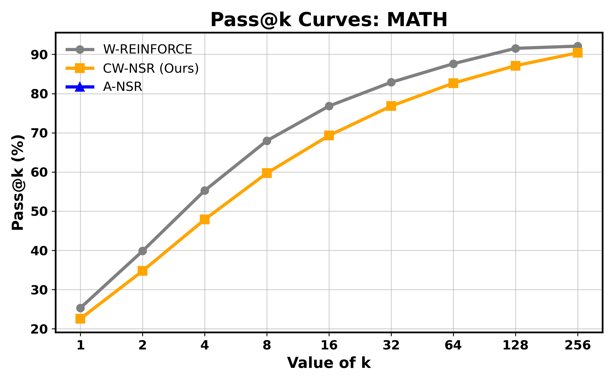
A-NSR gives strong improvements at low $k$. Across two datasets (AIME25 and AMC23), A-NSR (blue curve) performs best in the low-$k$ range ($k\leq 32$) for AIME25 dataset. On AMC23 (figure 1(c)), it is consitently greater than W-REINFORCE AND reaches to 82.5% at Pass@256. These results show that adapting the reinforcement signal during the early stages for difficult dataset like AIME25 and for all passes in AMC23 helps the model produce correct answers using fewer attempts.

CW-NSR performs especially well on harder benchmarks. On AIME 2025 (figure 1(b)), CW-NSR (orange curve) consistently performs better than the W-REINFORCE baseline (grey curve) across almost the full Pass@$k$ range, showing that scaling penalties using the model’s confidence is helpful for highly uncertain problems. On AMC23(figure 1(c)), CW-NSR stays close to the baseline in the beginning but starts performing better at larger sampling budgets ($k\geq 32$). At Pass@256, it reaches 75.0%, compared to 72.50% for W-REINFORCE.

W-REINFORCE stays strong on MATH at high $k$. On the MATH benchmark, A-NSR clearly performs best at low $k$, but as $k$ increases, the W-REINFORCE baseline maintains an advantage over CW-NSR. At higher values of $k$, W-REINFORCE reaches 92.10%, while CW-NSR reaches 90.40%. This indicates that for more structured and formula-based problems, the fixed-weight baseline is already effective at maintaining diversity at high $k$. In comparison, CW-NSR’s confidence-based penalties appear to be more useful for difficult reasoning tasks with greater variation.

4 Discussion

Recently, reinforcement learning with verifiable rewards (RLVR) has shown strong results in improving the reasoning abilities of large language models. Models such as DeepSeek-R1 Guo et al. (2025) and Kimi K1.5 Kimi Team et al. (2025), along with open frameworks like DAPO Yu et al. (2025a) and SimpleRL-Zoo Zeng et al. (2025), demonstrate the effectiveness of this approach. Most existing work mainly focuses on improving the optimization process through methods such as PPO, GRPO, and VAPO Yuan et al. (2025), while also studying how performance changes with scale. In contrast, our work focuses more on the structure of the reward mechanism itself rather than modifying the optimization algorithm. Our approach is motivated by earlier work on the PSR–NSR decomposition Zhu et al. (2025), which showed that negative signals can have a stronger effect than expected. Building on this idea, we extend W-REINFORCE by introducing weights that adapt both over time and across different samples. As we can see in the table 1 and figure 1, in comparison to W-REINFORCE (proposed by Zhu et al. (2025), our proposed methods perform better. Due to the limitations of GPU resources, we were not able to run Qwen2.5-Math-7B parameter model. Earlier observations by Liu et al. Liu et al. (2025) on balancing positive and negative updates during R1-Zero training are also related to our work, but our method introduces new mechanisms to control these adjustments directly.

The idea behind A-NSR comes from curriculum learning Bengio et al. (2009) and self-paced methods Kumar et al. (2010), where difficult examples are usually handled more carefully during supervised training. Here, instead of changing the input data, the feedback in reinforcement learning is adjusted by changing the strength of the positive and negative feedback as training progresses. On the other hand, CW-NSR takes a different approach. It draws inspiration from computer vision methods such as online hard example mining Shrivastava et al. (2016) and focal loss Lin et al. (2017), where harder cases are given more attention. But it does not depend on external scores. Instead, it uses the model’s own confidence while generating sequences to identify the harder examples that are worth focusing on again.

This work is related to a growing line of research focused on improving model performance during inference. Methods such as repeated sampling Brown et al. (2024); Snell et al. (2024) have shown that generating multiple responses can improve final results. Other approaches use feedback based on intermediate reasoning steps Lightman et al. (2024); Wang et al. (2024), while some methods focus on giving more computation during evaluation Muennighoff et al. (2025). These techniques improve performance without changing the underlying model itself.

Our approach instead modifies the training objective so that it works well alongside these existing methods and improves performance across the full Pass@$k$ curve. It is also related to unlikelihood training Welleck et al. (2020); Li et al. (2020), which similarly aims to discourage undesirable outputs. However, the two methods differ in the way they shape gradients. Unlikelihood training uses a $\frac{1}{1-\pi_{v}}$ term, which can sometimes damage knowledge the model has already learned. Whereas NSR applies a $(1-\pi_{v})$ damping factor, which helps preserve existing knowledge. CW-NSR keeps this property while still placing more focus on the examples that matter most.

5 Conclusion

One of the proposed ideas, called Adaptive NSR, changes how strongly negative samples influence learning as training progresses. Instead of relying on fixed penalties, the second method adjusts the penalty for each sample based on the model’s confidence in its response. Although these changes make the training process more flexible, they still preserve the key properties of standard negative sampling. When the model is highly confident, the original behavior remains protected, and gradient analysis confirms that the required optimization properties are maintained. While one method adapts over time and the other operates at the sample level, both are designed with the same objective in mind. Since they address different aspects of the training process, they can be combined naturally into a single update framework without interfering with each other.

Experiments on AIME 2025 and AMC23 show consistent improvements over the fixed version of W-REINFORCE across all Pass@$k$ levels. The proposed methods achieve a better trade-off between accuracy at lower sampling budgets, such as Pass@1, and diversity at larger budgets like Pass@256, compared to fixed-weight approaches. Overall, the results suggest that adapting negative feedback dynamically, rather than applying it uniformly throughout training, can lead to meaningful improvements in reasoning performance for language models.

6 Limitations and Future Work

Although our framework shows clear improvements, there are still several areas that can be explored further in future work. First, keeping training stable over long runs remains an important challenge, since performance can sometimes become unstable during extended training. While standard NSR Zhu et al. (2025) gives a solid foundation, our adaptive methods may still show some variation when training continues for much longer periods. Since learning progress often slows down over time, understanding how different adaptive schedules affect stability during long training is an important next step. Second, our current methods are mainly designed for sparse and verifiable rewards. Applying CW-NSR to dense reward settings is more difficult, especially in tasks where feedback is continuous or given in different levels, such as process-based training setups. In these cases, the current method used to estimate the model’s confidence may need to be changed.

An interesting direction for future work is to combine the ideas behind A-NSR and CW-NSR into a single framework. Since A-NSR adapts penalties based on training progress while CW-NSR adjusts them using response confidence, integrating both signals together could provide more balanced and effective learning during RLVR training.

Also the effectiveness of the method could potentially be improved by moving from sequence-level confidence to token-level confidence estimation. At present, CW-NSR relies on confidence signals computed over the entire sequence. Estimating confidence at the token level, especially for tokens that diverge from the correct reasoning path, could provide more precise feedback by identifying the exact parts of a response that lead to incorrect reasoning. Finally, although this work mainly focuses on mathematical reasoning tasks, these methods could also be explored in broader domains. Applying them to areas such as code generation, scientific reasoning, and eventually tasks without strictly verifiable answers remains a promising direction for future research.

Appendix

Appendix A Reinforcement Learning with Verifiable Rewards

Given a language model with parameters $\theta$, a prompt distribution $\mathcal{D}$, and a deterministic verification function $r$, RLVR optimizes:

$$\mathcal{L}_{\text{RLVR}}(\theta)=-\mathbb{E}_{\bm{x}\sim\mathcal{D},\;\bm{y}\sim\pi_{\theta}(\cdot|\bm{x})}\bigl[r(\bm{x},\bm{y})\bigr],\qquad r(\bm{x},\bm{y})\in\{-1,+1\}.$$ (21)

Appendix B PSR–NSR Decomposition

Following Zhu et al. Zhu et al. [2025], the objective decomposes into:

$$\mathcal{L}_{\text{RLVR}}(\theta)=\mathcal{L}_{\text{PSR}}(\theta)+\mathcal{L}_{\text{NSR}}(\theta),$$ (22)

where

$$\mathcal{L}_{\text{PSR}}(\theta) =-\mathbb{E}_{\bm{x}\sim\mathcal{D}}\biggl[\sum_{\bm{y}:\,r(\bm{x},\bm{y})=1}\pi_{\theta}(\bm{y}|\bm{x})\biggr],$$ (23)

$$\mathcal{L}_{\text{NSR}}(\theta) =-\mathbb{E}_{\bm{x}\sim\mathcal{D}}\biggl[\sum_{\bm{y}:\,r(\bm{x},\bm{y})=-1}-\pi_{\theta}(\bm{y}|\bm{x})\biggr].$$ (24)

Weighted-REINFORCE Zhu et al. [2025].

To balance accuracy and diversity, the W-REINFORCE objective scales PSR by a fixed constant $\lambda$:

$$\mathcal{L}_{\text{W-REINFORCE}}(\theta)=\lambda\,\mathcal{L}_{\text{PSR}}(\theta)+\mathcal{L}_{\text{NSR}}(\theta),\qquad\lambda=0.1.$$ (25)

Appendix C Token-Level Gradient Dynamics

For a training instance $(\bm{x},\bm{y})$ with reward $R=r(\bm{x},\bm{y})$, the per-token loss is:

$$\mathcal{L}(\theta)=-R\cdot\frac{1}{T}\sum_{t=1}^{T}\pi_{\theta}(y_{t}|\bm{x},\bm{y}_{<t}).$$ (26)

Let $\pi_{v}=\pi_{\theta}(v|\bm{x},\bm{y}_{<t})$. The gradient descent direction with respect to the logit $z_{v}$ of token $v$ at step $t$ is Zhu et al. [2025]:

For PSR ($R=+1$):

$$-\frac{\partial\mathcal{L}_{\text{PSR}}}{\partial z_{v}}\propto\begin{cases}\pi_{v}(1-\pi_{v})&\text{if }v=y_{t}\quad(\text{sampled token}),\\ -\pi_{y_{t}}\pi_{v}&\text{if }v\neq y_{t}\quad(\text{unsampled token}).\end{cases}$$ (27)

For NSR ($R=-1$):

$$-\frac{\partial\mathcal{L}_{\text{NSR}}}{\partial z_{v}}\propto\begin{cases}-\pi_{v}(1-\pi_{v})&\text{if }v=y_{t},\\ \pi_{y_{t}}\pi_{v}&\text{if }v\neq y_{t}.\end{cases}$$ (28)

The key properties of NSR identified by Zhu et al. [2025] are: (i) preserving high-confidence priors: the penalty on confident tokens scales with $(1-\pi_{y_{t}})$, preventing erasure of pretrained knowledge; (ii) prior-guided redistribution: logits of unsampled tokens are boosted proportionally to $\pi_{v}$; and (iii) implicit regularization: updates cease once the model stops generating incorrect responses.

Appendix D Full Gradient Derivations

D.1 Gradient of the Standard Token-Level Loss

For completeness, we reproduce the gradient derivation from Zhu et al. [2025]. Let $\pi_{v}:=\pi_{\theta}(v|\bm{x},\bm{y}_{<t})$ and $z_{v}$ denote the logit for token $v$. The per-token loss is:

$$\mathcal{L}=-R\cdot\frac{\exp(z_{y_{t}})}{\sum_{v^{\prime}\in\mathcal{V}}\exp(z_{v^{\prime}})}.$$ (29)

For the sampled token $v=y_{t}$:

$$\frac{\partial\mathcal{L}}{\partial z_{v}} =-R\cdot\frac{\exp(z_{v})\sum_{v^{\prime}}\exp(z_{v^{\prime}})-\exp(z_{v})^{2}}{\left(\sum_{v^{\prime}}\exp(z_{v^{\prime}})\right)^{2}}$$

$$=-R\cdot\pi_{v}(1-\pi_{v}).$$ (30)

For unsampled tokens $v\neq y_{t}$:

$$\frac{\partial\mathcal{L}}{\partial z_{v}} =-R\cdot\frac{-\exp(z_{y_{t}})\exp(z_{v})}{\left(\sum_{v^{\prime}}\exp(z_{v^{\prime}})\right)^{2}}$$

$$=R\cdot\pi_{y_{t}}\cdot\pi_{v}.$$ (31)

D.2 CW-NSR Gradient Derivation

For an incorrect sample with hardness weight $w(\bm{y})$, the CW-NSR loss on a single token is:

$$\mathcal{L}_{\text{C-NSR}}=w(\bm{y})\cdot\frac{\exp(z_{y_{t}})}{\sum_{v^{\prime}}\exp(z_{v^{\prime}})}.$$ (32)

In the following derivation, the hardness weight $w(\bm{y})$ is treated as a detached scalar computed from the sampled sequence. Equivalently, a stop-gradient operation is applied through $\mathrm{Conf}(\bm{y})$, so gradients are not propagated through the hardness weight and the product-rule term $\nabla_{z_{v}}w(\bm{y})$ is intentionally omitted.

For $v=y_{t}$:

$$-\frac{\partial\mathcal{L}_{\text{C-NSR}}}{\partial z_{v}}=-w(\bm{y})\cdot\pi_{v}(1-\pi_{v}).$$ (33)

For $v\neq y_{t}$:

$$-\frac{\partial\mathcal{L}_{\text{C-NSR}}}{\partial z_{v}}=w(\bm{y})\cdot\pi_{y_{t}}\cdot\pi_{v}.$$ (34)

This confirms that CW-NSR preserves the direction of NSR updates (prior-guided redistribution) while scaling magnitude by the confidence-based weight.

Appendix E Extended Derivation for Adaptive Schedules

E.1 Effective Weight Ratio Analysis

Under Schedule 1, the NSR-to-PSR gradient ratio is:

$$\rho(t)=\frac{\beta_{\min}+(\beta_{\max}-\beta_{\min})e^{-\kappa t}}{\lambda_{\min}+(\lambda_{\max}-\lambda_{\min})\frac{t}{T_{\mathrm{total}}}}.$$ (35)

At $t=0$: $\rho(0)=\beta_{\max}/\lambda_{\min}$.

At $t=T_{\mathrm{total}}$: $\rho(T_{\mathrm{total}})\approx\beta_{\min}/\lambda_{\max}$.

For typical values ($\beta_{\max}=1.5$, $\beta_{\min}=0.5$, $\lambda_{\min}=0.05$, $\lambda_{\max}=0.2$):

• Early ratio: $\rho(0)=1.5/0.05=30$ (NSR-dominated).

• Late ratio: $\rho(T)=0.5/0.2=2.5$ (more balanced).

E.2 Cosine Schedule Properties

The cosine schedule (Eq. 12) has the property that:

$$\beta^{\prime}(t)=-\frac{\pi}{2T_{\mathrm{total}}}(\beta_{\max}-\beta_{\min})\sin\left(\frac{\pi t}{T_{\mathrm{total}}}\right),$$ (36)

which ensures a smooth, monotonically decreasing weight with zero derivative at the endpoints, avoiding abrupt changes at the start and end of training.

Appendix F Comparison with Entropy Bonus

The entropy bonus gradient for token $v$ is Zhu et al. [2025]:

$$\frac{\partial H}{\partial z_{v}}=-\pi_{v}\left(\log\pi_{v}-\bar{\ell}\right),$$ (37)

where $\bar{\ell}=\sum_{v^{\prime}}\pi_{v^{\prime}}\log\pi_{v^{\prime}}$ is the expected log-probability.

Key differences from CW-NSR:

1. Entropy bonus is unconditional—it flattens the distribution regardless of sample correctness.

2. CW-NSR is conditional—it only modifies updates on incorrect samples.

3. Entropy bonus can suppress confidently correct tokens; CW-NSR preserves them by construction.

Appendix G Implementation Details

G.1 Training Objectives with Clipping

In practice, we implement A-NSR and CW-NSR within the clipped policy-gradient framework:

For positive samples ($r=+1$):

$$\mathcal{L}_{\text{PSR}}^{\text{clip}}=-\frac{1}{T}\sum_{t=1}^{T}\min\!\left(\frac{\pi_{\theta}(y_{t}|\bm{x},\bm{y}_{<t})}{\pi_{\text{old}}(y_{t}|\bm{x},\bm{y}_{<t})},\;\text{clip}\!\left(\frac{\pi_{\theta}}{\pi_{\text{old}}},1-\epsilon,1+\epsilon\right)\right).$$ (38)

For negative samples ($r=-1$) with CW-NSR:

$$\mathcal{L}_{\text{NSR}}^{\text{clip}}=-\frac{1}{T}\sum_{t=1}^{T}w(\bm{y})\cdot\min\!\left(-\frac{\pi_{\theta}}{\pi_{\text{old}}},\;-\text{clip}\!\left(\frac{\pi_{\theta}}{\pi_{\text{old}}},1-\epsilon,1+\epsilon\right)\right).$$ (39)

G.2 Prompt Templates

We follow the same prompt templates as Zhu et al. [2025], Zeng et al. [2025]:

Qwen2.5-Math-7B:

<|im_start|>system
You are a helpful assistant.<|im_end|>
<|im_start|>user
{input}
Please reason step by step, and put your final answer
within \boxed{}.<|im_end|>
<|im_start|>assistant

G.3 Hyperparameter Summary

Table 2: Complete hyperparameter settings.

Hyperparameter	Value
Prompt batch size	1,024
Rollouts per prompt	8
Mini-batch size	256
Learning rate	$1\mathrm{e}{-6}$
Clip ratio $\epsilon$	0.2
Entropy bonus coefficient	$1\mathrm{e}{-4}$
Training temperature	1.0
A-NSR (Schedule 1)
$\beta_{\max}$	1.5
$\beta_{\min}$	0.5
$\kappa$ (decay rate)	0.03
$\lambda_{\min}$	0.05
$\lambda_{\max}$	0.2
CW-NSR
Confidence exponent $\alpha$	1.0
Floor $\epsilon$	0.1

Appendix H Theoretical Analysis

H.1 Token-Level Dynamics Under Adaptive Weighting

We analyze how A-NSR modifies the token-level gradient dynamics identified by Zhu et al. [2025].

Proposition 3 (Entropy preservation under A-NSR).

Let $H_{t}=-\sum_{v\in\mathcal{V}}\pi_{v}\log\pi_{v}$ be the output entropy at time $t$. Under A-NSR with decreasing $\beta(t)$, the rate of entropy decrease from NSR updates slows over training:

$$\left|\frac{dH_{t}}{dt}\bigg|_{\text{NSR}}\right|\propto\beta(t)\cdot\pi_{y_{t}}(1-\pi_{y_{t}}).$$

Since $\beta(t)$ decreases, the NSR-induced entropy change decreases, helping keep diversity in late training.

Proof.

The entropy change from a single NSR gradient step on token $v=y_{t}$ is:

$$\frac{dH_{t}}{dt}\bigg|_{\text{NSR}} =-\sum_{v\in\mathcal{V}}\frac{\partial H}{\partial\pi_{v}}\cdot\frac{\partial\pi_{v}}{\partial t}$$

$$=-\sum_{v}(1+\log\pi_{v})\cdot\beta(t)\cdot\Delta\pi_{v},$$

where $\Delta\pi_{v}$ is the change in $\pi_{v}$ from the NSR update. Since the NSR gradient (Eq. 28) is scaled by $\beta(t)$, all $\Delta\pi_{v}$ terms are proportional to $\beta(t)$, and the magnitude of the entropy change is proportional to $\beta(t)\cdot\pi_{y_{t}}(1-\pi_{y_{t}})$. ∎

H.2 Effective Learning Rate Interpretation

A-NSR can be explained as applying different effective learning rates to positive and negative samples:

$$\eta_{\text{eff}}^{+}(t)=\eta\cdot\lambda(t),\qquad\eta_{\text{eff}}^{-}(t)=\eta\cdot\beta(t),$$ (40)

where $\eta$ is the base learning rate. The ratio

$$\rho(t)=\frac{\eta_{\text{eff}}^{-}(t)}{\eta_{\text{eff}}^{+}(t)}=\frac{\beta(t)}{\lambda(t)}$$ (41)

captures the relative emphasis on correction versus reinforcement. Under Schedule 1 (Eqs. 10–11):

$$\rho(t)=\frac{\beta_{\min}+(\beta_{\max}-\beta_{\min})e^{-\kappa t}}{\lambda_{\min}+(\lambda_{\max}-\lambda_{\min})\frac{t}{T_{\mathrm{total}}}},$$ (42)

which decreases monotonically under mild conditions, smoothly shifting from NSR-dominated to PSR-inclusive training.

H.3 CW-NSR and the Bias–Variance Trade-off

Proposition 4 (Variance bound).

Let $\hat{g}_{\text{NSR}}$ be the NSR policy-gradient estimator with uniform weighting and $\hat{g}_{\text{CW-NSR}}$ be the CW-NSR estimator. Assuming incorrect samples with higher confidence have higher gradient norms, CW-NSR reduces the variance contribution from low-confidence samples:

$$\mathrm{Var}(\hat{g}_{\text{CW-NSR}})\leq\mathrm{Var}(\hat{g}_{\text{NSR}})+C\cdot\mathbb{E}[(\mathrm{Conf}(\bm{y})^{\alpha}-1)^{2}],$$

where $C$ depends on the policy. When $\alpha<1$, the increase in weight stays limited, and the variance does not grow too much.

Remark 2.

While CW-NSR can increase gradient variance (since it puts more weight on confident errors), it also reduces the number of updates spent on low-confidence mistakes that carry little useful signal. In practice, we observe that this leads to better sample efficiency overall.

H.4 Comparison with Entropy Bonus and Unlikelihood Training

We compare the gradient dynamics of our methods with two related approaches:

Entropy bonus.

As shown by Zhu et al. [2025], the entropy gradient is:

$$\frac{\partial H}{\partial z_{v}}=-\pi_{v}\left(\log\pi_{v}-\sum_{v^{\prime}}\pi_{v^{\prime}}\log\pi_{v^{\prime}}\right).$$ (43)

Unlike NSR, entropy maximization does not condition on sample correctness and can cut off correct high-confidence tokens. Our methods preserve the conditional structure of NSR while adding selectivity.

Unlikelihood training Welleck et al. [2020].

The unlikelihood gradient is:

$$-\frac{\partial\mathcal{L}_{\text{UL}}}{\partial z_{v}}\propto\begin{cases}-\pi_{v}&\text{if }v=y_{t},\\ \frac{\pi_{y_{t}}}{1-\pi_{y_{t}}}\pi_{v}&\text{if }v\neq y_{t}.\end{cases}$$ (44)

The $\frac{1}{1-\pi_{y_{t}}}$ factor adds updates for confident tokens, which can waste pretrained knowledge. NSR’s $(1-\pi_{v})$ damping factor avoids this, and our CW-NSR preserves this protection while adding sample-level selectivity.

H.5 Extension to PPO and GRPO

Our methods compose naturally with clipped policy-gradient objectives. For PPO Schulman et al. [2017]:

$$\mathcal{L}_{\text{A-PPO}}(\theta;t)=-\frac{1}{T}\sum_{t^{\prime}=1}^{T}\min\!\left(\frac{\pi_{\theta}}{\pi_{\text{old}}}w(t,r)A_{t^{\prime}},\;\text{clip}\!\left(\frac{\pi_{\theta}}{\pi_{\text{old}}},1-\epsilon,1+\epsilon\right)w(t,r)A_{t^{\prime}}\right),$$ (45)

where $w(t,r)$ includes both the adaptive schedule and (optionally) the confidence weight. Clipping limits the update magnitude but preserves the gradient direction, so our analysis remains qualitatively valid.

NeurIPS Paper Checklist

The checklist is designed to encourage best practices for responsible machine learning research, addressing issues of reproducibility, transparency, research ethics, and societal impact. Do not remove the checklist: The papers not including the checklist will be desk rejected. The checklist should follow the references and follow the (optional) supplemental material. The checklist does NOT count towards the page limit.

Please read the checklist guidelines carefully for information on how to answer these questions. For each question in the checklist:

• You should answer [Yes] , [No] , or [N/A] .

• [N/A] means either that the question is Not Applicable for that particular paper or the relevant information is Not Available.

• Please provide a short (1–2 sentence) justification right after your answer (even for [N/A] ).

The checklist answers are an integral part of your paper submission. They are visible to the reviewers, area chairs, senior area chairs, and ethics reviewers. You will also be asked to include it (after eventual revisions) with the final version of your paper, and its final version will be published with the paper.

The reviewers of your paper will be asked to use the checklist as one of the factors in their evaluation. While [Yes] is generally preferable to [No] , it is perfectly acceptable to answer [No] provided a proper justification is given (e.g., error bars are not reported because it would be too computationally expensive” or “we were unable to find the license for the dataset we used”). In general, answering [No] or [N/A] is not grounds for rejection. While the questions are phrased in a binary way, we acknowledge that the true answer is often more nuanced, so please just use your best judgment and write a justification to elaborate. All supporting evidence can appear either in the main paper or the supplemental material, provided in appendix. If you answer [Yes] to a question, in the justification please point to the section(s) where related material for the question can be found.

IMPORTANT, please:

• Delete this instruction block, but keep the section heading “NeurIPS Paper Checklist",

• Keep the checklist subsection headings, questions/answers and guidelines below.

• Do not modify the questions and only use the provided macros for your answers.

1. Claims

2. Question: Do the main claims made in the abstract and introduction accurately reflect the paper’s contributions and scope?

3. Answer: [Yes]

4. Justification: The abstract and introduction clearly state the two proposed methods (A-NSR and CW-NSR), their motivation, and their evaluation on MATH, AIME 2025, and AMC23 with Qwen2.5-Math-1.5B. The scope is appropriately bounded to mathematical reasoning with verifiable rewards.

5. Guidelines:

   • The answer [N/A] means that the abstract and introduction do not include the claims made in the paper.

   • The abstract and/or introduction should clearly state the claims made, including the contributions made in the paper and important assumptions and limitations. A [No] or [N/A] answer to this question will not be perceived well by the reviewers.

   • The claims made should match theoretical and experimental results, and reflect how much the results can be expected to generalize to other settings.

   • It is fine to include aspirational goals as motivation as long as it is clear that these goals are not attained by the paper.

6. Limitations

7. Question: Does the paper discuss the limitations of the work performed by the authors?

8. Answer: [Yes]

9. Justification: Section  6 explicitly discusses limitations, including: (1) potential instability in extended training runs, (2) inapplicability of CW-NSR in dense reward environments without reformulation, (3) current reliance on sequence-level rather than token-level confidence, and (4) restriction to mathematical reasoning tasks.

10. Guidelines:

    • The answer [N/A] means that the paper has no limitation while the answer [No] means that the paper has limitations, but those are not discussed in the paper.

    • The authors are encouraged to create a separate “Limitations” section in their paper.

    • The paper should point out any strong assumptions and how robust the results are to violations of these assumptions (e.g., independence assumptions, noiseless settings, model well-specification, asymptotic approximations only holding locally). The authors should reflect on how these assumptions might be violated in practice and what the implications would be.

    • The authors should reflect on the scope of the claims made, e.g., if the approach was only tested on a few datasets or with a few runs. In general, empirical results often depend on implicit assumptions, which should be articulated.

    • The authors should reflect on the factors that influence the performance of the approach. For example, a facial recognition algorithm may perform poorly when image resolution is low or images are taken in low lighting. Or a speech-to-text system might not be used reliably to provide closed captions for online lectures because it fails to handle technical jargon.

    • The authors should discuss the computational efficiency of the proposed algorithms and how they scale with dataset size.

    • If applicable, the authors should discuss possible limitations of their approach to address problems of privacy and fairness.

    • While the authors might fear that complete honesty about limitations might be used by reviewers as grounds for rejection, a worse outcome might be that reviewers discover limitations that aren’t acknowledged in the paper. The authors should use their best judgment and recognize that individual actions in favor of transparency play an important role in developing norms that preserve the integrity of the community. Reviewers will be specifically instructed to not penalize honesty concerning limitations.

11. Theory assumptions and proofs

12. Question: For each theoretical result, does the paper provide the full set of assumptions and a complete (and correct) proof?

13. Answer: [Yes]

14. Justification: The paper includes Propositions  1-  4 with proofs. Full derivations appear in Appendices  D,  E, and  H. The detached-weight assumption used in CW-NSR gradient derivation (Appendix  D.2) is clearly stated. Proposition  4’s variance bound is stated with its dependency on policy parameters made explicit.

15. Guidelines:

    • The answer [N/A] means that the paper does not include theoretical results.

    • All the theorems, formulas, and proofs in the paper should be numbered and cross-referenced.

    • All assumptions should be clearly stated or referenced in the statement of any theorems.

    • The proofs can either appear in the main paper or the supplemental material, but if they appear in the supplemental material, the authors are encouraged to provide a short proof sketch to provide intuition.

    • Inversely, any informal proof provided in the core of the paper should be complemented by formal proofs provided in appendix or supplemental material.

    • Theorems and Lemmas that the proof relies upon should be properly referenced.

16. Experimental result reproducibility

17. Question: Does the paper fully disclose all the information needed to reproduce the main experimental results of the paper to the extent that it affects the main claims and/or conclusions of the paper (regardless of whether the code and data are provided or not)?

18. Answer: [Yes]

19. Justification: All information needed to reproduce the main experimental results is disclosed. Training hyperparameters are fully specified in section  3 and summarized in Table  2 (Appendix  G.3), including batch size, learning rate, clip ratio, training temperature, and all method-specific hyperparameters. Prompt templates are provided in Appendix  G.2. The base model (Qwen2.5-Math-1.5B) and training dataset (MATH) are publicly available, and our implementation is released at the links provided in the footnote on page 1.

20. Guidelines:

    • The answer [N/A] means that the paper does not include experiments.

    • If the paper includes experiments, a [No] answer to this question will not be perceived well by the reviewers: Making the paper reproducible is important, regardless of whether the code and data are provided or not.

    • If the contribution is a dataset and/or model, the authors should describe the steps taken to make their results reproducible or verifiable.

    • Depending on the contribution, reproducibility can be accomplished in various ways. For example, if the contribution is a novel architecture, describing the architecture fully might suffice, or if the contribution is a specific model and empirical evaluation, it may be necessary to either make it possible for others to replicate the model with the same dataset, or provide access to the model. In general. releasing code and data is often one good way to accomplish this, but reproducibility can also be provided via detailed instructions for how to replicate the results, access to a hosted model (e.g., in the case of a large language model), releasing of a model checkpoint, or other means that are appropriate to the research performed.

    • While NeurIPS does not require releasing code, the conference does require all submissions to provide some reasonable avenue for reproducibility, which may depend on the nature of the contribution. For example

      1. If the contribution is primarily a new algorithm, the paper should make it clear how to reproduce that algorithm.

      2. If the contribution is primarily a new model architecture, the paper should describe the architecture clearly and fully.

      3. If the contribution is a new model (e.g., a large language model), then there should either be a way to access this model for reproducing the results or a way to reproduce the model (e.g., with an open-source dataset or instructions for how to construct the dataset).

      4. We recognize that reproducibility may be tricky in some cases, in which case authors are welcome to describe the particular way they provide for reproducibility. In the case of closed-source models, it may be that access to the model is limited in some way (e.g., to registered users), but it should be possible for other researchers to have some path to reproducing or verifying the results.

21. Open access to data and code

22. Question: Does the paper provide open access to the data and code, with sufficient instructions to faithfully reproduce the main experimental results, as described in supplemental material?

23. Answer: [Yes]

24. Justification: Code for both proposed methods is publicly available at the repositories linked in the footnote on page 1. The trained model checkpoint is accessible via the HuggingFace link provided. The training data (MATH dataset, Hendrycks et al. 2021) is publicly available.

25. Guidelines:

    • The answer [N/A] means that paper does not include experiments requiring code.

    • Please see the NeurIPS code and data submission guidelines (https://neurips.cc/public/guides/CodeSubmissionPolicy) for more details.

    • While we encourage the release of code and data, we understand that this might not be possible, so [No] is an acceptable answer. Papers cannot be rejected simply for not including code, unless this is central to the contribution (e.g., for a new open-source benchmark).

    • The instructions should contain the exact command and environment needed to run to reproduce the results. See the NeurIPS code and data submission guidelines (https://neurips.cc/public/guides/CodeSubmissionPolicy) for more details.

    • The authors should provide instructions on data access and preparation, including how to access the raw data, preprocessed data, intermediate data, and generated data, etc.

    • The authors should provide scripts to reproduce all experimental results for the new proposed method and baselines. If only a subset of experiments are reproducible, they should state which ones are omitted from the script and why.

    • At submission time, to preserve anonymity, the authors should release anonymized versions (if applicable).

    • Providing as much information as possible in supplemental material (appended to the paper) is recommended, but including URLs to data and code is permitted.

26. Experimental setting/details

27. Question: Does the paper specify all the training and test details (e.g., data splits, hyperparameters, how they were chosen, type of optimizer) necessary to understand the results?

28. Answer: [Yes]

29. Justification: Section  3.1 and Appendix  G.3 provide batch size, mini-batch size, learning rate, clip ratio, entropy bonus, training temperature, number of epochs, number of GPUs, evaluation temperature, top-p, and per-method hyperparameters ($\beta_{\max}$, $\beta_{\min}$, K, $\lambda_{\min}$, $\lambda_{\max}$, $\alpha$, $\epsilon$). The evaluation metric (unbiased Pass@k estimator from Chen et al. 2021) is also stated with the formula.

30. Guidelines:

    • The answer [N/A] means that the paper does not include experiments.

    • The experimental setting should be presented in the core of the paper to a level of detail that is necessary to appreciate the results and make sense of them.

    • The full details can be provided either with the code, in appendix, or as supplemental material.

31. Experiment statistical significance

32. Question: Does the paper report error bars suitably and correctly defined or other appropriate information about the statistical significance of the experiments?

33. Answer: [Yes]

34. Justification: Our results are based on 256 random samplings and calculated with an unbiased estimator.

35. Guidelines:

    • The answer [N/A] means that the paper does not include experiments.

    • The authors should answer [Yes] if the results are accompanied by error bars, confidence intervals, or statistical significance tests, at least for the experiments that support the main claims of the paper.

    • The factors of variability that the error bars are capturing should be clearly stated (for example, train/test split, initialization, random drawing of some parameter, or overall run with given experimental conditions).

    • The method for calculating the error bars should be explained (closed form formula, call to a library function, bootstrap, etc.)

    • The assumptions made should be given (e.g., Normally distributed errors).

    • It should be clear whether the error bar is the standard deviation or the standard error of the mean.

    • It is OK to report 1-sigma error bars, but one should state it. The authors should preferably report a 2-sigma error bar than state that they have a 96% CI, if the hypothesis of Normality of errors is not verified.

    • For asymmetric distributions, the authors should be careful not to show in tables or figures symmetric error bars that would yield results that are out of range (e.g., negative error rates).

    • If error bars are reported in tables or plots, the authors should explain in the text how they were calculated and reference the corresponding figures or tables in the text.

36. Experiments compute resources

37. Question: For each experiment, does the paper provide sufficient information on the computer resources (type of compute workers, memory, time of execution) needed to reproduce the experiments?

38. Answer: [Yes]

39. Justification: We have provided the compute resources used in this expeiment in Section  3

40. Guidelines:

    • The answer [N/A] means that the paper does not include experiments.

    • The paper should indicate the type of compute workers CPU or GPU, internal cluster, or cloud provider, including relevant memory and storage.

    • The paper should provide the amount of compute required for each of the individual experimental runs as well as estimate the total compute.

    • The paper should disclose whether the full research project required more compute than the experiments reported in the paper (e.g., preliminary or failed experiments that didn’t make it into the paper).

41. Code of ethics

42. Question: Does the research conducted in the paper conform, in every respect, with the NeurIPS Code of Ethics https://neurips.cc/public/EthicsGuidelines?

43. Answer: [Yes]

44. Justification: This paper focuses on mathematical reasoning for LLMs using public benchmarks and poses no obvious ethical risks. No human subjects, sensitive data, or dual-use concerns are present.

45. Guidelines:

    • The answer [N/A] means that the authors have not reviewed the NeurIPS Code of Ethics.

    • If the authors answer [No] , they should explain the special circumstances that require a deviation from the Code of Ethics.

    • The authors should make sure to preserve anonymity (e.g., if there is a special consideration due to laws or regulations in their jurisdiction).

46. Broader impacts

47. Question: Does the paper discuss both potential positive societal impacts and negative societal impacts of the work performed?

48. Answer: [N/A]

49. Justification: The paper is foundational research on RL training objectives for mathematical reasoning. There is no direct path to harmful applications.

50. Guidelines:

    • The answer [N/A] means that there is no societal impact of the work performed.

    • If the authors answer [N/A] or [No] , they should explain why their work has no societal impact or why the paper does not address societal impact.

    • Examples of negative societal impacts include potential malicious or unintended uses (e.g., disinformation, generating fake profiles, surveillance), fairness considerations (e.g., deployment of technologies that could make decisions that unfairly impact specific groups), privacy considerations, and security considerations.

    • The conference expects that many papers will be foundational research and not tied to particular applications, let alone deployments. However, if there is a direct path to any negative applications, the authors should point it out. For example, it is legitimate to point out that an improvement in the quality of generative models could be used to generate Deepfakes for disinformation. On the other hand, it is not needed to point out that a generic algorithm for optimizing neural networks could enable people to train models that generate Deepfakes faster.

    • The authors should consider possible harms that could arise when the technology is being used as intended and functioning correctly, harms that could arise when the technology is being used as intended but gives incorrect results, and harms following from (intentional or unintentional) misuse of the technology.

    • If there are negative societal impacts, the authors could also discuss possible mitigation strategies (e.g., gated release of models, providing defenses in addition to attacks, mechanisms for monitoring misuse, mechanisms to monitor how a system learns from feedback over time, improving the efficiency and accessibility of ML).

51. Safeguards

52. Question: Does the paper describe safeguards that have been put in place for responsible release of data or models that have a high risk for misuse (e.g., pre-trained language models, image generators, or scraped datasets)?

53. Answer: [N/A]

54. Justification: No new datasets, scraped data, or high-risk pre-trained models are released. The method is an algorithmic contribution on top of an existing public model (Qwen2.5-Math-1.5B). No safeguards are needed beyond standard responsible disclosure.

55. Guidelines:

    • The answer [N/A] means that the paper poses no such risks.

    • Released models that have a high risk for misuse or dual-use should be released with necessary safeguards to allow for controlled use of the model, for example by requiring that users adhere to usage guidelines or restrictions to access the model or implementing safety filters.

    • Datasets that have been scraped from the Internet could pose safety risks. The authors should describe how they avoided releasing unsafe images.

    • We recognize that providing effective safeguards is challenging, and many papers do not require this, but we encourage authors to take this into account and make a best faith effort.

56. Licenses for existing assets

57. Question: Are the creators or original owners of assets (e.g., code, data, models), used in the paper, properly credited and are the license and terms of use explicitly mentioned and properly respected?

58. Answer: [Yes]

59. Justification: All third-party assets are cited: Qwen2.5-Math-1.5B (Yang et al. 2025b), the MATH dataset (Hendrycks et al. 2021), AIME 2025, AMC23, and the TRL library. The Pass@k estimator is attributed to Chen et al. 2021. Formal license names (e.g. Apache 2.0 for Qwen models) are not stated and should be added.

60. Guidelines:

    • The answer [N/A] means that the paper does not use existing assets.

    • The authors should cite the original paper that produced the code package or dataset.

    • The authors should state which version of the asset is used and, if possible, include a URL.

    • The name of the license (e.g., CC-BY 4.0) should be included for each asset.

    • For scraped data from a particular source (e.g., website), the copyright and terms of service of that source should be provided.

    • If assets are released, the license, copyright information, and terms of use in the package should be provided. For popular datasets, paperswithcode.com/datasets has curated licenses for some datasets. Their licensing guide can help determine the license of a dataset.

    • For existing datasets that are re-packaged, both the original license and the license of the derived asset (if it has changed) should be provided.

    • If this information is not available online, the authors are encouraged to reach out to the asset’s creators.

61. New assets

62. Question: Are new assets introduced in the paper well documented and is the documentation provided alongside the assets?

63. Answer: [Yes]

64. Justification: We released our code, introduced our trained model and provided used dataset.

65. Guidelines:

    • The answer [N/A] means that the paper does not release new assets.

    • Researchers should communicate the details of the dataset/code/model as part of their submissions via structured templates. This includes details about training, license, limitations, etc.

    • The paper should discuss whether and how consent was obtained from people whose asset is used.

    • At submission time, remember to anonymize your assets (if applicable). You can either create an anonymized URL or include an anonymized zip file.

66. Crowdsourcing and research with human subjects

67. Question: For crowdsourcing experiments and research with human subjects, does the paper include the full text of instructions given to participants and screenshots, if applicable, as well as details about compensation (if any)?

68. Answer: [N/A]

69. Justification: No crowdsourcing or human subjects were involved.

70. Guidelines:

    • The answer [N/A] means that the paper does not involve crowdsourcing nor research with human subjects.

    • Including this information in the supplemental material is fine, but if the main contribution of the paper involves human subjects, then as much detail as possible should be included in the main paper.

    • According to the NeurIPS Code of Ethics, workers involved in data collection, curation, or other labor should be paid at least the minimum wage in the country of the data collector.

71. Institutional review board (IRB) approvals or equivalent for research with human subjects

72. Question: Does the paper describe potential risks incurred by study participants, whether such risks were disclosed to the subjects, and whether Institutional Review Board (IRB) approvals (or an equivalent approval/review based on the requirements of your country or institution) were obtained?

73. Answer: [N/A]

74. Justification: No human subjects are involved. IRB approval is not applicable.

75. Guidelines:

    • The answer [N/A] means that the paper does not involve crowdsourcing nor research with human subjects.

    • Depending on the country in which research is conducted, IRB approval (or equivalent) may be required for any human subjects research. If you obtained IRB approval, you should clearly state this in the paper.

    • We recognize that the procedures for this may vary significantly between institutions and locations, and we expect authors to adhere to the NeurIPS Code of Ethics and the guidelines for their institution.

    • For initial submissions, do not include any information that would break anonymity (if applicable), such as the institution conducting the review.

76. Declaration of LLM usage

77. Question: Does the paper describe the usage of LLMs if it is an important, original, or non-standard component of the core methods in this research? Note that if the LLM is used only for writing, editing, or formatting purposes and does not impact the core methodology, scientific rigor, or originality of the research, declaration is not required.

78. Answer: [Yes]

79. Justification: LLMs (specifically Qwen2.5-Math-1.5B) are the subject of training, not used as a tool to assist in writing or analysis. The paper is about modifying the RL training objective for LLMs.

80. Guidelines:

    • The answer [N/A] means that the core method development in this research does not involve LLMs as any important, original, or non-standard components.

    • Please refer to our LLM policy in the NeurIPS handbook for what should or should not be described.

References

- Bengio et al. [2009] Yoshua Bengio, Jérôme Louradour, Ronan Collobert, and Jason Weston. Curriculum learning. In ICML, pages 41–48, 2009.
- Brown et al. [2024] Bradley Brown, Jordan Juravsky, Ryan Ehrlich, Ronald Clark, Quoc V Le, Christopher Ré, and Azalia Mirhoseini. Large language monkeys: Scaling inference compute with repeated sampling. arXiv preprint arXiv:2407.21787, 2024.
- Chen et al. [2021] Mark Chen, Jerry Tworek, Heewoo Jun, Qiming Yuan, Henrique Pondé de Oliveira Pinto, Jared Kaplan, et al. Evaluating large language models trained on code. arXiv preprint arXiv:2107.03374, 2021.
- Cobbe et al. [2021] Karl Cobbe, Vineet Kosaraju, Mohammad Bavarian, Mark Chen, Heewoo Jun, Lukasz Kaiser, et al. Training verifiers to solve math word problems. arXiv preprint arXiv:2110.14168, 2021.
- Dubey et al. [2024] Abhimanyu Dubey, Abhinav Jauhri, Abhinav Pandey, et al. The Llama 3 herd of models. arXiv preprint arXiv:2407.21783, 2024.
- Guo et al. [2025] Daya Guo, Dejian Yang, Haowei Zhang, Junxiao Song, et al. DeepSeek-R1: Incentivizing reasoning capability in LLMs via reinforcement learning. arXiv preprint arXiv:2501.12948, 2025.
- Hendrycks et al. [2021] Dan Hendrycks, Collin Burns, Saurav Kadavath, Akul Arora, Steven Basart, Eric Tang, Dawn Song, and Jacob Steinhardt. Measuring mathematical problem solving with the MATH dataset. In NeurIPS Datasets and Benchmarks, 2021.
- Jimenez et al. [2024] Carlos E Jimenez, John Yang, Alexander Wettig, Shunyu Yao, Kexin Pei, Ofir Press, and Karthik R Narasimhan. SWE-bench: Can language models resolve real-world GitHub issues? In ICLR, 2024.
- Kadavath et al. [2022] Saurav Kadavath, Tom Conerly, Amanda Askell, et al. Language models (mostly) know what they know. arXiv preprint arXiv:2207.05221, 2022.
- Kimi Team et al. [2025] Kimi Team, Angang Du, Bofei Gao, et al. Kimi K1.5: Scaling reinforcement learning with LLMs. arXiv preprint arXiv:2501.12599, 2025.
- Kumar et al. [2010] M Pawan Kumar, Benjamin Packer, and Daphne Koller. Self-paced learning for latent variable models. In NeurIPS, pages 1189–1197, 2010.
- Lambert et al. [2024] Nathan Lambert, Jacob Morrison, Valentina Pyatkin, et al. TÜLU 3: Pushing frontiers in open language model post-training. arXiv preprint arXiv:2411.15124, 2024.
- Li et al. [2020] Margaret Li, Stephen Roller, Ilia Kulikov, Sean Welleck, Y-Lan Boureau, Kyunghyun Cho, and Jason Weston. Don’t say that! Making inconsistent dialogue unlikely with unlikelihood training. In ACL, pages 4715–4728, 2020.
- Lightman et al. [2024] Hunter Lightman, Vineet Kosaraju, Yuri Burda, et al. Let’s verify step by step. In ICLR, 2024.
- Lin et al. [2017] Tsung-Yi Lin, Priya Goyal, Ross Girshick, Kaiming He, and Piotr Dollár. Focal loss for dense object detection. In ICCV, pages 2980–2988, 2017.
- Liu et al. [2025] Zichen Liu, Changyu Chen, Wenjun Li, et al. Understanding R1-zero-like training: A critical perspective. arXiv preprint arXiv:2503.20783, 2025.
- Muennighoff et al. [2025] Niklas Muennighoff, Zitong Yang, Weijia Shi, et al. s1: Simple test-time scaling. arXiv preprint arXiv:2501.19393, 2025.
- Rein et al. [2024] David Rein, Betty Li Hou, Asa Cooper Stickland, et al. GPQA: A graduate-level google-proof Q&A benchmark. In First Conference on Language Modeling, 2024.
- Schulman et al. [2017] John Schulman, Filip Wolski, Prafulla Dhariwal, Alec Radford, and Oleg Klimov. Proximal policy optimization algorithms. arXiv preprint arXiv:1707.06347, 2017.
- Shao et al. [2024] Zhihong Shao, Peiyi Wang, Qihao Zhu, et al. DeepSeekMath: Pushing the limits of mathematical reasoning in open language models. arXiv preprint arXiv:2402.03300, 2024.
- Sheng et al. [2024] Guangming Sheng, Chi Zhang, Zilingfeng Ye, et al. HybridFlow: A flexible and efficient RLHF framework. arXiv preprint arXiv:2409.19256, 2024.
- Shrivastava et al. [2016] Abhinav Shrivastava, Abhinav Gupta, and Ross Girshick. Training region-based object detectors with online hard example mining. In CVPR, pages 761–769, 2016.
- Skalse et al. [2022] Joar Skalse, Nikolaus Howe, Dmitrii Krasheninnikov, and David Krueger. Defining and characterizing reward gaming. In NeurIPS, volume 35, pages 9460–9471, 2022.
- Snell et al. [2024] Charlie Snell, Jaehoon Lee, Kelvin Xu, and Aviral Kumar. Scaling LLM test-time compute optimally can be more effective than scaling model parameters. arXiv preprint arXiv:2408.03314, 2024.
- Wang et al. [2024] Peiyi Wang, Lei Li, Zhihong Shao, et al. Math-Shepherd: Verify and reinforce LLMs step-by-step without human annotations. In ACL, pages 9426–9439, 2024.
- Welleck et al. [2020] Sean Welleck, Ilia Kulikov, Stephen Roller, Emily Dinan, Kyunghyun Cho, and Jason Weston. Neural text generation with unlikelihood training. In ICLR, 2020.
- Williams [1992] Ronald J Williams. Simple statistical gradient-following algorithms for connectionist reinforcement learning. Machine Learning, 8:229–256, 1992.
- Yang et al. [2025a] An Yang, Anfeng Li, Baosong Yang, et al. Qwen3 technical report. arXiv preprint arXiv:2505.09388, 2025.
- Yang et al. [2025b] An Yang, Beichen Zhang, Binyuan Hui, et al. Qwen2.5-Math technical report: Toward mathematical expert model via self-improvement. arXiv preprint arXiv:2409.12122, 2024.
- Yu et al. [2025a] Qiying Yu, Zheng Zhang, Ruofei Zhu, et al. DAPO: An open-source LLM reinforcement learning system at scale. arXiv preprint arXiv:2503.14476, 2025.
- Yuan et al. [2025] Yufeng Yuan, Qiying Yu, Xiaochen Zuo, et al. VAPO: Efficient and reliable reinforcement learning for advanced reasoning tasks. arXiv preprint arXiv:2504.05118, 2025.
- Yue et al. [2025] Yang Yue, Zhiqi Chen, Rui Lu, et al. Does reinforcement learning really incentivize reasoning capacity in LLMs beyond the base model? arXiv preprint arXiv:2504.13837, 2025.
- Zeng et al. [2025] Weihao Zeng, Yuzhen Huang, Qian Liu, et al. SimpleRL-Zoo: Investigating and taming zero reinforcement learning for open base models in the wild. arXiv preprint arXiv:2503.18892, 2025.
- Zhu et al. [2025] Xinyu Zhu, Mengzhou Xia, Zhepei Wei, Wei-Lin Chen, Danqi Chen, and Yu Meng. The surprising effectiveness of negative reinforcement in LLM reasoning. In NeurIPS, 2025.