A Time-Domain Harmonic Balance Unified Gas-Kinetic Scheme for Temporally Periodic Flows Across all Knudsen Regimes

Abstract

This paper introduces a time-domain harmonic balance unified gas-kinetic scheme (HB-UGKS) designed to simulate temporally periodic flows across all Knudsen regimes. The harmonic balance approach reformulates the periodic problem into a block-coupled, quasi-steady system via a time-spectral source term. This allows for pseudo-time marching, local time-stepping, and the concurrent resolution of all sub-time levels, drastically reducing wall-clock time. Coupled with the UGKS—which maintains essential transport-collision coupling in its flux evaluations—the framework ensures multiscale validity across the entire Knudsen number range. The method is validated against two representative cavity flows. For a shear-driven oscillatory cavity under small-amplitude excitation, the fundamental harmonic alone accurately resolves the flow dynamics across various Knudsen and Strouhal numbers, successfully capturing the anti-resonance phenomenon and matching hydrodynamic damping predictions from linearized Boltzmann analyses. For a thermally driven cavity with large temperature modulations, higher-order harmonics prove essential to capture strong nonlinear waveform distortions and rarefaction effects. Beyond its physical fidelity, the HB-UGKS demonstrates substantial computational efficiency over explicit time-domain methods. This advantage peaks in high-frequency regimes, achieving speedup factors of 9.0 and 8.26 for the shear-driven and thermally driven cases, respectively.

[a] organization = Department of Mathematics, Hong Kong University of Science and Technology, city = Clear Water Bay, Kowloon, Hong Kong, country = China,

[b] organization = Department of Mechanical and Aerospace Engineering, Hong Kong University of Science and Technology, city = Clear Water Bay, Kowloon, Hong Kong, country = China,

[c] organization = Shenzhen Research Institute, Hong Kong University of Science and Technology, city = Shenzhen, country = China,

1 Introduction

Periodic gas flows are critical to a wide range of micro-mechanical applications, ranging from thermally-driven Knudsen compressors to mechanically-oscillating resonators. In these micro- and nano-electromechanical systems (MEMS/NEMS), characteristic length scales frequently approach the molecular mean free path, rendering rarefaction effects unavoidable[26, 21, 8, 32]. Beyond spatial confinement, the influence of high-frequency excitations further drives the gas far from local thermodynamic equilibrium, manifesting in significant multiscale characteristics. Since the precise characterization of these multiscale effects is vital for predicting device performance and ensuring their operational reliability, developing a numerical framework that remains both accurate and computationally efficient is of paramount importance[1, 16].

To resolve these multiscale non-equilibrium flows, various numerical frameworks have been developed based on the Boltzmann equation and its kinetic models, such as the Bhatnagar–Gross–Krook (BGK) model [2]. These methods are generally categorized into stochastic particle methods and deterministic approaches. Among the former, the direct simulation Monte Carlo (DSMC) method [3, 4, 5] is the most representative; however, its application to micro-scale periodic flows is often plagued by significant statistical noise, particularly in low-speed regimes [17]. To mitigate these issues, variants such as the information preservation (IP) method [13] and low-variance DSMC [22] have been proposed. In addition to stochastic techniques, deterministic approaches have been extensively developed for rarefied gas dynamics. While moment methods [7] offer high computational efficiency, they frequently suffer from stability and closure challenges in the transition regime. In contrast, discrete velocity methods (DVM) [10, 6, 30] provide a more robust alternative, with significant advances including fast spectral methods [36, 37] for efficient evaluation of collision integrals and the general synthetic iterative scheme (GSIS) [43] for accelerated convergence. Despite these developments, most conventional kinetic schemes—whether stochastic or deterministic—still rely on operator splitting to decouple transport and collision. This decoupling strictly constrains the grid size and time step to the molecular mean free path and collision time, respectively. To address these issues, Xu et al. proposed the unified gas-kinetic scheme (UGKS) [39, 23], which couples molecular transport and collision within the flux evaluation. By resolving the flow physics across all flow regimes—from the continuum limit to the free-molecular limit—the UGKS and its variants, such as the discrete unified gas-kinetic scheme (DUGKS) [15], have demonstrated remarkable efficacy in modeling diverse multiscale flows[29, 38, 33, 28].

Despite its success in multiscale modeling, the UGKS—much like other conventional numerical frameworks—typically resolves unsteady flows through a time-marching strategy. However, the solution accuracy and computational efficiency of such simulations are significantly influenced by the specification of the physical time step: while an excessively large step compromises the resolution of transient flow features, an overly small step leads to an escalation in computational expenditure and memory requirements. Particularly for periodic unsteady flows, the system usually requires marching through numerous cycles to eliminate initial transients before reaching a periodic steady state[12, 27]. This process is exceptionally resource-intensive for kinetic schemes like the UGKS, which involve high-dimensional discrete velocity spaces. Although various implicit and convergence acceleration techniques have achieved significant progress over the past decade[44, 45, 34, 40], the trade-off between temporal resolution and computational efficiency remains a substantial challenge for the rapid design iteration of complex micro-systems when handling high-frequency periodic excitations.

To circumvent the inherent limitations of conventional time-marching strategies, an effective approach is to leverage Fourier theory to transform the original unsteady governing equations into a time-independent, quasi-steady system. Following this concept, frequency-domain linearized methods have been widely applied across aerodynamics, aeroelasticity, and gas kinetics[18, 11, 35], demonstrating exceptional efficiency and precision in resolving linear flow fields. Specifically within the realm of gas kinetics, Wu et al. [35] successfully solved for the complex Fourier coefficients of the perturbed distribution function. However, the fundamental reliance on a small-perturbation assumption to linearize the collision operator strictly confines this approach to linear oscillatory flows, rendering it incapable of capturing complex nonlinear flow behaviors induced by finite-amplitude excitations. Furthermore, the complex mathematical derivation of specific linearized operators severely limits its general extensibility.

In contrast, the time-domain harmonic balance (HB) method provides an effective alternative that bridges the gap between high efficiency and nonlinear capability[20, 19]. By dividing the period into several sub-time levels and coupling their solutions through a time spectral operator, the HB method achieves a similar Fourier-based transformation into a quasi-steady system. However, because the HB method directly evaluates the original nonlinear governing equations at each sub-time level, it naturally captures finite-amplitude nonlinearities without invoking any small-perturbation assumptions. This transformation completely bypasses the period-by-period transient marching, demonstrating a remarkable capacity for accelerated convergence [42]. Furthermore, by avoiding the intrusive mathematical reformulation associated with linearized operators, the HB method exhibits inherent parallel scalability and can be straightforwardly integrated into existing steady or unsteady solvers [46, 24, 25]. Although the HB method has been extensively utilized within the Navier–Stokes (NS) framework for continuum flows, its theoretical extension and application to multiscale, all-regime periodic flows remain largely unexplored. Consequently, combining the all-regime physical fidelity of the UGKS with the high efficiency and nonlinear capability of the HB method holds great significance for the performance evaluation of precision MEMS devices and the exploration of microscopic non-equilibrium flow mechanisms.

In this work, we develop a time-domain harmonic balance unified gas-kinetic scheme (HB-UGKS) for periodic gas flows across all Knudsen regimes. The present implementation utilizes pseudo-time marching together with local time stepping to ensure computational efficiency while maintaining a physically consistent numerical procedure. Two canonical benchmarks are employed to verify the solution accuracy and efficiency of the proposed framework. The first case considers a shear-driven cavity under small-amplitude lid oscillations. By performing a parametric study across varied frequencies, Knudsen numbers, and aspect ratios, the HB-UGKS solutions are compared with spectral solutions of the linearized Boltzmann equation [35]. To further evaluate the capability of the proposed method in handling strong nonlinearities, a large-amplitude thermally driven oscillatory flow is investigated. In this case, higher-order harmonics are incorporated to accurately resolve the nonlinear waveform distortions and multiscale effects, with results compared against time-marching and reference solutions [41]. Furthermore, the computational efficiency and speedup of the HB approach relative to traditional time-marching are evaluated for both cases within a unified framework, demonstrating the significant potential of the HB-UGKS in accelerating convergence for periodic gas flows.

The remainder of this paper is organized as follows. Section 2 outlines the governing kinetic model and the numerical formulation of the HB-UGKS. Section 3 details the simulation results for both the shear-driven and thermally driven oscillatory cavities, covering harmonic verification, physical interpretation, and efficiency assessment. Finally, section 5 summarizes the conclusions of this work.

2 Methodology

2.1 Kinetic model equation

In the kinetic theory of gases, the evolution of a gas flow is fundamentally governed by the Boltzmann equation. To alleviate the prohibitive computational cost associated with evaluating the full collision integral, various kinetic relaxation models have been developed. In the present study, the Shakhov-modified BGK model [31] is adopted to accurately resolve the heat flux with an arbitrary Prandtl number. The standard BGK model [2], which serves as the baseline for this relaxation process, can be expressed as:

$$\frac{\partial f}{\partial t}+\mathbf{u}\cdot\nabla_{\mathbf{x}}f=\frac{g-f}{\tau}$$ (1)

where $f(\mathbf{x},\mathbf{u},\boldsymbol{\xi},t)$ is the particle velocity distribution function, and $\mathbf{x}$, $\mathbf{u}$, $\boldsymbol{\xi}$, and $t$ represent the physical space coordinate, microscopic particle translational velocity, velocity variables for internal degrees of freedom, and time, respectively. The local relaxation time $\tau$ is related to the macroscopic viscosity $\mu$ and pressure $p$ via:

$$\tau=\mu/p$$ (2)

The local equilibrium state $g$ is given by the Maxwellian distribution:

$$g=\rho\left(\frac{\lambda}{\pi}\right)^{\frac{D+K}{2}}e^{-\lambda\left(|\mathbf{u}-\mathbf{U}|^{2}+\boldsymbol{\xi}^{2}\right)}$$ (3)

where $\rho$ is the macroscopic density, $\mathbf{U}$ is the macroscopic velocity vector, and $\lambda=1/(2RT)$, with $R$ and $T$ being the specific gas constant and the absolute temperature, respectively. The parameter $K$ denotes the number of internal degrees of freedom. For a monatomic gas (e.g., Argon with specific heat ratio $\gamma=5/3$) simulated in a two-dimensional physical space ($D=2$), the out-of-plane translational velocity component is effectively treated as an internal degree of freedom, yielding $K=1$.

A well-known deficiency of the BGK model is its unity Prandtl number ($\Pr=1$). To accurately resolve the thermal boundary layer and recover the correct Prandtl number ($\Pr\approx 2/3$ for monatomic gases), the Shakhov model [31] modifies the Maxwellian equilibrium into $g^{+}$:

$$g^{+}=g\left[1+(1-\Pr)\frac{\mathbf{c}\cdot\mathbf{q}}{5pRT}\left(\frac{|\mathbf{c}|^{2}+\boldsymbol{\xi}^{2}}{RT}-5\right)\right]$$ (4)

where $\mathbf{c}=\mathbf{u}-\mathbf{U}$ is the peculiar velocity vector, $p=\rho RT$ is the static pressure, and $\mathbf{q}$ is the heat flux vector. In the remainder of this paper, $g^{+}$ and $g$ refer to the Shakhov-corrected equilibrium and the baseline Maxwellian, respectively.

The macroscopic conservative variables $\mathbf{W}=(\rho,\rho\mathbf{U},\rho E)^{T}$ are obtained by taking the moments of the distribution function $f$ over the velocity space:

$$\mathbf{W}=\int\boldsymbol{\psi}fd\Xi$$ (5)

where $\boldsymbol{\psi}=\left(1,\mathbf{u},\frac{1}{2}(|\mathbf{u}|^{2}+\boldsymbol{\xi}^{2})\right)^{T}$ is the vector of collision invariants, and $d\Xi=d\mathbf{u}\,d\boldsymbol{\xi}$ is the velocity-space volume element. Correspondingly, the macroscopic heat flux $\mathbf{q}$ is evaluated as follows:

$$\mathbf{q}=\frac{1}{2}\int\mathbf{c}\left(|\mathbf{c}|^{2}+\boldsymbol{\xi}^{2}\right)fd\Xi$$ (6)

In the discrete-velocity framework adopted herein, the continuous velocity space is discretized into a finite set of discrete velocity points $\{\mathbf{u}_{\alpha}\}$ with corresponding quadrature weights $\{w_{\alpha}\}$. To eliminate the computational burden of resolving the multidimensional internal velocity space, the internal velocity variable $\boldsymbol{\xi}$ is analytically integrated out by introducing two reduced distribution functions:

$$h(\mathbf{x},\mathbf{u},t)=\int fd\boldsymbol{\xi},$$ (7)

$$b(\mathbf{x},\mathbf{u},t)=\int\boldsymbol{\xi}^{2}fd\boldsymbol{\xi}.$$ (8)

To incorporate the Shakhov correction into the relaxation model, the reduced target equilibrium states are defined as:

$$h^{+}=H+H^{+}$$ (9)

$$b^{+}=B+B^{+}$$ (10)

where $H=\int g\,d\boldsymbol{\xi}$ and $B=\int\boldsymbol{\xi}^{2}g\,d\boldsymbol{\xi}$ denote the reduced Maxwellian distributions. The correction terms, $H^{+}=\int(g^{+}-g)\,d\boldsymbol{\xi}$ and $B^{+}=\int\boldsymbol{\xi}^{2}(g^{+}-g)\,d\boldsymbol{\xi}$, account for the non-unity Prandtl number and are expressed as functions of the macroscopic heat flux. Consequently, the high-dimensional velocity-space integrals are effectively reduced to $D$-dimensional numerical summations over the discrete velocity set $\{\mathbf{u}_{\alpha}\}$. The evolution of the discrete-kinetic system is thus fully determined by the reduced distributions $h$ and $b$.

2.2 Time-domain harmonic balance unified gas-kinetic scheme

For periodic flows with an angular frequency $\omega$ and period $T=2\pi/\omega$, the asymptotic periodic state is the primary focus rather than the initial start-up transients. In contrast to direct time-marching solutions, the time-domain HB method converts the unsteady governing equations into a coupled quasi-steady system by representing the period over a finite set of sub-time levels for both the macroscopic and microscopic update equations. This approach transforms temporal derivatives into a global spectral source operator while preserving the original multiscale characteristics of the UGKS. Notably, the time spectral operator is incorporated into both the macroscopic and microscopic equations to update the conservative variables and distribution functions. Therefore, within the HB-UGKS framework, the solution vector—comprising macroscopic variables $\mathbf{W}$ and reduced distributions $(h,b)$—is solved concurrently across all sub-time levels. Following the Nyquist–Shannon sampling theorem, any time-dependent variable is represented by a truncated complex Fourier series with $N_{\text{H}}$ harmonics. Specifically, the macroscopic conservative variables and microscopic distribution functions are expressed as:

$$\mathbf{W}(\mathbf{x},t)\approx\sum_{k=-N_{\text{H}}}^{N_{\text{H}}}\widehat{\mathbf{W}}_{k}(\mathbf{x})\,e^{ik\omega t}$$ (11a)

$$h(\mathbf{x},\mathbf{u},t)\approx\sum_{k=-N_{\text{H}}}^{N_{\text{H}}}\widehat{h}_{k}(\mathbf{x},\mathbf{u})\,e^{ik\omega t}$$ (11b)

$$b(\mathbf{x},\mathbf{u},t)\approx\sum_{k=-N_{\text{H}}}^{N_{\text{H}}}\widehat{b}_{k}(\mathbf{x},\mathbf{u})\,e^{ik\omega t}$$ (11c)

where $i$ denotes the imaginary unit. The terms $\widehat{\mathbf{W}}_{k}$, $\widehat{h}_{k}$, and $\widehat{b}_{k}$ represent the complex Fourier coefficients of the $k$-th harmonic for the macroscopic conservative variables and the reduced distribution functions, respectively. Since the physical flow variables are real-valued, their Fourier coefficients satisfy the conjugate symmetry property, i.e., $\widehat{q}_{-k}=\widehat{q}_{k}^{*}$ for any variable $q\in\{\mathbf{W},h,b\}$, where the superscript $*$ denotes the complex conjugate.

To avoid the complex nonlinear convolution operations associated with the kinetic collision term in a fully frequency-domain approach, a time-domain collocation strategy is adopted. The temporal period $T$ is discretized into $N_{\text{T}}=2N_{\text{H}}+1$ equidistant sub-time levels:

$$t_{n}=\frac{nT}{N_{\text{T}}},\qquad n=0,1,\dots,2N_{\text{H}}.$$ (12)

By assembling the flow variables at these collocation points into time-domain vectors, e.g., $\mathbf{W}^{*}=[\mathbf{W}|_{t_{0}},\dots,\mathbf{W}|_{t_{2N_{\text{H}}}}]^{T}$, the discrete Fourier transform (DFT) provides a direct mapping between the solution values at the discrete sub-time levels and their corresponding frequency-domain Fourier coefficients:

$$\widehat{\mathbf{W}}=\mathbf{D}\,\mathbf{W^{*}}$$ (13a)

$$\widehat{\mathbf{h}}=\mathbf{D}\,\mathbf{h^{*}}$$ (13b)

$$\widehat{\mathbf{b}}=\mathbf{D}\,\mathbf{b^{*}}$$ (13c)

The inverse DFT matrix $\mathbf{D}^{-1}$ is explicitly defined using the complex exponential basis functions as follows:

$$\mathbf{D}^{-1}=\begin{bmatrix}1&e^{i\omega t_{0}}&e^{i2\omega t_{0}}&\dots&e^{-i\omega t_{0}}\\ 1&e^{i\omega t_{1}}&e^{i2\omega t_{1}}&\dots&e^{-i\omega t_{1}}\\ \vdots&\vdots&\vdots&\ddots&\vdots\\ 1&e^{i\omega t_{2N_{\text{H}}}}&e^{i2\omega t_{2N_{\text{H}}}}&\dots&e^{-i\omega t_{2N_{\text{H}}}}\end{bmatrix}$$ (14)

Taking the analytical derivative of the Fourier series (Eq. 11) with respect to physical time inherently introduces a multiplication by $ik\omega$ in the frequency domain. By mapping this operation back to the collocation nodes, the exact discrete temporal differentiation is formulated. Taking $\mathbf{W}^{*}$ as an example:

$$\frac{\partial\mathbf{W}^{*}}{\partial t}=\mathbf{D}^{-1}(i\omega\mathbf{K})\widehat{\mathbf{W}}=i\omega\mathbf{D}^{-1}\mathbf{K}\mathbf{D}\,\mathbf{W}^{*}=\omega\mathbf{E}\,\mathbf{W}^{*}$$ (15)

where $\mathbf{K}=\text{diag}(0,1,\dots,N_{\text{H}},-N_{\text{H}},\dots,-1)$ is the diagonal wave-number matrix, and $\mathbf{E}=i\mathbf{D}^{-1}\mathbf{K}\mathbf{D}$ represents the spectral source operator that couples all sub-time levels. Applying this exact differentiation uniformly to both the macroscopic and microscopic variables yields:

$$\frac{\partial\mathbf{W}^{*}}{\partial t}=\omega\mathbf{E}\,\mathbf{W}^{*}$$ (16a)

$$\frac{\partial\mathbf{h}^{*}}{\partial t}=\omega\mathbf{E}\,\mathbf{h}^{*}$$ (16b)

$$\frac{\partial\mathbf{b}^{*}}{\partial t}=\omega\mathbf{E}\,\mathbf{b}^{*}$$ (16c)

Remarkably, despite the presence of the imaginary unit $i$ in its derivation, the spectral differentiation matrix $\mathbf{E}$ reduces to a purely real-valued, skew-symmetric form when an odd number of collocation points $N_{\text{T}}$ is employed. This skew-symmetry ensures that the temporal discretization is non-dissipative. The individual elements of $\mathbf{E}$ are analytically given by:

$$E_{nm}=\begin{cases}\dfrac{1}{2}(-1)^{n-m}\csc\!\left(\dfrac{\pi(n-m)}{N_{\text{T}}}\right),&n\neq m\\[8.0pt] 0,&n=m\end{cases}$$ (17)

By applying the spectral source operator to the governing equations, the original unsteady problem is transformed into a system of coupled quasi-steady equations at each discrete sub-time level $n=0,1,\dots,2N_{\text{H}}$. For the macroscopic governing equations, the resulting harmonic balance forms are given by:

$$\nabla_{\mathbf{x}}\cdot\mathbf{F}_{n}+\omega\sum_{m=0}^{N_{\text{T}}-1}E_{nm}\,\mathbf{W}_{m}=0$$ (18)

where $\mathbf{F}_{n}$ denotes the macroscopic spatial flux. Correspondingly, the harmonic balance equations for the reduced distribution functions are formulated as:

$$\mathbf{u}\cdot\nabla_{\mathbf{x}}h_{n}-\frac{h^{+}_{n}-h_{n}}{\tau_{n}}+\omega\sum_{m=0}^{N_{\text{T}}-1}E_{nm}\,h_{m}=0$$ (19)

$$\mathbf{u}\cdot\nabla_{\mathbf{x}}b_{n}-\frac{b^{+}_{n}-b_{n}}{\tau_{n}}+\omega\sum_{m=0}^{N_{\text{T}}-1}E_{nm}\,b_{m}=0$$ (20)

These summation terms function as intrinsic time spectral sources that rigorously account for the inter-harmonic coupling and phase-shifting over the entire temporal period. Since the assembled solution vectors for both macroscopic conservative variables and microscopic distribution functions are updated simultaneously across all sub-time levels, the HB framework enables temporal-level parallelism. This provides an additional dimension of scalability beyond the standard domain decomposition in both physical and discrete-velocity space.

To solve this coupled macroscopic-microscopic system, a pseudo time $\Gamma$ is introduced, allowing both $\mathbf{W}_{n}$ and $(h_{n},b_{n})$ to be marched concurrently toward a quasi-steady state. The distinguishing feature of the present method, compared to conventional upwind schemes, lies in the evaluation of the time-evolving multiscale flux at the cell interface. Specifically, the UGKS reconstructs the numerical flux at the cell interface $\mathbf{x}_{f}$ by utilizing the local integral solution of the kinetic model equation along particle trajectories over a pseudo-time step $\Delta\Gamma$. Taking $h_{n}$ as an example, the interface distribution function is expressed as:

$$h_{n}(\mathbf{x}_{f},\Gamma,\mathbf{u})=\frac{1}{\tau_{n}}\int_{0}^{\Gamma}h_{n}^{+}(\mathbf{x}^{\prime},\Gamma^{\prime},\mathbf{u})\,e^{-(\Gamma-\Gamma^{\prime})/\tau_{n}}\,d\Gamma^{\prime}+e^{-\Gamma/\tau_{n}}\,h_{n,0}(\mathbf{x}_{f}-\mathbf{u}\Gamma,\mathbf{u})$$ (21)

where $\mathbf{x}^{\prime}=\mathbf{x}_{f}-\mathbf{u}(\Gamma-\Gamma^{\prime})$. In the above formulation, the physical processes of particle collision and free transport are fully coupled and accounted for. The first term (the integral) represents the accumulation of collisions leading toward the equilibrium state along the trajectory, while the second term accounts for the free transport of the initial non-equilibrium state.

To achieve second-order spatial accuracy, the equilibrium state is expanded locally around the cell interface as $h_{n}^{+}=h_{n,0}^{+}[1+a_{n}x_{n}+a_{t}x_{t}+A\Gamma]$, where the coefficients $a_{n},a_{t}$ and $A$ are derived from the Taylor expansion of the Maxwellian distribution. Meanwhile, the initial non-equilibrium distribution $h_{n,0}$ is reconstructed using a monotonicity-preserving limiter. It is worth noting that the macroscopic variables at the interface, which determine the initial equilibrium state $h_{n,0}^{+}$, are obtained through kinetic averaging of the reconstructed left and right states. By performing a time-averaging integration of Eq. (21) over the pseudo-time interval $[0,\Delta\Gamma]$, the time-integrated distribution function at the interface is analytically obtained. The resulting coefficients for the HB-UGKS flux are defined as:

$$C_{1} =\Delta\Gamma-\tau_{n}\left(1-e^{-\Delta\Gamma/\tau_{n}}\right),$$ (22)

$$C_{2} =2\tau_{n}^{2}\left(1-e^{-\Delta\Gamma/\tau_{n}}\right)-\tau_{n}\Delta\Gamma-\tau_{n}\Delta\Gamma e^{-\Delta\Gamma/\tau_{n}},$$

$$C_{3} =\frac{\Delta\Gamma^{2}}{2}-\tau_{n}\Delta\Gamma+\tau_{n}^{2}\left(1-e^{-\Delta\Gamma/\tau_{n}}\right),$$

$$C_{4} =\tau_{n}\left(1-e^{-\Delta\Gamma/\tau_{n}}\right),$$

$$C_{5} =\tau_{n}\Delta\Gamma e^{-\Delta\Gamma/\tau_{n}}-\tau_{n}^{2}\left(1-e^{-\Delta\Gamma/\tau_{n}}\right),$$

The expression for the pseudo-time-integrated flux of microscopic distribution functions at the cell interface $\mathcal{H}_{f,n}$ is formulated as follows:

$$\mathcal{H}_{f,n}=\frac{u_{n}}{\Delta\Gamma}\left[C_{1}h_{n}^{+}+C_{2}\left(u_{n}a_{n}+u_{t}a_{t}\right)h_{n,0}^{+}+C_{3}Ah_{n,0}^{+}+C_{4}h_{n,0}+C_{5}\left(u_{n}\sigma_{n}^{h}+u_{t}\sigma_{t}^{h}\right)\right],$$ (23)

where $h_{n}^{+}$ is the Shakhov-corrected equilibrium state, and $h_{n,0}^{+}$ is the baseline Maxwellian.

Subsequently, the macroscopic flux $\mathbf{F}_{n}$ at the cell interface is derived by taking the conservative moments of the time-integrated distribution function over the discrete velocity space:

$$\mathbf{F}_{n}=\frac{1}{\Delta\Gamma}\Bigg\{ C_{1}\sum_{\alpha}w_{\alpha}u_{n}\boldsymbol{\psi}h_{n}^{+}$$ (24)

$$+C_{2}\rho_{0}\left[\langle u_{n}^{2}\boldsymbol{\psi}\bar{a}_{n}\rangle_{h_{n,0}^{+}}^{L/R}+\langle u_{n}u_{t}\boldsymbol{\psi}\bar{a}_{t}\rangle_{h_{n,0}^{+}}^{L/R}\right]$$

$$+C_{3}\rho_{0}\langle u_{n}\boldsymbol{\psi}A\rangle_{h_{n,0}^{+}}$$

$$+C_{4}\sum_{\alpha}w_{\alpha}u_{n}\boldsymbol{\psi}h_{n,0}$$

$$+C_{5}\sum_{\alpha}w_{\alpha}u_{n}\left(u_{n}\sigma_{n}^{h}+u_{t}\sigma_{t}^{h}\right)\boldsymbol{\psi}\Bigg\},$$

2.3 Boundary conditions

For solid walls, the isothermal fully diffuse reflection boundary condition is employed. In the context of the present time-domain harmonic balance framework, the solid boundaries may be subjected to periodic harmonic excitations. Accordingly, the prescribed wall velocity $\mathbf{U}_{w}$ and temperature $T_{w}$ are explicitly evaluated at each discrete sub-time level $t_{n}$:

$$\mathbf{U}_{w}^{n}=\overline{\mathbf{U}}_{w}+\Re\left(\widehat{\mathbf{U}}_{w}e^{i\omega t_{n}}\right),$$ (25)

$$T_{w}^{n}=\overline{T}_{w}+\Re\left(\widehat{T}_{w}e^{i\omega t_{n}}\right),$$ (26)

where $\overline{\mathbf{U}}_{w}$ and $\overline{T}_{w}$ denote the time-averaged wall velocity and temperature, respectively. The terms $\widehat{\mathbf{U}}_{w}$ and $\widehat{T}_{w}$ represent the amplitudes of the harmonic excitation. Here, $\Re(\cdot)$ extracts the real physical value to explicitly determine the instantaneous boundary conditions at each specific time level $t_{n}$.

To preserve uniform second-order spatial accuracy and the multiscale characteristics up to the solid boundary $\mathbf{x}_{w}$, the multiscale boundary condition proposed by Chen et al. [9] is adopted. Taking the reduced distribution $h_{n}$ as an example, the distribution function at the wall interface is constructed as:

$$h_{n}(\mathbf{x}_{w},\mathbf{u})=\begin{cases}\rho_{w}^{n}\,H_{w}(\mathbf{u};\mathbf{U}_{w}^{n},T_{w}^{n}),&\mathbf{u}\cdot\mathbf{n}_{\text{in}}>0,\\[4.0pt] h_{n}^{\text{interior}}(\mathbf{x}_{w},\mathbf{u}),&\mathbf{u}\cdot\mathbf{n}_{\text{in}}\leq 0,\end{cases}$$ (27)

where $\mathbf{n}_{\text{in}}$ is the normal vector pointing from the wall into the flow field. Here, $H_{w}$ is the normalized baseline Maxwellian completely determined by the instantaneous wall state $(\mathbf{U}_{w}^{n},T_{w}^{n})$.

Crucially, for the incoming particles ($\mathbf{u}\cdot\mathbf{n}_{\text{in}}\leq 0$), the incident distribution $h_{n}^{\text{interior}}$ is not a simple zero-order extrapolation from the adjacent cell center. Instead, it is rigorously evaluated using the same characteristics-based integral solution (Eq. 21) from the interior domain to the wall. With the incident distribution obtained, the instantaneous wall density $\rho_{w}^{n}$ for the reflected particles ($\mathbf{u}\cdot\mathbf{n}_{\text{in}}>0$) is evaluated by enforcing the strict impermeability condition. This condition dictates a zero net mass flux across the solid boundary at any sub-time level $n$:

$$\rho_{w}^{n}=-\frac{\displaystyle\sum_{\mathbf{u}\cdot\mathbf{n}_{\text{in}}<0}w_{\alpha}\,(\mathbf{u}\cdot\mathbf{n}_{\text{in}})\,h_{n}^{\text{interior}}}{\displaystyle\sum_{\mathbf{u}\cdot\mathbf{n}_{\text{in}}>0}w_{\alpha}\,(\mathbf{u}\cdot\mathbf{n}_{\text{in}})\,H_{w}}.$$ (28)

Once $\rho_{w}^{n}$ is obtained, the complete microscopic distribution functions $(h_{n},b_{n})$ at the boundary are fully determined. Subsequently, the macroscopic boundary fluxes $\mathbf{F}_{n}$ are computed by taking the conservative moments of Eq. (27) over the discrete velocity space, thereby providing the exact boundary flux closure for the macroscopic harmonic balance equations.

2.4 Finite-volume discretization and pseudo-time marching

To solve the fully coupled HB-UGKS system, a pseudo time $\Gamma$ is introduced to march the time-spectral solution toward a quasi-steady state. Applying the cell-centered finite-volume framework over a spatial control volume $\Omega_{i}$ with volume $|\Omega_{i}|$, the semi-discrete update equation for the macroscopic conservative variables at the $n$-th sub-time level, marching from pseudo-time step $k$ to $k+1$, is formulated as:

$$\frac{\mathbf{W}_{i,n}^{k+1}-\mathbf{W}_{i,n}^{k}}{\Delta\Gamma_{i}}+\frac{1}{|\Omega_{i}|}\sum_{f\in\partial\Omega_{i}}|L_{f}|\,\mathbf{F}_{f,n}^{k}+\omega\sum_{m=0}^{N_{\text{T}}-1}E_{nm}\,\mathbf{W}_{i,m}^{k}=0$$ (29)

where $\Delta\Gamma_{i}$ is the local pseudo-time step for cell $i$, $|L_{f}|$ is the length of the cell interface $f$, and $\mathbf{F}{f,n}^{k}$ is the macroscopic UGKS flux evaluated via Eq. (24).

For the evolution of the microscopic reduced distribution functions $(h,b)$, the stiff kinetic collision term must be treated implicitly to improve numerical stability, while the convective flux and the HB spectral source term are evaluated explicitly. Taking $h$ as an example, the discretized update equation is derived as:

$$h_{i,n}^{k+1}=\frac{h_{i,n}^{k}-\frac{\Delta\Gamma_{i}}{|\Omega_{i}|}\sum_{f}|L_{f}|\mathcal{H}_{f,n}^{k}-\Delta\Gamma_{i}\,\omega\sum_{m}E_{nm}h_{i,m}^{k}+\frac{\Delta\Gamma_{i}}{2}\left(\frac{h_{i,n}^{+,k+1}}{\tau_{i,n}^{k+1}}+\frac{h_{i,n}^{+,k}-h_{i,n}^{k}}{\tau_{i,n}^{k}}\right)}{1+\frac{\Delta\Gamma_{i}}{2\tau_{i,n}^{k+1}}}$$ (30)

where $\mathcal{H}_{f,n}^{k}$ is the microscopic UGKS interface flux evaluated via Eq. (23). The Shakhov-corrected equilibrium state at the new iteration step, $h_{i,n}^{+,k+1}$, is analytically determined from the newly updated macroscopic variables $\mathbf{W}_{i,n}^{k+1}$. This semi-implicit temporal integration procedure is identically applied to distribution function $b_{i,n}^{k+1}$

The allowable local pseudo-time step $\Delta\Gamma_{i}$ is estimated using a generalized Courant–Friedrichs–Lewy (CFL) condition that concurrently accounts for the macroscopic convective transport and the stiffness introduced by the harmonic balance spectral operator. For each cell $i$, $\Delta\Gamma_{i}$ is determined by:

$$\Delta\Gamma_{i}=\frac{\text{CFL}}{\nu_{\text{conv},i}+\omega N_{\text{H}}}$$ (31)

where $\omega N_{\text{H}}$ represents the spectral radius of the temporal differentiation matrix $\mathbf{E}$, and $\nu_{\text{conv},i}$ is the local spectral radius of the convective operator, defined as

$$\nu_{\text{conv},i}=\frac{\Delta y_{i}\,\tilde{u}_{\max,i}+\Delta x_{i}\,\tilde{v}_{\max,i}}{|\Omega_{i}|}$$ (32)

with $\tilde{u}_{\max,i}=\max(|u_{\max}|,|U_{i}|)+c_{i}$ and $\tilde{v}_{\max,i}=\max(|v_{\max}|,|V_{i}|)+c_{i}$. Here, $c_{i}=\sqrt{\gamma RT_{i}}$ is the local sound speed, $\Delta x_{i}$ and $\Delta y_{i}$ are the characteristic cell lengths in the $x$- and $y$-directions, and $u_{\max},v_{\max}$ denote the boundary limits of the discrete velocity space.

Since $\Gamma$ is only a variable for pseudo-time marching, no temporal-accuracy requirement is imposed on its advancement. A local time-stepping (LTS) strategy is therefore adopted, allowing each control volume to advance with its own optimal pseudo-time step $\Delta\Gamma_{i}$. For a face $f$ shared by left and right cells, however, the kinetic integral solution is evolved with a face-level step $\Delta\Gamma_{f}$ assembled from the two neighboring cell values:

$$\Delta\Gamma_{f}=\begin{cases}\min(\Delta\Gamma_{L},\Delta\Gamma_{R})\\[6.0pt] \dfrac{2\Delta\Gamma_{L}\Delta\Gamma_{R}}{\Delta\Gamma_{L}+\Delta\Gamma_{R}}\end{cases}$$ (33)

where the first and second expressions correspond to the minimum and harmonic-average strategies, respectively. Unless otherwise specified, the minimum strategy is employed in the present work. The UGKS integral solution and the time-integrated flux at the cell interface are first evaluated over the interval $[0,\Delta\Gamma_{f}]$. The resulting face contribution is then divided by $\Delta\Gamma_{f}$ to yield a time-averaged conservative flux rate, which is subsequently multiplied by the local pseudo-time step $\Delta\Gamma_{i}$ during the updates in Eqs. (29) and (30). In this manner, the interface evolution remains physically consistent with the local kinetic scales of the adjacent cells, while each control volume retains the efficiency of LTS. Specifically, under low-frequency excitations, $\Delta\Gamma_{i}$ is governed mainly by the standard convective CFL condition, whereas under high-frequency conditions, it is increasingly restricted by the stiffness of the time spectral source term. Ultimately, LTS improves the pseudo-time convergence because slowly varying regions are no longer forced to march with the smallest step dictated by the stiffest cell, while the face-level selection in Eq. (33) preserves a consistent evolution interval in the UGKS flux construction.

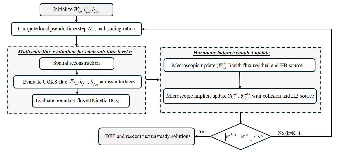
Overall, the proposed HB-UGKS framework inherently incorporates three distinct time scales. The first is the macroscopic physical period $T$, represented by $N_{\text{T}}$ collocation points over one period. The second is the local kinetic evolution time $[0,\Delta\Gamma_{f}]$, explicitly utilized during the interface flux evaluation to capture the multiscale characteristics of the flow. The third is the pseudo-time $\Gamma$ for iteration, which relaxes the coupled harmonic balance system toward convergence. While the interface flux evaluation remains strictly localized at each collocation point, the time spectral operator introduces a global temporal coupling across the entire period. For clarity, the overall pseudo-time marching procedure is illustrated in Fig. 1.

Figure 1: Flowchart of the pseudo-time marching procedure for the HB-UGKS solver.

3 Results and discussion

In this section, the HB-UGKS is assessed for two representative oscillatory cavity problems. The shear-driven case is used to verify the linear response, the high-frequency limit, and the continuum limit, while the thermally driven case is employed to examine the nonlinear behaviors under finite-amplitude excitations. Across these two cases, both the efficiency and accuracy of the HB-UGKS framework are evaluated and compared to provide a comprehensive demonstration of its practical potential.

3.1 Shear-driven oscillatory cavity flow

3.1.1 Numerical setup

The two-dimensional shear-driven oscillatory cavity flow serves as a standard benchmark for verifying unsteady kinetic solvers. The computational domain is a rectangular cavity defined by $(x,y)\in[0,L]\times[0,H]$, with an aspect ratio of $A=L/H$. The bottom, left, and right walls are stationary and maintained at a constant reference temperature $T_{0}$. The flow is driven by the top lid ($y=H$), which oscillates harmonically in its own plane with a prescribed velocity:

$$U_{w}(t)=\overline{U}_{w}+U_{a}\cos(\omega t)$$ (34)

$$V_{w}(t)=0$$ (35)

where $\overline{U}_{w}$ denotes the time-averaged horizontal velocity of the lid, and $U_{a}$ is the oscillation amplitude. In the present simulations, the time-averaged horizontal velocity of lid is set to zero ($\overline{U}_{w}=0$), and a sufficiently small oscillation amplitude of $U_{a}=0.0015\sqrt{2RT_{0}}$ is adopted to ensure the flow closely approximates the linear regime. This configuration is consistent with the linearized Boltzmann equation framework proposed by Wu et al. [35].

The flow regime is governed by two fundamental dimensionless parameters. The Knudsen number (Kn), defined based on the cavity height $H$, is expressed as:

$$Kn=\frac{\lambda_{mfp}}{H}=\frac{4\alpha(5-2\omega_{VSS})(7-2\omega_{VSS})}{5(\alpha+1)(\alpha+2)}\frac{\mu(T_{0})}{\rho_{0}H\sqrt{2\pi RT_{0}}}$$ (36)

where $\lambda_{mfp}$ is the molecular mean free path, $\rho_{0}$ is the initial uniform density, and $\mu(T_{0})$ is the reference dynamic viscosity. To accurately model Argon gas, the Variable Soft Sphere (VSS) collision model is employed. The dynamic viscosity follows a standard power-law temperature dependence with an index of $\omega_{VSS}=0.81$ and an angular scattering parameter of $\alpha=1.0$. The Strouhal number (St), which characterizes the oscillation frequency, is defined as:

$$St=\frac{\omega H}{\sqrt{2RT_{0}}}$$ (37)

For the standard square cavity ($A=1$), the physical space is discretized using a $90\times 90$ non-uniform structured mesh. To accurately resolve the near-wall multiscale gradients and Knudsen layer effects, the mesh is progressively refined towards all physical boundaries with a minimum grid spacing of $\Delta s_{\min}=0.001H$ adjacent to the walls. For cavities with different aspect ratios, the number of cells in the horizontal direction is scaled proportionally while maintaining the identical vertical resolution: $N_{x}=180$ for $A=2$, and $N_{x}=45$ for $A=0.5$.

In the velocity space, the continuous microscopic velocity is truncated at $[-4,4]^{2}$ (normalized by $\sqrt{2RT_{0}}$). A regime-dependent discretization strategy is adopted to balance accuracy and computational efficiency. For the near-continuum and slip regimes ($Kn\leq 0.1$), a $28\times 28$ Gauss-Hermite quadrature is employed, whereas a $64\times 64$ Newton-Cotes rule is utilized for the highly rarefied regimes ($Kn\geq 1.0$). In these standard cases, the reference viscosity $\mu(T_{0})$ is explicitly dictated by the prescribed Knudsen number via Eq. (36). Conversely, for the specific continuum limit cases (detailed in Section 3.1.3), a $16\times 16$ uniform discrete velocity grid is sufficient, and the reference viscosity is instead determined by the macroscopic Reynolds number as:

$$\mu(T_{0})=\frac{\rho_{0}\overline{U}_{w}H}{Re}$$ (38)

As described previously, the conservative macroscopic variables at each sub-time level $n$ are directly obtained from the velocity-space moments of the distribution function $h_{n}$. Furthermore, the local shear stress, which is essential for characterizing the aerodynamic viscous response, can be evaluated as:

$$\tau_{xy,n}=\sum_{\alpha}w_{\alpha}(u_{\alpha}-U_{n})(v_{\alpha}-V_{n})h_{n}$$ (39)

Once the pseudo-time marching of the HB-UGKS converges, the periodic steady-state solutions (including both macroscopic variables and microscopic distribution functions) at the $N_{\text{T}}$ collocation points are obtained. Subsequently, a discrete Fourier transform is applied as a post-processing step to extract the Fourier coefficients for each variable. The $k$-th order complex Fourier coefficient $\widehat{q}_{k}(\mathbf{x})$ is defined as:

$$\widehat{q}_{k}(\mathbf{x})=\frac{1}{N_{\text{T}}}\sum_{n=0}^{N_{\text{T}}-1}q_{n}(\mathbf{x}),e^{-ik\omega t_{n}}$$ (40)

where $q_{n}(\mathbf{x})$ represents any variable of interest at the $n$-th sub-time level. Specifically, the zeroth-order coefficient ($k=0$) yields the time-averaged flow field, the first-order coefficient ($k=1$) represents the complex amplitude of the fundamental harmonic, and components with $k>1$ capture the higher-order harmonics associated with nonlinear flow responses. For the aerodynamic analysis of the oscillatory lid, we apply this transformation directly to the horizontal velocity $U$ and the local shear stress $\tau_{xy}$ to obtain their first-order complex amplitudes, denoted as $\widehat{U}_{1}(\mathbf{x})$ and $\widehat{\tau}_{xy,1}(\mathbf{x})$

3.1.2 High-frequency behavior and gas anti-resonance phenomenon

A harmonic independence study at $Kn=0.1$ and $St=2$ confirms that $N_{\text{H}}=1$ is sufficient for flows within the near-linear regime. Figure 2 compares the real and imaginary components of the normalized fundamental velocity amplitude, $\widehat{U}_{1}/U_{a}$, along the vertical centerline for $N_{\text{H}}=1$ and $N_{\text{H}}=2$. The two solutions are visually indistinguishable, confirming that the fundamental harmonic completely dominates the dynamic response and that $N_{\text{H}}=1$ provides adequate accuracy for all subsequent weakly excited cases.

Figure 2: Harmonic independence verification: $\Re(\widehat{U}_{1}/U_{a})$ and $\Im(\widehat{U}_{1}/U_{a})$ along $x=0.5L$ for $N_{\text{H}}=1$ and $N_{\text{H}}=2$ ($Kn=0.1$, $St=2$).

To quantitatively evaluate the overall aerodynamic response on the oscillating lid, the spatially averaged fundamental amplitudes of the horizontal velocity and shear stress are normalized as follows:

$$\widetilde{U}=\frac{\big|\langle\widehat{U}_{1}\rangle_{\text{wall}}\big|}{U_{a}}$$ (41)

$$\widetilde{\tau}_{xy}=\frac{\big|\langle\widehat{\tau}_{xy,1}\rangle_{\text{wall}}\big|}{p_{0}U_{a}/\sqrt{2RT_{0}}}$$ (42)

where $\langle\cdot\rangle_{\text{wall}}$ denotes the spatial average along the top boundary of length $L$. To strictly account for the non-uniform mesh distribution, this spatial average is numerically evaluated as a discrete integral weighted by the local cell width, i.e., $\langle q\rangle_{\text{wall}}=\frac{1}{L}\sum_{i=1}^{N_{x}}q_{i}\Delta x_{i}$, with $\Delta x_{i}$ being the horizontal dimension of the $i$-th cell adjacent to the lid.

The numerical framework is further examined in the high-frequency limit at $St=30$. In this regime, the oscillation period is significantly shorter than the local mean molecular collision time, effectively driving the near-wall gas behavior into a dynamically collisionless state, despite the nominal Knudsen number of $Kn=0.1$. Figure 3 displays the local distributions of $\widetilde{U}$ and $\widetilde{\tau}_{xy}$ along the oscillating lid for three aspect ratios. Away from the cavity corners, both normalized amplitudes exhibit nearly uniform profiles. This uniformity arises because the extremely short forcing period prohibits any meaningful intermolecular collisions or acoustic wave propagation from laterally redistributing the momentum.

Consequently, the macroscopic state of the gas adjacent to the lid is entirely determined by the instantaneous gas-surface interaction. Based on kinetic theory, the local velocity distribution function near the wall degenerates into a superposition of an unperturbed half-Maxwellian incident from the bulk and a fully accommodated half-Maxwellian reflected from the wall. This half-space molecular velocity integration theoretically yields a macroscopic gas velocity exactly half that of the wall ($\widetilde{U}\to 0.5$), and a normalized wall shear stress governed by the transverse thermal flux ($\widetilde{\tau}_{xy}\to 1/\sqrt{\pi}$). The HB-UGKS precisely recovers these theoretical collisionless limits, with spatially averaged relative deviations bounded tightly within $2\%$.

(a) $\widetilde{U}$ along the oscillating lid

(b) $\widetilde{\tau}_{xy}$ along the oscillating lid

Figure 3: Normalized fundamental amplitudes along the top lid at $St=30$, $Kn=0.1$ for different aspect ratios. Dashed lines: exact collisionless limits.

Figure 4 presents the evolution of $\widetilde{U}$ and $\widetilde{\tau}_{xy}$ across a wide range of Strouhal numbers for $Kn=0.1$. The solutions of the HB-UGKS demonstrate excellent agreement with the linearized Boltzmann solutions of Wu et al. [35] across the entire tested frequency spectrum. Notably, the wall shear stress exhibits a non-monotonic trend, developing a distinct local minimum that corresponds to the gas anti-resonance phenomenon. Physically, this minimum stems from the destructive interference between the viscous waves generated by the oscillating lid and the secondary waves reflected from the stationary boundaries. Because the lateral travel distance determines the phase condition for this interference, the resonant minimum systematically shifts with the cavity aspect ratio. Finally, as $St$ approaches infinity, both amplitudes asymptotically converge to their respective collisionless limits.

(a) $\widetilde{U}$ vs $St$

(b) $\widetilde{\tau}_{xy}$ vs $St$

Figure 4: Spatially averaged normalized amplitudes vs $St$ for $Kn=0.1$ and different aspect ratios. Symbols: HB-UGKS; lines: reference [35].

3.1.3 Multiscale flow structures and continuum limit verification

The phase-resolved density fields offer direct insight into the internal transport mechanisms. Figure 5 illustrates the normalized density variations along the top lid at $Kn=0.1$ for different Strouhal numbers. At low frequencies ($St=2$ and $4$), the acoustic disturbances propagate throughout the entire cavity, resulting in relatively smooth phase variations. However, at the intermediate frequency ($St=12$), the density response becomes increasingly localized near the upper corners. At the highest frequency ($St=30$), these fluctuations are confined to a very thin layer. As evidenced by the rapid spatial decay and the emergence of multiple zero-crossings within the near-wall region ($X/H<0.05$) in Fig. 5(d), the density fluctuations at $St=30$ are highly localized, characterized by a much more pronounced phase lag compared to the lower frequency cases. This evolution represents a clear transition from a bulk-scale acoustic response to a boundary-confined high-frequency regime, where the wave propagation speed limits the extent of the disturbance.

(a) $St=2$

(b) $St=4$

(c) $St=12$

(d) $St=30$

Figure 5: Normalized density variation $(\rho_{n}-\rho_{0})/(\rho_{0}U_{a})$ along the top lid at different phase angles for $Kn=0.1$, $A=0.5$.

Figure 6 shows the fundamental harmonic amplitudes for a square cavity at $Kn=0.1$. The vertical profile of the normalized fundamental velocity amplitude illustrates the penetration depth of the oscillatory momentum. At low $St$, viscous diffusion allows momentum to reach the lower regions of the cavity. At high $St$, the oscillation is restricted to a narrow region near the lid, exhibiting a typical Stokes-layer structure. Correspondingly, the normalized fundamental amplitude of the wall shear stress displays a U-shaped distribution. The sharp amplification at the corners is caused by the interaction of two-dimensional waves. As $St$ increases, the wall stress becomes more uniform, gradually approaching the collisionless limit discussed previously.

(a) $|\widehat{U}_{1}|/U_{a}$ along $x=0.5L$

(b) $|\widehat{\tau}_{xy,1}|/\tau_{\text{ref}}$ along $y=H$

Figure 6: Normalized fundamental harmonic amplitudes of horizontal velocity and shear stress at $Kn=0.1$, $A=1$ for different Strouhal numbers.

The results for $Kn=1.0$ (Figure 7) highlight the influence of rarefaction. Compared to the $Kn=0.1$ case, the velocity slip at the wall is much larger, and the momentum penetration into the cavity is further reduced. These features reflect the weakened collisional coupling between gas molecules, which shifts the physical mechanism from viscous diffusion toward particle free transport.

(a) $|\widehat{U}_{1}|/U_{a}$ along $x=0.5L$

(b) $|\widehat{\tau}_{xy,1}|/\tau_{\text{ref}}$ along $y=H$

Figure 7: Normalized fundamental harmonic amplitudes of horizontal velocity and shear stress at $Kn=1.0$, $A=1$ for different Strouhal numbers.

While the comprehensive all-$Kn$ profiles are omitted for brevity, a consistent trend is observed across the tested Knudsen numbers at $St=2$ and $A=1$. The flow structure evolves from a near-continuum Stokes layer with negligible velocity slip to a highly rarefied response characterized by pronounced wall slip. Concurrently, the variation in wall shear stress becomes progressively weaker, reflecting the diminishing role of viscous diffusion and the increasing dominance of particle free transport.

Figure 8 illustrates the fundamental harmonic amplitudes of the normalized horizontal velocity along the centerline and the corresponding wall shear stress. At the near-continuum regime of $Kn=0.01$, the velocity profile exhibits a classic Stokes-layer structure characterized by a spatial velocity reversal near the lid ($Y/H\approx 0.8\sim 0.95$), reflecting strong viscous wave interactions with the wall. In this regime, the wall slip is negligible, and momentum penetrates deeply through viscous diffusion driven by the low frequency. Correspondingly, the wall shear stress profile is strongly U-shaped, featuring sharp amplifications at the cavity corners ($X/L=0$ and $X/L=1$) due to the interference between the primary lid-driven viscous waves and wall reflections. As $Kn$ increases, these continuum phenomena are suppressed. The spatial oscillation in the velocity field vanishes, and the slip velocity at the moving wall becomes progressively more pronounced. At the highly rarefied limit of $Kn=10$, the velocity profile degenerates into a near-linear, shear-layer-like distribution with massive slip. Concurrently, the effective momentum penetration depth is substantially reduced; the weakened collisional coupling restricts momentum transfer into the cavity interior, confining the disturbance near the driven lid. This rarefaction effect is equally evident in the wall shear stress, where the initial U-shaped distribution is rapidly flattened. At $Kn=10$, the wall stress becomes virtually uniform with negligible corner enhancement.

(a) Normalized velocity amplitude $|\widehat{U}_{1}|/U_{a}$ along $x=0.5L$

(b) Normalized amplitude of wall shear stress $|\widehat{\tau}_{xy,1}|/\tau_{\text{ref}}$ along $y=H$

Figure 8: All-$Kn$ evolution of fundamental harmonic amplitudes at $St=2,A=1$ for different Knudsen numbers.

Finally, to demonstrate that the HB-UGKS inherits the multiscale asymptotic preserving (AP) property of the standard UGKS, it is essential to verify its capability to recover macroscopic hydrodynamic behaviors in the continuum limit. Although the Harmonic Balance method is inherently formulated for unsteady periodic flows, it provides an elegant pathway for this steady-state verification. Specifically, the cavity is driven by a time-averaged lid velocity $\overline{U}_{w}=0.15$ superimposed with a small oscillation amplitude $U_{a}=0.0015$ (1% of the time-averaged). The reference viscosity is calculated from Eq. 38, and two standard Reynolds numbers are considered: $Re=100$ and $Re=1000$.

Given the exceedingly small amplitude of the oscillation, its nonlinear impact on the background flow is negligible. Consequently, the time-averaged flow field—represented directly by the zeroth-order harmonic component—is practically equivalent to the pure steady-state solution. Figure 9 compares these computed time-averaged centerline velocities against the classic benchmark data of Ghia et al. [14]. The excellent agreement for both Reynolds numbers confirms that the multiscale flux within the present framework degenerates to the NS equations in the continuum limit.

(a) $Re=100$

(b) $Re=1000$

Figure 9: Continuum limit: $\widehat{U}_{0}/\overline{U}_{w}$ and $\widehat{V}_{0}/\overline{U}_{w}$ along the centerlines compared with the benchmark data of Ghia et al.

3.1.4 Evaluation of computational efficiency of the HB-UGKS

The harmonic balance equation system is formulated not only to obtain the periodic solution accurately but also to significantly reduce the computational cost. To ensure a rigorous and fair comparison, both the calculations of the HB-UGKS and the time-domain UGKS based on time-marching strategy are executed within the same code framework on an identical high-performance computing (HPC) platform. They share identical spatial meshes, discrete velocity spaces, spatial reconstruction schemes, explicit flux evaluation methods, boundary conditions, and a parallelization setting. The fundamental distinction lies solely in the treatment of the temporal derivative: while the time-domain method advances explicitly step-by-step in physical time, the HB-UGKS transforms the temporal derivative into a spectral source term, which necessitates a coupled iterative loop over all sub-time levels in pseudo-time. For a conservative variable $W^{(p)}\in\{\rho,\rho U,\rho V,\rho E\}$, the residuals used to evaluate the convergence to the periodic steady state are defined as:

$$\mathcal{R}_{\mathrm{HB}}^{(p)}(k) =\left[\frac{1}{N_{c}}\sum_{i=1}^{N_{c}}\left(W_{i,0}^{(p),k+1}-W_{i,0}^{(p),k}\right)^{2}\right]^{1/2},$$ (43)

$$\mathcal{R}_{\mathrm{TD}}^{(p)}(n) =\left[\frac{1}{N_{c}}\sum_{i=1}^{N_{c}}\left(W_{i}^{(p)}(nT)-W_{i}^{(p)}((n-1)T)\right)^{2}\right]^{1/2},$$

where $N_{c}$ is the total number of spatial control volumes. For the HB-UGKS, the residual measures the pseudo-time convergence specifically at the beginning of the period ($t_{0}=0$). To ensure a strict correspondence, the residual for the time-domain (TD) method evaluates the difference at the exact same phase across consecutive physical periods (i.e., between $t=nT$ and $t=(n-1)T$). Analogous definitions apply to all other conservative variables. For a clear visual comparison, the convergence curves are plotted using the shifted density-residual reduction, $\Delta r_{\rho}=\log_{10}\mathcal{R}_{\rho}-\log_{10}\mathcal{R}_{\rho,1}$, and the shifted wall-clock time, $\Delta t_{\mathrm{wall}}=t_{\mathrm{wall}}-t_{\mathrm{wall},1}$, where the subscript 1 denotes the first valid residual data point of the respective method.

Figure 10 compares the wall-clock time required for the density residual to decrease by seven orders of magnitude at two representative Strouhal numbers. At $St=2$, the advantage of the HB-UGKS is positive but moderate, yielding a speedup factor of approximately $1.4\times$. In this low-frequency regime, the forcing period is relatively long. The physical time required for the flow field to reach a stable periodic state is covered within merely a few forcing cycles. Because the explicit time-marching strategy only needs to simulate a small number of periods to achieve convergence, its computational cost remains acceptable.

Figure 10: Convergence comparison between HB-UGKS and explicit time-domain UGKS for the shear-driven cavity under the unified benchmark definition of Eq. (43). The ordinate is the shifted density-residual reduction $\Delta r_{\rho}$, and the abscissa is the shifted wall-clock time $\Delta t_{\mathrm{wall}}$.

At $St=30$, the speedup surges to about $9.2\times$. This dramatic difference highlights the inherent limitation of time-domain marching for high-frequency flows. The absolute physical time required for the internal flow to stabilize remains roughly constant, independent of the driving frequency. However, because the single forcing period at $St=30$ is extremely short, the explicit TD method is forced to march through dozens of cycles (often exceeding 50 periods) just to accumulate enough physical time to reach the stable periodic state. Simulating such a large number of cycles makes the time-domain approach highly inefficient. The HB formulation fundamentally circumvents this limitation. Instead of marching forward in physical time, the HB method transforms the unsteady problem into a set of coupled steady-state equations. This allows it to directly compute the final periodic state, completely avoiding the slow period-by-period settling process.

3.2 Large-Amplitude Thermally Driven Oscillatory Cavity Flow

The second case investigates a thermally driven oscillatory flow within a square cavity ($A=1$). In contrast to the preceding small-amplitude shear-driven case, this configuration is specifically designed to examine finite-amplitude nonlinear effects. The bottom, left and right walls are maintained at a constant reference temperature $T_{0}$. The top-wall temperature undergoes a periodic oscillation, given by

$$T_{w}(t)=T_{0}+T_{a}\cos(\omega t),$$ (44)

where the temperature amplitude is set to a significantly large value of $T_{a}=0.3T_{0}$, and $\omega$ is the angular frequency determined by the Strouhal number.

This substantial thermal forcing continuously drives the gas away from local thermodynamic equilibrium and triggers pronounced higher-order harmonic responses. It therefore provides a rigorous test for both the non-equilibrium kinetic transport and the nonlinear harmonic coupling within the HB-UGKS framework. To ensure numerical consistency, the spatial domain is discretized using the identical mesh from the preceding shear-driven case. Furthermore, the resolution of the discrete velocity space remains unchanged across all tested Knudsen numbers and working conditions. Unless otherwise specified, the phase-resolved validation results in this subsection are presented at $St=2$ across four representative Knudsen numbers ($Kn=0.01,0.1,1.0$, and $10$). Finally, an analysis of the computational convergence efficiency at both low and high frequencies is provided at the end of this subsection.

3.2.1 Harmonic independence verification and multiscale spatial structures

Under finite-amplitude thermal forcing, the flow response is no longer dominated by the fundamental frequency alone. The substantial temperature variation ($T_{a}=0.3T_{0}$) at the boundary induces strong nonlinearities within both the gas-kinetic collision operator and the convective macroscopic fluxes. This nonlinearity acts as a mechanism for cross-frequency energy transfer, generating pronounced higher-order harmonics. Figure 11 demonstrates this by comparing the vertical-velocity profiles at $t=0.5T$ truncated at $N_{\text{H}}=1$, $2$, and $3$. The condition of $N_{\text{H}}=1$ severely under-predicts the peak response because it fails to capture the nonlinear transfer of energy to higher frequencies. In contrast, the solutions for $N_{\text{H}}=2$ and $N_{\text{H}}=3$ are virtually identical, confirming that the second-order harmonic is essential and sufficient to resolve the leading-order nonlinearities in the present configuration. Consequently, all subsequent thermally driven simulations employ $N_{\text{H}}=2$.

Figure 11: Harmonic independence verification: spatial distribution of the vertical velocity $V$ at $t=0.5T$ calculated with $N_{\text{H}}=1,2,$ and $3$.

Once the required number of harmonics is determined, the non-equilibrium thermodynamic features of the transitional flow are investigated. Figure 12 presents the temperature distribution along the vertical centerline at four distinct phase angles for $Kn=0.1$.

Figure 12: Dynamic temperature profiles along the vertical centerline ($x=0.5L$) at different phase angles within one oscillation period ($Kn=0.1$). Markers denote the reference data of Yang et al. [41].

These profiles reveal several key physical phenomena intrinsic to this regime. Most notably, a pronounced temperature jump is evident adjacent to the oscillating top wall. Although the physical wall temperature reaches extreme values of $1.3T_{0}$ and $0.7T_{0}$ at $t=0$ and $t=0.5T$, respectively, the adjacent gas temperature only reaches approximately $1.17T_{0}$ and $0.79T_{0}$. This substantial macroscopic temperature slip is a direct manifestation of the Knudsen layer effect. Accompanying this boundary phenomenon is the clear spatial attenuation of the periodic thermal wave. As the thermal disturbance propagates downward, its energy is heavily dissipated by intermolecular collisions within the upper portion of the cavity. Consequently, the temperature variation decays rapidly along the vertical axis, leaving the gas near the stationary bottom wall largely undisturbed and anchored at the reference temperature ($T/T_{0}\approx 1.0$). Beyond these spatial characteristics, the profiles also capture the temporal phase lag induced by finite-rate thermal diffusion. For instance, at $t=0.25T$ (the blue curve), while the top-wall temperature has already reverted to $1.0T_{0}$, the thermal energy injected during the preceding heating phase continues to penetrate inward, resulting in an elevated temperature distribution in the cavity core ($Y/H\approx 0.6\sim 0.9$). To definitively assess the spatial accuracy and multiscale capability of the present framework, these reconstructed flow fields are compared against the reference mesoscopic data of Yang et al. [41]. The results of the HB-UGKS exhibit excellent agreement with the reference data throughout the entire domain, proving its ability to precisely capture the dynamic thermal fluctuations, and the Knudsen layer slip.

The spatial penetration of the oscillatory momentum across different flow regimes is clearly illustrated by the vertical velocity profiles along the centerline (Figure 13). At the near-continuum limit ($Kn=0.01$), the dynamic response is heavily damped by intermolecular collisions, tightly confining the macroscopic motion to the upper portion of the cavity. As rarefaction increases to the slip regime ($Kn=0.1$), the thermal wave penetrates much deeper into the core. However, the momentum transfer remains collision-dominated, exhibiting distinct spatial wave-like structures and phase lags along the vertical direction. A different flow behavior emerges under highly rarefied conditions ($Kn=1.0$ and $10$). Because the intermolecular collision frequency becomes extremely low, particles heated by the top wall can travel directly across the cavity with very few collisions. Consequently, the local wave propagation is replaced by a unified expansion and contraction of the entire gas. This transition clearly demonstrates the physical shift from diffusion-dominated thermal penetration to collisionless particle free transport. The excellent agreement between the HB-UGKS results and the reference data across all regimes robustly verifies the sufficient accuracy of the present framework.

(a) $Kn=0.01$

(b) $Kn=0.1$

(c) $Kn=1.0$

(d) $Kn=10$

Figure 13: Vertical velocity ($V$) profiles along the cavity centerline ($x=0.5L$) at different phase angles for various Knudsen numbers. Markers denote the reference data of Yang et al. [41].

3.2.2 Phase-Dependent Flow Structures and Nonlinear Temporal Asymmetry

In addition to changing the time-averaged spatial penetration, the large-amplitude thermal forcing also affects the dynamic structure and temporal behavior of the flow. To illustrate this, Figure 14 displays the phase-resolved contours of the vertical velocity at two opposing phases: $t/T=0.25$ (the heating/expansion phase) and $t/T=0.75$ (the cooling/relaxation phase). At $Kn=0.1$, the velocity field remains localized near the top wall in both plots, with similar magnitudes and opposite directions. This behavior resembles a symmetric, diffusion-damped wave. However, at $Kn=10$, the vertical velocity contours fill a much larger portion of the cavity. Moreover, there is a clear asymmetry between the results at $t/T=0.25$ and $t/T=0.75$. The magnitude and vertical distribution of the velocity do not perfectly match across the opposing phases, pointing towards a breakdown of dynamic equivalence.

(a) $Kn=0.1,\;t/T=0.25$

(b) $Kn=0.1,\;t/T=0.75$

(c) $Kn=10,\;t/T=0.25$

(d) $Kn=10,\;t/T=0.75$

Figure 14: Phase-resolved contours of the vertical velocity $V$ in the thermally driven cavity at Knudsen number 0.1 and 10.

The reconstructed time history of the flow variables (Figure 15) provides a clear view of the dynamic differences across flow regimes. For the temperature response (Figure 15a), the oscillation amplitude increases as the gas becomes more rarefied. Despite these variations in amplitude and phase, the temperature waveforms remain largely sinusoidal across all regimes, without obvious shape distortion.

Conversely, the vertical velocity (Figure 15b) reveals an opposite trend in amplitude. At the near-continuum limit ($Kn=0.01$), the velocity fluctuation is relatively strong. Similar to the temperature response, the velocity waveform remains largely sinusoidal, but it exhibits an asymmetry around the zero-velocity axis, where the positive peak reaches a higher absolute magnitude than the negative trough. As the flow becomes highly rarefied ($Kn=1.0$ and $10$), the overall velocity amplitude decreases. This contrasting amplitude behavior reflects the fundamental transition in momentum transport. At low Knudsen numbers, the collective collisions among gas molecules effectively transmit the boundary oscillation into the bulk fluid; in the free-molecular limit, this collective interaction weakens, leading to a diminished macroscopic velocity response. The ability of the HB-UGKS to accurately capture these distinct amplitude and mean-shift trends across different flow regimes demonstrates its reliable numerical fidelity.

(a) Temperature time history

(b) Vertical velocity time history

Figure 15: Temporal evolution of temperature and vertical velocity at the probe point ($X=0.5L,Y=0.9H$) reconstructed over two oscillation periods.

3.2.3 Convergence Efficiency and Accuracy Verification

The computational efficiency of the proposed HB-UGKS is further evaluated in the thermally driven cavity and compared against the time-domain (TD) marching method within an identical underlying numerical framework. To ensure a rigorous and consistent comparison with the preceding shear-driven case, both solvers are executed until the macroscopic density residual strictly drops by seven orders of magnitude, following the exact same benchmark criteria outlined in Eq. (43). Furthermore, quantitative assessments confirm that the relative difference in the final reconstructed flow fields between the two approaches remains consistently below $0.3\%$ across all tested working conditions. This verifies that the HB formulation accurately preserves the physical fidelity of the TD method without introducing additional truncation errors.

With the numerical accuracy confirmed, Figure 16 compares the wall-clock time required for deep convergence at two representative frequencies.

Figure 16: Convergence comparison between HB-UGKS and explicit time-domain UGKS for the thermally driven cavity under the unified benchmark definition of Eq. (43). The ordinate is the shifted density-residual reduction $\Delta r_{\rho}$, and the abscissa is the shifted wall-clock time $\Delta t_{\mathrm{wall}}$.

Similar to the observations in the shear-driven problem, the efficiency gain is highly frequency-dependent. At the low-frequency condition ($St=2$), the speedup is marginal, standing at approximately $1.06\times$. Compared to the $1.4\times$ speedup achieved in the shear-driven case at the same $St$, this reduction in relative efficiency stems directly from the increased harmonic count. Because the finite-amplitude thermal forcing excites strong nonlinearities, the present case requires $N_{\text{H}}=2$ rather than $N_{\text{H}}=1$. This implies a larger number of sampling sub-time levels ($2N_{\text{H}}+1$) and a substantially expanded, strongly coupled nonlinear algebraic system. The augmented memory footprint and the heavier arithmetic operations required to invert this coupled matrix severely compromise the baseline speedup. Meanwhile, the explicit TD solver remains competitive at this low frequency since it only needs to march through a small number of long oscillation periods before reaching a stable state, largely offsetting the algorithmic advantage of the HB formulation.

As the driving frequency increases to $St=30$, however, the computational bottleneck shifts dramatically, and the HB-UGKS solver achieves a pronounced speedup of approximately $8.33\times$. The fundamental physical reason is similar to that of the previous shear-driven case: the physical relaxation time of the cavity flow is an intrinsic property independent of the wall oscillation frequency. When the period becomes exceedingly short, the TD method is trapped in an inefficient transient march, requiring scores of cycles to accumulate enough physical time to reach the periodic state. The HB method inherently bypasses this period-by-period settling phase. By directly solving for the periodic steady state in the time domain, its computational cost remains insensitive to the length of the physical period, demonstrating its significant advantage and robustness for simulating high-frequency, non-equilibrium oscillatory flows.

4 Conclusions

In this work, a time-domain harmonic balance unified gas-kinetic scheme (HB-UGKS) is developed and applied to the analysis of temporally periodic flows across all Knudsen regimes. The proposed method employs a spectral approach to treat the time derivative terms in both the microscopic and macroscopic governing equations. Simultaneously, the UGKS is utilized to evaluate interfacial fluxes, thereby ensuring accurate multiscale transport across different flow regimes. By transforming the original unsteady equation system into a block-coupled, quasi-steady system, the periodic flow field is efficiently resolved through explicit pseudo-time marching combined with local time-stepping.

For the shear-driven oscillatory cavity under small-amplitude excitation, the method confirms harmonic independence. It accurately recovers both the continuum Navier–Stokes limit and the high-frequency collisionless limit, while precisely capturing the geometric anti-resonance phenomenon. In the case of the large-amplitude thermally driven cavity, the scheme captures phase-resolved macroscopic fields over a wide range of Knudsen numbers. Furthermore, it successfully resolves the non-sinusoidal waveform distortions associated with unequal heating and cooling relaxation mechanisms in rarefied flows.

A rigorous convergence comparison with the standard time-domain UGKS demonstrates that the HB formulation provides a substantial computational advantage across the tested frequency range, all while maintaining a relative discrepancy of less than $0.3\%$ in the final reconstructed flow fields. Under a strict seven-order-of-magnitude residual reduction target, the shear-driven cavity yields a speedup factor of approximately $1.4\times$ at $St=2$ and $9.0\times$ at $St=30$. For the thermally driven cavity, the corresponding speedup factors are $1.06\times$ at $St=2$ and $8.26\times$ at $St=30$. Consequently, while the efficiency gain is case-dependent, it remains consistently positive and becomes significantly more pronounced as the forcing frequency increases.

Overall, the present results demonstrate that the HB-UGKS is a robust and highly efficient framework for multiscale periodic gas-kinetic simulations. It strictly preserves the physical fidelity of the UGKS while substantially reducing the computational cost required to reach a periodic steady state. This establishes a rigorous algorithmic foundation for future implicit harmonic balance solvers and complex multidimensional, multi-frequency oscillatory flow applications.

References

- [1] (1999) Report: a model for flows in channels, pipes, and ducts at micro and nano scales. Microscale Thermophysical Engineering 3 (1), pp. 43–77. External Links: Document Cited by: §1.
- [2] (1954) A model for collision processes in gases. i. small amplitude processes in charged and neutral one-component systems. Physical review 94 (3), pp. 511. Cited by: §1, §2.1.
- [3] (1963) Approach to translational equilibrium in a rigid sphere gas. Phys. fluids 6, pp. 1518–1519. Cited by: §1.
- [4] (1970) Direct simulation and the boltzmann equation. Physics of Fluids 13 (11), pp. 2676–2681. Cited by: §1.
- [5] (1994) Molecular gas dynamics and the direct simulation of gas flows. Oxford university press. Cited by: §1.
- [6] (1964) Study of rarefied shear flow by the discrete velocity method. Journal of Fluid Mechanics 19 (3), pp. 401–414. External Links: Document Cited by: §1.
- [7] (2010) Numerical regularized moment method of arbitrary order for boltzmann-bgk equation. SIAM Journal on Scientific Computing 32 (5), pp. 2875–2907. External Links: Document Cited by: §1.
- [8] (2000) Rarefied gas dynamics: from basic concepts to actual calculations. Vol. 21, Cambridge university press. Cited by: §1.
- [9] (2015) A comparative study of an asymptotic preserving scheme and unified gas-kinetic scheme in continuum flow limit. Journal of computational physics 288 (), pp. 52–65. External Links: Document Cited by: §2.3.
- [10] (1965) Kinetic-theoretic description of the formation of a shock wave. The Physics of Fluids 8 (1), pp. 12–22. Cited by: §1.
- [11] (2000) A time-linearized navier–stokes analysis of stall flutter. J. Turbomach. 122 (3), pp. 467–476. Cited by: §1.
- [12] (2013-10) Simulating periodic unsteady flows using a cubic-spline-based time collocation method. Journal of Turbomachinery 136 (4), pp. 041014. External Links: ISSN 0889-504X, Document Cited by: §1.
- [13] (2001) Statistical simulation of low-speed rarefied gas flows. Journal of Computational Physics 167 (2), pp. 393–412. External Links: ISSN 0021-9991, Document Cited by: §1.
- [14] (1982) High-re solutions for incompressible flow using the navier-stokes equations and a multigrid method. Journal of computational physics 48 (3), pp. 387–411. Cited by: §3.1.3.
- [15] (2021) Progress of discrete unified gas-kinetic scheme for multiscale flows. Advances in Aerodynamics 3 (1), pp. 6. Cited by: §1.
- [16] (2005-10) Oscillatory shear-driven gas flows in the transition and free-molecular-flow regimes. Physics of Fluids 17 (10), pp. 100611. External Links: ISSN 1070-6631, Document Cited by: §1.
- [17] (2006-11) The limits of navier-stokes theory and kinetic extensions for describing small-scale gaseous hydrodynamics. Physics of Fluids 18 (11), pp. 111301. External Links: ISSN 1070-6631, Document Cited by: §1.
- [18] (1993) Linearized euler predictions of unsteady aerodynamic loads in cascades. AIAA journal 31 (3), pp. 540–550. Cited by: §1.
- [19] (2013) Harmonic balance methods applied to computational fluid dynamics problems. International Journal of Computational Fluid Dynamics 27 (2), pp. 52–67. Cited by: §1.
- [20] (2002) Computation of unsteady nonlinear flows in cascades using a harmonic balance technique. AIAA journal 40 (5), pp. 879–886. Cited by: §1.
- [21] (1998) MICRO-electro-mechanical-systems (mems) and fluid flows. Annual Review of Fluid Mechanics 30 (Volume 30, 1998), pp. 579–612. External Links: ISSN 1545-4479 Cited by: §1.
- [22] (2007) A low-variance deviational simulation monte carlo for the boltzmann equation. Journal of Computational Physics 226 (2), pp. 2341–2358. External Links: ISSN 0021-9991, Document Cited by: §1.
- [23] (2012) A unified gas-kinetic scheme for continuum and rarefied flows ii: multi-dimensional cases. Communications in Computational Physics 12 (3), pp. 662–690. Cited by: §1.
- [24] (2019) Time-space spectral method for rotor–rotor/stator–stator interactions. Journal of Turbomachinery 141 (11), pp. 111006. Cited by: §1.
- [25] (2018) Implicit solution of harmonic balance equation system using the lu-sgs method and one-step jacobi/gauss-seidel iteration. International Journal of Computational Fluid Dynamics 32 (4-5), pp. 218–232. Cited by: §1.
- [26] (1978) Acoustic streaming. Journal of Sound and Vibration 61 (3), pp. 391–418. External Links: ISSN 0022-460X, Document Cited by: §1.
- [27] (2005) List of symbols. In Computational Fluid Dynamics: Principles and Applications (Second Edition), J. Blazek (Ed.), pp. xiii–xvii. External Links: ISBN 978-0-08-044506-9, Document Cited by: §1.
- [28] (2019) A unified gas-kinetic scheme for continuum and rarefied flows vi: dilute disperse gas-particle multiphase system. Journal of Computational Physics 386, pp. 264–295. External Links: ISSN 0021-9991, Document Cited by: §1.
- [29] (2017-11) A unified gas-kinetic scheme for continuum and rarefied flows v: multiscale and multi-component plasma transport. Communications in Computational Physics 22 (5), pp. 1175–1223. External Links: Document Cited by: §1.
- [30] (2000) Discrete-velocity models and numerical schemes for the boltzmann-bgk equation in plane and axisymmetric geometries. Journal of Computational Physics 162 (2), pp. 429–466. External Links: ISSN 0021-9991, Document Cited by: §1.
- [31] (1968) Generalization of the krook kinetic relaxation equation. Fluid dynamics 3 (5), pp. 95–96. Cited by: §2.1, §2.1.
- [32] (2007) Molecular gas dynamics: theory, techniques, and applications. Springer. Cited by: §1.
- [33] (2015) An asymptotic preserving unified gas kinetic scheme for frequency-dependent radiative transfer equations. Journal of Computational Physics 302, pp. 222–238. External Links: ISSN 0021-9991, Document Cited by: §1.
- [34] (2020) Time implicit unified gas kinetic scheme for 3d multi-group neutron transport simulation. Communications in Computational Physics 28 (3), pp. 1189–1218. Cited by: §1.
- [35] (2014) Oscillatory rarefied gas flow inside rectangular cavities. Journal of Fluid Mechanics 748, pp. 350–367. Cited by: §1, §1, Figure 4, Figure 4, §3.1.1, §3.1.2.
- [36] (2015) A fast spectral method for the boltzmann equation for monatomic gas mixtures. Journal of Computational Physics 298, pp. 602–621. External Links: ISSN 0021-9991, Document Cited by: §1.
- [37] (2019) A fast spectral method for the uehling-uhlenbeck equation for quantum gas mixtures: homogeneous relaxation and transport coefficients. Journal of Computational Physics 399, pp. 108924. External Links: ISSN 0021-9991, Document Cited by: §1.
- [38] (2017) A well-balanced unified gas-kinetic scheme for multiscale flow transport under gravitational field. Journal of Computational Physics 332, pp. 475–491. External Links: ISSN 0021-9991, Document Cited by: §1.
- [39] (2010) A unified gas-kinetic scheme for continuum and rarefied flows. Journal of Computational Physics 229 (20), pp. 7747–7764. Cited by: §1.
- [40] (2022) UGKS-based implicit iterative method for multiscale nonequilibrium flow simulations. SIAM Journal on Scientific Computing 44 (4), pp. B996–B1017. Cited by: §1.
- [41] (2025) Oscillatory thermally driven rarefied flows using a coupled macroscopic/mesoscopic method. Journal of National University of Defense Technology 47 (6), pp. 168–177. Cited by: §1, Figure 12, Figure 12, Figure 13, Figure 13, §3.2.1.
- [42] (2025-07) Numerical stability analysis of implicit solution methods for harmonic balance equations. Journal of Turbomachinery 147 (12), pp. 121010. External Links: ISSN 0889-504X, Document Cited by: §1.
- [43] (2021) General synthetic iterative scheme for nonlinear gas kinetic simulation of multi-scale rarefied gas flows. Journal of Computational Physics 430, pp. 110091. External Links: ISSN 0021-9991, Document Cited by: §1.
- [44] (2017-09) Unified gas-kinetic scheme with multigrid convergence for rarefied flow study. Physics of Fluids 29 (9), pp. 096102. External Links: ISSN 1070-6631, Document Cited by: §1.
- [45] (2019) An implicit unified gas-kinetic scheme for unsteady flow in all knudsen regimes. Journal of Computational Physics 386, pp. 190–217. External Links: ISSN 0021-9991, Document Cited by: §1.
- [46] (2024-10) Investigation of the sigma approximation technique for the solution of the time spectral equation system. Journal of Engineering for Gas Turbines and Power 147 (1), pp. 011027. External Links: ISSN 0742-4795, Document Cited by: §1.