Ghost Degrees of Freedom Without Quantum Runaway: Exact Moment Bounds from an Operator Conservation Law

Abstract

We prove an exact quantum conservation law for a harmonic oscillator coupled to a ghost degree of freedom: a second classical conserved quantity lifts to a quantum operator that commutes with the Hamiltonian with no $\hbar$ corrections, yielding a rigorous, state-independent upper bound on the mean squared phase-space radius for all time and every quantum state with finite initial second moments. The proof uses only canonical commutation relations and the Leibniz rule; it requires no confining potential, no spectral assumptions, and no perturbative expansion. The interaction studied here is bounded and vanishes at large separations, the generic situation in effective field theory, yet this suffices to guarantee quantum stability in the sense of bounded second moments. Three independent numerical frameworks (Heisenberg picture, Schrödinger picture, and Fock-space diagonalization) confirm wavepacket confinement below the analytic bound, a real energy spectrum, and Poisson level statistics numerically consistent with an integrable structure. The absence of a confining potential means the proof is silent on spectral discreteness and the existence of a ground state; those questions, addressed for polynomial confining interactions in concurrent work [12, 11], remain open for the interaction class studied here and represent the sharpest targets for future work. Ghost quantum instability is therefore not an inevitable consequence of a wrong-sign kinetic term but depends critically on the interaction structure.

I Introduction

Ghost fields, degrees of freedom with a wrong-sign kinetic term, appear across a wide range of physically motivated theories: higher-derivative gravity [25], Faddeev-Popov gauge fixing [16], dark-energy models [5], and the Pais-Uhlenbeck oscillator [23]. The Ostrogradsky theorem [22] and standard perturbation theory both suggest that any ghost-containing theory is unstable: the ghost can radiate energy into normal-sector modes without limit, and in quantum field theory the vacuum decay rate naively diverges [6].

Ghost fields arise concretely in the dark energy context. Recent results from the Dark Energy Spectroscopic Instrument (DESI) suggest a dark energy equation-of-state parameter $w<-1$, or a dynamical $w(z)$ crossing the phantom divide [2, 15], at a statistical significance of roughly $2$–$3\sigma$ depending on the dataset combination. One class of scalar field models that accommodates $w<-1$ is the phantom field [4], which carries a wrong-sign kinetic term; the standard quantum objection is that such a ghost triggers catastrophic vacuum decay at a rate that diverges in perturbation theory [6]. We note that this is not the only route: kinetic gravity braiding models [14] and minimally modified gravity [21] achieve $w<-1$ without any ghost degree of freedom. For the class of models where a ghost is present, the present Letter shows that the quantum instability objection is not universal: catastrophic runaway depends on the interaction structure, not merely on the sign of the kinetic term. We emphasize that our proof is quantum-mechanical rather than field-theoretic, and the extension to phantom scalar field theory remains a substantial open problem; nonetheless, the result opens theoretical space for phantom dark energy models that has hitherto been presumed closed.

Recent work by Deffayet, Mukohyama, and Vikman [13, 9] has challenged this lore at the classical level. Crucially, Refs. [13, 9] prove not merely Lyapunov stability of equilibria but the considerably stronger result of global stability (Lagrange stability): the motion is bounded in phase space for all initial conditions and for all time, distinguishing those works from earlier studies that found only islands of stability. Building on this classical foundation, we ask whether global stability survives quantization. Concurrently and independently, Deffayet, Fathe Jalali, Held, Mukohyama, and Vikman address the same quantization question for a polynomial confining interaction, proving existence of a unique vacuum, unitarity of time evolution, and discreteness of the energy spectrum [12, 11]. The present work studies a qualitatively different interaction class: the potential $V_{I}$ of Eq. (2) is bounded everywhere and vanishes at large separations, so no confining walls enforce stability. Our proof that second moments remain bounded in this setting therefore requires no spectral input and no polynomial growth at infinity; it holds for every quantum state by operator algebra alone.

We answer affirmatively, with an important qualification: the stability we establish is the boundedness of the mean squared phase-space radius, not spectral stability or the existence of a ground state, which are distinct and harder questions that we discuss in the final section. The key is an exact quantum conservation law: the second classical conserved quantity lifts to a quantum operator with no $\hbar$ corrections, yielding a rigorous, state-independent bound on the quantum dynamics. Self-adjointness of the Hamiltonian on $L^{2}(\mathbb{R}^{2})$ is established below in Theorem 1 via the bounded perturbation theorem, which guarantees unitary evolution in the continuum and makes the bound (7) rigorously applicable without additional assumptions. Numerical simulations in the Heisenberg picture, Schrödinger picture, and Fock-space diagonalization consistently support the analytic result and reveal an integrable, ground-state-free spectrum.

II Model

We study the two degree of freedom quantum system (natural units $\hbar=\omega=m=1$)

$$\hat{H}=\tfrac{1}{2}\!\left(\hat{p}_{x}^{2}+\hat{x}^{2}\right)-\tfrac{1}{2}\!\left(\hat{p}_{y}^{2}+\hat{y}^{2}\right)+V_{I}(\hat{x},\hat{y}),$$ (1)

where $\hat{x},\hat{p}_{x}$ are the normal (positive-energy) oscillator operators, $\hat{y},\hat{p}_{y}$ are the ghost operators (note the overall minus sign on the ghost sector), and

$$V_{I}(\hat{x},\hat{y})=\lambda\!\left[\!\left(\hat{x}^{2}-\hat{y}^{2}-1\right)^{\!2}+4\hat{x}^{2}\right]^{-1/2}.$$ (2)

The potential $V_{I}$ (the subscript denotes the interaction term) satisfies $0<|V_{I}|\leq|\lambda|$ everywhere, since the expression under the square root is bounded below by unity, as shown by the geometric identity (5) below. Canonical commutation relations hold within each sector; operators from different sectors commute. In the classical limit $\hbar\to 0$, Eq. (1) reduces to the integrable system of Ref. [13], whose Lyapunov stability was established in Refs. [9].

The Hamiltonian (1) requires care with respect to the standard $L^{2}$ inner product, because the ghost kinetic term flips the sign of the $\hat{p}^{2}_{y}$ contribution. As shown in Theorem 1, $\hat{H}$ is nevertheless self-adjoint on $\mathcal{D}(H_{0})$ via the bounded perturbation theorem, since $V_{I}$ is a bounded self-adjoint multiplication operator. Stone’s theorem then guarantees a strongly continuous unitary group $U(t)=e^{-it\hat{H}}$, making the bound (7) rigorously applicable in the continuum. Throughout, we work with the truncated Fock space and discrete position grid as concrete computational frameworks.

III Exact quantum conservation law

III.1 From Classical to Quantum: The conserved operator

The classical system [13] possesses, in addition to $H$, a second conserved quantity

$$C=K^{2}+\left(p_{x}^{2}+x^{2}\right)-\left(x^{2}-y^{2}-1\right)V_{I}(x,y),$$ (3)

where $K=p_{y}x+p_{x}y$ is the hyperbolic boost generator. We promote this to the quantum operator

$$\hat{C}=\hat{K}^{2}+\left(\hat{p}_{x}^{2}+\hat{x}^{2}\right)-\left(\hat{x}^{2}-\hat{y}^{2}-1\right)V_{I}(\hat{x},\hat{y}),$$ (4)

with $\hat{K}=\hat{p}_{y}\hat{x}+\hat{p}_{x}\hat{y}$. Since $[\hat{x},\hat{p}_{y}]=[\hat{y},\hat{p}_{x}]=0$, $\hat{K}$ is Hermitian. There is no operator-ordering ambiguity in $\hat{C}$: both $V_{I}$ and $(\hat{x}^{2}-\hat{y}^{2}-1)$ are functions of commuting position operators.

The key geometric identity

$$(x^{2}-y^{2}-1)^{2}+4x^{2}-(y^{2}-x^{2})^{2}=2x^{2}+2y^{2}+1\geq 1,$$ (5)

which holds for all $(x,y)\in\mathbb{R}^{2}$, yields the pointwise bound

$$\left|(y^{2}-x^{2})\right|V_{I}(x,y)<|\lambda|\quad\forall\,(x,y)\in\mathbb{R}^{2},$$ (6)

which promotes to the operator inequality $-|\lambda|\hat{1}<(\hat{y}^{2}-\hat{x}^{2})V_{I}(\hat{x},\hat{y})<|\lambda|\hat{1}$. We show in the next section that $[\hat{C},\hat{H}]=0$ exactly for all $\hbar>0$, with no operator-ordering remainder, and that this conservation law yields the main result for all $t_{b}>0$:

$$\bigl\langle\hat{x}^{2}+\hat{y}^{2}+\hat{p}_{x}^{2}+\hat{p}_{y}^{2}\bigr\rangle(t_{b})\;\leq\;\bigl\langle\hat{x}^{2}+\hat{y}^{2}+\hat{p}_{x}^{2}+\hat{p}_{y}^{2}\bigr\rangle(0)\;+\;4|\lambda|.$$ (7)

This is a statement about second moments of the quantum state, not its spatial support: the wavefunction can in principle develop tails outside any compact region while $\langle\hat{x}^{2}+\hat{y}^{2}\rangle$ remains bounded. Subject to this qualification, the bound holds for every quantum state, pure or mixed, coherent or Fock; independently of $\hbar$, the wavefunction, and the energy. It reduces to the classical bound of Ref. [13] as $\hbar\to 0$, since no $\hbar$-dependent terms appear in Eq. (7).

IV Operator-theoretic formulation and conserved moment bound

We place the model on the Hilbert space $\mathcal{H}=L^{2}(\mathbb{R}^{2})$, with canonical operators

$$x,\,y\ \text{(multiplication)},\qquad p_{x}=-i\partial_{x},\quad p_{y}=-i\partial_{y},$$

defined on the usual Sobolev domains. Throughout we set $\hbar=1$. Define the free operator

$$H_{0}:=\frac{1}{2}(p_{x}^{2}+x^{2})-\frac{1}{2}(p_{y}^{2}+y^{2}),$$ (8)

the interaction $V_{I}(x,y)=\lambda\big[(x^{2}-y^{2}-1)^{2}+4x^{2}\big]^{-1/2}$, the boost operator $K:=xp_{y}+yp_{x}$, the conserved operator

$$C:=K^{2}+(p_{x}^{2}+x^{2})-(x^{2}-y^{2}-1)V_{I}(x,y),$$ (9)

the positive semi-definite operator

$$\Sigma:=K^{2}+\tfrac{1}{2}(p_{x}^{2}+x^{2})+\tfrac{1}{2}(p_{y}^{2}+y^{2})\geq 0,$$ (10)

and the conserved combination $E:=C-H$. The finite Hermite span $\mathcal{D}_{\mathrm{fin}}:=\mathrm{span}\{h_{n}(x)h_{m}(y):n,m\geq 0\}$ is invariant under $x,y,p_{x},p_{y}$, and hence under $H$, $K$, and $C$.

Figure 1: Heisenberg-picture Ehrenfest moments for $\lambda=1/3$, RK4, $\Delta t=0.02$, t = 500 (t cropped to $\in[0,200]$). Mean positions $\langle\hat{x}\rangle(t)$ (left) and $\langle\hat{y}\rangle(t)$ (right) overlaid on the classical orbits (dashed); the curves are indistinguishable, confirming that classical stability survives at leading order in $\hbar$.

Theorem 1 (Self-adjointness). The Hamiltonian $H:=H_{0}+V_{I}$ is self-adjoint on $D(H_{0})$ and essentially self-adjoint on $\mathcal{D}_{\mathrm{fin}}$.

Proof. Let $A:=\frac{1}{2}(-\partial_{t}^{2}+t^{2})$ denote the one-dimensional harmonic oscillator on $L^{2}(\mathbb{R})$, with domain $D(A)$. Then $H_{0}=A\otimes I-I\otimes A$ on $\mathcal{H}\cong L^{2}(\mathbb{R})_{x}\otimes L^{2}(\mathbb{R})_{y}$. Since $A\otimes I$ and $I\otimes A$ strongly commute, $H_{0}$ is self-adjoint on $D(H_{0})=D(A\otimes I)\cap D(I\otimes A)$. The identity $(x^{2}-y^{2}-1)^{2}+4x^{2}\geq 1$ implies $|V_{I}(x,y)|\leq|\lambda|$ for all $(x,y)\in\mathbb{R}^{2}$, so $V_{I}$ is a bounded self-adjoint multiplication operator. Hence $H$ is self-adjoint on $D(H_{0})$ by the bounded perturbation theorem. Essential self-adjointness on $\mathcal{D}_{\mathrm{fin}}$ follows because $\mathcal{D}_{\mathrm{fin}}$ is a core for $H_{0}$ and is invariant under $V_{I}$.∎

By Stone’s theorem, $H$ generates a strongly continuous unitary group $U(t)=e^{-itH}$, making the bound (7) rigorously applicable in the continuum.

Theorem 2 (Conserved moment bound). Let $\psi_{0}\in D(\Sigma^{1/2})$, and define $\psi_{t}:=e^{-itH}\psi_{0}$. Then for all $t\in\mathbb{R}$,

$$\langle\psi_{t},\Sigma\,\psi_{t}\rangle\leq\langle\psi_{0},\Sigma\,\psi_{0}\rangle+2|\lambda|.$$ (11)

Consequently, Eq. (7) holds.

Proof. On $\mathcal{D}_{\mathrm{fin}}$, all operators are well-defined and all commutators reduce using the canonical relations $[x,p_{x}]=i$, $[y,p_{y}]=i$, with all cross-commutators vanishing, together with $[p_{x},f]=-i\,\partial_{x}f$ and $[p_{y},f]=-i\,\partial_{y}f$ for smooth multiplication operators $f(x,y)$. Since $C$ is at most quadratic in momenta, every term in $[C,H]$ involves at most first derivatives of $V_{I}$ via the Leibniz rule, and the correspondence $[\hat{A},\hat{B}]=i\hbar\{A,B\}_{\mathrm{PB}}$ is exact with no higher-order remainder. A direct computation then gives $[C,H]=0$ by exact cancellation, corresponding to the classical identity $\{C,H\}_{\mathrm{PB}}=0$ (Ref. [13]); the explicit operator-ordered derivation, including the step-by-step cancellation enforced by the geometric identity (5), is given in the Supplemental Material [1]. Standard approximation arguments extend this to all of $D(H_{0})$, giving $\langle E\rangle_{t}=\langle E\rangle_{0}$ under unitary evolution.

A direct algebraic computation yields $E=\Sigma+(y^{2}-x^{2})V_{I}(x,y)$. Since $(y^{2}-x^{2})V_{I}$ is a bounded self-adjoint operator with norm $\leq|\lambda|$ by Eq. (6), we have the quadratic-form inequalities

$$\Sigma\leq E+|\lambda|\,I,\qquad\Sigma\geq E-|\lambda|\,I.$$ (12)

Applying these at times $0$ and $t$,

$$\langle\Sigma\rangle_{t}\leq\langle E\rangle_{t}+|\lambda|=\langle E\rangle_{0}+|\lambda|\leq\langle\Sigma\rangle_{0}+2|\lambda|.$$

Finally, since $\hat{K}^{2}\geq 0$ implies $x^{2}+y^{2}+p_{x}^{2}+p_{y}^{2}\leq 2\Sigma$ as quadratic forms, setting $t_{a}=0$ gives Eq. (7). ∎

Consequently, $\tfrac{d}{dt}\langle\hat{C}\rangle=\tfrac{1}{i\hbar}\langle[\hat{C},\hat{H}]\rangle=0$ for every quantum state, provided the time evolution is unitary; we return to this point in the Discussion.

V Numerical verification

As a semiclassical consistency check, we integrate the Heisenberg equations of motion $i\hbar\,d\hat{q}/dt=[\hat{H},\hat{q}]$,

$$\dot{\hat{x}} =\hat{p}_{x},$$ (13)

$$\dot{\hat{p}_{x}} =-\hat{x}+\lambda\,\frac{2\hat{x}^{3}-2\hat{x}\hat{y}^{2}+2\hat{x}}{\left[(\hat{x}^{2}-\hat{y}^{2}-1)^{2}+4\hat{x}^{2}\right]^{3/2}},$$ (14)

$$\dot{\hat{y}} =-\hat{p}_{y},$$ (15)

$$\dot{\hat{p}_{y}} =\phantom{-}\hat{y}-\lambda\,\frac{2\hat{y}\hat{x}^{2}-2\hat{y}^{3}-2\hat{y}}{\left[(\hat{x}^{2}-\hat{y}^{2}-1)^{2}+4\hat{x}^{2}\right]^{3/2}}.$$ (16)

The reversed sign $\dot{\hat{y}}=-\hat{p}_{y}$ (versus $\dot{\hat{x}}=+\hat{p}_{x}$) is the operator-level signature of the ghost. At the Ehrenfest level, $\langle\hat{x}\rangle(t)$ and $\langle\hat{y}\rangle(t)$ track the classical orbits of Refs. [13, 9] to within numerical precision throughout $t\in[0,500]$ (Fig. 1), confirming that the classical stability survives at leading order in $\hbar$.

Figure 2: Schrödinger-picture confirmation of the moment bound (7) for $\lambda=1/3$, $N=128^{2}$, $\Delta t=5\times 10^{-3}$, $T=200$, starting from a Gaussian wavepacket centered at $(x_{0},y_{0})=(1.0,0.5)$ with width $\sigma=0.7$. The mean squared radius $\langle\hat{x}^{2}+\hat{y}^{2}\rangle(t)$ oscillates with no secular growth, remaining well below the analytic ceiling $\langle r^{2}\rangle_{0}+4|\lambda|$ (dashed) throughout the run.

Figure 3: Maximum mean squared radius $\max_{t}\langle\hat{x}^{2}+\hat{y}^{2}\rangle$ over $t\in[0,200]$ as a function of coupling strength $\lambda$, obtained from Schrödinger-picture propagation on a $128\times 128$ grid. Wavepacket confinement persists across the full range $\lambda\in[-0.8,+0.8]$ with no runaway and no sharp transition at the classical Lyapunov boundary $|\lambda|=1/2$ (dashed lines). The maximum remains well below the analytic ceiling $\langle r^{2}\rangle(0)+4|\lambda|$ of Eq. (7) throughout, confirming that the bound is satisfied but not saturated at these coupling strengths.

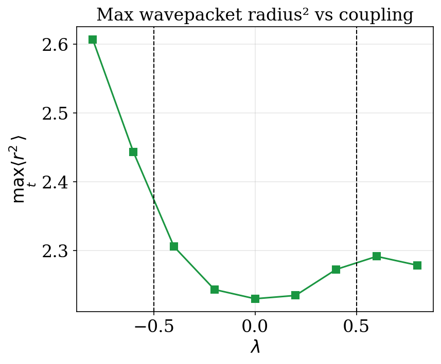
We also propagate the time-dependent Schrödinger equation directly, via the Crank–Nicolson scheme [7], which preserves discrete unitarity so that any residual norm drift is double-precision rounding rather than a physical instability. The Gaussian wavepacket of Fig. 2 exhibits $\langle\hat{x}^{2}+\hat{y}^{2}\rangle(t)$ bounded in $[1.02,2.61]$ with no secular growth, and the coupling scan of Fig. 3 extends this confinement across $\lambda\in[-0.8,+0.8]$ including well past the classical Lyapunov boundary $|\lambda|=1/2$.

VI Energy spectrum

At $\lambda=0$ the Hamiltonian separates and the spectrum is $E^{(0)}_{n_{x}n_{y}}=\hbar\omega(n_{x}-n_{y})$, unbounded in both directions with no ground state — a structural feature of the ghost sector that the interaction does not cure. For $\lambda\neq 0$ we diagonalize $\hat{H}$ in the truncated Fock basis $\{|n_{x}\rangle\otimes|n_{y}\rangle:n_{x},n_{y}\leq N_{\rm max}=21\}$ (484 states). The integrable structure implied by $\hat{C}$ predicts Poisson inter-multiplet level spacings, and this is what we find: the integer-spaced ladder of degenerate subspaces survives the interaction intact, consistent with the Poisson statistics expected for an integrable system (Fig. 4).

Figure 4: Energy spectrum of the ghost-coupled oscillator for $\lambda=1/3$, Fock basis with $N_{\rm max}=21$ (484 states). Top left: all 484 eigenvalues in the complex plane; all lie on the real axis within LAPACK precision. Top center: sorted real eigenvalues for $\lambda=0$ (grey) and $\lambda=1/3$ (red); shifts are $\lesssim 10^{-4}$, consistent with $V_{I}$ acting perturbatively. Top right: unfolded level-spacing distribution of the intra-multiplet splittings introduced by $V_{I}$, compared with Poisson $P(s)=e^{-s}$ (dashed) and Wigner-Dyson $P(s)\propto se^{-\pi s^{2}/4}$ (solid red). Within each degenerate multiplet the distribution is consistent with Wigner-Dyson, as expected from degenerate perturbation theory; the global inter-multiplet structure remains Poisson, consistent with an integrable system. Bottom row: probability density $|\phi_{n}(x,y)|^{2}$ for three low-lying eigenstates identified by maximum overlap with $|0,0\rangle$, $|1,0\rangle$, and $|0,1\rangle$, showing the expected nodal structure of harmonic oscillator product states.

All eigenvalues lie on the real axis within LAPACK precision, consistent with the PT-symmetry analysis of the continuum operator [3]; $V_{I}$ produces shifts $\lesssim 10^{-4}$ and opens no gap. (The minimum observed gap $\sim 10^{-11}$ is numerical round-off in near-degenerate diagonalization, five orders of magnitude below the perturbative splitting scale.) Low-lying eigenstates are spatially localized within the central region of the grid, providing a spectral counterpart to the dynamical wavepacket confinement of Eq. (7). The bounded phase-space moments established above therefore genuinely coexist with an unbounded, ground-state-free spectrum.

VII Discussion and conclusions

The central result of this Letter is analytic and exact: the operator $\hat{C}$ defined in Eq. (4) satisfies $[\hat{C},\hat{H}]=0$ with no $\hbar$ corrections, as a direct consequence of canonical commutation relations and the Leibniz rule alone. From this single fact, elementary operator algebra yields the bound (7): the mean squared phase-space radius $\langle\hat{x}^{2}+\hat{y}^{2}+\hat{p}_{x}^{2}+\hat{p}_{y}^{2}\rangle$ is bounded for all time, for every quantum state with finite initial second moments, at all coupling strengths, provided the time evolution is unitary.

We now state precisely what the bound does and does not establish.

What is proven. The bound (7) is a rigorous statement about second moments of the quantum state. It holds for every pure or mixed state, coherent or Fock, and reduces to the classical bound of Ref. [13] in the limit $\hbar\to 0$, since no $\hbar$-dependent terms appear in Eq. (7). There are no operator-ordering ambiguities in the proof and no perturbative remainder: the commutator $[\hat{C},\hat{H}]=0$ is exact for all $\hbar>0$.

What is not proven. The bound does not imply spectral stability, the existence of a ground state, or spatial localization of the wavefunction beyond the control of second moments: in principle the wavefunction can develop tails outside any compact region while $\langle\hat{x}^{2}+\hat{y}^{2}\rangle$ remains bounded. The question of whether $\hat{H}$ admits a self-adjoint extension on $L^{2}(\mathbb{R}^{2})$ is resolved affirmatively in Theorem 1, which establishes that unitary evolution holds in the continuum and that the bound (7) applies literally. What remains open is the construction of the positive-definite $\mathcal{CPT}$ inner product from the eigenstates of $\hat{H}$, and the extension of these results to ghost-coupled field theories including Lee-Wick models [18, 19] and the Pais-Uhlenbeck oscillator [23]. Concurrent work [12, 11] resolves two of the questions left open here, establishing a unique vacuum and a discrete (non-dense) spectrum for ghost systems with polynomial confining interactions. Whether spectral discreteness accompanies bounded second moments for the bounded, vanishing interaction $V_{I}$ of Eq. (2) is the sharpest open question left by the present work: the operator $\hat{C}$ predicts Poisson inter-multiplet statistics (confirmed numerically in Fig. 4), but a proof that the spectrum is not dense for non-confining interactions remains out of reach with current methods.

Relation to the Ostrogradsky theorem. The most natural objection to the preceding is that the Ostrogradsky theorem guarantees the Hamiltonian is unbounded below, and our spectrum confirms this. The theorem does not, however, preclude bounded phase-space moments, and our result shows explicitly that the two can coexist. Ostrogradsky instability and bounded second moments are statements about different properties of the dynamics, and the interaction structure of $V_{I}$ is precisely what allows them to be simultaneously satisfied.

Structural relevance to Lee-Wick and Pais-Uhlenbeck. The boundedness of $V_{I}$ and the existence of $\hat{C}$ both depend on the specific hyperbolic-boost-covariant combination $(x^{2}-y^{2}-1)^{2}+4x^{2}$, not on the wrong-sign kinetic term alone. Lee-Wick models [18, 19] and the Pais-Uhlenbeck oscillator [23] acquire their ghost sector from higher-derivative kinetic terms that, after reduction to a two-oscillator form, do not generically share this symmetry structure; whether physically motivated interactions in those theories can be arranged to preserve an analogous conserved operator is an open question that the present construction makes sharp. A natural intermediate step toward the field-theoretic extension is the classical field theory program of Refs. [10, 17], which establishes small-data global stability for ghostly field configurations in $(N+1)$ dimensions: the dynamical decoupling mechanism responsible for classical stability in the mechanical model persists in the field-theoretic setting, lending support to the conjecture that an analogous quantum operator bound may survive the passage to infinitely many degrees of freedom. The key obstacles specific to field theory, namely renormalization, the absence of a conserved $\hat{C}$ in the continuum limit, and the divergence of the naive vacuum decay rate, remain open and represent the sharpest targets for future work.

Relation to prior benign-ghost and pseudo-Hermiticity approaches. Two bodies of work have previously argued that ghost-coupled systems can be well-behaved. Smilga and collaborators [24, 8] identified classes of “benign ghost” mechanical systems whose classical motion remains bounded and whose quantum evolution is unitary, typically by exhibiting specific interaction forms or by restricting to islands of stability in phase space. Mostafazadeh and others in the pseudo-Hermitian / $\mathcal{PT}$-symmetric quantum mechanics program [20] obtain a stable, unitary Pais-Uhlenbeck quantization by redefining the Hilbert-space inner product, replacing the standard $L^{2}$ metric with a positive-definite $\mathcal{CPT}$-like inner product with respect to which the Hamiltonian is Hermitian. Our result is logically distinct from both approaches. The Hamiltonian studied here is self-adjoint on the standard $L^{2}(\mathbb{R}^{2})$ inner product (Theorem 1), so unitarity is inherited from the bounded-perturbation theorem rather than from a redefinition of the inner product; the bound (7) then follows from an exact operator identity $[\hat{C},\hat{H}]=0$ rather than from exact solvability or confinement to a stability island. To our knowledge, this is the first rigorous, state-independent, non-perturbative upper bound on the mean squared phase-space radius for a ghost-coupled quantum system that is not exactly solvable, obtained without modifying the inner product.

Role of the numerics. With continuum unitarity established analytically (Theorem 1), the numerical results play a complementary rather than a logically necessary role: the Heisenberg, Schrödinger, and Fock-space calculations collectively confirm that the analytic bound (7) and the integrable structure implied by $\hat{C}$ are reflected in the actual dynamics — at the Ehrenfest, wavepacket, and spectral levels, respectively.

Together these results sharpen the message of Refs. [13, 9]: ghost instability is not an inescapable consequence of a wrong-sign kinetic term, but depends critically on the interaction structure. The present work provides the first rigorous quantum-mechanical demonstration of this fact, extending the classical Lyapunov result to an exact operator bound with no $\hbar$ corrections and no perturbative remainder.

Open questions for future work include: whether $\mathcal{CPT}$ norm conservation holds pointwise in the continuum theory; a grid-refinement study of the Schrödinger propagation to verify convergence of $\langle R^{2}\rangle(t)$ as $\Delta x\to 0$; whether spectral discreteness can be established for bounded, vanishing interactions of the form studied here; and the extension of these results to ghost-coupled field theory, including Lee-Wick models and the Pais-Uhlenbeck oscillator [23]. The companion program of Refs. [12, 11] shows that confining polynomial interactions yield discrete spectra, raising the question of whether the dynamical decoupling mechanism responsible for our moment bound is also sufficient to discretize the spectrum without confining walls.

Note added. While finalizing this work we became aware of two companion papers by Deffayet, Fathe Jalali, Held, Mukohyama, and Vikman submitted concurrently [12, 11]. Reference [12] canonically quantizes a globally stable ghost oscillator with a polynomial confining interaction, proves unitarity, constructs a unique positive ground state, and establishes bounded second moments via a positive-definite integral of motion $\hat{H}_{\uparrow}$. Reference [11] proves via separability theory and WKB analysis that the energy spectrum need not be continuous or dense, constructing examples with exactly one finite accumulation point or none. The interaction studied in those works is polynomial and confining; ours is bounded and vanishes at large separations. Our bound is state-independent and requires no spectral input; the two approaches are therefore complementary rather than duplicative. Reference [12] notes our work in its closing remark.

VIII Supplemental Material:
Ghost Degrees of Freedom Without Quantum Runaway — Explicit Operator-Ordered Verification of $[\hat{C},\hat{H}]=0$

This Supplemental Material carries out the explicit operator-ordered verification that $[\hat{C},\hat{H}]=0$ with no $\hbar$ remainder, where

$$\hat{H} =\tfrac{1}{2}(\hat{p}_{x}^{2}+\hat{x}^{2})-\tfrac{1}{2}(\hat{p}_{y}^{2}+\hat{y}^{2})+V_{I}(\hat{x},\hat{y}),$$ (17)

$$\hat{C} =\hat{K}^{2}+(\hat{p}_{x}^{2}+\hat{x}^{2})-(\hat{x}^{2}-\hat{y}^{2}-1)V_{I}(\hat{x},\hat{y}),$$ (18)

$$\qquad\hat{K}=\hat{x}\hat{p}_{y}+\hat{y}\hat{p}_{x},$$ (19)

$$V_{I}(x,y)=\lambda\bigl[(x^{2}-y^{2}-1)^{2}+4x^{2}\bigr]^{-1/2}.$$ (20)

Throughout we set $\hbar=1$ and use $[\hat{x},\hat{p}_{x}]=[\hat{y},\hat{p}_{y}]=i$, with all cross-sector commutators vanishing. In Secs. I–V we carry out the operator algebra to reduce $[\hat{C},\hat{H}]$ to a sum of terms of definite momentum degree. In Sec. VI we show that each such term vanishes identically by direct substitution of Eq. (20) and the algebraic identity

$$(x^{2}-y^{2}-1)^{2}+4x^{2}-(y^{2}-x^{2})^{2}=2(x^{2}+y^{2})+1,$$ (21)

equivalently

$$\Delta\equiv(x^{2}-y^{2}-1)^{2}+4x^{2}=(x^{2}-y^{2})^{2}+2(x^{2}+y^{2})+1.$$ (22)

Notation.

We abbreviate

$$s=x^{2}+y^{2},\qquad d=x^{2}-y^{2},\qquad\Delta=d^{2}+2s+1,$$ (23)

so $V_{I}=\lambda/\sqrt{\Delta}$. We also use

$$\hat{B}=\hat{p}_{x}^{2}+\hat{x}^{2},\quad\hat{D}=\hat{p}_{y}^{2}+\hat{y}^{2},\quad\hat{M}=(\hat{x}^{2}-\hat{y}^{2}-1)V_{I}(\hat{x},\hat{y}),$$ (24)

so that $\hat{H}=\tfrac{1}{2}(\hat{B}-\hat{D})+V_{I}$ and $\hat{C}=\hat{K}^{2}+\hat{B}-\hat{M}$.

I. Preliminary commutator identities

For any smooth $f(\hat{x},\hat{y})$:

$$[\hat{\hat{p}_{x}},\hat{f}] =-i\,\partial_{x}f, [\hat{\hat{p}_{y}},\hat{f}] =-i\,\partial_{y}f,$$ (25)

$$[\hat{\hat{p}_{x}^{2}},\hat{f}] =-2i(\partial_{x}f)\,\hat{p}_{x}-\partial_{x}^{2}f, [\hat{\hat{p}_{y}^{2}},\hat{f}] =-2i(\partial_{y}f)\,\hat{p}_{y}-\partial_{y}^{2}f.$$ (26)

Equation (26) follows from (25) and $\hat{p}_{x}(\partial_{x}f)=(\partial_{x}f)\hat{p}_{x}-i\partial_{x}^{2}f$. Our convention throughout is to place position-operator functions to the left of the remaining momenta.

We also record

$$[\hat{x}^{2},f] =[\hat{y}^{2},f]=0,$$

$$[\hat{p}_{x},\hat{p}_{y}] =0,$$

$$[\hat{x},\hat{p}_{y}] =[\hat{y},\hat{p}_{x}]=0.$$ (27)

II. Decomposition of $[\hat{C},\hat{H}]$

Using the decomposition above,

$$[\hat{C},\hat{H}] =\tfrac{1}{2}[\hat{K}^{2},\hat{B}-\hat{D}]+[\hat{K}^{2},V_{I}]$$

$$\quad+\tfrac{1}{2}[\hat{B},\hat{B}-\hat{D}]+[\hat{B},V_{I}]$$

$$\quad-\tfrac{1}{2}[\hat{M},\hat{B}-\hat{D}]-[\hat{M},V_{I}].$$ (28)

Two terms vanish immediately: $[\hat{B},\hat{B}-\hat{D}]=0$ (because $[\hat{B},\hat{D}]=0$ since the $x$- and $y$-sectors commute), and $[\hat{\hat{M}},\hat{V_{I}}]=0$ (both are functions of commuting position operators). We show next that $[\hat{K}^{2},{\hat{B}-\hat{D}}]$ also vanishes identically. This leaves only three nontrivial contributions, which we evaluate in Secs. IV–V.

III. The identity $[\hat{K}^{2},\hat{B}-\hat{D}]=0$

A direct calculation gives

$$[\hat{K},\hat{B}] =[\hat{x}\hat{p}_{y}+\hat{y}\hat{p}_{x},\,\hat{p}_{x}^{2}+\hat{x}^{2}]$$

$$=[\hat{x},\hat{p}_{x}^{2}]\hat{p}_{y}+\hat{y}[\hat{p}_{x},\hat{x}^{2}]$$

$$=2i\hat{p}_{x}\hat{p}_{y}-2i\hat{x}\hat{y}=2i(\hat{p}_{x}\hat{p}_{y}-\hat{x}\hat{y}),$$ (29)

where we used $[\hat{\hat{x}},\hat{\hat{p}_{x}^{2}}]=2i\hat{p}_{x}$, $[\hat{\hat{p}_{x}},\hat{\hat{x}^{2}}]=-2i\hat{x}$, and the fact that cross-sector operators commute. An entirely analogous computation gives

$$[\hat{\hat{K}},\hat{\hat{D}}]=-2i\hat{x}\hat{y}+2i\hat{p}_{x}\hat{p}_{y}=2i(\hat{p}_{x}\hat{p}_{y}-\hat{x}\hat{y}).$$ (30)

Therefore

$$[\hat{K},\hat{B}-\hat{D}]=0,$$ (31)

and consequently

$$[\hat{K}^{2},\hat{B}-\hat{D}] =\hat{K}[\hat{K},\hat{B}-\hat{D}]+[\hat{K},\hat{B}-\hat{D}]\hat{K}$$

$$=0.$$ (32)

The decomposition (28) reduces to

$$\boxed{\ [\hat{C},\hat{H}]=[\hat{K}^{2},V_{I}]+[\hat{B},V_{I}]-\tfrac{1}{2}[\hat{M},\hat{B}-\hat{D}].\ }$$ (33)

IV. Evaluation of $[\hat{B},V_{I}]$ and $[\hat{M},\hat{B}-\hat{D}]$

Since $V_{I}$ and $\hat{M}$ are multiplication operators, from (26) together with $[\hat{\hat{x}^{2}},\hat{V_{I}}]=0$:

$$[\hat{B},V_{I}] =[\hat{p}_{x}^{2},V_{I}]=-2i(\partial_{x}V_{I})\hat{p}_{x}-\partial_{x}^{2}V_{I}.$$ (34)

Similarly,

$$[\hat{M},\hat{B}-\hat{D}] =2i(\partial_{x}M)\hat{p}_{x}+\partial_{x}^{2}M$$

$$\quad-2i(\partial_{y}M)\hat{p}_{y}-\partial_{y}^{2}M.$$ (35)

With $M=(x^{2}-y^{2}-1)V_{I}$,

$$\partial_{x}M =2xV_{I}+(x^{2}-y^{2}-1)\partial_{x}V_{I},$$ (36)

$$\partial_{y}M =-2yV_{I}+(x^{2}-y^{2}-1)\partial_{y}V_{I},$$ (37)

$$\partial_{x}^{2}M =2V_{I}+4x\,\partial_{x}V_{I}+(x^{2}-y^{2}-1)\partial_{x}^{2}V_{I},$$ (38)

$$\partial_{y}^{2}M =-2V_{I}-4y\,\partial_{y}V_{I}+(x^{2}-y^{2}-1)\partial_{y}^{2}V_{I}.$$ (39)

V. Evaluation of $[\hat{K}^{2},V_{I}]$

Using $[\hat{\hat{K}},\hat{V_{I}}]=\hat{x}[\hat{\hat{p}_{y}},\hat{V_{I}}]+\hat{y}[\hat{\hat{p}_{x}},\hat{V_{I}}]=-iu$, where

$$u(x,y)\equiv x\,\partial_{y}V_{I}+y\,\partial_{x}V_{I},$$ (40)

we obtain $[\hat{\hat{K}^{2}},\hat{V_{I}}]=\hat{K}[\hat{\hat{K}},\hat{V_{I}}]+[\hat{\hat{K}},\hat{V_{I}}]\hat{K}=-i(\hat{K}u+u\hat{K})$. Expanding the anticommutator with position-ordered ordering:

$$\hat{K}u+u\hat{K} =\hat{x}(\hat{p}_{y}u+u\hat{p}_{y})+\hat{y}(\hat{p}_{x}u+u\hat{p}_{x})$$

$$=2\hat{x}u\hat{p}_{y}+2\hat{y}u\hat{p}_{x}-i(\hat{x}\partial_{y}u+\hat{y}\partial_{x}u),$$ (41)

where we used $\hat{p}_{y}u=u\hat{p}_{y}-i\partial_{y}u$ etc. Hence

$$[\hat{\hat{K}^{2}},\hat{V_{I}}]=-2i(\hat{x}u\hat{p}_{y}+\hat{y}u\hat{p}_{x})-(\hat{x}\partial_{y}u+\hat{y}\partial_{x}u).$$ (42)

Substituting the definition of $u$:

$$\hat{x}u =\hat{x}^{2}\partial_{y}V_{I}+\hat{x}\hat{y}\partial_{x}V_{I},$$ (43)

$$\hat{y}u =\hat{x}\hat{y}\partial_{y}V_{I}+\hat{y}^{2}\partial_{x}V_{I},$$ (44)

$$\hat{x}\partial_{y}u+\hat{y}\partial_{x}u =\hat{x}^{2}\partial_{y}^{2}V_{I}+\hat{y}^{2}\partial_{x}^{2}V_{I}$$

$$\quad+2\hat{x}\hat{y}\,\partial_{x}\partial_{y}V_{I}+\hat{x}\partial_{x}V_{I}+\hat{y}\partial_{y}V_{I},$$ (45)

so that

$$[\hat{K}^{2},V_{I}] =-2i\bigl[\hat{x}^{2}(\partial_{y}V_{I})\hat{p}_{y}+\hat{x}\hat{y}(\partial_{x}V_{I})\hat{p}_{y}$$

$$\qquad\quad+\hat{x}\hat{y}(\partial_{y}V_{I})\hat{p}_{x}+\hat{y}^{2}(\partial_{x}V_{I})\hat{p}_{x}\bigr]$$

$$\quad-\bigl[\hat{x}^{2}\partial_{y}^{2}V_{I}+\hat{y}^{2}\partial_{x}^{2}V_{I}$$

$$\qquad\quad+2\hat{x}\hat{y}\,\partial_{x}\partial_{y}V_{I}+\hat{x}\partial_{x}V_{I}+\hat{y}\partial_{y}V_{I}\bigr].$$ (46)

VI. Explicit cancellation, order by order in momenta

Summing Eqs. (34), (35), and (46) according to Eq. (33) yields

$$[\hat{\hat{C}},\hat{\hat{H}}]=\mathcal{A}_{x}\,\hat{p}_{x}+\mathcal{A}_{y}\,\hat{p}_{y}+\mathcal{A}_{0},$$ (47)

where the coefficient functions are

$$\mathcal{A}_{x} =-i\bigl[(1+x^{2}+y^{2})\partial_{x}V_{I}+2xy\,\partial_{y}V_{I}+2xV_{I}\bigr],$$ (48)

$$\mathcal{A}_{y} =-i\bigl[(1+x^{2}+y^{2})\partial_{y}V_{I}+2xy\,\partial_{x}V_{I}+2yV_{I}\bigr],$$ (49)

$$\mathcal{A}_{0} =-2V_{I}-3x\,\partial_{x}V_{I}-3y\,\partial_{y}V_{I}$$

$$\quad\quad-\tfrac{1+x^{2}+y^{2}}{2}(\partial_{x}^{2}V_{I}+\partial_{y}^{2}V_{I})$$

$$\hskip 60.00009pt-2xy\,\partial_{x}\partial_{y}V_{I}.$$ (50)

The coefficients of $\hat{p}_{x}$, $\hat{p}_{y}$, and the identity are independent operator structures, so $[\hat{C},\hat{H}]=0$ is equivalent to the three scalar identities $\mathcal{A}_{x}\equiv 0$, $\mathcal{A}_{y}\equiv 0$, and $\mathcal{A}_{0}\equiv 0$. We verify each in turn.

A. Derivatives of $V_{I}$

From $V_{I}=\lambda\Delta^{-1/2}$ and $\Delta=d^{2}+2s+1$ with $d=x^{2}-y^{2}$, $s=x^{2}+y^{2}$,

$$\partial_{x}\Delta=4x(d+1),\qquad\partial_{y}\Delta=4y(1-d),$$ (51)

giving

$$\partial_{x}V_{I}=-\frac{2\lambda x(d+1)}{\Delta^{3/2}},\qquad\partial_{y}V_{I}=-\frac{2\lambda y(1-d)}{\Delta^{3/2}}.$$ (52)

B. Vanishing of $\mathcal{A}_{x}$

Multiplying Eq. (48) through by $\Delta^{3/2}/\lambda$ and using (52):

$$\frac{\Delta^{3/2}}{\lambda}\,\frac{\mathcal{A}_{x}}{-i} =-2x(1+s)(d+1)-4xy^{2}(1-d)+2x\Delta$$

$$=2x\bigl[\Delta-(1+s)(d+1)-2y^{2}(1-d)\bigr].$$ (53)

Expanding the bracket using $(1+s)(d+1)=d+1+sd+s$, $2y^{2}(1-d)=2y^{2}-2y^{2}d$, and $\Delta=d^{2}+2s+1$:

$$\Delta-(1+s)(d+1)-2y^{2}(1-d)$$

$$\quad=d^{2}+s-d-sd-2y^{2}+2y^{2}d.$$ (54)

Substituting $2y^{2}=s-d$:

$$\quad=d^{2}+s-d-sd-(s-d)+(s-d)d$$

$$\quad=d^{2}+s-d-sd-s+d+sd-d^{2}=0.$$ (55)

Hence $\mathcal{A}_{x}\equiv 0$.

C. Vanishing of $\mathcal{A}_{y}$

Multiplying Eq. (49) through by $\Delta^{3/2}/\lambda$:

$$\frac{\Delta^{3/2}}{\lambda}\,\frac{\mathcal{A}_{y}}{-i} =-2y(1+s)(1-d)-4x^{2}y(d+1)+2y\Delta$$

$$=2y\bigl[\Delta-(1+s)(1-d)-2x^{2}(d+1)\bigr].$$ (56)

Expanding with $(1+s)(1-d)=1-d+s-sd$ and $2x^{2}(d+1)=2x^{2}d+2x^{2}$, substituting $2x^{2}=s+d$:

$$\Delta-(1+s)(1-d)-2x^{2}(d+1)$$

$$\quad=d^{2}+s+d+sd-sd-d^{2}-s-d=0.$$ (57)

Hence $\mathcal{A}_{y}\equiv 0$.

D. Vanishing of $\mathcal{A}_{0}$: second derivatives

We need the second derivatives of $V_{I}$. Differentiating (52) and using $\partial_{x}^{2}\Delta=12x^{2}-4y^{2}+4$, $\partial_{y}^{2}\Delta=12y^{2}-4x^{2}+4$, $\partial_{x}\partial_{y}\Delta=-8xy$:

$$\partial_{x}^{2}\Delta+\partial_{y}^{2}\Delta =8(s+1),$$ (58)

$$(\partial_{x}\Delta)^{2}+(\partial_{y}\Delta)^{2} =16\bigl[x^{2}(d+1)^{2}+y^{2}(1-d)^{2}\bigr]$$

$$=16\bigl[d^{2}(s+2)+s\bigr]$$

$$=16\bigl[\Delta(s+2)-2(s+1)^{2}\bigr],$$ (59)

where the last step uses $d^{2}=\Delta-2s-1$. Then

$$\partial_{x}^{2}V_{I}+\partial_{y}^{2}V_{I} =-\frac{\lambda(\partial_{x}^{2}\Delta+\partial_{y}^{2}\Delta)}{2\Delta^{3/2}}+\frac{3\lambda\bigl[(\partial_{x}\Delta)^{2}+(\partial_{y}\Delta)^{2}\bigr]}{4\Delta^{5/2}}$$

$$=\frac{4\lambda(2s+5)}{\Delta^{3/2}}-\frac{24\lambda(s+1)^{2}}{\Delta^{5/2}}.$$ (60)

For the cross term, $\partial_{x}\Delta\cdot\partial_{y}\Delta=16xy(1-d^{2})=16xy\bigl[2(s+1)-\Delta\bigr]$, and $\partial_{x}\partial_{y}\Delta=-8xy$, giving

$$\partial_{x}\partial_{y}V_{I}=-\frac{\lambda\partial_{x}\partial_{y}\Delta}{2\Delta^{3/2}}+\frac{3\lambda\,\partial_{x}\Delta\,\partial_{y}\Delta}{4\Delta^{5/2}}=-\frac{8\lambda xy}{\Delta^{3/2}}+\frac{24\lambda xy(s+1)}{\Delta^{5/2}}.$$ (61)

E. Vanishing of $\mathcal{A}_{0}$: assembly

Substituting (52), (60), and (61) into (50), and factoring $\lambda$:

$$\mathcal{A}_{0}/\lambda =-\frac{2}{\Delta^{1/2}}+\frac{6x^{2}(d+1)}{\Delta^{3/2}}+\frac{6y^{2}(1-d)}{\Delta^{3/2}}$$

$$\quad-\frac{2(s+1)(2s+5)}{\Delta^{3/2}}+\frac{12(s+1)^{3}}{\Delta^{5/2}}$$

$$\quad+\frac{16x^{2}y^{2}}{\Delta^{3/2}}-\frac{48x^{2}y^{2}(s+1)}{\Delta^{5/2}}$$

$$=\frac{-2\Delta+6(d^{2}+s)-2(s+1)(2s+5)+16x^{2}y^{2}}{\Delta^{3/2}}$$

$$\quad+\frac{12(s+1)^{3}-48x^{2}y^{2}(s+1)}{\Delta^{5/2}}.$$ (62)

Now observe that $x^{2}(d+1)+y^{2}(1-d)=d^{2}+s$, so the $\Delta^{-3/2}$ numerator in Eq. (62) is

$$-2\Delta+6(d^{2}+s)-2(s+1)(2s+5)+16x^{2}y^{2}$$

$$\qquad=-2d^{2}-4s-2+6d^{2}+6s-4s^{2}-14s-10+16x^{2}y^{2}$$

$$\qquad=4d^{2}-12s-12-4s^{2}+16x^{2}y^{2}.$$ (63)

Using $d^{2}=s^{2}-4x^{2}y^{2}$ (which is equivalent to $(x^{2}-y^{2})^{2}=(x^{2}+y^{2})^{2}-4x^{2}y^{2}$), $4d^{2}=4s^{2}-16x^{2}y^{2}$, so

$$4d^{2}-4s^{2}+16x^{2}y^{2}=0,$$ (64)

and the numerator of the $\Delta^{-3/2}$ piece collapses to $-12s-12=-12(s+1)$.

Therefore

$$\mathcal{A}_{0}/\lambda=-\frac{12(s+1)}{\Delta^{3/2}}+\frac{12(s+1)\bigl[(s+1)^{2}-4x^{2}y^{2}\bigr]}{\Delta^{5/2}}.$$ (65)

The key algebraic fact is

$$(s+1)^{2}-4x^{2}y^{2}=s^{2}+2s+1-4x^{2}y^{2}=d^{2}+2s+1=\Delta,$$ (66)

using again $s^{2}-4x^{2}y^{2}=d^{2}$. Hence the $\Delta^{-5/2}$ term equals $12(s+1)\Delta/\Delta^{5/2}=12(s+1)/\Delta^{3/2}$, and

$$\mathcal{A}_{0}/\lambda=-\frac{12(s+1)}{\Delta^{3/2}}+\frac{12(s+1)}{\Delta^{3/2}}=0.$$ (67)

F. Conclusion

Combining Secs. VI.B–E, all three coefficient functions in Eq. (47) vanish identically:

$$\mathcal{A}_{x}\equiv 0,\qquad\mathcal{A}_{y}\equiv 0,\qquad\mathcal{A}_{0}\equiv 0,$$ (68)

and therefore, as an operator identity on the common invariant core $\mathcal{D}_{\rm fin}=\mathrm{span}\{h_{n}(\hat{x})h_{m}(\hat{y}):n,m\geq 0\}$,

$$\boxed{\ [\hat{C},\hat{H}]=0.\ }$$ (69)

Because $\hat{C}$ is at most quadratic in momenta, the operator computation above truncates: no higher than first derivatives of $V_{I}$ enter the momentum-linear pieces $\mathcal{A}_{x}\hat{p}_{x}+\mathcal{A}_{y}\hat{p}_{y}$, and no higher than second derivatives enter the $\mathcal{A}_{0}$ piece, with all three pieces vanishing exactly. There is no $\hbar$-dependent remainder: Eq. (69) holds as an exact operator identity, not as a leading semiclassical approximation.

Standard approximation arguments, using the self-adjointness of $\hat{H}$ on $\mathcal{D}(H_{0})$ established in Theorem 1 of the main text, extend Eq. (69) to all of $\mathcal{D}(H_{0})$. Hence, under the unitary evolution $U(t)=e^{-it\hat{H}}$ generated by Stone’s theorem, $\langle\psi_{t},\hat{C}\psi_{t}\rangle=\langle\psi_{0},\hat{C}\psi_{0}\rangle$ for every $\psi_{0}\in\mathcal{D}(\Sigma^{1/2})$.

VII. Classical cross-check: $\{C,H\}_{\rm PB}=0$

For completeness, the classical Poisson bracket $\{C,H\}_{\rm PB}$ vanishes as a consistency check of the operator identity above. The following SymPy script verifies this symbolically:

⬇

from sympy import symbols, diff, simplify, Rational

x, y, px, py, lam = symbols(’x’y’px’py’lam’, real=True)

V = lam/((x**2-y**2-1)**2 + 4*x**2)**Rational(1,2)

H = (px**2+x**2)/2 - (py**2+y**2)/2 + V

K = py*x + px*y

C = K**2 + (px**2+x**2) - (x**2-y**2-1)*V

def PB(A, B):

return (diff(A,x)*diff(B,px) - diff(A,px)*diff(B,x)

+ diff(A,y)*diff(B,py) - diff(A,py)*diff(B,y))

print(simplify(PB(C, H))) # prints 0

This agrees with the $\hbar^{0}$ limit of the operator identity: the coefficients of $\hat{p}_{x}$ and $\hat{p}_{y}$ in $\mathcal{A}_{x},\mathcal{A}_{y}$ are precisely (up to factors of $-i$) the position-space content of $\{C,H\}_{\rm PB}$, while $\mathcal{A}_{0}$ represents the quantum correction that would naively be of order $\hbar^{2}$ but here also vanishes because of the geometric identity (21).