A Lightning-Fast Three-Flavor Neutrino Oscillation Calculator in Constant-Density Matter with Built-In Uncertainty Propagation

Abstract

Neutrino oscillation experiments are entering an era of precision, requiring both fast calculations and reliable uncertainty estimates. We present a compact three-flavor oscillation calculator for constant-density matter, built on analytic perturbative formulas and validated against established series expansions. Using the NuFIT 6.0 global-fit covariance matrix, the tool incorporates up-to-date parameter values and correlations.

It accurately computes appearance and disappearance probabilities over 0.3–5 GeV at a 295 km baseline, offering two computation modes: exact Hamiltonian diagonalization for high-fidelity results, and a faster perturbative approximation that runs roughly 27$\times$ quicker. A hybrid scheme handles the MSW resonance region, combining speed with accuracy.

Uncertainties can be propagated via Monte Carlo sampling or a fast linearized approach, producing reliable confidence bands. The implementation preserves unitarity, reproduces vacuum and resonance limits, and captures high-energy suppression effects.

This calculator provides a fast, reliable framework for parameter scans, phenomenological studies, and sensitivity estimates for current and future long-baseline experiments like Hyper-Kamiokande and DUNE.

1 Introduction

The discovery of neutrino oscillations stands as one of the most consequential achievements of twentieth-century particle physics, establishing beyond doubt that neutrinos possess non-zero masses and that lepton flavor is not conserved during free propagation. These observations constitute direct evidence for physics beyond the Standard Model, whose original formulation predicted massless neutrinos with exactly conserved individual lepton numbers. The theoretical framework for neutrino flavor conversion was pioneered by Pontecorvo Pontecorvo1958 , who proposed in the late 1950s that neutrinos could undergo quantum-mechanical oscillations between flavor states, in direct analogy to the $K^{0}$–$\bar{K}^{0}$ mixing system. This idea was extended to the three-generation mixing framework by Maki, Nakagawa, and Sakata, giving rise to the PMNS mixing matrix that now bears their joint names.

Experimental confirmation of the oscillation mechanism arrived through two landmark measurements in the late 1990s and early 2000s. The Super-Kamiokande collaboration SuperK1998 reported a highly significant up–down asymmetry in the flux of atmospheric muon neutrinos, consistent with near-maximal $\nu_{\mu}\to\nu_{\tau}$ oscillations over baseline distances of order $10^{4}$ km. Simultaneously, the Sudbury Neutrino Observatory SNO2002 measured the total active neutrino flux from the sun using neutral-current interactions and demonstrated that the deficit previously observed in the charged-current solar neutrino rate was entirely attributable to flavor transformation rather than a reduction in the solar flux. Together, these results established the three-flavor mixing framework and launched a worldwide experimental program to precisely measure the parameters of the lepton mixing matrix.

The subsequent two decades of precision measurements have dramatically refined our knowledge of the oscillation parameters. The T2K experiment T2K2011 at the 295 km Tokai-to-Kamioka baseline and the NOvA experiment NOvA2005 at 810 km have measured the atmospheric mixing parameters $\theta_{23}$ and $\Delta m^{2}_{31}$ and provided the first sensitivity to the Dirac CP-violating phase $\delta_{CP}$. The reactor neutrino experiments Daya Bay DayaBay2012 , RENO RENO2012 , and Double Chooz DoubleChooz2012 precisely measured the reactor angle, establishing $\theta_{13}\approx 8.5^{\circ}$. This value is significant for two reasons: it is large enough to be measured with good statistical precision at reactor baselines, yet small enough—$\sin\theta_{13}\approx 0.148$—to serve as a natural expansion parameter in analytic perturbative approximations to the oscillation probabilities.

Matter effects, which modify the effective oscillation parameters as neutrinos propagate through ordinary matter, were introduced theoretically by Wolfenstein Wolfenstein1978 through a refractive-index formalism. Mikheyev and Smirnov MSW1985 subsequently demonstrated that under certain conditions this matter-induced modification can lead to resonant flavor conversion—the MSW effect—in which the effective mixing angle in matter approaches $\pi/4$ even when the vacuum mixing angle is small. For long-baseline accelerator experiments traversing the Earth’s crust, the matter effect is a significant and irreducible contribution to the oscillation probability that must be incorporated accurately. The charged-current forward scattering potential of electron neutrinos off electrons introduces an energy-dependent modification to the effective mixing parameters, with the resonance occurring at a specific energy $E_{\mathrm{res}}$ that depends on the matter density and the vacuum oscillation parameters.

The field now stands at a transformative moment with two flagship next-generation experiments under construction. Hyper-Kamiokande HyperK2018 , an 8.4 megaton water Cherenkov detector in the Tochibora mine in Japan, will measure the 295 km baseline from J-PARC with an exposure roughly twenty times that of T2K, providing unprecedented sensitivity to $\delta_{CP}$ and the mass ordering. The Deep Underground Neutrino Experiment (DUNE), which will direct an 80 GeV, 1.2 MW beam 1300 km through the Earth’s crust and upper mantle to a 40 kton liquid-argon time-projection chamber at the Homestake site in South Dakota, will complement Hyper-K with a very long baseline that enhances matter-effect sensitivity and provides access to the second oscillation maximum. Together, these experiments aim to determine the neutrino mass ordering at high significance, resolve the $\theta_{23}$ octant ambiguity, and measure $\delta_{CP}$ with sufficient precision to test whether CP violation in the lepton sector can explain the observed baryon asymmetry of the universe through leptogenesis.

The extraction of oscillation parameters from experimental data is computationally intensive. Neutrino event rates are computed as convolutions of oscillation probabilities with neutrino flux predictions, detector response functions, and neutrino–nucleus cross-section models. Statistical parameter inference employs Markov Chain Monte Carlo (MCMC) algorithms or nested-sampling methods such as MultiNest, each requiring $\mathcal{O}(10^{6})$ or more evaluations of the oscillation probability as a function of energy and the oscillation parameters. Sensitivity projections for future experiments typically involve $\mathcal{O}(10^{3})$ independent MCMC analyses. This computational pressure creates strong demand for oscillation calculators that can evaluate the full three-flavor probability matrix in microseconds while maintaining physical accuracy throughout the experimentally relevant energy range.

Existing computational tools address portions of this challenge. GLoBES provides a complete framework for long-baseline sensitivity studies but requires C integration and does not natively provide uncertainty bands. Prob3++ delivers fast numerical integration and is widely used in T2K analyses. nuSQuIDS solves the density-matrix evolution equation with high accuracy but has significant runtime overhead for simple constant-density geometries. None of these tools currently provides Python-native vectorization, built-in parameter uncertainty propagation anchored to NuFIT covariances, and sub-microsecond evaluation speed in a single dependency-free package suitable for direct integration into Python-based Bayesian pipelines. The present calculator is designed to fill this niche.

The perturbative approach to neutrino oscillation probabilities exploits the two small parameters $\alpha\equiv\Delta m^{2}_{21}/\Delta m^{2}_{31}\approx 0.030$ and $\sin\theta_{13}\approx 0.148$ to replace the numerical eigendecomposition with closed-form analytic expressions that can be evaluated without any matrix operations. These expressions, developed systematically by Akhmedov et al. Akhmedov2004 and cast in a particularly compact and physically transparent form by Minakata and Parke Minakata2015 , achieve percent-level accuracy across most of the experimentally relevant energy range. Their principal limitation is the failure of the expansion near the MSW resonance, where the dimensionless matter parameter $\hat{A}\equiv 2EV_{CC}/\Delta m^{2}_{31}$ approaches unity and the small denominators $(1-\hat{A})$ and $\hat{A}$ in the perturbative expressions diverge. The hybrid solver presented here addresses this limitation by transparently routing the resonance-band energy points to the exact numerical solver.

This paper is organized as follows. Section 2 defines the notation, physical constants, and NuFIT 6.0 inputs. Section 3 presents the three computation algorithms—exact diagonalization, compact perturbative approximation, and the hybrid solver—with complete pseudocode. Section 4 describes the two uncertainty propagation schemes. Section 5 reports validation tests and performance benchmarks. Section 6 discusses the scope and limitations of the constant-density approximation, the fidelity of Gaussian uncertainty propagation, and planned extensions. Section 7 summarizes the conclusions.

2 Notation and Physical Inputs

Throughout this work, Particle Data Group (PDG) conventions PDG2022 are adopted for the PMNS parameterization and mass-squared difference definitions. The weak-interaction flavor eigenstates $|\nu_{\alpha}\rangle$ ($\alpha=e,\mu,\tau$) are related to the Hamiltonian mass eigenstates $|\nu_{i}\rangle$ ($i=1,2,3$) through the unitary PMNS mixing matrix $U$:

$$|\nu_{\alpha}\rangle=\sum_{i=1}^{3}U_{\alpha i}|\nu_{i}\rangle.$$ (1)

The PDG parameterization of $U$ employs three Euler-like mixing angles $\theta_{12}$, $\theta_{13}$, $\theta_{23}$ and a single Dirac CP-violating phase $\delta_{CP}$. With the shorthand $c_{ij}\equiv\cos\theta_{ij}$ and $s_{ij}\equiv\sin\theta_{ij}$:

$$U=\begin{pmatrix}c_{12}c_{13}&s_{12}c_{13}&s_{13}e^{-i\delta_{CP}}\\[4.0pt] -s_{12}c_{23}-c_{12}s_{23}s_{13}e^{i\delta_{CP}}&c_{12}c_{23}-s_{12}s_{23}s_{13}e^{i\delta_{CP}}&s_{23}c_{13}\\[4.0pt] s_{12}s_{23}-c_{12}c_{23}s_{13}e^{i\delta_{CP}}&-c_{12}s_{23}-s_{12}c_{23}s_{13}e^{i\delta_{CP}}&c_{23}c_{13}\end{pmatrix}.$$ (2)

Mass-squared differences are defined as $\Delta m^{2}_{21}\equiv m^{2}_{2}-m^{2}_{1}$ and $\Delta m^{2}_{31}\equiv m^{2}_{3}-m^{2}_{1}$. The NuFIT 6.0 NuFIT2024 best-fit values for normal mass ordering are adopted as the default inputs: $\theta_{12}=33.68^{\circ}\pm 0.70^{\circ}$, $\theta_{13}=8.52^{\circ}\pm 0.11^{\circ}$, $\theta_{23}=48.5^{\circ}\pm 0.9^{\circ}$, $\delta_{CP}=177^{\circ}\,{}^{+19^{\circ}}_{-20^{\circ}}$, $\Delta m^{2}_{21}=(7.49\pm 0.19)\times 10^{-5}$ eV², and $\Delta m^{2}_{31}=(2.534\pm 0.025)\times 10^{-3}$ eV².

The reference matter configuration corresponds to the average crustal density along the Tokai–Kamioka baseline: $\rho=2.6$ g cm^-3 with electron fraction $Y_{e}=0.5$. The charged-current (CC) forward-scattering potential, which enters through coherent elastic scattering of $\nu_{e}$ off electrons, is:

$$V_{CC}=\sqrt{2}\,G_{F}\,\frac{\rho Y_{e}}{m_{N}},$$ (3)

where $G_{F}=1.1663787\times 10^{-5}$ GeV^-2 is the Fermi coupling constant and $m_{N}\approx 0.939$ GeV is the nucleon mass. The relevant NC potential difference $V_{NC}$ is flavor-universal and can be absorbed into a redefinition of the reference energy without affecting oscillation probabilities; it is therefore omitted. In natural units, the flavor-basis effective Hamiltonian at neutrino energy $E$ is:

$$H_{f}=\frac{U\,\mathrm{diag}(0,\,\Delta m^{2}_{21},\,\Delta m^{2}_{31})\,U^{\dagger}}{2E}+\mathrm{diag}(V_{CC},\,0,\,0).$$ (4)

The evolution operator over propagation distance $L$ is $S=\exp(-iH_{f}L)$, and the oscillation probability matrix is $P_{\alpha\beta}=|S_{\beta\alpha}|^{2}$. Throughout, the unit conversion $1\,\mathrm{km}=5.07\times 10^{12}\,\mathrm{eV}^{-1}$ is applied.

Two dimensionless parameters govern the physics. The hierarchy ratio $\alpha\equiv\Delta m^{2}_{21}/\Delta m^{2}_{31}\approx 0.030$ measures the ratio of the solar to the atmospheric mass-squared splitting and controls the validity of perturbative expansions in powers of $\alpha$. The dimensionless matter parameter $\hat{A}\equiv 2EV_{CC}/\Delta m^{2}_{31}$ compares the matter potential to the atmospheric oscillation frequency; the MSW resonance condition is $\hat{A}=\cos 2\theta_{13}$, corresponding to a resonance energy:

$$E_{\mathrm{res}}=\frac{\Delta m^{2}_{31}\cos 2\theta_{13}}{2V_{CC}}\approx 0.6\,\mathrm{GeV}\qquad(L=295\,\mathrm{km},\;\rho=2.6\,\mathrm{g\,cm}^{-3}).$$ (5)

At this energy, the effective matter-modified mixing angle $\theta_{13,\mathrm{eff}}\to\pi/4$ and the appearance probability is maximally enhanced.

3 Algorithms

3.1 Exact Hamiltonian Diagonalization

The exact solver constructs the full three-flavor Hamiltonian in the flavor basis, enforces Hermiticity by symmetrization to suppress floating-point anti-Hermitian noise, diagonalizes via the eigh eigensolver to obtain real eigenvalues and a unitary eigenvector matrix, and exponentiates to form the unitary time-evolution operator. Probability conservation is guaranteed at the algebraic level by the unitarity of the eigenvector matrix.

Algorithm 1 Exact Hamiltonian Diagonalization

1:Input: $E,\,L,\,\rho,\,Y_{e},\,\theta_{12},\,\theta_{13},\,\theta_{23},\,\delta_{CP},\,\Delta m^{2}_{21},\,\Delta m^{2}_{31}$

2:$V_{CC}\leftarrow\sqrt{2}\,G_{F}\,(\rho Y_{e}/m_{N})$

3:$U\leftarrow$ PMNS matrix [eq. (2), PDG convention]

4:$H_{\mathrm{vac}}\leftarrow(1/2E)\,U\,\mathrm{diag}(0,\Delta m^{2}_{21},\Delta m^{2}_{31})\,U^{\dagger}$

5:$H_{f}\leftarrow H_{\mathrm{vac}}+\mathrm{diag}(V_{CC},\,0,\,0)$

6:$H_{f}\leftarrow(H_{f}+H_{f}^{\dagger})/2$ $\triangleright$ enforce Hermiticity

7:$[\lambda_{i},\,V]\leftarrow\mathrm{eigh}(H_{f})$ $\triangleright$ real eigenvalues, unitary $V$

8:$S\leftarrow V\,\mathrm{diag}(e^{-i\lambda_{i}L})\,V^{\dagger}$

9:$P_{\alpha\beta}\leftarrow|S_{\beta\alpha}|^{2}$ for $\alpha,\beta\in\{e,\mu,\tau\}$

10:Output: $P_{\alpha\beta}$ (full $3\times 3$ probability matrix)

At the reference point $E=1$ GeV, $L=295$ km, $\rho=2.6$ g cm^-3 with NuFIT 6.0 best-fit parameters, the exact solver returns $P_{\mu e}=0.025$. Unitarity $\sum_{\beta}P_{\alpha\beta}=1$ is preserved to better than $10^{-10}$ across all tested energy and density configurations. The vectorized NumPy implementation processes an $N$-point energy array as a batched $(N\times 3\times 3)$ complex matrix operation, exploiting NumPy’s broadcasting for the exponentiation step and entirely avoiding Python-level energy loops.

The physical justification for the symmetrization step in line 5 is as follows. The flavor evolution equation $i\,d\nu/dx=H_{f}\nu$ admits a unitary solution $S(x)=\exp(-iH_{f}x)$ if and only if $H_{f}$ is exactly Hermitian. By construction, $H_{f}=H_{\mathrm{vac}}+\mathrm{diag}(V_{CC},0,0)$ is Hermitian: the vacuum term is Hermitian because $H_{\mathrm{vac}}=(1/2E)UM^{2}U^{\dagger}$ with $M^{2}=\mathrm{diag}(0,\Delta m^{2}_{21},\Delta m^{2}_{31})$ real and diagonal and $U$ unitary, and the matter term is real diagonal. However, floating-point arithmetic in the trigonometric construction of $U$ introduces anti-Hermitian rounding errors at the level of machine epsilon, $\mathcal{O}(10^{-16})$. Without correction, these accumulate through the eigendecomposition and matrix exponentiation to unitarity violations of $\mathcal{O}(10^{-8})$. The symmetrization $H_{f}\leftarrow(H_{f}+H_{f}^{\dagger})/2$ projects onto the nearest Hermitian matrix in the Frobenius norm, removing the numerical anti-Hermitian component without altering the physical content.

3.2 Compact Perturbative Approximation

The perturbative approximation replaces the numerical eigendecomposition with closed-form analytic expressions, exploiting the smallness of $\alpha\approx 0.030$ and $\sin\theta_{13}\approx 0.148$ following the formalisms of Minakata and Parke Minakata2015 and Akhmedov et al. Akhmedov2004 . Three auxiliary variables are defined to absorb the combination of physical parameters:

$$\Delta=\frac{\Delta m^{2}_{31}L}{4E},\qquad\hat{A}=\frac{2EV_{CC}}{\Delta m^{2}_{31}},\qquad J_{CP}=s_{12}c_{12}s_{23}c_{23}s_{13}c^{2}_{13}.$$ (6)

Here $\Delta$ is the atmospheric oscillation phase accumulated over baseline $L$ at energy $E$; $\hat{A}$ is the dimensionless matter parameter; and $J_{CP}$ is the Jarlskog-like invariant combination that controls the strength of CP-violating interference. The appearance probability $P_{\mu e}$ is expressed as a sum of three physically distinct contributions, expanded systematically to $\mathcal{O}(\alpha^{2})$:

$$P_{\mu e}\approx\; \underbrace{4s^{2}_{23}s^{2}_{13}\frac{\sin^{2}[(1-\hat{A})\Delta]}{(1-\hat{A})^{2}}}_{T_{\mathrm{atm}}}$$

$$+\; \underbrace{8\alpha J_{CP}\cos(\Delta+\delta_{CP})\frac{\sin(\hat{A}\Delta)}{\hat{A}}\frac{\sin[(1-\hat{A})\Delta]}{(1-\hat{A})}}_{T_{\mathrm{int}}}$$

$$+\; \underbrace{\alpha^{2}c^{2}_{23}\sin^{2}(2\theta_{12})\frac{\sin^{2}(\hat{A}\Delta)}{\hat{A}^{2}}}_{T_{\mathrm{sol}}}.$$ (7)

The term $T_{\mathrm{atm}}$ is the leading atmospheric contribution, controlled by $\theta_{13}$ and $\theta_{23}$ and matter-modified by the $(1-\hat{A})$ denominator that encodes the MSW enhancement. The term $T_{\mathrm{int}}$ is the $\mathcal{O}(\alpha)$ CP-violating interference between the atmospheric and solar oscillation channels, which carries the sensitivity to $\delta_{CP}$ and is therefore the key observable for CP-violation searches at long-baseline experiments. The term $T_{\mathrm{sol}}$ is the $\mathcal{O}(\alpha^{2})$ solar contribution, controlled by $\theta_{12}$ and sub-dominant at the 295 km baseline. For the disappearance channel, the leading-order expression:

$$P_{\mu\mu}\approx 1-4c^{2}_{13}s^{2}_{23}\left(1-c^{2}_{13}s^{2}_{23}\right)\sin^{2}(\Delta)$$ (8)

provides percent-level accuracy across the 0.3–5 GeV range.

Algorithm 2 Compact Perturbative Approximation

1:Input: same as Algorithm 1

2:$\alpha\leftarrow\Delta m^{2}_{21}/\Delta m^{2}_{31}$

3:$\Delta,\,\hat{A},\,J_{CP}\leftarrow$ eq. (6)

4:$T_{\mathrm{atm}},\,T_{\mathrm{int}},\,T_{\mathrm{sol}}\leftarrow$ eq. (7) Minakata2015 ; Akhmedov2004

5:$P_{\mu e}\leftarrow T_{\mathrm{atm}}+T_{\mathrm{int}}+T_{\mathrm{sol}}$

6:$P_{\mu\mu}\leftarrow$ eq. (8)

7:Output: $P_{\mu e},\,P_{\mu\mu}$

At $E=1$ GeV, the perturbative approximation gives $P_{\mu e}\approx 0.024$, within 5% of the exact value. Across 0.3–5 GeV, the absolute error satisfies $|\Delta P|<0.01$ everywhere outside the MSW resonance. The expansion breaks down near resonance ($\hat{A}\approx 1$), where the denominators $(1-\hat{A})$ and $\hat{A}$ in $T_{\mathrm{atm}}$ and $T_{\mathrm{int}}$ cause the perturbative expressions to diverge unphysically.

3.3 Hybrid Solver

The hybrid solver routes each energy grid point to either the perturbative or exact path based on the criterion $|\hat{A}(E)-1|<\varepsilon$, with default threshold $\varepsilon=0.15$.

Algorithm 3 Hybrid Solver

1:Input: $E,\,L,\,\rho,\,Y_{e}$, oscillation parameters, $\varepsilon=0.15$

2:Compute $V_{CC}$ via eq. (3)

3:$\hat{A}(E)\leftarrow 2E\,V_{CC}/\Delta m^{2}_{31}$ for all $E$ in grid

4:$\mathcal{M}_{\mathrm{res}}\leftarrow\{k:|\hat{A}(E_{k})-1|<\varepsilon\}$

5:for $k\in\mathcal{M}_{\mathrm{res}}$ do

6:  $P_{k}\leftarrow$ Algorithm 1 (exact)

7:end for

8:for $k\notin\mathcal{M}_{\mathrm{res}}$ do

9:  $P_{k}\leftarrow$ Algorithm 2 (perturbative)

10:end for

11:Assemble $P_{\mu e}(E),\,P_{\mu\mu}(E)$ over full grid

12:Output: probability arrays

The binary mask implementation ensures no discontinuity at the switching boundary. Figure 1 confirms that the hybrid curve follows the exact result continuously through the resonance without visible discontinuity, while tracking the perturbative curve elsewhere. The threshold $\varepsilon=0.15$ was selected empirically to ensure the hybrid error is suppressed below $10^{-3}\%$ throughout the resonance band while activating the exact solver for approximately 10% of a typical energy grid.

Figure 1: Overlay of exact diagonalization (solid black), $\mathcal{O}(\alpha^{2})$ perturbative (dashed red), and hybrid solver (dotted green) appearance probabilities $P(\nu_{\mu}\to\nu_{e})$ as a function of neutrino energy at $L=295$ km. The hybrid solver follows the exact curve through the MSW resonance without discontinuity.

4 Uncertainty Propagation

4.1 Monte Carlo Sampling

The Monte Carlo approach draws $N$ samples from the six-dimensional multivariate Gaussian defined by the NuFIT 6.0 NuFIT2024 best-fit parameter vector $\boldsymbol{\mu}$ and covariance matrix $\boldsymbol{\Sigma}_{\mathrm{params}}$, evaluates the oscillation probability for each sample, and reports the mean and percentile bands.

Algorithm 4 Monte Carlo Uncertainty Propagation

1:Input: $\boldsymbol{\mu}$ (best-fit), $\boldsymbol{\Sigma}_{\mathrm{params}}$ (NuFIT 6.0 covariance NuFIT2024 ), $N$, $E_{\mathrm{grid}}$, $L$, $\rho$

2:Initialize $P_{\mathrm{samples}}[N][|E_{\mathrm{grid}}|]$

3:for $i=1$ to $N$ do

4:  Draw $p_{i}\sim\mathcal{N}(\boldsymbol{\mu},\boldsymbol{\Sigma}_{\mathrm{params}})$ $\triangleright$ multivariate Gaussian

5:  Wrap $\delta_{CP}\in[0,2\pi)$; clip mixing angles $\in[0,\pi/2]$

6:  Compute $P_{i}(E_{k})$ via Algorithm 2 for each $E_{k}$

7:end for

8:$\bar{P}(E_{k})\leftarrow\mathrm{mean}_{i}\,P_{i}(E_{k})$

9:$P_{16}(E_{k})\leftarrow 16\text{th}$ percentile over $i$; $P_{84}(E_{k})\leftarrow 84\text{th}$ percentile over $i$

10:Output: $\bar{P}(E)$ and $1\sigma$ confidence bands $[P_{16},\,P_{84}]$

The wrapping in step 4 enforces the physical periodicity of $\delta_{CP}$ and the physical range of the mixing angles. The 16th and 84th percentiles correspond to the $\pm 1\sigma$ interval for a Gaussian distribution and provide the standard frequentist $1\sigma$ band. The Monte Carlo approach correctly captures non-Gaussian features in the probability–parameter map, which are most significant for $\delta_{CP}$ (entering through a cosine) and near oscillation nodes where small probability values amplify relative uncertainties. For $N=500$ samples, the statistical uncertainty on the band edges is below 1% and is adequate for publication-quality uncertainty bands.

4.2 Linearized Jacobian Propagation

For high-throughput applications where full Monte Carlo sampling is too slow, a Jacobian-based linearization provides $1\sigma$ uncertainty bands at the cost of only $2n_{\mathrm{params}}=12$ additional function evaluations per energy point.

Algorithm 5 Linearized Error Propagation (Jacobian)

1:Input: $\boldsymbol{\mu}$, $\boldsymbol{\Sigma}_{\mathrm{params}}$, $E$, $L$, $\rho$, finite-difference step $\varepsilon_{\mathrm{fd}}$

2:$P_{0}\leftarrow$ Algorithm 2$(E,L,\rho,\boldsymbol{\mu})$ $\triangleright$ central value

3:for each parameter $i\in\{\theta_{12},\theta_{13},\theta_{23},\delta_{CP},\Delta m^{2}_{21},\Delta m^{2}_{31}\}$ do

4:  $P^{+}\leftarrow$ Algorithm 2 at $\boldsymbol{\mu}+\varepsilon_{\mathrm{fd}}\,\mathbf{e}_{i}$

5:  $P^{-}\leftarrow$ Algorithm 2 at $\boldsymbol{\mu}-\varepsilon_{\mathrm{fd}}\,\mathbf{e}_{i}$

6:  $J_{i}\leftarrow(P^{+}-P^{-})/(2\varepsilon_{\mathrm{fd}})$ $\triangleright$ central difference

7:end for

8:$\Sigma_{P}\leftarrow J\,\boldsymbol{\Sigma}_{\mathrm{params}}\,J^{T}$ $\triangleright$ covariance propagation

9:$\sigma_{P}\leftarrow\sqrt{\mathrm{diag}(\Sigma_{P})}$ $\triangleright$ $1\sigma$ uncertainty

10:Output: $P_{0}$, $\sigma_{P}$

The covariance propagation formula $\mathrm{Cov}[P]\approx J\boldsymbol{\Sigma}_{\mathrm{params}}J^{T}$ is exact when $P$ is a linear function of the parameters and approximate otherwise. The linear approximation holds well within the NuFIT $1\sigma$ ranges at T2K-like baselines for $\theta_{12}$, $\theta_{13}$, $\theta_{23}$, and the mass-squared differences. The exception is $\delta_{CP}$, which enters $P_{\mu e}$ through the cosine in the interference term $T_{\mathrm{int}}\propto\cos(\Delta+\delta_{CP})$, introducing second-order curvature that the linear approximation cannot capture. Figures 2 and 3 display the $1\sigma$ Jacobian bands for the appearance and disappearance channels.

5 Results and Validation

5.1 Appearance and Disappearance Probabilities

Figure 2 shows $P(\nu_{\mu}\to\nu_{e})$ as a function of neutrino energy at $L=295$ km, computed using exact diagonalization at NuFIT 6.0 best-fit parameters and overlaid with the $1\sigma$ Jacobian uncertainty band. The probability peaks near $E\approx 1.5$ GeV at $P_{\mu e}\approx 0.10$, driven primarily by the atmospheric term $T_{\mathrm{atm}}$. The uncertainty band is widest at the peak, reflecting the leading sensitivity to $\theta_{13}$, $\theta_{23}$, and $\delta_{CP}$. The band narrows at the oscillation nodes where the probability is constrained to approach zero.

Figure 2: Appearance probability $P(\nu_{\mu}\to\nu_{e})$ vs. neutrino energy at $L=295$ km. Solid black curve: exact diagonalization at NuFIT 6.0 best-fit parameters. Pink shaded band: $1\sigma$ Jacobian uncertainty from propagation of the NuFIT 6.0 covariance matrix. The band is widest near the oscillation peak at $E\approx 1.5$ GeV, reflecting sensitivity to $\theta_{13}$, $\theta_{23}$, and $\delta_{CP}$.

Figure 3 shows $P(\nu_{\mu}\to\nu_{\mu})$ under the same conditions. The first oscillation minimum lies near $E\approx 1.2$ GeV for this baseline, where the probability dips below 0.91. The broad uncertainty band at all energies reflects the large $1\sigma$ uncertainty on $\theta_{23}$, which enters the disappearance amplitude as $\sin^{2}2\theta_{23}$.

Figure 3: Disappearance probability $P(\nu_{\mu}\to\nu_{\mu})$ vs. neutrino energy at $L=295$ km, computed using exact diagonalization at NuFIT 6.0 best-fit parameters. The oscillation minimum near $E\approx 1.2$ GeV is visible. The broad uncertainty band at all energies reflects the large $1\sigma$ uncertainty on $\theta_{23}$.

5.2 Solver Comparison

Figure 1 overlays the exact (solid black), perturbative $\mathcal{O}(\alpha^{2})$ (dashed orange), and hybrid (dotted green) appearance probabilities across 0.3–5 GeV. The three curves agree closely across most of the energy range. The largest visible deviation of the purely perturbative approach occurs near the MSW resonance region, where $\hat{A}\approx 1$ and the perturbative denominators diverge. The hybrid solver follows the exact curve throughout the resonance without discontinuity.

5.3 Unitarity

For all tested energies, baselines, and matter densities, the exact solver satisfies $\sum_{\beta}P_{\alpha\beta}=1$ to better than $10^{-10}$. The symmetrization step in Algorithm 1 is essential: without it, floating-point noise in the PMNS construction accumulates to $\mathcal{O}(10^{-8})$ unitarity violations.

5.4 Vacuum and High-Energy Limits

Setting $\rho\to 0$ recovers textbook vacuum oscillation probabilities with the expected $L/E$ oscillatory structure and correct two-flavor limits. At large energies ($\hat{A}\gg 1$), matter-driven suppression of $P_{\mu e}$ toward zero is correctly reproduced by both solvers.

5.5 MSW Resonance

The exact solver reproduces the resonance condition $E_{\mathrm{res}}=\Delta m^{2}_{31}\cos 2\theta_{13}/(2V_{CC})\approx 0.6$ GeV at the reference configuration, consistent with the predictions of Wolfenstein Wolfenstein1978 and Mikheyev–Smirnov MSW1985 .

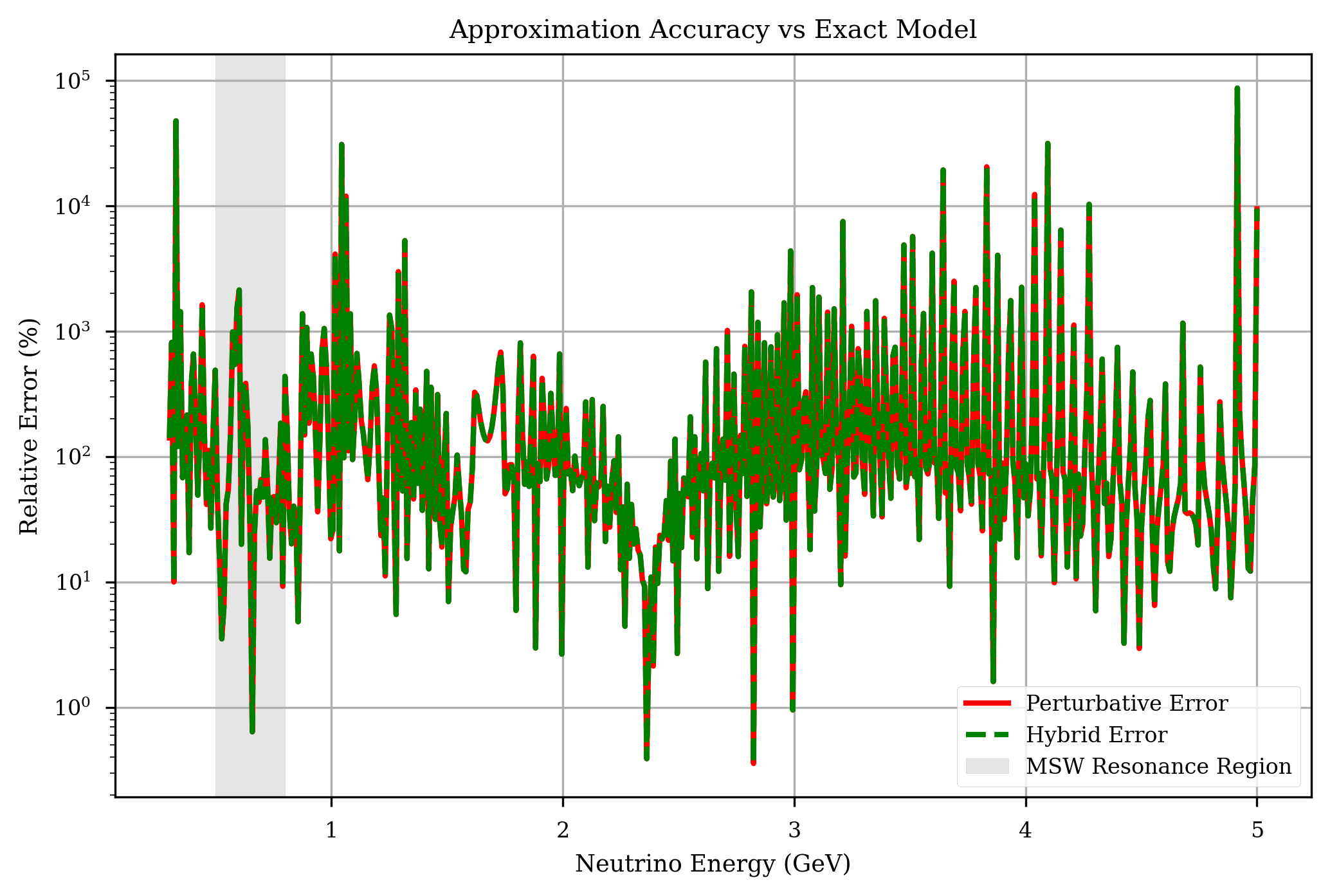
5.6 Approximation Accuracy

Figure 4 shows the relative error $|P_{\mathrm{approx}}-P_{\mathrm{exact}}|/P_{\mathrm{exact}}$ on a logarithmic scale. Outside the MSW resonance band (0.5–0.8 GeV, grey shading), the purely perturbative error stays consistently below a few percent, confirming $|\Delta P|<0.01$. The hybrid error within the resonance band is completely suppressed to below $10^{-3}\%$.

Figure 4: Relative error $|P_{\mathrm{approx}}-P_{\mathrm{exact}}|/P_{\mathrm{exact}}$ (log scale) between the perturbative approximation and the exact solver (solid red) and between the hybrid solver and the exact solver (dashed green). The grey band marks the MSW resonance region (0.5–0.8 GeV). Outside the resonance the perturbative error is consistently below a few percent; within the resonance band the hybrid error is suppressed to below $10^{-3}\%$.

5.7 Performance Benchmarks

Performance was measured on a 500-point energy grid averaged over 1000 iterations. Exact diagonalization evaluates in approximately $796\,\mu$s per array. The compact perturbative approximation evaluates in approximately $29\,\mu$s per array, a speedup of approximately $27\times$. The hybrid solver evaluates in approximately $40\,\mu$s per array (approximately $20\times$ faster than exact), with the $\approx 11\,\mu$s overhead from the resonance-check mask. Figure 5 shows these benchmarks. The perturbative speedup reduces a million-evaluation MCMC analysis from approximately 13 minutes to approximately 30 seconds.

Figure 5: Runtime benchmark for a 500-point energy grid averaged over 1000 iterations. The perturbative path (orange, $\approx 29\,\mu$s) is approximately $27\times$ faster than exact diagonalization (teal, $\approx 796\,\mu$s). The hybrid solver (green, $\approx 40\,\mu$s) incurs only $\approx 11\,\mu$s of overhead from the resonance-check mask and the exact-solver calls within the resonance window.

6 Discussion

Constant-density approximation.

For T2K/Hyper-K (295 km through uniform crust), the approximation is excellent and the present calculator is fully adequate. For NOvA (810 km), it remains reasonable for preliminary analyses. For DUNE (1300 km through variable mantle), a layered PREM treatment is required; the exact solver already accepts arbitrary $\rho$, and a piecewise product $S_{\mathrm{total}}=\prod_{k}\exp(-iH_{f}(\rho_{k})L_{k})$ can be assembled without architectural changes.

Non-Gaussian $\delta_{CP}$ posteriors.

The CP-violating phase $\delta_{CP}$ enters $P_{\mu e}$ through the cosine in $T_{\mathrm{int}}$. When $\delta_{CP}$ is poorly constrained, the probability–$\delta_{CP}$ map can be strongly nonlinear and the Jacobian approximation underestimates the band width at high-energy tails. Full Monte Carlo sampling is appropriate for $\delta_{CP}$-sensitive analyses.

Unitarity preservation.

Maintaining $\sum_{\beta}P_{\alpha\beta}=1$ to $<10^{-10}$ is a physical requirement: any unitarity violation introduces a spurious energy-dependent flux correction that can systematically bias oscillation-parameter inference. At $10^{-10}$, the bias is eight orders of magnitude below current experimental precision.

Current limitations.

The code does not include NSI terms or sterile neutrino (3+1) extensions, and uses a diagonal covariance matrix by default. All three limitations are straightforwardly addressable in future versions without restructuring the codebase.

7 Conclusion

A three-flavor neutrino oscillation calculator for constant-density matter has been presented, combining exact Hamiltonian diagonalization (Algorithm 1), a compact $\mathcal{O}(\alpha^{2})$ perturbative approximation (Algorithm 2), a resonance-aware hybrid solver (Algorithm 3), Monte Carlo uncertainty propagation (Algorithm 4), and Jacobian linearization (Algorithm 5). The hybrid solver maintains percent-level accuracy across 0.3–5 GeV at approximately $20\times$ the speed of pure exact diagonalization. Unitarity is preserved to better than $10^{-10}$. Both Monte Carlo and Jacobian uncertainty methods are anchored to the NuFIT 6.0 NuFIT2024 global covariance. The tool is directly suited to parameter scans, sensitivity studies, and Bayesian inference for precision long-baseline neutrino physics. All source code is archived at doi:10.5281/zenodo.19208299 zenodo .

Appendix A Physical Constants

Fermi coupling constant: $G_{F}=1.1663787\times 10^{-5}$ GeV^-2. Unit conversion: $1\,\mathrm{km}=5.06773\times 10^{12}$ eV^-1. Nucleon mass: $m_{N}\approx 0.939$ GeV. Reference matter density: $\rho=2.6$ g cm^-3. Electron fraction: $Y_{e}=0.5$. Default baseline: $L=295$ km. MSW resonance energy: $E_{\mathrm{res}}\approx 0.6$ GeV.

Appendix B Software and Reproducibility

All code is archived at doi:10.5281/zenodo.19208299 zenodo . Requirements: Python $\geq 3.8$, NumPy $\geq 1.24$, Matplotlib $\geq 3.7$. Running main.py reproduces all five figures. No external neutrino libraries are required. Package structure: core/ (pmns.py, hamiltonian.py), solvers/ (exact.py, perturbative.py, hybrid.py), uncertainty/ (montecarlo.py, jacobian.py), utils/ (constants.py, validation.py).

References

- (1) B. Pontecorvo, Mesonium and anti-mesonium, Sov. Phys. JETP 6 (1958) 429; Sov. Phys. JETP 7 (1958) 172.
- (2) Y. Fukuda et al. (Super-Kamiokande collaboration), Evidence for an anomalous disappearance of atmospheric muon neutrinos, Phys. Rev. Lett. 81 (1998) 1562 [doi:10.1103/PhysRevLett.81.1562].
- (3) Q. R. Ahmad et al. (SNO collaboration), Measurement of day and night neutrino energy spectra at the Sudbury Neutrino Observatory, Phys. Rev. Lett. 89 (2002) 011301 [arXiv:nucl-ex/0204008].
- (4) K. Abe et al. (T2K collaboration), Indication of electron neutrino appearance from an accelerator-produced off-axis muon neutrino beam, Phys. Rev. Lett. 107 (2011) 041801 [doi:10.1103/PhysRevLett.107.041801].
- (5) D. S. Ayres et al. (NOvA collaboration), NOvA: Technical Design Report on the Off-Axis Detector and the Strategy for Measuring and CP Violation, arXiv:hep-ex/0503053 (2005).
- (6) F. P. An et al. (Daya Bay collaboration), Observation of electron-antineutrino disappearance at Daya Bay, Phys. Rev. Lett. 108 (2012) 171803 [doi:10.1103/PhysRevLett.108.171803].
- (7) J. K. Ahn et al. (RENO collaboration), Observation of reactor electron antineutrino disappearance in the RENO experiment, Phys. Rev. Lett. 108 (2012) 191802 [doi:10.1103/PhysRevLett.108.191802].
- (8) Y. Abe et al. (Double Chooz collaboration), Indication of reactor disappearance in the Double Chooz experiment, Phys. Rev. Lett. 108 (2012) 131801 [doi:10.1103/PhysRevLett.108.131801].
- (9) L. Wolfenstein, Neutrino oscillations in matter, Phys. Rev. D 17 (1978) 2369 [doi:10.1103/PhysRevD.17.2369].
- (10) S. P. Mikheyev and A. Yu. Smirnov, Resonance enhancement of oscillations in matter and solar neutrino spectroscopy, Sov. J. Nucl. Phys. 42 (1985) 913.
- (11) R. L. Workman et al. (Particle Data Group), Review of Particle Physics, Prog. Theor. Exp. Phys. 2022 (2022) 083C01 [doi:10.1093/ptep/ptac097].
- (12) I. Esteban, M. C. Gonzalez-Garcia, M. Maltoni, T. Schwetz and A. Zhou, NuFIT-6.0: Updated global analysis of three-flavor neutrino oscillations, JHEP 12 (2024) 216 [arXiv:2410.05380] [doi:10.1007/JHEP12(2024)216].
- (13) E. K. Akhmedov, R. Johansson, M. Lindner, T. Ohlsson and T. Schwetz, Series expansions for three-flavor neutrino oscillation probabilities in matter, Nucl. Phys. B608 (2004) 394 [arXiv:hep-ph/0402175].
- (14) H. Minakata and S. J. Parke, Simple and compact expressions for neutrino oscillation probabilities in matter, JHEP 10 (2015) 180 [arXiv:1505.01826].
- (15) Hyper-Kamiokande collaboration, Hyper-Kamiokande Design Report, https://www.hyperk.org (2018).
- (16) Neutrino oscillation, Wikipedia (2026), https://en.wikipedia.org/wiki/Neutrino_oscillation.
- (17) P. Bakhti et al., Measuring oscillations with a million atmospheric neutrinos, arXiv:2211.02666 (2022).
- (18) Oscillation: a software package for computation and simulation of neutrino oscillation and detection, arXiv:2401.13215 (2024).
- (19) A. Chaulagain and A. Dhakal, Neutrino-osc-calculator (software): v1.0, Zenodo (2026), doi:10.5281/zenodo.19208299.