The Cost of Relaxation: Evaluating the Error in Convex Neural Network Verification

Abstract

Many neural network (NN) verification systems represent the network’s input-output relation as a constraint program. Sound and complete, representations involve integer constraints, for simulating the activations. Recent works convexly relax the integer constraints, improving performance, at the cost of soundness. Convex relaxations consider outputs that are unreachable by the original network. We study the worst case divergence between the original network and its convex relaxations; both qualitatively and quantitatively. The relaxations’ space forms a lattice, where the top element corresponds to a full relaxation, with every neuron linearized. The bottom element corresponds to the original network. We provide analytical upper and lower bounds for the $\ell_{\infty}$-distance between the fully relaxed and original outputs. This distance grows exponentially, w.r.t. the network’s depth, and linearly w.r.t. the input’s radius. The misclassification probability exhibits a step-like behavior, w.r.t. input radius. Our results are supported by experiments on MNIST, Fashion MNIST and random networks.

[500]Computing methodologies Neural networks [100]Computing methodologies Equation and inequality solving algorithms

1 Introduction

Artificial Intelligence, mostly driven by deep neural networks (NNs), has achieved remarkable progress in diverse domains, including recommendation systems [netflix], autonomous driving [driving], healthcare [healthcare], and large language models chat-bots [deepseek]. Despite these advances, NNs remain vulnerable to critical reliability and safety issues, such as adversarial examples [szegedy-adversarial-attacks, goodfellow-adversarial-attacks] and hallucinations in generative models [llm-halucinations]. These shortcomings raise concerns about deploying NNs in safety-critical settings, where incorrect behavior may have severe consequences [towards-vai]. Importantly, such vulnerabilities persist even in highly accurate models and often evade standard empirical defenses [athalye, raghunathan-2020]. This has led researchers to seek formal methods that provide provable guarantees regarding the safety of NN systems.

This challenge has given rise to a growing body of work on neural network verification [vnn-comp]. Formally, a verification query comes as a tuple $\tau=\langle\mathcal{P},\penalty 10000\ \langle\text{CP}(\sigma)\rangle,\mathcal{Q}\rangle$. A verification system either proves that the state $\mathcal{Q}$ is reachable by the neural network $\sigma(\cdot)$, beginning from state $\mathcal{P}$, or responds with a counter example. Usually, the neural network $\sigma(\cdot)$ is represented internally as a set of constraints $\langle\text{CP}(\sigma)\rangle$ [meng]. Depending on the type of queries they answer, verification systems are characterized as sound and/or complete. A verification system is sound, when every query that it verifies, also holds for the original network. Symmetrically, a verification system is complete when every query, that holds for the original network, is also verified [meng]. The soundness or completeness of a verification largely depends on the choice of the internal representation $\langle\text{CP}(\sigma)\rangle$, as the latter describes the NN’s input-output (IO) relation. An over-approximation of the IO-relation verifies states that are unreachable from the original network, thus leading to unsoundness. However, under-approximating the IO-relation fails to verify states that are reachable from the true network.

One popular technique for representing the NN’s IO-relation is mixed integer linear programming (MILP) [meng]. This involves expressing the NN’s behavior as a set of linear inequalities on real or integer variables. The use of integer variables is essential for exactly describing the non-linearity introduced by the activation functions. MILP leads to sound and complete verification, and has been successfully employed by a variety of systems, e.g. [marabou, marabou-2]. However, this precision comes at the cost of performance, since the NN verification problem is intractable [katz].

In parallel to sound and complete verification alternative approaches are proposed, relaxing the verification problem, thus improving on performance. In particular, here we focus on a popular technique for complete, but unsound, verification, via convex relaxations. There the NN’s IO-relation is described as a convex (linear) program, involving only linear constraints on real variables [ehlers]. Typically this involves the computation of pre-activation interval bounds for each neuron in the network, using interval bound propagation (IBP) [gowal]. Since we now only have linear, real constraints the program can be solved in polynomial time [elipsoid-method]. Additionally, numerical methods can be employed, further improving efficiency [wong, liu, li, kabahala]. This approach has been applied in adversarial robustness certification [wong, liu, li, kabahala]. Finally, a linear objective is employed to keep the relaxation close to the original network [wong, liu, li, kabahala].

The above methods avoid the computational cost, by relaxing the integer constraints involved in a MILP. However, this non-linearity is essential to a NN’s expressive power. Thus, relaxations hinder a NN’s expressivity [lederer, minsky-1969]. In this work, we are interested to evaluate the cost of convex relaxations have to a verification system’s precision.

Related work in [salman-2019] studies the consequences convex relaxations have to robustness certification queries. They present a novel framework which characterizes a family of convex relaxations including popular approaches, such as [wong, crown]. They prove that the certification quality of each relaxation in the family cannot exceed a certain optimal barrier. Moreover, their extensive experimental results suggest that this barrier has already reached by existing methods. Thus, conclude that further research will not provide significant improvements. Despite their insights, some details where not included in their examination. Their work primarily focuses on robustness certification, not examining the consequences of convex relaxations in other verification settings. Moreover, they concentrate on “static” real-word networks, not exploring the correlation of the relaxation error with other network parameters.

Our work aims to cover the above gaps. We examine a fundamental reachability query. Since NNs are functions, a given input, completely determines their output. However, this does not hold for convexly relaxed representations of NNs. There, an input specifies a set of possible outcomes, including the original network’s output. This work aims to evaluate the degree of error introduced by choosing a relaxed output, instead of computing the true value. We answer this question both qualitatively and quantitatively. First, we explore the space of the feasible convex relaxations, observing its lattice structure. The lattice’s top element corresponds to the fully relaxed convex solution, where every neuron is linearized. The lattice’s bottom element corresponds to the original network. We remark that a fully relaxed NN corresponds to the strictly weaker learning paradigm of a linear model. Subsequently, we proceed on evaluating the difference between the fully relaxed and original output. We present analytical upper and lower bounds for their $\ell_{\infty}$-distance. Further we experimentally, test the correlation of the fully relaxed and original distance, w.r.t. the network’s depth and input radius. We observe an exponential growth to the $\ell_{\infty}$-distance, w.r.t. the network’s depth, while a linear growth, w.r.t. the input radius. Additionally, we test how this divergence affects classification problems, by estimating the misclassification probability. We observe that the misclassification probability follows a step-like behavior, w.r.t. the input radius.

Contributions. This paper includes the following contributions:

1. We characterize the space of convex relaxations for a particular ReLU-NN. For relaxations choosable by a linear objective, we observe a lattice structure in the solution space (Theorem˜3.1). The lattice’s top element corresponding to a fully relaxed, linear network, while the bottom element to the original network. We explore the structural differences between the fully relaxed convex solution, where every neuron is linearized and the original network. We remark their expressive difference.

2. We quantify the difference between the fully relaxed and the original network. We measure the $\ell_{\infty}$-distance between the relaxed and original outputs, where we provide analytical lower (Theorem˜4.1) and upper (Theorem˜4.4) bounds. Our analytical expressions highlight an exponential dependence from the network’s depth. This dependence becomes also evident from experiments on 30 random networks with increasing depths.

3. The computation of a convex relaxation is initialized w.r.t. a vicinity of the input space. We examine how this vicinity’s radius affects the quality of the relaxation. We perform experiments on real-life MNIST and Fashion MNIST networks. There, we observe a linear dependence of the $\ell_{\infty}$-distance, between the relaxed and original outputs, w.r.t. the input vicinity’s radius. In the same setting, we examine how relaxations affect classification. We observe a step-like behavior of the misclassification probability, w.r.t. the input vicinity’s radius. For both networks the misclassification probability approaches 1, when half of the input space is considered for the relaxation.

Outline. We begin in Section˜2 presenting some preliminary notions, rigorously defining ReLU-NN, and the Interval Bound Propagation method. Subsequently, in Section˜3 we explore the connection between NN verification and various constraint formulations. In particular, we discuss MILP and convex relaxations, followed by analysis on the solution space of convex relaxations. We focus on the top relaxation, where every neuron is convexly relaxed. In Section˜4 we discuss various error metrics. We rigorously define the worst case relaxation error, proving upper and lower bounds. We supplement our theoretical analysis, with experiments in Section˜5. Finally, we conclude in Section˜6.

2 Preliminaries

For any natural number $d\in\mathbb{N}$, $[d]$ denotes the set $[d]=\{1,2,\dots,d\}$. Vectors in $\mathbb{R}^{d}$ are denoted by bold, e.g., $\mathbf{x}$, with coordinates $x_{i}$, $i\in[d]$, while scalar values by light, e.g., $x$. The vectors $\mathbf{0}$ and $\mathbf{1}$ denote the all-zeros and all-ones vectors, respectively. For $i\in[d]$, $\mathbf{e}^{i}$ denotes the $i$-th canonical base vector. For a vector $\mathbf{x}\in\mathbb{R}^{d}$, $\|\mathbf{x}\|_{p}$ denotes its $\ell_{p}$–norm. We are particularly interested in $\ell_{\infty}$–norm, where $\|\mathbf{x}\|_{\infty}=\max_{i\in[d]}|x_{i}|$. Finally, for $\rho>0$, $\mathcal{B}_{p}(\mathbf{x}_{o},\rho)$ denotes the $\ell_{p}$–sphere, centered at $\mathbf{x}_{o}$, with radius $\rho$, w.r.t. the $\ell_{p}$–norm. Namely, $\mathcal{B}_{p}(\mathbf{x}_{o},\rho)=\{\mathbf{x}\in\mathbb{R}^{d}\mid\|\mathbf{x}_{o}-\mathbf{x}\|\leq\rho\}$. We extend real-valued operations to vectors in a coordinate-wise manner. For two vectors $\mathbf{x},\mathbf{y}\in\mathbb{R}^{d}$, $\mathbf{x}\odot\mathbf{y}$ denotes their coordinate-wise product. For $\mathbf{x}\in\mathbb{R}^{d}$, $|\mathbf{x}|$ denotes the vector $|\mathbf{x}|=(|x_{1}|,\dots,|x_{d}|)$. Additionally, $\mathbf{x}_{+}$ denotes the positive part, while $\mathbf{x}_{-}$ the negative part of a vector. For two vectors $\mathbf{x},\mathbf{y}\in\mathbb{R}^{d}$, $\mathbf{m}=\max\{\mathbf{x},\mathbf{y}\}$ denotes the coordinate-wise maximum, i.e. $m_{i}=\max\{x_{i},y_{i}\}$, for every $i\in[d]$. Matrices $A\in\mathbb{R}^{d_{1}\times d_{2}}$ are denoted with capital letters. For a matrix $A\in\mathbb{R}^{d_{1}\times d_{2}}$ its transpose is denoted by $A^{T}\in\mathbb{R}^{d_{2}\times d_{1}}$. Additionally, $\mathbf{O}$ denotes the all zero matrix. The vector conventions are also applied to matrices.

Comparison $\mathbf{x}\leq\mathbf{y}$, for two vectors $\mathbf{x},\mathbf{y}\in\mathbb{R}^{d}$ should be understood coordinate-wise. Namely, the comparison $\mathbf{x}\leq\mathbf{y}$ holds if and only if $x_{i}\leq y_{i}$, for every $i\in[d]$. We extend real interval to multidimensional spaces. In particular, let $I=[\mathbf{\boldsymbol{\ell}},\boldsymbol{u}]\subseteq\mathbb{R}^{d}$ denote the set of points $\mathbf{x}\in\mathbb{R}^{d}$, s.t. $\boldsymbol{\ell}\leq\mathbf{x}\leq\boldsymbol{u}$. Geometrically, multidimensional intervals correspond to axis-aligned, hyper-rectangles. For a real function $f\colon\mathbb{R}\to\mathbb{R}$, we implicitly use $\mathbf{f}(\cdot)$ to denote the function $\mathbf{f}\colon\mathbb{R}^{d}\to\mathbb{R}^{d}$, where $\mathbf{f}(\mathbf{x})=(f(x_{1}),f(x_{2}),\dots,f(x_{d}))$. Subsequently, we use extensively linear functions of the form $\mathbf{f}(\mathbf{x})=W\mathbf{x}+\mathbf{b}$, where $\mathbf{f}\colon\mathbb{R}^{{d_{\text{in}}}}\to\mathbb{R}^{d_{\text{out}}}$, $W\in\mathbb{R}^{d_{\text{out}}\times{d_{\text{in}}}}$, and $\mathbf{b}\in\mathbb{R}^{d_{\text{out}}}$.

2.1 Neural Networks

We view neural networks as functions between two sets. In particular, we denote the inputs or feature space by $\mathbb{F}$. Moreover, we denote the outputs or score space by $\mathbb{S}$. A neural network simply maps feature points to scores. This is achieved by passing the features point through a sequence of “semi-linear” layers. In each layer, the linearity is disrupted by an activation function. This enables neural networks to have a sophisticated emergent behavior. We give the following formal definition.

Definition 2.1 (Neural Network).

Let $L\in\mathbb{N}$ denote the number of layers (or depth). Moreover, let $D$ denote the network’s architecture, i.e. a sequence of $L+1$ natural numbers, where ${d_{\text{in}}}=d_{0},d_{1},\dots,d_{L-1},d_{L}=d_{\text{out}}$. Additionally, let $W$ denote a sequence of $L$ real matrices, s.t. $W^{(i)}\in\mathbb{R}^{d_{i}\times d_{i-1}}$, for each $i\in[L]$. Furthermore, $\beta$ denotes a sequence of $L$ real vectors, s.t. $\mathbf{b}^{(i)}\in\mathbb{R}^{d_{i}}$, for each $i\in[L]$. Finally, $\alpha$ denotes a sequence of $L$ activation functions, s.t. $\mathbf{a}^{(i)}\colon\mathbb{R}^{d_{i}}\to\mathbb{R}^{d_{i}}$, for every $i\in[L]$. A neural network (NN) $\sigma\colon\mathbb{F}\to\mathbb{S}$, with $\mathbb{F}\subset\mathbb{R}^{{d_{\text{in}}}},\mathbb{S}\subset\mathbb{R}^{d_{\text{out}}}$. is described as the tuple $\sigma=\langle L,D,W,\beta,\alpha\rangle$. For an input $\mathbf{x}\in\mathbb{F}$, the value of $\sigma(\mathbf{x})$ is given as the value $\sigma^{(L)}$ in the system of recursive equations below.

$$\left.\begin{array}[]{ll}\sigma^{(0)}&=\mathbf{x}\\ \sigma^{(i)}&=\mathbf{a}^{(i)}[W^{(i)}\sigma^{(i-1)}+\mathbf{b}^{(i)}],\quad\forall i\in[L]\end{array}\right\}$$ (1)

We focus on the Rectified Linear Unit (ReLU) activation function. Given a vector $\mathbf{x}$, let $\mathbf{r}(\mathbf{x})$ denote the vector $\max\{\mathbf{x},\mathbf{0}\}$, where the maximum is taken coordinate-wise.

In many applications, we need to map inputs to a finite set of labels, or classes. We do this by assigning to the input the class with the highest score. Formally, let $\mathcal{C}\subset\mathbb{N}$ be a finite set of classes, with $|\mathcal{C}|=d_{\text{out}}$. A classifier $\kappa\colon\mathbb{F}\to\mathcal{C}$ is constructed with respect to the NN $\sigma(\cdot)$, as $\kappa(\mathbf{x})=\arg\max_{i\in[d_{\text{out}}]}\sigma_{i}(\mathbf{x})$.

2.2 Interval Bound Propagation

Figure 1: From left to right: The input domain $[-1,1]^{2}$ (blue). The pre-activation polytope (blue). The post-activation polytope (red). For the pre- and post- activation polytopes, we also depict their interval bounds (grey). The figures are drawn for a single layer network, with parameters $W=\left[\begin{array}[]{cc}1&2\\ 3&-4\end{array}\right]$ and $\mathbf{b}=[-1\penalty 10000\ \penalty 10000\ 1]^{T}$. All the points of the pre-activation polytope with non-positive $x$-values are projected to the $y$-axis. Similarly, the points with non-positive $y$-values are projected to the $x$-axis. Finally, all points of the pre-activation polytope with both non-positive coordinates are projected to the axes’ origins. The pre-activation bound is $I=[\boldsymbol{\ell},\boldsymbol{u}]$, where $\boldsymbol{\ell}=[-5\penalty 10000\ -5]^{T}$ and $\boldsymbol{u}=[3\penalty 10000\ 7]^{T}$. The post-activation bound $\widehat{I}=[\widehat{\boldsymbol{\ell}},\widehat{\boldsymbol{u}}]$, where $\boldsymbol{\ell}=\mathbf{0}$ and $\widehat{\boldsymbol{u}}=\boldsymbol{u}$.

Consider a network $\sigma=\langle L,D,W,\beta,\alpha\rangle$, where $\alpha$ denotes a sequence of $L$ increasing activation functions of the form $\mathbf{a}^{(i)}\colon\mathbb{R}^{d_{i}}\to\mathbb{R}^{d_{i}}$. Let $\widehat{I}^{(0)}=[\boldsymbol{\ell},\boldsymbol{u}]$ be an interval in the input space $\mathbb{F}$. For each layer $i\in[L]$, we call pre-activation bound $I^{(i)}$ the minimum interval that bounds the output of the layer’s linear part, i.e. the layer’s value before the activation is applied. For the $i$-th layer, the post-activation bound $\widehat{I}^{(i)}$ is the minimum interval that bounds the output of the layer’s activation. Thus, we derive two sequences $\{I^{(i)}\}_{i\in[L]}$, $\{\widehat{I}^{(i)}\}_{i\in[L]}$ of the pre- and post- activation bounds, respectively. Here we briefly review the Interval Bound Propagation (IBP) method [gowal], for computing the pre- and post- activation bounds.

For each layer $i\in[L]$, we can decompose its weight matrix $W^{(i)}$ into its positive $W^{(i)}_{+}\geq\mathbf{O}$ and negative $W^{(i)}_{-}\leq\mathbf{O}$ components, s.t. $W^{(i)}=W^{(i)}_{+}+W^{(i)}_{-}$. Now the pre- and post- activation bounds can be computed recursively, using Equation˜2. The method’s correctness is established in Proposition˜2.2. Finally, IBP on a single layer is illustrated in Figure˜1.

$$\hskip-21.33955pt\begin{array}[]{l}I^{(i+1)}=\begin{cases}\boldsymbol{\ell}^{(i+1)}=W^{(i+1)}_{+}\widehat{\boldsymbol{\ell}}^{(i)}+W^{(i+1)}_{+}\widehat{\boldsymbol{u}}^{(i)}+\mathbf{b}^{(i+1)}\\ \boldsymbol{u}^{(i+1)}=W^{(i+1)}_{-}\widehat{\boldsymbol{u}}^{(i)}+W^{(i+1)}_{-}\widehat{\boldsymbol{\ell}}^{(i)}+\mathbf{b}^{(i+1)}\end{cases}\hskip-7.11317pt\widehat{I}^{(i+1)}=\begin{cases}\widehat{\boldsymbol{\ell}}^{(i+1)}=\mathbf{a}^{(i+1)}(\boldsymbol{\ell}^{(i+1)})\\ \widehat{\boldsymbol{u}}^{(i+1)}=\mathbf{a}^{(i+1)}(\boldsymbol{u}^{(i+1)})\end{cases}\end{array}\hskip-42.67912pt$$ (2)

Proposition 2.2.

Consider $\sigma=\langle L,D,W,\beta,\alpha\rangle$, where $\alpha$ denotes a sequence of increasing activation functions. Now, let $\{I^{(i)}\}_{i\in[L]}$ and $\{\widehat{I}^{(i)}\}_{i\in[L]}$ be the sequence of pre- and post- activation bounds generated by the IBP, for an input interval $\widehat{I}^{(0)}$. Then $\widehat{I}^{(L)}$ is the minimum interval, s.t. $\sigma(\widehat{I}^{(0)})\subseteq\widehat{I}^{(L)}$, w.r.t. set inclusion.

3 Verification as Constraint Programming

In this section, we explore the connections between various constraint-based formulations and NN verification. Recall, a verification instance is described by a query $\tau=\langle\mathcal{P}(\mathbf{x}),\langle\sigma\rangle(\mathbf{x},\mathbf{y}),\mathcal{Q}(\mathbf{y})\rangle$. A verification system, answers a reachability query. Namely, if for every input $\mathbf{x}$, satisfying the pre-condition $\mathcal{P}(\mathbf{x})$, every output $\mathbf{y}$, reachable from $\mathbf{x}$ by the NN $\sigma(\cdot)$, satisfies the post-condition $\mathcal{Q}(\mathbf{y})$. This is captured by the problem of satisfying the first-order formula $(\forall\mathbf{x}\penalty 10000\ \forall\mathbf{y})\penalty 10000\ [\mathcal{P}(\mathbf{x})\land\langle\sigma\rangle(\mathbf{x},\mathbf{y})\to\mathcal{Q}(\mathbf{y})]$. Otherwise, the verification system returns a counterexample, as a pair $\mathbf{x},\mathbf{y}$, s.t. $\mathbf{x},\mathbf{y}\models\mathcal{P}(\mathbf{x})\land\langle\sigma\rangle(\mathbf{x},\mathbf{y})\lor\lnot\mathcal{Q}(\mathbf{y})$.

Above, $\langle\sigma\rangle(\mathbf{x}.\mathbf{y})$ denotes the IO-relationship of a fixed neural network $\sigma(\cdot)$. However, directly applying the recursive definition of Equation˜1 is not suitable for efficient reasoning. In the literature, a NN $\sigma(\cdot)$ is often described by a set of constraints $\text{CP}(\sigma)$. Let $\langle\text{CP}(\sigma)\rangle(\mathbf{x},\mathbf{y})$ denote the IO-relationship of the constraint program $\text{CP}(\sigma)$. If $\langle\text{CP}(\sigma)\rangle(\mathbf{x},\mathbf{y})\supseteq\langle\sigma\rangle(\mathbf{x},\mathbf{y})$, we call the formalism $\text{CP}(\sigma)$ complete. Symmetrically, we call the formalism $\text{CP}(\sigma)$ sound if $\langle\text{CP}(\sigma)\rangle(\mathbf{x},\mathbf{y})\subseteq\langle\sigma\rangle(\mathbf{x},\mathbf{y})$. Naturally, the choice of formalism directly affects the behavior of a verification system. A complete, but unsound formalism leads to verification of queries $\tau$, that do not hold for the true network $\sigma(\cdot)$. On the other hand, a sound but incomplete formalism will fail to verify queries $\tau$ that hold for $\sigma(\cdot)$.

We examine two such formalisms, widely used in the literature. The sound and complete MILP, and its complete, but unsound convex relaxation. We focus on an fundamental reachability query. For a fixed input $\mathbf{x}_{o}$, how far apart can be the outputs $\mathbf{y}_{o}$, w.r.t. each formalism. We give a qualitative view of the problem, highlighting the structural differences.

3.1 The Sound and Complete MILP Formalization

One popular way to implement a sound and complete verification system is to express a given ReLU-NN as a mixed integer linear program (MILP). This results in expressing the given network as a set of linear constraints, involving both integer and real variables. Subsequently, we call integer constraints the constraints that include discrete variables. In Equation˜3 below, we present the description of a ReLU-NN as a MILP.

$$\left.\begin{array}[]{l l l}\widehat{\boldsymbol{\sigma}}^{(0)}&=\mathbf{x}\\ \mathbf{y}&=\widehat{\boldsymbol{\sigma}}^{(L)}\\ \\ \boldsymbol{\sigma}^{(i)}&=W^{(i)}\widehat{\boldsymbol{\sigma}}^{(i-1)}+\mathbf{b}^{(i)},&\forall i\in[L]\\ \widehat{\boldsymbol{\sigma}}^{(i)}&\geq\boldsymbol{\sigma}^{(i)},&\forall i\in[L]\\ \widehat{\boldsymbol{\sigma}}^{(i)}&\geq\mathbf{0},&\forall i\in[L]\\ \\ \widehat{\boldsymbol{\sigma}}^{(i)}&\leq\boldsymbol{\sigma}^{(i)}+M\mathbf{t}^{(i)},&\forall i\in[L]\\ \widehat{\boldsymbol{\sigma}}^{(i)}&\leq M(\mathbf{1}-\mathbf{t}^{(i)}),&\forall i\in[L]\\ \\ \lx@intercol\mathbf{t}^{(i)}\in\{0,1\}^{d^{i}_{\text{out}}},\hfil\lx@intercol&\forall i\in[L]\\ \lx@intercol\boldsymbol{\sigma}^{(i)},\widehat{\boldsymbol{\sigma}}^{(i)}\in\mathbb{R}^{d^{i}_{\text{out}}},\hfil\lx@intercol&\forall i\in[L]\\ \lx@intercol\mathbf{x}\in\mathbb{R}^{d_{\text{in}}},\penalty 10000\ \mathbf{y}\in\mathbb{R}^{d_{\text{out}}}\hfil\lx@intercol\\ \end{array}\right\}$$ (3)

Above, for the $j$-th neuron of the $i$-th layer we distinguish between its pre-activation value $\sigma^{(i)}_{j}$ and its post-activation value $\widehat{\sigma}^{(i)}_{j}$. The constant $M$ represents an arbitrarily high value. The integer vector $\mathbf{t}$ models the behavior of the ReLU activation. For the $j$-th neuron of the $i$-th layer, $t^{(i+1)}_{j}=0$ iff $\widehat{\sigma}^{(i+1)}_{j}=\sigma^{(i+1)}_{j}$, i.e., ReLU is activated; otherwise, $t^{(i+1)}_{j}=1$.

For a given ReLU-NN $\sigma(\cdot)$, we denote the mixed-integer linear program of Equation˜3 by $\textsc{Milp}(\sigma)$. Additionally, let $\textsc{Milp}(\sigma)|_{\mathbf{x}=\mathbf{x}_{o}}$ denote the set of solutions of the MILP, for a fixed input $\mathbf{x}=\mathbf{x}_{o}$. Observe that $\textsc{Milp}(\sigma)|_{\mathbf{x}=\mathbf{x}_{o}}$ is a singleton. In other words, for a given input, we have a unique solution. Thus, the MILP formalism results is sound and complete.

3.2 Completeness with Convex Relaxations

Unfortunately, the appealing theoretical properties of MILP formulation comes at the cost of performance [katz]. Due to the involvement of integer constraints, solving the system of Equation˜3 is intractable [conforti-IP]. To circumvent this, some approaches use convex relaxations [wong]. They replace the integer constraints of Equation˜3, with their convex relaxations.

To achieve this, we assume the pre-activation bounds, as derived from IBP [gowal]. Consider an interval $I_{o}\subseteq\mathbb{F}$. For the $i$-th layer, the pre-activation bound is the interval $I^{(i)}$, s.t. $\sigma^{(i)}\in I^{(i)}$, for any $\mathbf{x}\in I_{o}$. For $I^{(i)}=[\boldsymbol{\ell}^{(i)},\boldsymbol{u}^{(i)}]$, with $\boldsymbol{\ell}\leq\mathbf{0}\leq\boldsymbol{u}$, we define the vector $\mathbf{q}^{(i)}\in[\mathbf{0},\mathbf{1}]$, s.t.

$$\mathbf{q}^{(i)}=\frac{\boldsymbol{u}^{(i)}}{\boldsymbol{u}^{(i)}-\boldsymbol{\ell}^{(i)}}.$$ (4)

Then, the integer constraints are replaced with $\widehat{\boldsymbol{\sigma}}^{(i)}\leq\mathbf{q}^{(i)}\odot(\boldsymbol{\sigma}^{(i)}-\boldsymbol{\ell}^{(i)})$. Thus, resulting to the convex program bellow.

$$\left.\begin{array}[]{l l l}\widehat{\boldsymbol{\sigma}}^{(0)}&=\mathbf{x}\\ \mathbf{y}&=\widehat{\boldsymbol{\sigma}}^{(L)}\\ \\ \boldsymbol{\sigma}^{(i)}&=W^{(i)}\widehat{\boldsymbol{\sigma}}^{(i-1)}+\mathbf{b}^{(i)},&\forall i\in[L]\\ \widehat{\boldsymbol{\sigma}}^{(i)}&\geq\boldsymbol{\sigma}^{(i)},&\forall i\in[L]\\ \widehat{\boldsymbol{\sigma}}^{(i)}&\geq\mathbf{0},&\forall i\in[L]\\ \\ \widehat{\boldsymbol{\sigma}}^{(i)}&\leq\mathbf{q}^{i}\odot(\boldsymbol{\sigma}^{(i)}-\boldsymbol{\ell}^{(i)}),&\forall i\in[L]\\ \\ \lx@intercol\boldsymbol{\sigma}^{(i)},\widehat{\boldsymbol{\sigma}}^{(i)}\in\mathbb{R}^{d^{i}_{\text{out}}},\hfil\lx@intercol&\forall i\in[L]\\ \lx@intercol\mathbf{x}\in\mathbb{R}^{d_{\text{in}}},\penalty 10000\ \mathbf{y}\in\mathbb{R}^{d_{\text{out}}}\hfil\lx@intercol\\ \end{array}\right\}$$ (5)

We denote the convex program of Equation˜5 by $\textsc{Conv}(\sigma)$. For a given input $\mathbf{x}_{o}$, the set of solutions to this program is denoted by $\textsc{Conv}(\sigma)|_{\mathbf{x}=\mathbf{x}_{o}}$. Notably, the set $\textsc{Conv}(\sigma)|_{\mathbf{x}=\mathbf{x}_{o}}$ contains multiple solutions, including the MILP solution, i.e.,

$$\textsc{Conv}(\sigma)|_{\mathbf{x}=\mathbf{x}_{o}}\supseteq\textsc{Milp}(\sigma)|_{\mathbf{x}=\mathbf{x}_{o}}=\{\sigma(\mathbf{x}_{o})\}.$$ (6)

Finally, due to the soundness and completeness of the MILP formulation, we know that Equation˜3 has a unique solution, for a given input $\mathbf{x}_{o}$, namely $\mathbf{y}_{o}=\sigma(\mathbf{x}_{o})$.

3.3 Optimization & Adversarial Robustness

In many applications [wong, liu, li, kabahala, salman-2019], we want to optimize an objective function over the feasible NN states. In particular, assume a linear objective function of the form $\xi([\boldsymbol{\sigma}\penalty 10000\ \penalty 10000\ \widehat{\boldsymbol{\sigma}}])=\mathbf{c}^{T}[\boldsymbol{\sigma}\penalty 10000\ \penalty 10000\ \widehat{\boldsymbol{\sigma}}]+c_{0}$, where the vector $[\boldsymbol{\sigma}\penalty 10000\ \penalty 10000\ \widehat{\boldsymbol{\sigma}}]$ is composed of all the variables in $\textsc{Milp}(\sigma)$ and $\textsc{Conv}(\sigma)$. Let $\textsc{CP}\in\{\textsc{Milp},\penalty 10000\ \textsc{Conv}\}$. We consider the following optimization problem,

$$\xi^{\ast}=\max\{\xi([\boldsymbol{\sigma}\penalty 10000\ \penalty 10000\ \widehat{\boldsymbol{\sigma}}])\mid\boldsymbol{\sigma},\widehat{\boldsymbol{\sigma}}\in\textsc{CP}(\sigma)\}.$$ (7)

A particular instance of the above optimization problem includes adversarial robustness [goodfellow-adversarial-attacks, wong, salman-2019]. In adversarial robustness we are interested in examining if a given area is free of adversarial examples. In particular, assume a point $\mathbf{x}_{o}$, and an interval $I_{o}$, s.t. $\mathbf{x}_{o}\in I_{o}$. Is every input in $I_{o}$ assigned to the same class $j_{o}=\kappa(\mathbf{x}_{o})$ of $\mathbf{x}_{o}$? We can certify the robustness of the network in the vicinity $I_{o}$, by defining a certain linear cost function. In particular, let

$$\xi([\boldsymbol{\sigma}\penalty 10000\ \penalty 10000\ \widehat{\boldsymbol{\sigma}}])=w^{(L)}_{j}\widehat{\boldsymbol{\sigma}}^{(L)}-w^{(L)}_{j_{o}}\widehat{\boldsymbol{\sigma}}^{(L)}.$$ (8)

for some $j\neq j_{o}$. If the optimization problem (7) with the objective function of Equation˜8 yields a positive solution, then there is an adversarial example in $I_{o}$. If the optimization problem yields a negative solution for every $j\neq j_{o}$, then the vicinity $I_{o}$ is robust.

Note that the choice of the CP formulation matters. In particular, since $\textsc{Conv}(\sigma)|_{\mathbf{x}=\mathbf{x}_{o}}\supseteq\textsc{Milp}(\sigma)|_{\mathbf{x}=\mathbf{x}_{o}}$, we have $\textsc{Conv}(\sigma)|_{\mathbf{x}\in I_{o}}\supseteq\textsc{Milp}(\sigma)|_{\mathbf{x}\in I_{o}}$. Intuitively, this entails that fewer and smaller vicinities $I_{o}$ will be certified as robust by the convex relaxation [wong, salman-2019]. However, every robustly certifiable vicinity $I_{o}$, by the convex relaxation, will also be robustly certified by the original MILP [wong].

3.4 The Solutions Space of the Convex Relaxation

Figure 2: (Top) The lattice-structured space of feasible convex relaxations, that are choosable by a linear objective function $V(\Lambda)$. (Bottom) The relaxation of $V(\Lambda)$, for the single-layer network of Figure˜1. For the layer’s two neurons, holds $\mathbf{q}^{T}=[0.37\penalty 10000\ 0.58]$. From left to right. $\lambda_{1}=0,\lambda_{2}=0$, thus $\widehat{\sigma}_{1},\widehat{\sigma}_{2}$ is exact. $\lambda_{1}=0,\lambda_{2}=1$, thus $\widehat{\sigma}_{1}$ is exact and $\widehat{\sigma}_{2}$ is linearized. $\lambda_{1}=1,\lambda_{2}=0$, thus $\widehat{\sigma}_{1}$ is linearized and $\widehat{\sigma}_{2}$ is exact. Finally, $\lambda_{1}=\lambda_{2}=1$, where the network is fully relaxed.

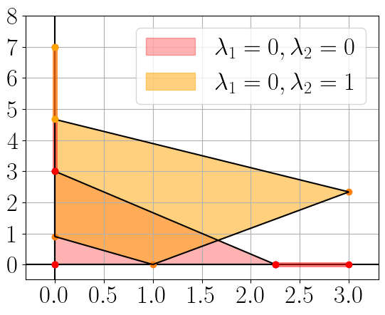
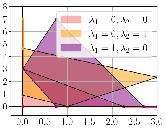
Here we discuss the structure of the solutions space $\textsc{Conv}(\sigma)|_{\mathbf{x}=\mathbf{x}_{o}}$. Firstly, we observe that this space is innumerable, but bounded, and isomorphic to a hypercube. However, only the vertices of the hypercube are eligible to be chosen by a linear objective. This drastically reduces the number of relevant feasible solutions to a finite set. Moreover, the vertices of the hypercube exhibit an interesting lattice-structure. The top element of the lattice corresponds to the fully-relaxed convex solution, where every neuron is linearized. The bottom element of the lattice corresponds to the original network, where no neuron is relaxed. For each element between the top and bottom, we have an intermediate case, where only a portion of the total number of neurons is linearly relaxed. This lattice is presented in Figure˜2.

We characterize the family of solutions in $\textsc{Conv}(\sigma)|_{\mathbf{x}=\mathbf{x}_{o}}$. Each solution will correspond to a vector $\boldsymbol{\lambda}\in[0,1]^{\Delta}$, s.t. $\Delta=\sum_{i\in[d]}d^{i}_{\text{in}}+d^{L}_{\text{out}}$. Intuitively, the dimension $\Delta$ corresponds to the number of neurons in the network. Let $\lambda^{(i)}_{j}$ be the coordinate of the $\boldsymbol{\lambda}$ vector, corresponding to the $j$-th neuron of the $i$-th layer. When the neuron is linearly relaxed, we have $\lambda^{(i)}_{j}=1$. Otherwise, it holds $\lambda^{(i)}_{j}=0$. Formally, we define $\lambda^{(i)}_{j}$ as the following ratio:

$$\lambda^{(i)}_{j}=\frac{\widehat{\sigma}^{(i)}_{j}\cdot(\widehat{\sigma}^{(i)}_{j}-\sigma^{(i)}_{j})}{q^{(i)}_{j}\cdot(\sigma^{(i)}_{j}-\ell^{(i)}_{j})}.$$ (9)

Let $\Lambda=[0,1]^{\Delta}$, be set including all possible vectors $\boldsymbol{\lambda}$. Observe that $\Lambda$ is a $\Delta$-dimensional hypercube; isomorphic to $\textsc{Conv}(\sigma)|_{\mathbf{x}=\mathbf{x}_{o}}$. Namely, every $\boldsymbol{\lambda}\in\Lambda$ uniquely determines a sequence of feasible solutions $[\boldsymbol{\sigma}\penalty 10000\ \penalty 10000\ \widehat{\boldsymbol{\sigma}}]\in\textsc{Conv}(\sigma)|_{\mathbf{x}=\mathbf{x}_{o}}$, and vice versa.

Theorem 3.1.

Consider any linear objective of the form $\xi([\boldsymbol{\sigma}\penalty 10000\ \penalty 10000\ \widehat{\boldsymbol{\sigma}}])=\mathbf{c}^{T}[\boldsymbol{\sigma}\penalty 10000\ \penalty 10000\ \widehat{\boldsymbol{\sigma}}]+c_{0}$, where $[\boldsymbol{\sigma}\penalty 10000\ \penalty 10000\ \widehat{\boldsymbol{\sigma}}]\in\textsc{Conv}(\sigma)|_{\mathbf{x}=\mathbf{x}_{o}}$. Let $[\boldsymbol{\sigma}\penalty 10000\ \penalty 10000\ \widehat{\boldsymbol{\sigma}}]^{\ast}$ be the optimal solution w.r.t. $\xi(\cdot)$, and $\boldsymbol{\lambda}^{\ast}\in\Lambda$ its corresponding ratios vector. Then, $\boldsymbol{\lambda}^{\ast}$ is a vertex of $\Lambda$, i.e. $\boldsymbol{\lambda}^{\ast}\in V(\Lambda)=\{0,1\}^{\Delta}$.

Theorem˜3.1 radically reduces the number of relevant convex solutions. From the innumerable hypercube $\Lambda$, to the finite set of vertices $V(\Lambda)$. Moreover, the vertices $V(\Lambda)$ form a lattice, with $\max,\min$ as its join and meet operations. For the top element of this lattice, we have $\boldsymbol{\lambda}=\mathbf{1}$, corresponding to the fully relaxed network. For its bottom element, we have $\boldsymbol{\lambda}=\mathbf{0}$ corresponding to the original network. For the single layer network of Figure˜1, we present all the relaxations in $V(\Lambda)$ in Figure˜2. However, note that, in general the hypercube $\Lambda$ has an exponential number of vertices, w.r.t. the number of neurons $\Delta$.

3.5 The Top Convex Relaxation

We conclude this section by discussing the top element of the $V(\Lambda)$ lattice. Recall that this solution of Equation˜5 corresponds to the case where every neuron relaxed. Interestingly, this results into degenerating the NN into a single layer. Thus, drastically reducing the its expressivity [minsky-1969, lederer]. To that end, we rewrite the CP of Equation˜5 as follows.

$$\left.\begin{array}[]{l l l}\widehat{\boldsymbol{\sigma}}^{(0)}&=\mathbf{x}\\ \mathbf{y}&=\widehat{\boldsymbol{\sigma}}^{(L)}\\ \\ \boldsymbol{\sigma}^{(i)}&=W^{(i)}\widehat{\boldsymbol{\sigma}}^{(i-1)}+\mathbf{b}^{(i)},&\forall i\in[L]\\ \widehat{\boldsymbol{\sigma}}^{(i)}&=\mathbf{q}^{(i)}\odot(\boldsymbol{\sigma}^{(i)}-\boldsymbol{\ell}^{(i)}),&\forall i\in[L]\\ \\ \lx@intercol\boldsymbol{\sigma}^{(i)},\widehat{\boldsymbol{\sigma}}^{(i)}\in\mathbb{R}^{d^{i}_{\text{out}}},\hfil\lx@intercol&\forall i\in[L]\\ \lx@intercol\mathbf{x}\in\mathbb{R}^{d_{\text{in}}},\penalty 10000\ \mathbf{y}\in\mathbb{R}^{d_{\text{out}}}\hfil\lx@intercol\\ \end{array}\right\}$$ (10)

For a NN $\sigma(\cdot)$, let $\top$–$\textsc{Conv}(\sigma)$ denote the program in Equation˜10. Since we have tightened a constraint of $\textsc{Conv}(\sigma)$, for an input $\mathbf{x}_{o}$, it holds that $\top$–$\textsc{Conv}(\sigma)|_{\mathbf{x}=\mathbf{x}_{o}}\subseteq\textsc{Conv}(\sigma)|_{\mathbf{x}=\mathbf{x}_{o}}$. Furthermore, observe that the constraint program in Equation˜10 admits a unique solution, thus describing a function. In fact, we can represent Equation˜10 as a NN. Indeed, given a NN $\sigma=\langle L,D,W,\beta,\mathbf{r}\rangle$, we construct the network $\widetilde{\sigma}=\langle L,D,W,\beta,\widetilde{\mathbf{r}}\rangle$, where $\widetilde{\mathbf{r}}=\mathbf{q}\odot(\sigma-\boldsymbol{\ell})$, i.e., we replace every ReLU with its convex relaxation. However, $\widetilde{\mathbf{r}}(\cdot)$ is linear, thus all the layers of the relaxed network can be merged into a single one.

$$\begin{split}\widetilde{\sigma}(\mathbf{x})=\left(\prod_{i=1}^{L}W^{(i)}\odot\mathbf{q}^{(i)}\right)\mathbf{x}+\sum_{i=1}^{L}\left(\prod_{j=i+1}^{L}W^{(j)}\odot\mathbf{q}^{(j)}\right)(\mathbf{b}^{(i)}-\boldsymbol{\ell}^{(i)})\end{split}$$ (11)

From Equation˜11 we can express the relaxed network in the form $\widetilde{\sigma}(\mathbf{x})=\widetilde{W}\mathbf{x}+\widetilde{\mathbf{b}}$. Thus, being equivalent to a linear model. Moreover, Equation˜11 reveals an important structural difference between the original network and the top relaxation. The latter being equivalent to a properly simpler learning paradigm, since there are functions learnable by a NN, but a linear model is unable to learn [minsky-1969, lederer]. This difference is quantified in the next section.

4 The Price of Unsoundness for Convex NN Verification

In this section, we quantify the difference between the top and bottom elements of the lattice in Figure˜2 (top). Recall that the top element of the lattice corresponds to the fully relaxed solution of the convex program in Equation˜5, while the bottom element corresponds to the original network. We measure the cost of relaxation as the maximum $\ell_{\infty}$-distance, between the solution in $\textsc{Milp}(\sigma)|_{\mathbf{x}=\mathbf{x}_{o}}$ and the solutions in $\textsc{Conv}(\sigma)|_{\mathbf{x}=\mathbf{x}_{o}}$, for every vector $\mathbf{x}_{o}\in I_{o}$, where $I_{o}$ denotes an input interval. In our experiments, we also use the average $\ell_{\infty}$-distance, between the original and fully relaxed outputs. Moreover, we evaluate the misclassification probability. Namely, the probability the fully-relaxed network classifies an input to a different class than its original counterpart.

We begin by reviewing the worst case $\ell_{\infty}$-distance between the fully-relaxed and original network. To that end, for a network $\sigma(\cdot)$ we define the worst-case error $\mathcal{E}(\sigma)>0$, as,

$$\mathcal{E}(\sigma)=\sup_{\mathbf{x}_{o}\in I_{o}}\sup\{\|\sigma(\mathbf{\mathbf{x}}_{o})-\mathbf{y}\|_{\infty}\mid\mathbf{y}\in\textsc{Conv}(\sigma)|_{\mathbf{x}=\mathbf{x}_{o}}\}.$$ (12)

Observe that the worst-case error of Equation˜12 considers two levels of adversity. For a particular input $\mathbf{x}_{o}\in I_{o}$ we are interested in the output $\mathbf{y}$ of the convex program, of Equation˜5, that diverges the furthest from the true output $\widehat{\sigma}(\mathbf{x}_{o})$. Subsequently, we choose the input $\mathbf{x}_{o}\in I_{o}$ that yields the worst error.

We estimate the error in Equation˜12, from bellow, using the fully-relaxed network of Equation˜11. Thus, eliminating the inner supremum of Equation˜12:

$$\begin{split}\mathcal{E}(\sigma)&=\sup_{\mathbf{x}_{o}\in I_{o}}\sup\{\|\sigma(\mathbf{\mathbf{x}}_{o})-\mathbf{y}\|_{\infty}\mid\mathbf{y}\in\textsc{Conv}(\sigma)|_{\mathbf{x}=\mathbf{x}_{o}}\}\\ &\geq\sup_{\mathbf{x}_{o}\in I_{o}}\sup\{\|\sigma(\mathbf{\mathbf{x}}_{o})-\mathbf{y}\|_{\infty}\mid\mathbf{y}\in\top\text{--}\textsc{Conv}(\sigma)|_{\mathbf{x}=\mathbf{x}_{o}}\}\\ &=\sup_{\mathbf{x}_{o}\in I_{o}}\|\sigma(\mathbf{\mathbf{x}}_{o})-\widetilde{\sigma}(\mathbf{x}_{o})\|_{\infty}=\widetilde{\mathcal{E}}(\sigma).\end{split}$$ (13)

Above, we obtain the second inequality, from the first, since $\top\text{--}\textsc{Conv}(\sigma)|_{\mathbf{x}=\mathbf{x}_{o}}\subseteq\textsc{Conv}(\sigma)|_{\mathbf{x}=\mathbf{x}_{o}}$. The third equality is obtained from the second by substituting $\mathbf{y}$ with the single solution $\widetilde{\sigma}(\mathbf{x}_{o})$ in $\top\text{--}\textsc{Conv}(\sigma)|_{\mathbf{x}=\mathbf{x}_{o}}$. Finally, we denote the quantity in Equation˜13 by $\widetilde{\mathcal{E}}(\sigma)$. Subsequently, we approximate $\widetilde{\mathcal{E}}(\sigma)$ from above and below, thus deriving a lower bound to $\mathcal{E}(\sigma)$.

4.1 A Lower Bound to $\widetilde{\mathcal{E}}(\sigma)$

In this subsection we derive a simple lower bound for $\widetilde{\mathcal{E}}(\sigma)$. To that end, observe that both $\widetilde{\mathcal{E}}(\sigma)$ and $\mathcal{E}(\sigma)$ are invariant to translations. For example, $\mathcal{E}(\sigma+\mathbf{t})=\mathcal{E}(\sigma)$. Therefore, we can always assume that $\sigma(\mathbf{0})=\mathbf{0}$. Otherwise, let $\sigma^{\prime}=\sigma-\sigma(\mathbf{0})$. Then, $\mathcal{E}(\sigma)=\mathcal{E}(\sigma^{\prime})$. Similarly, for $\widetilde{\mathcal{E}}(\sigma)$. Based on this simple observation we give the following theorem.

Theorem 4.1.

Let an interval $I_{o}$, with $I_{o}=[\boldsymbol{\ell}_{o},\boldsymbol{u}_{o}]\subseteq\mathbb{R}^{{d_{\text{in}}}}$, where ${d_{\text{in}}}\geq 1$ is the input dimension. Moreover, let the interval $I_{o}$ include the origin, i.e. $\mathbf{0}\in I_{o}$. Additionally, consider a NN $\sigma\colon I_{o}\to\mathbb{R}^{d_{\text{out}}}$, where $d_{\text{out}}\geq 1$ is the output dimension. Then,

$$\widetilde{\mathcal{E}}(\sigma)=\sup_{\mathbf{x}_{o}\in I_{o}}\|\sigma(\mathbf{x}_{o})-\widetilde{\sigma}(\mathbf{x}_{o})\|_{\infty}\geq\|\sigma(\mathbf{0})-\widetilde{\sigma}(\mathbf{0})\|_{\infty}=\|\widetilde{\sigma}(\mathbf{0})\|_{\infty}$$ (14)

In Theorem˜4.1 we assumed without loss of generality that $\sigma(\mathbf{0})=\mathbf{0}$. Notably, Theorem˜4.1 has an important consequence, namely that the error $\mathcal{E}(\sigma)$ grows exponentially w.r.t. the network’s depth. Indeed, from Equation˜11, we have that

$$\widetilde{\sigma}(\mathbf{0})=\sum_{i=1}^{L}\left(\prod_{j=i+1}^{L}W^{(j)}\odot\mathbf{q}^{(j)}\right)(\mathbf{b}^{(i)}-\boldsymbol{\ell}^{(i)}).$$ (15)

Equation˜15 describes a polynomial, dominated by the term $\prod_{j=2}^{L}W^{(j)}\odot\mathbf{q}^{(j)}$. When $|W^{(i)}\odot\mathbf{q}^{(i)}|\geq\mathbf{1}$, for every $i\in[L]$, the dominating term grows exponentially, w.r.t. the network’s depth $L$. Since $\mathcal{E}(\sigma)\geq\widetilde{\mathcal{E}}(\sigma)$, the worst case error $\mathcal{E}(\sigma)$ also grows at least exponentially. This behavior is also supported by our experiments in the next section.

4.2 An Upper Bound to $\widetilde{\mathcal{E}}(\sigma)$

Now we discuss a simple upper bound to $\widetilde{\mathcal{E}}(\sigma)$. Our upper bound derives from the observation that the intervals of the IBP for $\sigma(\cdot)$ and $\widetilde{\sigma}(\cdot)$ are identical. In other words, replacing the ReLU activation $\mathbf{r}(\cdot)$ with its convexly relaxed counterpart $\widetilde{\mathbf{r}}(\cdot)$ does not change the interval bounds. Formally, we have the following result.

Proposition 4.2.

Let $\{I^{(i)}\}_{i\in[L]}$ and $\{\widehat{I}^{(i)}\}_{i\in[L]}$ be the sequences of the pre- and post- activation bounds generated by the IBP, for the network $\sigma(\cdot)$. Moreover, let $\{J^{(i)}\}_{i\in[L]}$ and $\{\widetilde{J}^{(i)}\}_{i\in[L]}$ be the sequences of pre- and post- activation bounds generated by IBP for the top convex relaxation $\widetilde{\sigma}(\cdot)$. If $\widehat{I}^{(0)}=\widetilde{J}^{(0)}$, then $I^{(i)}=J^{(i)}$ and $\widehat{I}^{(i)}=\widetilde{J}^{(i)}$, for every layer $i\in[L]$.

Proposition˜4.2 essentially states that despite the local divergence between the original network $\sigma(\cdot)$ and its full-relaxation $\widetilde{\sigma}(\cdot)$, at a given point $\mathbf{x}_{o}$, their outputs belong to the same interval. Moreover, let $\mathscr{I}$ be the common output interval $\mathscr{I}=\widehat{I}^{(L)}=\widehat{J}^{(L)}$ for a given $L$-layer NN. Note that the interval $\mathscr{I}$ over-approximates the outputs of the NN $\sigma(\cdot)$ and is the smallest (minimum) interval over-approximation w.r.t. set-inclusion.

Proposition 4.3.

Consider the output intervals $\widehat{I}^{(L)}$ and $\widetilde{J}^{(L)}$ of $\sigma(\cdot)$ and $\widetilde{\sigma}(\cdot)$, respectively, obtained by IBP on the same input interval $I_{o}$. From Proposition˜4.2 we have $\widehat{I}^{(L)}=\widetilde{J}^{(L)}=\mathscr{I}$. It holds that $\sigma(\mathbf{x})$, $\widetilde{\sigma}(\mathbf{x})\in\mathscr{I}$, for every $\mathbf{x}\in I_{o}$. Moreover, $\mathscr{I}$ is the minimum interval w.r.t. set inclusion with the latter property.

Using Proposition˜4.3 we derive an upper bound to $\widetilde{\mathcal{E}}(\sigma)$, in the following theorem.

Theorem 4.4.

Let an interval $I_{o}$, with $I_{o}=[\boldsymbol{\ell}_{o},\boldsymbol{u}_{o}]\subseteq\mathbb{R}^{{d_{\text{in}}}}$, where ${d_{\text{in}}}\geq 1$ is the input dimension. Additionally, consider a NN $\sigma\colon I_{o}\to\mathbb{R}^{d_{\text{out}}}$, where $d_{\text{out}}\geq 1$ is the output dimension, and the output bounding interval $\widehat{I}^{(L)}=[\boldsymbol{\ell}^{(L)},\boldsymbol{u}^{(L)}]$ obtained by the IBP. Then,

$$\widetilde{\mathcal{E}}(\sigma)=\sup_{\mathbf{x}_{o}\in I_{o}}\|\sigma(\mathbf{x}_{o})-\widetilde{\sigma}(\mathbf{x}_{o})\|_{\infty}\leq\sup_{\mathbf{x}_{o}\in I_{o}}\|\widetilde{\sigma}(\mathbf{x}_{o})\|_{\infty}=\|\boldsymbol{u}^{(L)}\|_{\infty}.$$ (16)

In Equation˜16 we use the fact that $\sigma(\mathbf{x}),\widetilde{\sigma}(\mathbf{x})\geq\mathbf{0}$. Following the same rationale of Theorem˜4.4, we can also derive that the upper bound to $\widetilde{\mathcal{E}}(\sigma)$ grows exponentially, for $|W^{(i)}\odot\mathbf{q}^{(i)}|\geq\mathbf{1}$. This should come to no surprise, since the upper bound should at least follow the growth rate of the upper bound. However, the upper bound of Theorem˜4.4, gives us a way to normalize and compare the error values. Indeed, note that the quantity $\|\boldsymbol{u}^{(L)}\|_{\infty}$ corresponds to the output space diameter, w.r.t. the $\ell_{\infty}$-distance. For a fixed input $\mathbf{x}_{o}$, we call relative error the ratio $\|\sigma(\mathbf{x}_{o})-\widetilde{\sigma}(\mathbf{x}_{o})\|_{\infty}/\|\boldsymbol{u}^{(L)}\|_{\infty}$. The relative error evaluates the error’s growth as a portion of the output’s space diameter. From Theorem˜4.4 we observe that the network’s output space grows exponentially, w.r.t. the network’s depth. Should the (absolute) error growth be a side-effect of the output space’s growth, the relative error should remain constant. Nevertheless, our experiments in the next section reject this hypothesis, exhibiting a linear increase in the relative error.

4.3 Statistical Evaluation: Average Divergence $\mathcal{A}(\sigma)$ & Missclassification Probability

We conclude our discussion on error quantification, with some metrics that we use in our experimentation. Namely, the average divergence $\mathcal{A}(\sigma)$ and misclassification probability, beginning from the former. In our experiments, we use the average divergence see how our previously introduced bounds are compared to the average case. To that end, for an input $\mathbf{x}_{o}$, let $\mathsf{dvg}(\mathbf{x}_{o})=\|\sigma(\mathbf{x}_{o})-\widetilde{\sigma}(\mathbf{x}_{o})\|_{\infty}$ be the divergence between the output of the original network and the full relaxation. Assume a finite set of samples $D\subset\mathbb{F}$. We define the average divergence $\mathcal{A}(\sigma)$ as,

$$\mathcal{A}(\sigma)=\frac{1}{|D|}\sum_{\mathbf{x}\in D}\|\sigma(\mathbf{x}_{o})-\widetilde{\sigma}(\mathbf{x}_{o})\|_{\infty}=\frac{1}{|D|}\sum_{\mathbf{x}\in D}\mathsf{dvg}(\mathbf{x}).$$ (17)

The Equation˜17 provides us with an alternative way to statistically approximate the value of the worst case error $\mathcal{E}(\sigma)$. Indeed, from Equations (17), (12), (13), we derive that $\mathcal{E}(\sigma)\geq\widetilde{\mathcal{E}}(\sigma)\geq\mathcal{A}(\sigma)$. However, it should be clear that calculating $\mathcal{A}(\sigma)$ is more computationally expensive than calculating the aforementioned bounds analytically. In the next section, we observe that $\mathcal{A}(\sigma)$ and $\widetilde{\mathcal{E}}(\sigma)$ exhibit similar behavior.

Above, we only considered the error between the score vectors of the fully-relaxed and original networks. However, there are applications, e.g. robustness certification [wong], where relaxations are used in classification problems. Recall that a NN-based classifier $\kappa\colon\mathbb{F}\to\mathcal{C}$ is obtained by the neural network $\sigma\colon\mathbb{F}\to\mathbb{S}$, with $\mathbb{S}\subseteq\mathbb{R}^{d}$ and $d=|\mathcal{C}|$, by computing the coordinate that achieves the maximum score. Namely, $\kappa(\mathbf{x})=\arg\max_{i\in[d]}\sigma(\mathbf{x})$. When substituting the original network $\sigma(\cdot)$ with its full-relaxation $\widetilde{\sigma}(\cdot)$, we obtain the relaxed classifier $\widetilde{\kappa}(\mathbf{x})=\arg\max_{i\in[d]}\widetilde{\sigma}(\mathbf{x})$. Then, the misclassification probability is given by $\text{Pr}[\kappa(\mathbf{x})\neq\widetilde{\kappa}(\mathbf{x})]$. For a finite set of samples $D\subset\mathbb{F}$, we estimate the misclassification probability by,

$$P_{D}=\frac{1}{|D|}\sum_{\mathbf{x}\in D}\mathbbm{1}[\kappa(\mathbf{x})\neq\widetilde{\kappa}(\mathbf{x})].$$ (18)

Above, $\mathbbm{1}[\kappa(\mathbf{x})\neq\widetilde{\kappa}(\mathbf{x})]$ denotes the indicator function, returning $1$, if there is a misclassification; $0$, otherwise. Note that the misclassification probability does not necessarily correlates to the worst case error $\mathcal{E}(\sigma)$. We may have no misclassifications, despite having large error values. However, our subsequent experiments falsify this hypothesis, exhibiting a step-like behavior w.r.t. the input’s space radius.

5 Experimental Evaluation

In this section, we experimentally evaluate the error emerging when using the fully-relaxed, instead of the original network. This error is quantified in two ways. First, we consider the worst $\ell_{\infty}$-distance between the relaxed and original output. For the $\ell_{\infty}$-distance, we compute both the upper (Theorem˜4.4) and lower (Theorem˜4.1) bounds, along with the average divergence of Equation˜17. Moreover, for the average divergence, we present the error both in absolute and relative values. Second, we estimate the misclassification probability, as given in Equation˜18.

Additionally, we study the correlation of the above metrics, w.r.t. various NN parameters. In particular, we consider the network’s depth, given by the constant $L$ in Definition˜2.1, and the input radius. The latter parameter regards the input interval w.r.t. which the full-relaxation is computed. Indeed, note that for the convex program of Equation˜5, we assume the existence of an input interval $I_{o}$, which is used to compute the $\boldsymbol{\ell}^{(i)},\boldsymbol{u}^{(i)}$ bounds. We want to observe how the above error metrics change, while we move from smaller to larger intervals $I_{o}$. Thus, we consider $\ell_{\infty}$-spheres of increasing radius. Subsequently, we observe a rapid growth of the error, as the complexity of the network increases.

Methodology. Here we briefly discuss our experimentation methodology. The correlation between the network’s depth and the average divergence is observed by generating 30 random networks, of increasing number of layers. Using this technique we avoid considering redundant neurons, which would have generate artificially high error values. Indeed, due to the network circuit complexity [parberry] being dictated by the available dataset, considering larger networks, trained on the same dataset, would result in redundancies. However, we make use of real-life networks, trained on MNIST [mnist] and Fashion MNIST [fashion-mnist], when considering the correlation of the error metrics and the input radius.

Hardware & Software Configuration. All experiments were conducted on Ubuntu 24.04, with an AMD Ryzen 5 5500U, at 4.056GHz. The experimentation scripts were written in Python v3.8. For the NN’s implementation we used the TensorFlow v2.4.1 library, while the NumPy v1.23.5 was used for numeric computations. Finally, MatplotLib v3.7.2 software was used for visualization. All experiments were concluded in about an hour.

5.1 Random Networks of Increasing Depth

Firstly, we examine how the $\ell_{\infty}$-distance between the original and relaxed outputs grows, w.r.t. the network’s depth. To that end, we generate 30 random NNs with increasing depth, i.e., $\sigma_{1},\dots,\sigma_{30}$. The input interval consists of the $\ell_{\infty}$-sphere around the origin $\mathbf{0}$ with radius $\rho=0.025$. We begin with one hidden layer, each time increasing the depth by one, with each layer having a uniformly random number of neurons (width) between 2 and 100. The weights and biases are chosen uniformly, randomly, from $[-1,1]$. Each NN takes as input a $10\times 10$-matrix. The output dimension is $d_{\text{out}}=10$. To measure the average tight divergence, we took 100,000 random samples from the $[-1,1]^{10\times 10}$ hypercube. For $D\subseteq[-1,1]^{10\times 10}$ the set of random samples, in Figure˜3(a) we present the growth of the average divergence $A_{k}=\mathcal{A}(\sigma_{k})$, as well as the lower (Theorem˜4.1) and the upper (Theorem˜4.4) bounds. The graph is presented on a logarithmic scale, supporting the exponential growth highlighted by our theoretical analysis in the previous section.

In Figure˜3(b) we present the relative error values, as discussed in Section 4. Recall that the upper bound $\|\boldsymbol{u}^{(L)}\|_{\infty}$ of Theorem˜4.4 essentially captures the diameter of the output space. Thus, we are able to normalize the average divergence $\mathcal{A}(\sigma_{i})$, by taking the ratio $\mathcal{A}(\sigma_{i})/\mathcal{U}(\sigma_{i})$, for the network $\sigma_{i}$, $i\in[30]$. Note that the output space varies depending the network, thus the values $\mathcal{U}(\sigma_{i})$ are, in general, distinct. Nevertheless, in Figure˜3(b), we observe a steady, linear, increase of the average divergence, even as a portion of the output’s space diameter.

(a) The growth of average (blue), worst case lower bound (dashed, red), and worst case upper bound (dashed, orange) errors, w.r.t. the network’s depth, for input domain radius $\rho=0.025$. Shown in absolute values, and in logarithmic scale.

(b) Normalized average divergence for input domain radius $\rho=0.025$. We show the proportion that the average divergence $\mathcal{A}(\sigma_{k})$ covers w.r.t. the $k$-th upper bound $\mathcal{U}(\sigma_{k})$, as obtained by applying Theorem˜4.4 to the $k$-th NN $\sigma_{k}$.

Figure 3: The growth of the average divergence, in absolute (left) and normalized (right) values.

5.2 Real-World MNIST & Fashion MNIST Networks

Subsequently, we examine real-world networks trained on MNIST and Fashion MNIST, respectively. Note that both of those datasets are composed of $28\times 28$ grayscale images, belonging to 10 distinct classes. However, Fashion MNIST exhibits greater complexity, thus demanding a more complex architecture than MNIST.

For our training, we normalize both datasets, bringing the images into the $[0,1]^{28\times 28}$ hypercube. The MNIST NN is composed of a single hidden layer, with 32 neurons and 25,408 trainable parameters, trained for 6 epochs, achieving 90% test-set accuracy. The Fashion MNIST NN is composed of two hidden layers of 64 and 32 neurons, respectively. This results in 52,544 trainable parameters. We trained the Fashion MNIST NN for 10 epochs, achieving 76% test-set accuracy. Finally, for both NNs, we used the Adam [adam] optimization algorithm, the Glorot [glorot] weight initializer, and the cross-entropy loss.

5.2.1 Average Divergence

(a) The growth of the average divergence, w.r.t. an increasing radius. For each class of MNIST.

(b) The growth of the average divergence, w.r.t. an increasing radius. For each class of Fashion MNIST.

Figure 4: The correlation of the average divergence, w.r.t. the input radius, for a MNIST (left) and a Fashion MNIST (right) NN.

For our MNIST and Fashion MNIST NNs we test how the average divergence grows, as a function of the input radius. In both cases we work similarly. For each class $j$, we chose (uniformly, randomly) an input $\mathbf{x}_{j}$, s.t. $\kappa(\mathbf{x}_{j})=j$. Then, we sequentially consider the vicinities $\mathcal{B}_{\infty}(\mathbf{x}_{j},\rho)$ for increasing values of $\rho$, beginning from $\rho=0$ to $\rho=1$, with step $0.1$. Each time we uniformly, randomly choose 10,000 samples in $\mathcal{B}_{\infty}(\mathbf{x}_{j},\rho)$, composing the dataset $D_{j,\rho}$. Subsequently, we evaluate the average divergence for each input.

We present our results in Figure˜4. In both cases, we observe a linear growth of the error as a function of the input radius. Despite the slight differences among the classes the linear growth is observed for every instance.

5.2.2 Misclassification Probability

(a) The growth of the misclassification probability, w.r.t. an increasing radius. The metric is presented for each class of MNIST

(b) The growth of the misclassification probability w.r.t. an increasing radius. The metric is presented for each class of Fashion MNIST.

Figure 5: The correlation of the misclassification probability, w.r.t. the input radius, for a MNIST (left) and a Fashion MNIST (right) NN.

For the misclassification probability, we use a similar methodology as before. Again, for each class $j$, we chose (uniformly, randomly) an input $\mathbf{x}_{j}$, s.t. $\kappa(\mathbf{x}_{j})=j$. Then, we sequentially consider the vicinities $\mathcal{B}_{\infty}(\mathbf{x}_{j},\rho)$ for increasing values of $\rho$, beginning from $\rho=0$ to $\rho=1$, with step $0.1$. Each time we uniformly, randomly choose $10,000$ samples in $\mathcal{B}_{\infty}(\mathbf{x}_{j},\rho)$, composing the dataset $D_{j,\rho}$. Then, we compute $P_{j,\rho}=\frac{1}{|D_{j,\rho}|}\sum_{\mathbf{x}\in D_{j,\rho}}\mathbbm{1}[\widetilde{\kappa}(\mathbf{x})\neq\kappa(\mathbf{x})]$, following the definition in Equation˜18.

In Figure˜5 we present the misclassification probability as function of the input radius for our MNIST and Fashion MNIST NNs. In both cases, we observe a step-like behavior, where the misclassification probability grows rapidly, after a certain threshold. Moreover, we observe that this threshold varies depending on the input’s class. However, in both cases, the misclassification probability approaches 1, for radius $\rho\geq 0.5$.

6 Conclusions & Future Work

In this paper, we study the cost of relaxation in ReLU-NNs. We began from a qualitative review, observing the lattice-structured space of convex relaxations (Theorem˜3.1). The lattice’s top element corresponds to a fully relaxed convex solution, while the bottom element to the original network. We proceeded with a quantitative analysis, examining the $\ell_{\infty}$-distance between the relaxed a true output. We gave analytical lower (Theorem˜4.1) and upper (Theorem˜4.4) bounds, which highlight an exponential growth of the relaxation error, w.r.t. the network’s depth. This behavior was also observed in our experiments. Additionally, our experimental results show a linear growth of the relaxation error, w.r.t. the input radius. Finally, we observe a step-like behavior of the misclassification probability. Direction for future research include investigating stronger relaxations, e.g., quadratic or semidefinite.

Appendix A Mathematical Proofs

A.1 Proofs of Section 2

See 2.2

Proof A.1.

For an NN $\sigma(\cdot)$ and an input interval $I_{o}$, by definition the pre-activation bound $I$ is the minimum interval s.t. $W\mathbf{x}+\boldsymbol{b}\in I$, for every $\mathbf{x}\in I_{o}$. For the post-activation, for every $\mathbf{x}\in I_{o}$, we have that $\boldsymbol{r}[W\mathbf{x}+\boldsymbol{b}]\subseteq\boldsymbol{\sigma}(I)=\widehat{I}^{(L)}$. Since $I$ is minimal and $\boldsymbol{r}$ monotone, small interval would fail to contain $\boldsymbol{r}[W\mathbf{x}+\boldsymbol{b}]$, for every $\mathbf{x}\in I_{o}$, so $\widehat{I}$ is the minimal interval enclosing $\boldsymbol{\sigma}(\mathbf{x})$, for every $\mathbf{x}\in I_{o}$.

Now, let $I^{(0)}=I_{o}$, and assume that after the $i$–th layer, the post-activation interval $\widehat{I}^{(i)}$ is the minimal interval s.t.

$$\sigma^{(i)}\left(\ldots\left(\sigma^{{1}}(\widehat{I}^{(0)})\right)\right)\subseteq\widehat{I}^{(i)}.$$ (19)

At the $i+1$–layer, that is $\sigma^{(i+1)}=\boldsymbol{r}[W^{(i+1)}\sigma^{(i)}+\boldsymbol{b}^{(i+1)}]$, the IBP provides the interval $I^{(i+1)}$ which is the minimal interval enclosing $\sigma^{(i+1)}(\widehat{I}^{(i)})$, and $\widehat{I}^{(i+1)}$ is the minimum interval containing $\boldsymbol{r}[W^{(i+1)}\boldsymbol{x}+\boldsymbol{b}^{(i+1)}]$, for every $\boldsymbol{x}\in\widehat{I}^{(i)}$.

Applying the $i+1$–layer in both sides in Equation˜19 and using monotonicy we take,

$$\sigma^{(i+1)}\left(\sigma^{(i)}\left(\ldots\left(\sigma^{{1}}(\widehat{I}^{(0)})\right)\right)\right)\subseteq\sigma^{(i+1)}\left(\widehat{I}^{(i)}\right)\subseteq\widehat{I}^{(i+1)}.$$

Minimality follows since both the affine and activation steps produce minimal enclosing intervals at layer $i+1$. Therefore, after $L$ layers we obtain $\sigma(I_{o})\subseteq\widehat{I}^{(L)}$, with $\widehat{I}^{L}$ being the minimal interval satisfying this condition.

A.2 Proofs of Section 3

See 3.1

Proof A.2.

The objective function $\xi(\cdot)$ is an affine function, attaining its maximum at an extreme point, [Bertsimas1997IntroductionTL], so $[\boldsymbol{\sigma}\penalty 10000\ \penalty 10000\ \widehat{\boldsymbol{\sigma}}]^{\ast}$ lie on the boundary of the feasible space. The last implies that convex relaxations at some neurons are exact, while at other neurons are tight. Any relaxation that is not either exact or tight sets the output strictly in the interior of the feasible space. Take the $i$–th layer and the $j$th–neuron. An exact convex relaxation at the $j$th–neuron implies that either $(\widehat{\sigma}^{\ast})^{(i)}_{j}=0$ or $(\widehat{\sigma}^{\ast})^{(i)}_{j}=(\sigma^{\ast})^{(i)}_{j}$, hence $(\lambda^{\ast})^{(i)}_{j}=0$. On the other hand, a tight convex relaxation at the $j$th–neuron yields $(\lambda^{\ast})^{(i)}_{j}=1$. Consequently, $\boldsymbol{\lambda}^{\ast}\in\{0,1\}^{\Delta}$, a vertex of the hypercube $\Lambda$.

A.3 Proofs of Section 4

See 4.1

Proof A.3.

From Equation˜13 we have $\widetilde{\mathcal{E}}(\sigma)=\sup_{\mathbf{x}_{o}\in I_{o}}\|\sigma(\mathbf{\mathbf{x}}_{o})-\widetilde{\sigma}(\mathbf{x}_{o})\|_{\infty}$. A basic property of the supremum is, $\sup_{\mathbf{x}_{o}\in I_{o}}\|\sigma(\mathbf{\mathbf{x}}_{o})-\widetilde{\sigma}(\mathbf{x}_{o})\|_{\infty}\geq\|\sigma(\mathbf{\mathbf{x}})-\widetilde{\sigma}(\mathbf{x})\|_{\infty}$, for each $\mathbf{x}\in I_{o}$. Since $\mathbf{0}\in I_{o}$ we have, $\sup_{\mathbf{x}_{o}\in I_{o}}\|\sigma(\mathbf{\mathbf{x}}_{o})-\widetilde{\sigma}(\mathbf{x}_{o})\|_{\infty}\geq\|\sigma(\mathbf{0})-\widetilde{\sigma}(\mathbf{0})\|_{\infty}$. Finally, using that $\boldsymbol{\sigma}(\boldsymbol{0})=\boldsymbol{0}$ we take, $\widetilde{\mathcal{E}}(\sigma)\geq\|\widetilde{\sigma}(\mathbf{0})\|_{\infty}$.

See 4.2

Proof A.4.

Starting from $\widehat{I}^{(0)}=\widetilde{J}^{(0)}$, the pre-activation interval at the first layer are identical since both computed from the same affine map, Equation˜3 and Equation˜10, $\boldsymbol{\sigma}^{(1)}=W^{(1)}\boldsymbol{\sigma}^{(0)}+\mathbf{b}^{(1)}=W^{(1)}\mathbf{x}+\mathbf{b}^{(1)}$, therefore $I^{(1)}=J^{(1)}$.

For the induction hypothesis, assume that $\widehat{I}^{(i)}=\widetilde{J}^{(i)}$. The pre-activation interval at the $i+1$ layer are computed from the same affine map, $\boldsymbol{\sigma}^{(i)}=W^{(i)}\widehat{\boldsymbol{\sigma}}^{(i-1)}+\mathbf{b}^{(i)}$. Since affine propagation is identical we obtain $I^{(i+1)}=J^{(i+1)}$. Then applying the activations $\mathbf{r}(\cdot)$ and $\widetilde{\mathbf{r}}(\cdot)$ we take, $\widehat{I}^{(i+1)}=\mathbf{r}(I^{(i+1)})$ and $\widetilde{J}^{(i+1)}=\widetilde{\mathbf{r}}(J^{(i+1)})=\widetilde{\mathbf{r}}(I^{(i+1)})$. Since $\mathbf{r}(I)=\widetilde{\mathbf{r}}(I)$ for any interval $I$, we conclude that $\widehat{I}^{(i+1)}=\widetilde{J}^{(i+1)}$, and the proof is complete.

See 4.3

Proof A.5.

The sequences of the pre- and post- activation bounds generated by the IBP inititiated from the same input interval $I_{o}$, so it holds $\widehat{I}^{(0)}=\widetilde{J}^{(0)}=I_{o}$. Applying Proposition˜4.2 we have $\widehat{I}^{(i)}=\widetilde{J}^{(i)}$, for every layer $i\in[L]$. Therefore, it holds $\widehat{I}^{(L)}=\widetilde{J}^{(L)}$, so both $\widehat{I}^{(L)}$ and $\widetilde{J}^{(L)}$ are the common output interval $\mathscr{I}$. So for every $\mathbf{x}\in I_{o}$, $\sigma^{(L)}$, $\widetilde{\sigma}^{(L)}\in\mathscr{I}$, implying that $\sigma(\mathbf{x})$, $\widetilde{\sigma}(\mathbf{x})\in\mathscr{I}$.

Now assume there exists an interval $\mathscr{I}^{\prime}\subset\mathscr{I}$ s.t. $\sigma(\mathbf{x})$, $\widetilde{\sigma}(\mathbf{x})\in\mathscr{I}^{\prime}$ for every $\mathbf{x}\in I_{o}$. Then there exists a point $\mathbf{x}^{\prime}\in I_{o}$ s.t. $\sigma(\mathbf{x}^{\prime})\in\widehat{I}^{(L)}$ and $\widetilde{\sigma}(\mathbf{x}^{\prime})\in\widetilde{J}^{(L)}$, and either $\sigma(\mathbf{x}^{\prime})\not\in\mathscr{I}^{\prime}$ or $\widetilde{\sigma}(\mathbf{x}^{\prime})\not\in\mathscr{I}^{\prime}$, a contradiction. Therefore, the interval $\mathscr{I}$ is the minimum interval w.r.t. set inclusion with the latter property.

See 4.4

Proof A.6.

From Proposition˜4.3 applying $\boldsymbol{\sigma}(\cdot)$ and $\widetilde{\boldsymbol{\sigma}}(\cdot)$ on the same input interval $I_{o}$, it holds $\sigma^{(L)}$, $\widetilde{\sigma}^{(L)}\in\widehat{I}^{(L)}=[\boldsymbol{\ell}^{(L)},\boldsymbol{u}^{(L)}]$, for every $\mathbf{x}\in I_{o}$. Therefore, $\|\sigma(\mathbf{x}_{o})\|_{\infty}$, $\|\widetilde{\sigma}(\mathbf{x}_{o})\|_{\infty}\leq\|\boldsymbol{u}^{(L)}\|_{\infty}$. Thus, $\|\sigma(\mathbf{x}_{o})-\widetilde{\sigma}(\mathbf{x}_{o})\|_{\infty}\leq\|\widetilde{\sigma}(\mathbf{x}_{o})\|_{\infty}$. Since the inequality holds for every $\mathbf{x}\in I_{o}$ we take $\sup_{\mathbf{x}_{o}\in I_{o}}\|\sigma(\mathbf{x}_{o})-\widetilde{\sigma}(\mathbf{x}_{o})\|_{\infty}\leq\sup_{\mathbf{x}_{o}\in I_{o}}\|\widetilde{\sigma}(\mathbf{x}_{o})\|_{\infty}$. Since the supremum of a bounded function equals its maximum possible bound we have $\sup_{\mathbf{x}_{o}\in I_{o}}\|\widetilde{\sigma}(\mathbf{x}_{o})\|_{\infty}=\|\boldsymbol{u}^{(L)}\|_{\infty}$.